DRE-SLAM: Dynamic RGB-D Encoder SLAM for a Differential-Drive Robot

Abstract

The state-of-the-art visual simultaneous localization and mapping (V-SLAM) systems have high accuracy localization capabilities and impressive mapping effects. However, most of these systems assume that the operating environment is static, thereby limiting their application in the real dynamic world. In this paper, by fusing the information of an RGB-D camera and two encoders that are mounted on a differential-drive robot, we aim to estimate the motion of the robot and construct a static background OctoMap in both dynamic and static environments. A tightly coupled feature-based method is proposed to fuse the two types of information based on the optimization. Dynamic pixels occupied by dynamic objects are detected and culled to cope with dynamic environments. The ability to identify the dynamic pixels on both predefined and undefined dynamic objects is available, which is attributed to the combination of the CPU-based object detection method and a multiview constraint-based approach. We first construct local sub-OctoMaps by using the keyframes and then fuse the sub-OctoMaps into a full OctoMap. This submap-based approach gives the OctoMap the ability to deform, and significantly reduces the map updating time and memory costs. We evaluated the proposed system in various dynamic and static scenes. The results show that our system possesses competitive pose accuracy and high robustness, as well as the ability to construct a clean static OctoMap in dynamic scenes.

1. Introduction

Visual simultaneous localization and mapping (V-SLAM) provides localization and perception capabilities for indoor mobile robots. The state-of-the-art V-SLAM algorithms enable high-precision pose estimations and provide impressive maps [1,2,3]. Most of the V-SLAM methods perform well in static sceneries, while they tend to fail in dynamic scenes that are full of moving objects. Typical dynamic scenes include homes, offices, and factories, where people, animals, machines, or vehicles are in motion. Moreover, mobile robot navigation requires a suitable dense map representation. Although there have been many breakthrough methods for dense mapping [2,3], most of them cannot cope with dynamic scenes. Most dense mapping methods assume a static world. They build dynamic objects into the map, which is not suitable for robot navigation. This paper aims to simultaneously estimate the robot pose and construct a static background dense map for a differential-drive robot working in real dynamic indoor scenes.

Pure V-SLAM is fragile in challenging scenarios, such as texture-less scenes or where fast motion is involved [4]. Especially in dynamic environments, there may not be enough static pixels for the estimation. Applying the inertial measurement unit (IMU) can effectively increase the robustness of the V-SLAM system [5]. As a substitution for the IMU, wheel-encoders possess unique advantages for differential-drive robots moving on a two-dimensional (2D) plane. Since the data-processing is simple, the encoders do not require initialization, the encoder measurements do not drift with temperature, and the encoder integration does not diverge with time. Whereas the encoder integration diverges with distance, the encoder is only suitable for 2D motion.

Localization and dense mapping for dynamic environments require pixelwise dynamic data detection. Semantic segmentation [6] and instance segmentation [7,8,9,10,11] allow predefined dynamic objects to be detected at the pixel level. However, these methods heavily rely on the graphics processing unit (GPU), which is costly for most indoor mobile robots. Furthermore, the states of many objects, in motion or still, are difficult to predefine. For example, a chair may be pulled by someone, or it may be stationary. In these cases, semantic segmentation and instance segmentation may not work well.

Point cloud [12], surfel [2], and volumetric [13,14] representations are three commonly used dense environment representations [4]. The volumetric representation can be used directly for path planning [8], unlike the other two representations. OctoMap [14] is a popular volumetric-based representation for robot navigation. It allows compact memory expression and provides the following three types of information: occupied, free, and unknown. However, OctoMap suffers the following shortcoming: it is not deformable, which means the entire map should be reconstructed through reprocessing all of the original raw data after the loop closure. The process is time-consuming and memory intensive.

To address these problems, we present a SLAM system that can operate both in dynamic and static environments. The proposed system leverages information of an RGB-D camera and two wheel-encoders, which are common configurations for differential-drive robots. The outputs are 2D robot poses and an OctoMap of the static background. We name the system DRE-SLAM (Dynamic RGB-D Encoder SLAM). DRE-SLAM is built based on the feature-based sparse V-SLAM method. It tightly fuses the information of the RGB-D camera and the wheel-encoders by using optimization, which results in a series of keyframes (KFs) with high-precision poses. The dynamic pixels in the keyframes are detected and deleted to eliminate interference from moving objects. Based on the dynamic-free keyframes, we build a static background OctoMap. The main contributions are summarized as follows:

• A robust and accurate framework based on optimization to fuse the information of an RGB-D camera and two wheel-encoders for dynamic environments.
• A dynamic pixel detection and culling method that does not need GPUs and can detect dynamic pixels both on predefined and undefined moving objects.
• A submap-based OctoMap construction method, which can speed up the rebuilding process and decrease memory consumption.

Various evaluations were performed to test the performance of the DRE-SLAM both in dynamic and static environments. The results show that our system achieves competitive accuracy and robustness both in dynamic and static environments. The OctoMap is unaffected by moving objects. The open-source implementation, dataset, and video are available at: https://github.com/ydsf16/dre_slam.

The remainder of this paper is organized as follows. Section 2 briefly reviews the sensor fusion methods, the key technologies, and the popular SLAM methods for static and dynamic environments. Section 3 presents preliminaries, assumptions, and definition of the problem to be solved. Section 4 describes the proposed DRE-SLAM system in detail. Section 5 compares the proposed method with state-of-the-art systems in terms of accuracy, map quality, and robustness. Additionally, the performances of the main modules are tested. Finally, we conclude our work in Section 6.

2. Related Work

2.1. Sensor Fusion

A single sensor has unique advantages and limitations. Combining multiple sensors can effectively improve the performance of a SLAM system [15]. The commonly used sensor configuration is visual plus IMU, which results in visual inertial SLAM (VI-SLAM). The VI-SLAM methods, such as VINS-Mono [5], are robust in dynamic environments. Recently, Tristan, et al. [16] proposed a dense RGB-D-Inertial-SLAM system. However, it is limited to static environments. Compared to VI-SLAM, studies on visual encoder SLAM (VE-SLAM) methods are still relatively rare. The encoders contain special advantageous compared with the IMU for robots moving on a 2D plane. The representative advantage is that the integration of the encoder measurements diverge with distance, whereas the integration of the IMU measurements diverge over time. The VE-SLAM method can deal with indoor untextured scenes, such as white walls, over a long period. RTAB-MAP [15] is a versatile system. It can robustly combine RGB-D images with wheel odometry. However, it cannot handle dynamic environments. Moreover, the local robot pose estimation only uses the wheel odometry without coupling the visual information. In this paper, we use both encoder and RGB-D information to estimate the robot pose of every frame.

2.2. Dynamic Pixels Detection

Identifying the dynamic image pixels is the key to coping with dynamic environments. In recent years, several methods have been explored. The first method relies on deep learning techniques, such as semantic segmentation [6] and instance segmentation [7,8,9,10,11]. This method can detect predefined dynamic objects at the pixel level, but it cannot do anything for undefined moving objects or objects with uncertain motion properties. Moreover, the substantial demand on GPUs limits its application on consumer indoor robots. The second method takes advantage of the constraints introduced by multiview geometry [6,9,17]. It assumes that static pixels satisfy the model of multiview geometry, while dynamic pixels do not. However, this method generally uses a threshold to determine the dynamic and static properties of the pixels, which easily causes over recognition or less recognition. For example, a person who remains still for a long time may be incorrectly considered to be static and added to the map. The third method uses background [18] or foreground [19] detection algorithms. Most of its implementations rely on GPUs and cannot run in real time. The fourth method is the scene flow [8,20,21] or optical flow [22] method, which is based on the fact that dynamic objects obey different motion patterns. This method suffers from similar drawbacks to the multiview constraint-based method. Since a single method has its limitations, recent studies have attempted to combine the deep learning method with multiview constraint-based method [6,9] or with scene flow method [8]. Our approach falls into this category. However, we do not use semantic segmentation and instance segmentation. We use the lightweight object detection method, which can operate on a CPU, eliminating the reliance on GPUs. Furthermore, we propose a cluster-based method to speed up the multiview constraint-based detection process.

2.3. Simultaneous Localization and Dense Mapping

The emergence of the RGB-D sensors makes indoor 3D dense mapping affordable. The first breakthrough work is KinectFusion [13]. It tracks the camera motion by using a coarse-to-fine iterative closest point (ICP) [23] method and fuses the depth images to a truncated signed distance function (TSDF) [24] map. The TSDF map divides the 3D space into voxels. Each voxel is encoded as the distance to the closest surface. However, the massive memory consumption and no loop closure limit the application scenarios to small scales. These shortcomings are then solved by the subsequent works [25,26]. Unlike the traditional SLAM methods, ElasticFusion [2] does not optimize the pose-graph in loop closure but optimizes a deformable graph. This method performs tracking using the frame to model approach. It implements local and global loop closures using the model to model approach. Its map is represented by the surfel model. However, the surfel representation contains only two types of information, i.e., free and occupied. The unknown information, which is required by exploration tasks, is not available. Furthermore, most of these methods are implemented on the GPU to ensure real-time operation. In contrast, OctoMap can run on CPUs and provides all three types of information: occupied, free, and unknown [14]. Similar to TSDF, OctoMap divides the space into voxels. The difference is that each voxel of OctoMap is given an occupied probability and a Bayesian filter is used to update the occupied probability with multiple measurements. The update policy can filter out a small amount of dynamic data. However, OctoMap is not deformable. After finishing the pose adjustment in the loop closure, the full map needs to be rebuilt with the original raw data, which consumes a great amount of storage space and computing time. In this paper, we use a submap representation. The raw data are first integrated into many small submaps. After the pose adjustment, we only need to reassemble these submaps into a full map. The method can improve the map update efficiency and decrease the memory consumption. RTAB-MAP [15] uses a similar submap-based representation to construct OctoMap. However, its submap only contains one frame. It does not analyze the impact of the submap size and voxel size on the reconstruction time and memory consumption. RGBDSLAMv2 [27] first uses a sparse feature-based SLAM to obtain high-precision camera poses and then constructs the OctoMap based on these poses. However, this method cannot update dense maps efficiently after the pose graph is changed. Similar to RGBDSLAMv2, our method also first implements sparse feature-based SLAM and then constructs an OctoMap using the keyframes. The difference is that our approach introduces encoder information, enables efficient OctoMap update, and handles dynamic environments.

2.4. Simultaneous Localization and Dense Mapping for Dynamic Scenes

The simultaneous localization and dense mapping systems for dynamic environments can be divided into three categories.

The first type of system detects and removes dynamic objects and constructs a dense map of the static background. DynaSLAM [9] extends the capabilities of ORB-SLAM2 [1] to build static dense point cloud maps in dynamic environments. This system uses the instance segmentation method Mask-RCNN [28], multiview constraints, or both of them to detect moving pixels in each RGB-D frame. However, the system is not real-time. Furthermore, the dense point cloud map is too rough for robot navigation. DS-SLAM [6] is another algorithm derived from ORB-SLAM2. This system uses the semantic segmentation method SegNet [29] to detect pixels in which people are located from the RGB image; then, only the features that fall on the people are checked by moving consistency to determine if they are dynamic. An OctoMap-based semantic map is finally constructed using static pixels in the depth images. This system only considers predefined dynamic objects, such as person. StaticFusion [17] jointly estimates the camera motion as well as a probabilistic static/dynamic segmentation of the RGB-D image pairs. The segmentation is then used to fuse a surfel-based static background model. To achieve real-time performance, the authors reduced the image size to 320 × 240 pixels. Moreover, the people that are stationary for a long time may be detected as static and fused to the map. Most of the above systems require powerful GPU support. Our system falls into this category. We can run on the CPU and detect dynamic pixels on both predefined and undefined moving objects.

The second type of system not only constructs a dense static background but also tracks the moving objects [7,8,10]. This system aims to support path planning and operational tasks for the robot in a dynamic environment. Unlike them, our goal is to provide a static map as a basic reference for mobile robot navigation.

The third type of system constructs a nonrigid deformable environment [30,31]. However, the operating environment is limited to a small area. Moreover, the nonrigid deformable environment representation may not be applied to mobile robots, as mobile robots own a more extensive operating space and more environmental changes.

3. Preliminaries

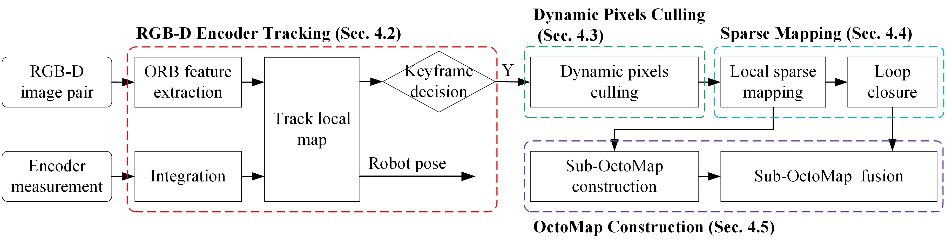
Figure 1 presents a differential-drive robot equipped with an RGB-D camera. Each wheel is mounted with an encoder. We use the following three types of coordinate frames: the world frame $\{w\}$, the camera frame $\{c\}$, and the robot frame $\{r\}$. The world frame $\{w\}$ is coincident with the robot frame $\{r\}$ at the start time. The extrinsic parameters and the kinematics parameters of the robot are precalibrated by [32]. The extrinsic parameters, which are expressed by a $4\times 4$ transformation matrix ${}_c^r\mathbf{T}\in SE\left(3\right)$, are the transformation from the camera frame $\{c\}$ to the robot frame $\{r\}$. The kinematic parameters are the left and right wheel factors $k_l$, $k_r$ and wheel space b. The wheel factors transform the encoder displacement in unit tick to the wheel displacement in unit m. The robot pose is the transformation from the robot frame $\{r\}$ to the world frame $\{w\}$, which is expressed by a $4\times 4$ transformation matrix ${}_r^w\mathbf{T}\in SE\left(3\right)$. In fact, the robot pose only contains three degrees-of-freedom (DoF), as the robot only moves in a 2D plane. Thus, the robot pose can be expressed by a $3\times 1$ vector: ${}_r^w\zeta ={[x,y,\theta ]}^T\in {\mathbb{R}}^3$, ${[x,y]}^T\in {\mathbb{R}}^2$ is the translation, and $\theta \in (-\pi ,\pi ]$ is the yaw angle. Then, ${}_r^w\mathbf{T}$ takes the following form:

$${}_r^w\mathbf{T}=\left[\begin{array}{cccc}cos\left(\theta \right)& -sin\left(\theta \right)& 0& x\\ sin\left(\theta \right)& cos\left(\theta \right)& 0& y\\ 0& 0& 1& 0\\ 0& 0& 0& 1\end{array}\right],$$

(1)

${}_r^w\mathbf{T}$ and ${}_r^w\zeta$ are equivalent. Given ${}_r^w\mathbf{T}$, we can obtain ${}_r^w\zeta$ by the function $F(·)$:

$${}_r^w\zeta =F\left({}_r^w\mathbf{T}\right)=\left[\begin{array}{c}{}_r^w\mathbf{T}\left(1,4\right)\\ {}_r^w\mathbf{T}\left(2,4\right)\\ arctan2\left({}_r^w\mathbf{T}\left(2,1\right),{}_r^w\mathbf{T}\left(1,1\right)\right)\end{array}\right],$$

(2)

where ${}_r^w\mathbf{T}\left(i,j\right)$ is the element in the matrix ${}_r^w\mathbf{T}$ indexed by $\left(i,j\right)$.

The RGB-D camera outputs pairs of color image C and depth image D: $\{C,D\}$. The depth image is preregistered on the color image. We use the pinhole camera model $\pi (·)$, which projects a 3D point ${}^c\mathbf{p}\in {\mathbb{R}}^3$ in the camera frame $\{c\}$ to a 2D point $\mathbf{u}\in {\mathbb{R}}^2$ on the image:

$$\mathbf{u}=\pi \left({}^c\mathbf{p}\right).$$

(3)

The inverse camera model projects a 2D pixel to a 3D point with depth z:

$${}^c\mathbf{p}={\pi }^{-1}\left(\mathbf{u},z\right).$$

(4)

The aim of this paper is to simultaneously estimate the robot pose ${}_r^w\mathbf{T}$ or ${}_r^w\zeta$ and create a static OctoMap in both dynamic and static environments. The map is expressed in the world frame $\{w\}$.

4. Dynamic RGB-D Encoder SLAM (DRE-SLAM)

4.1. System Overview

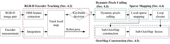
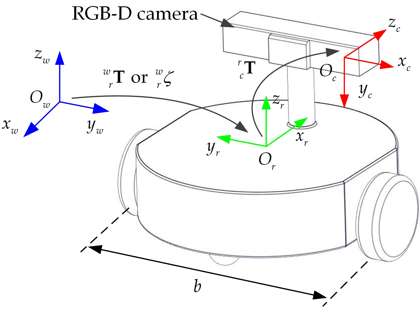
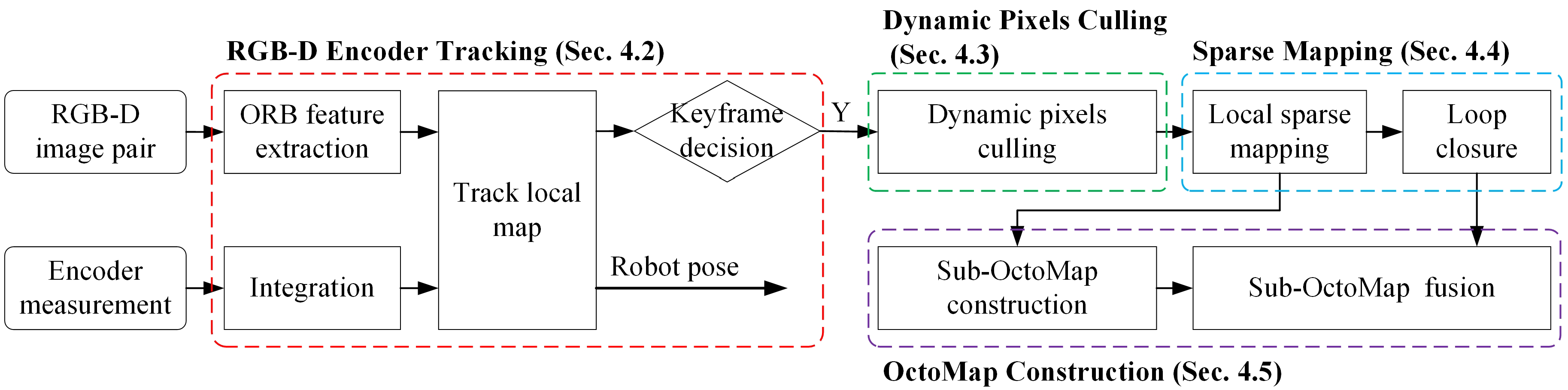
Figure 2 provides an overview of the proposed DRE-SLAM system. This system leverages two types of inputs: the RGB-D image pairs and the encoder measurements. The outputs are a series of robot poses and an OctoMap. The system is based on the sparse feature-based V-SLAM. Coupled with the addition of encoder information and the culling of dynamic pixels, we develop a sparse RGB-D Encoder SLAM for dynamic environments. We then build an OctoMap based on the keyframes. The pipeline is divided into four modules: RGB-D Encoder tracking, dynamic pixels culling, sparse mapping, and OctoMap construction.

RGB-D Encoder Tracking. When an RGB-D pair $\{C,D\}$ comes in, it will be constructed as the current frame and then will be extracted a sparse set of ORB features. As the output frequency of the encoder is generally much higher than that of the camera, we integrate the encoder measurements between the last keyframe and the current frame to obtain a reliable initial robot pose of the current frame to reduce the calculation complexity. The 3D local map points are projected to the current frame to match with the 2D ORB features. The robot pose of the current frame is calculated by jointly minimizing projection errors and encoder errors. Then, whether the current frame is become a new keyframe or not is decided.

Dynamic Pixels Culling. Only the keyframes are used to construct the OctoMap and the sparse map in our system. The key to building a static map in a dynamic environment is identifying and removing the dynamic pixels. This module first detects the predefined dynamic objects in the color image C using an object detection method and then uses multiview constraints to identify dynamic pixels in the depth image D. The dynamic pixels detected by the two approaches are all culled.

Sparse Mapping. Given a new keyframe, this module performs a sliding window local bundle adjustment (BA), which minimizes projection errors and encoder errors. In this way, the robot pose of the new keyframe is refined. The refined new keyframe is sent to the OctoMap construction module. Then, we construct new map points. After this, we detect the loops between the new keyframe and the history keyframes. If a loop is detected, a pose graph optimization will be implemented.

OctoMap Construction. This module uses keyframes to construct sub-OctoMaps first and then assembles these sub-OctoMaps into a full OctoMap. Once the loop closure has completed, we only need to reassemble the sub-OctoMaps.

Our approach runs on six separative threads to obtain real-time operation. The threads are RGB-D encoder tracking, dynamic pixels culling, local sparse mapping, loop closure, sub-OctoMap construction, and sub-OctoMap fusion.

4.2. RGB-D Encoder Tracking

4.2.1. ORB Feature Extraction

We extract 1600 ORB features from the image with resolution of $960\times 540$ pixels produced by a Kinect 2.0 camera. Note that when there are uniform surfaces or fewer textures in the environment, we may not be able to extract enough features in the image. Fortunately, we introduce the encoder information, which enables the system to work properly in these cases. The 2D positions of these features are organized in a KD-Tree to speed up the search process. Homogeneous feature distribution is much more critical for SLAM systems in dynamic scenes because it can reduce the number of feature points on dynamic objects, especially when the dynamic objects contain rich textures. We use the same feature detection policy as the ORB-SLAM2 [1] to obtain a homogeneous feature distribution. The policy divides the image into cells and detects the features in each cell.

4.2.2. Encoder Integration

This section integrates the encoder measurements between the last keyframe and the current frame to obtain the change of the robot pose.

Let the robot pose at time t be ${\zeta }_t={[x_t,y_t,{\theta }_t]}^T$, the robot pose at time $t+1$ is given by the odometry model [33]:

$$\begin{array}{c}\left[\begin{array}{c}{x}_{t+1}\\ y_{t+1}\\ {\theta }_{t+1}\end{array}\right]=\left[\begin{array}{c}{x}_t\\ y_t\\ {\theta }_t\end{array}\right]+\left[\begin{array}{c}\Delta s·cos\left({\theta }_t+0.5\Delta \theta \right)\\ \Delta s·sin\left({\theta }_t+0.5\Delta \theta \right)\\ \Delta \theta \end{array}\right],\hfill \\ \left\{\begin{array}{c}\Delta s=\frac{\Delta s_r+\Delta s_l}{2}\hfill \\ \Delta \theta =\frac{\Delta s_r-\Delta s_l}{b}\hfill \end{array}\right.,\hfill \end{array}$$

(5)

where $\Delta s$ is the translation distance, $\Delta \theta$ is the rotation angle, and $\Delta s_{l/r}$ is the left/right wheel displacement in unit m. $\Delta s_{l/r}$ is given by

$$\left\{\begin{array}{c}\Delta s_r=k_r·\Delta e_r+{\delta }_r,{\delta }_r\sim \mathcal{N}\left(0,{∥K·k_r·\Delta e_r∥}^2\right)\hfill \\ \Delta s_l=k_l·\Delta e_l+{\delta }_l,{\delta }_l\sim \mathcal{N}\left(0,{∥K·k_l·\Delta e_l∥}^2\right)\hfill \end{array}\right.,$$

(6)

where $\Delta e_{l/r}$ is the left/right encoder displacement in unit tick. $\Delta s_{l/r}$ is affected by a zero mean Gaussian noise ${\delta }_{l/r}$, whose standard deviation is proportional to the displacement of the left/right wheel, and the proportionality factor is K. The sources of the noises mainly include the deformation of the wheel, transmission error, encoder error, slight slippage, and so on [33]. The occasional large slippages are not considered in this paper. If a large slippage occurs, the noise model will not be satisfied, which results in large estimation errors. We will solve the slipping problem by the visual information or by adding new sensors in our future work.

Assuming that the robot pose obeys a Gaussian distribution, and the robot pose at time t is ${\zeta }_t\sim \mathcal{N}\left({\overline{\zeta }}_t,{\Sigma }_t\right)$. Then, the covariance of the robot pose at time $t+1$ is given by

$${\Sigma }_{t+1}={\mathbf{G}}^{\zeta }{\Sigma }_t{\left({\mathbf{G}}^{\zeta }\right)}^T+{\mathbf{G}}^s{\Sigma }^s{\left({\mathbf{G}}^s\right)}^T,$$

(7)

where ${\mathbf{G}}^{\zeta }$ is the Jacobian of Equation (5) with respect to the robot pose ${\zeta }_t$, ${\mathbf{G}}^s$ is the Jacobian of Equation (5) with respect to the left and right wheel displacements ${[\Delta s_l,\Delta s_r]}^T$, ${\Sigma }^s$ is the covariance of ${[\Delta s_l,\Delta s_r]}^T$:

$${\Sigma }^s=\left[\begin{array}{cc}{∥K·k_l·\Delta e_l∥}^2& 0\\ 0& {∥K·k_r·\Delta e_r∥}^2\end{array}\right].$$

(8)

Equations (5) and (7) are iteratively used for each encoder measurement between the last keyframe and the current frame. Then, the transformation from the current robot coordinate frame $\{r_c\}$ to the robot coordinate frame $\{r_k\}$ of the last keyframe is obtained: ${}_{r_c}^{r_k}{\mathbf{T}}^e$ or ${}_{r_c}^{r_k}{\zeta }^e\sim \mathcal{N}\left({}_{r_c}^{r_k}{\overline{\zeta }}^e,{}_{r_c}^{r_k}{\Sigma }^e\right)$. We also call it encoder observation in this paper. The superscript symbol e indicates that it is obtained by the encoder measurements.

We only perform encoder integration over a short distance between the current frame with the last keyframe, and between two consecutive keyframes. It ensures the drift of the encoder integration remains within a small range. Furthermore, this drift will be reduced by joint optimization with visual information and by the loop closure.

4.2.3. Local Map Tracking

This section estimates the current robot pose by minimizing the encoder and the projection errors.

The initial robot pose ${}_{r_c}^w{\mathbf{T}}^{\prime }$ of the current frame is propagated from the robot pose ${}_{r_k}^w\mathbf{T}$ of the last keyframe by the encoder integration result:

$${}_{r_c}^w{\mathbf{T}}^{\prime }={}_{r_k}^w\mathbf{T}{}_{r_c}^{r_k}{\mathbf{T}}^e.$$

(9)

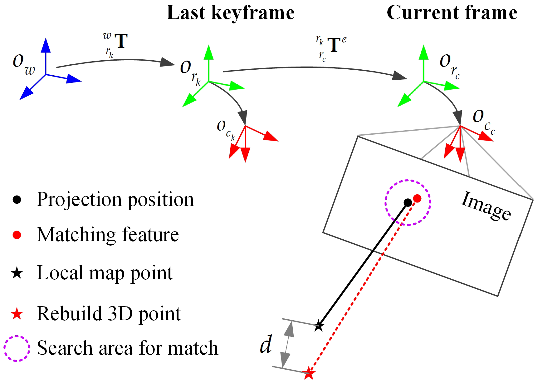
Then, we track the local map. The local map refers to the keyframes (local keyframes) that are close to the current frame in distance and view angle, as well as the map points (local map points) viewed by the local keyframes. The distance threshold $d_{lm}$ is set to 4 m, and the angle threshold ${\theta }_{lm}$ is set to 1 rad in our implementation. The local map points are projected onto the current image to match with the ORB features. Note that the dynamic and static properties of the ORB features of the current frame are unknown, so there may be some erroneous matches. To solve this problem, we propose two policies: (1) limiting the matching search area and (2) using the depth image data to remove erroneous matches. We detail them as follows.

Limiting the matching search area. Thanks to the use of encoder integration, we can search for matching in a small area around the projection position, which improves the matching quality. As shown in Figure 3, a local map point ${}^w\mathbf{p}$ is projected onto the current frame, which results in a 2D position $\mathbf{u}$:

$$\mathbf{u}=\pi \left({\left({}_{r_k}^w\mathbf{T}{}_{r_c}^{r_k}{\mathbf{T}}^e{}_c^r\mathbf{T}\right)}^{-1}{}_{}^w\mathbf{p}\right).$$

(10)

We assume that (1) the local map points are affected by Gaussian noise: ${}^w\mathbf{p}\sim \mathcal{N}\left({}^w\overline{\mathbf{p}},{\Sigma }^p\right)$, (2) the pose of the last keyframe is accurate, and (3) the projection position $\mathbf{u}$ obeys the Gaussian distribution $\mathbf{u}\sim \mathcal{N}\left(\overline{\mathbf{u}},{\Sigma }^u\right)$. Then, the covariance of $\mathbf{u}$ is obtained by

$${\Sigma }^u={\mathbf{G}}^e{}_{r_c}^{r_k}{\Sigma }^e{\left({\mathbf{G}}^e\right)}^T+{\mathbf{G}}^p{\Sigma }^p{\left({\mathbf{G}}^p\right)}^T,$$

(11)

where ${\mathbf{G}}^e$ is the Jacobian of Equation (10) with respect to the encoder observation ${}_{r_c}^{r_k}{\mathbf{T}}^e$ or ${}_{r_c}^{r_k}{\zeta }^e$, ${\mathbf{G}}^p$ is the Jacobian of Equation (10) with respect to the local map point position ${}^w\mathbf{p}$. Then, we can search for matching within the $3\sigma$ boundary around the projection position $\mathbf{u}$. However, the $3\sigma$ boundary is typically an ellipse, which is difficult to search in. To speed up the matching, we use the radius search method of KD-Tree by using the envelope circle of the $3\sigma$ ellipse as the matching search area. Thus, a matching ORB feature is obtained by searching the best match in this area.

Using the depth image data to remove erroneous matches. As shown in Figure 3, if an effective depth value $z^{\prime }$ can be found on the position ${\mathbf{u}}^{\prime }$ of the matching feature in the depth image, we can rebuild a 3D map point:

$${}^w{\mathbf{p}}^{\prime }={}_{r_k}^w\mathbf{T}{}_{r_c}^{r_k}{\mathbf{T}}^e{}_c^r\mathbf{T}{\pi }^{-1}\left({\mathbf{u}}^{\prime },z^{\prime }\right).$$

(12)

If the matching feature and the map point are both static and the match is correct, the difference between ${}^w\mathbf{p}$ and ${}^w{\mathbf{p}}^{\prime }$ is generally small. However, if there are dynamic feature or map point in the match or the match is incorrect, the difference tends to be large. We use the distance d between ${}^w\mathbf{p}$ and ${}^w{\mathbf{p}}^{\prime }$ to measure the difference. Then, we can use a threshold $d_{th}$ to determine the correct match and the erroneous match. The distance d is influenced by the error of the robot pose, the map point, and the depth image for the correct matches. The assumption of using the depth image to filter out erroneous matches is that the accuracy of the RGB-D sensor must be high enough. If the depth error is too large, the distance d of a correct match will be large, and the correct match may be mistakenly considered to be an erroneous match. The Kinect 2.0 camera used in this paper has sufficient accuracy to remove the erroneous matches. We set the threshold $d_{th}$ to grow linearly with the depth value $z^{\prime }$, as the depth error of RGB-D camera increases with distance.

$$d_{th}=d_b+k_d·z^{\prime }.$$

(13)

where $d_b$ is the base threshold and $k_d$ is the scale factor. We set $d_b=0.2$ m and $k_d=0.025$ in this paper.

Given the encoder observation between the last keyframe and the current frame (see Section 4.2.2), as well as the 3D–2D matches, the pose of the current frame is refined by minimizing the encoder error and the projection errors:

$${}_{r_c}^w{\mathbf{T}}^{*}=\underset{{}_{r_c}^w\mathbf{T}}{argmin}\left(E_{enc}+\sum _{i\in \mathcal{R}}{E}_{i,proj}\right),$$

(14)

where $\mathcal{R}$ contains all 3D–2D matches. The encode error is defined by

$$E_{enc}=\rho \left({\left({\mathbf{e}}^e\right)}^T{\left({}_{r_c}^{r_k}{\Sigma }^e\right)}^{-1}{\mathbf{e}}^e\right),{\mathbf{e}}^e={}_{r_c}^{r_k}{\zeta }^e-F\left({\left({}_{r_k}^w\mathbf{T}\right)}^{-1}{}_{r_c}^w\mathbf{T}\right),$$

(15)

where $\rho \left(·\right)$ is the Huber robust cost function. $F\left(·\right)$ converts a $4\times 4$ homogenous transformation matrix to a $3\times 1$ vector. The projection error for each 3D–2D match is defined by

$$E_{i,proj}=\rho \left({\left({\mathbf{e}}_i^v\right)}^T{\left({\Sigma }_i^v\right)}^{-1}{\mathbf{e}}_i^v\right),{\mathbf{e}}_i^v={{\mathbf{u}}^{\prime }}_i-\pi \left({\left({}_{r_c}^w\mathbf{T}{}_c^r\mathbf{T}\right)}^{-1}{}^w{\mathbf{p}}_i\right),$$

(16)

where $\rho \left(·\right)$ is the Huber robust cost function, and ${\Sigma }_i^v$ is the feature covariance, which is associated with the ORB feature scale.

4.2.4. Keyframe Decision

The current frame will be constructed as a new keyframe if the following conditions are all satisfied.

• $N_{pf}$ frames have passed from the last keyframe. This condition guarantees enough time between two adjacent keyframes allow for the dynamic pixels culling, sparse mapping, and OctoMap construction. We set $N_{pf}$ to be the output frequency of the RGB-D camera to ensure at least 1 s of time is between the two adjacent keyframes. If the robot moves too fast, the distance between two consecutive keyframes may be too large, which results in too much encoder integration error. The two erroneous match detection policies in Section 4.2.3 may be invalid. The system accuracy is reduced. Then, there will be no enough co-view part for the mapping. Thus, we recommend operating the robot at a slow speed, e.g., lower than 0.4 m/s.
• The distance or angle between the current frame and the last keyframe is larger than threshold $d_{kf}$ or ${\theta }_{kf}$, respectively. On the one hand, this ensures that the encoder integration does not diverge too much, thus ensuring the functional of erroneous match detection and the accuracy of robot pose tracking. On the other hand, it ensures enough viewing overlaps between keyframes for OctoMap construction. In our implementation, we set these two parameters as $d_{kf}=0.3$ m and ${\theta }_{kf}=0.5$ rad.

4.3. Dynamic Pixels Culling

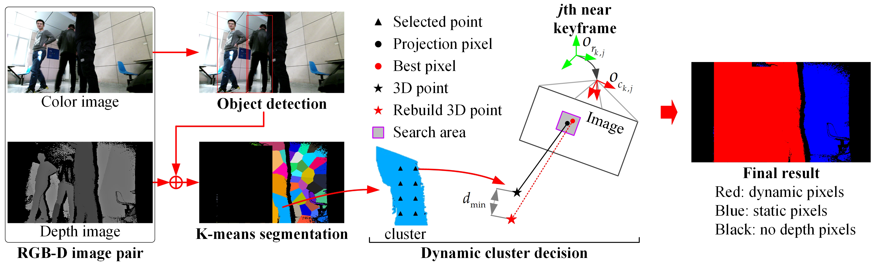
Figure 4 shows the dynamic pixels culling pipeline. The object detection and multiview geometry constraints are combined to detect dynamic pixels in the new keyframe.

4.3.1. Objects Detection

We detect predefined dynamic objects from the color image. In an indoor environment, dynamic objects may be person, cat, dog, etc. We detect these predefined dynamic objects by the object detection method YOLOv3 [34] that is implanted in OpenCV. The publicly available model trained on the COCO dataset [35] is directly used. The YOLOv3 can process 6–7 images per second on our Intel i7-8700 CPU, without the need of a GPU. However, there may be some miss-detections, especially when only a part of a dynamic object is viewed, as shown in Figure 4. Furthermore, some objects that are not included in the predefined dynamic objects may also be moving, such as books, chairs, and desks. Thus, a method based on a multiview constraint is proposed to detect dynamic pixels using the depth image in the following.

4.3.2. Multiview Constraint-Based Dynamic Pixels Culling

As shown in Figure 4, the pixels in bounding boxes of dynamic objects are culled first. Then, the remanding pixels are projected to 3D to create a point cloud. We use the K-means method to segment the point cloud into several clusters. The clusters are assumed to be rigid bodies, which means that the pixels in the same cluster have the same motion property. This assumption is reasonable because we focus on removing dynamic pixels and building static maps but not tracking dynamic objects. The number of clusters, k, is determined according to the size $s_p$ of the point cloud: $k=s_p/n_{pt}$. $n_{pt}$ is the average point number of a cluster to be adjusted. Reducing $n_{pt}$ guarantees a better approximation, but it also increases the computational burden. We set $n_{pt}$ to be 6000 to balance the computational consumption and precision.

We only need to detect which clusters are dynamic ones. To speed up the dynamic cluster detection process, we only select a small number of pixels (e.g., 100) uniformly in a cluster and then use the multiview constraint to judge their dynamic and static attributes. If the number of dynamic pixels is large, the cluster is determined to be dynamic. Otherwise, the cluster is determined to be static.

We detect whether a pixel is dynamic by projecting it to the last $N_{pc}$ keyframes (near keyframes) for comparison. We set $N_{pc}=5$ in this paper. The pixels $\mathbf{u}$ are back projected to be a 3D point in the world frame using its depth z in the depth image and the robot pose ${}_{r_{kn}}^w\mathbf{T}$ of the new keyframe:

$${}^w\mathbf{p}={}_{r_{kn}}^w\mathbf{T}{}_c^r\mathbf{T}{\pi }^{-1}\left(\mathbf{u},z\right).$$

(17)

The 3D point ${}^w\mathbf{p}$ can be projected onto the image of the jth near keyframe:

$${\mathbf{u}}^{\prime }=\pi \left({\left({}_{r_{k,j}}^w\mathbf{T}{}_c^r\mathbf{T}\right)}^{-1}{}^w\mathbf{p}\right),$$

(18)

where ${}_{r_{k,j}}^w\mathbf{T}$ is the robot pose of the jth near keyframe. If the pixel ${\mathbf{u}}^{\prime }$ of the depth image of the jth keyframe has a valid depth $z^{\prime }$, a rebuilt 3D point ${}^w{\mathbf{p}}^{\prime }$ can be obtained as

$${}^w{\mathbf{p}}^{\prime }={}_{r_{k,j}}^w\mathbf{T}{}_c^r\mathbf{T}{\pi }^{-1}\left({\mathbf{u}}^{\prime },z^{\prime }\right).$$

(19)

Note that the dynamic pixels of the depth image of the jth keyframe have been culled before. If a pixel is static, the distance d between ${}^w{\mathbf{p}}^{\prime }$ and ${}^w\mathbf{p}$ should be very small. Otherwise, this pixel is a dynamic pixel. Considering that both the depth image and the poses of the keyframes have errors, ${\mathbf{u}}^{\prime }$ may not be the pixel corresponding to $\mathbf{u}$, so we search for a pixel within a square around ${\mathbf{u}}^{\prime }$ so that d takes the minimum value $d_{min}$. The square size $s_z$ is affected by the keyframe accuracy and depth image accuracy. We empirically set the square size $s_z$ to 9 pixels. If $d_{min}$ is larger than a threshold $d_{mth}$, the pixel ${\mathbf{u}}^{\prime }$ is judged as a dynamic pixel in this projection step, otherwise it is a static pixel. The threshold $d_{mth}$ is determined by the keyframe accuracy and depth image accuracy. Same as Equation (10), we also set the threshold $d_{mth}$ to grow linearly with the depth value $z^{\prime }$. The other situations are that no valid depth values can be found in the square search area or ${\mathbf{u}}^{\prime }$ is out of the range of the image. In this situation, the pixel $\mathbf{u}$ is judged as invalid. We can judge whether a pixel $\mathbf{u}$ is dynamic, static, or invalid by projecting it to one keyframe now. Given that the result of one keyframe is not reliable enough and may produce invalid results, we apply the above process to all near keyframes. Finally, the property of a pixel is determined by voting. Assuming the number of static results is $N_s$, the number of dynamic results is $N_d$, and the number of invalid results is $N_i$, the final decision of the pixel $\mathbf{u}$ is given by

$$\left\{\begin{array}{c}static,if(N_s\ge N_d,N_s>0)\hfill \\ dynamic,if(N_d>N_s,N_d>0)\hfill \\ invalid,if(N_s=N_d=0)\hfill \end{array}\right..$$

(20)

Similarly, we also use the voting approach to determine the properties of a cluster. Among the selected pixels in one cluster, assuming that the number of static ones are $N_s^{\prime }$, the number of dynamic ones are $N_d^{\prime }$, and the number of invalid ones are $N_i^{\prime }$, the final property of the cluster is

$$\left\{\begin{array}{c}static,if({N^{\prime }}_s\ge {N^{\prime }}_d)\hfill \\ dynamic,if({N^{\prime }}_d>{N^{\prime }}_s)\hfill \end{array}\right..$$

(21)

The final static pixels are obtained by culling the pixels in the dynamic clusters and in the bounding boxes of the potential dynamic objects, as shown in Figure 4. It should be noted that some static pixels in the bounding box are also removed as dynamic pixels. This is acceptable because we focus on eliminating dynamic interference and dynamic data in the OctoMap. The remaining static pixels can satisfy the needs of the OctoMap construction.

4.4. Sparse Mapping

4.4.1. Sparse Mapping

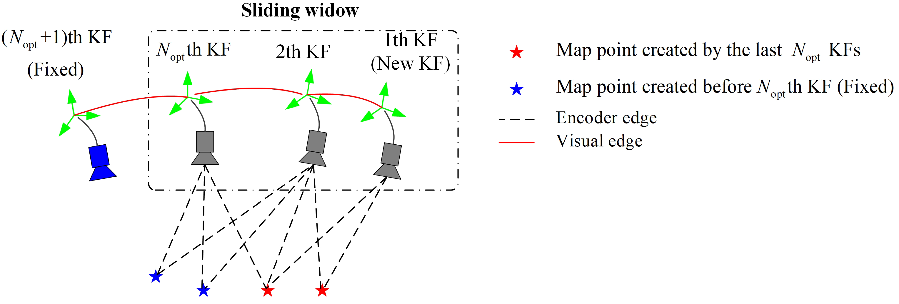
A sliding window local bundle adjustment is applied as shown in Figure 5. The states participating in the optimization are the robot poses of the last $N_{opt}$ keyframes, the last $\left(N_{opt}+1\right)$th keyframe, as well as the map points not only observed by the last $N_{opt}$ keyframes but also observed by at least two keyframes. The last $\left(N_{opt}+1\right)$th keyframe and the map points created before the $N_{opt}$th keyframe are fixed during the optimization. The cost function is defined by

$$\underset{}{argmin}\left(\sum _{l=1}^{N_{opt}}{E}_{enc}\left(l,l+1\right)+\sum _{\left(i,l\right)\in \chi }{E}_{proj}\left(i,l\right)\right).$$

(22)

$E_{enc}\left(l,l+1\right)$ defines the encoder error between the lth and the $(l+1)$th keyframe. It is the same as Equation (15). $E_{proj}(i,l)$ is the projection error term of the ith map point to the last lth keyframe. It is the same as Equation (16). $\chi$ contains all projection pairs. We set the sliding window size $N_{opt}$ to 8 KFs to balance the computing time and the accuracy.

After local optimization, the robot pose of the new static keyframe is refined. It is then sent to the OctoMap construction module. After that, new map points are created. As dynamic pixels have been discarded, the map points created are all static map points.

4.4.2. Loop Closure

The loop detection is carried out for every new keyframe using the bag-of-words approach DBow2 [36]. Once a loop is detected, the pose graph optimization will be performed. Since the map points are all static, the loop closure avoids interferences from moving objects. All the abovementioned optimizations are performed by the Ceres Solver [37].

4.5. OctoMap Construction

OctoMap divides the 3D space into voxels and stores these voxels through the octree structure, which effectively reduces the memory cost. Each voxel is given an occupancy probability. This probability is updated by integrating multiple observations $z_{1:t}$ through a binary Bayesian filter [14]:

$$P\left(o|z_{1:t}\right)=\left[1+\frac{1-P\left(o|z_t\right)}{P\left(o|z_t\right)}\frac{1-P\left(o|z_{1:t-1}\right)}{P\left(o|z_{1:t-1}\right)}\frac{P\left(o\right)}{1-P\left(o\right)}\right],$$

(23)

where $P\left(o\right)$ is the prior, which is often set to 0.5. By using log-odds notation, Equation (23) can be rewritten as

$$L\left(o|z_{1:t}\right)=L\left(o|z_{1:t-1}\right)+L\left(o|z_t\right),L\left(o\right)=log\left(\frac{P\left(o\right)}{1-P\left(o\right)}\right).$$

(24)

The measurement integration into a voxel becomes a simple log-odds addition. Typically, a clamping update policy that defines the upper and lower bound on the occupancy probability is applied:

$$L\left(o|z_{1:t}\right)=max(min(L\left(o|z_{1:t}\right),l_{max}),l_{min}),$$

(25)

where $l_{max}$ and $l_{min}$ are the upper and lower log-odds bounds. The clamping update policy ensures the confidence in the map remains bounded. As a consequence, the model can adapt to environment changes quickly [14].

OctoMap is suitable for robot navigation. However, it is not deformable. When a loop is detected and the poses of the keyframes are adjusted, the full OctoMap should be rebuild by retracing all the raw data. To tackle this problem, as shown in Figure 6, this section first creates a series of sub-OctoMaps, then fuses them to form a full OctoMap. The sub-OctoMap integrates raw measurements to a small OctoMap, which saves memory space compared with storing raw data. We just need to refuse the sub-OctoMaps after the loop closure, which speeds up the rebuilding process.

4.5.1. Sub-OctoMap Construction

Generally, within the consecutive $N_{sub}$ keyframes, the robot pose error is bounded within a small range. Therefore, we construct the $N_{sub}$ keyframes as a local sub-OctoMap $S_i$. We call $N_{sub}$ the submap size. The sub-OctoMap is built relative to a local coordinate frame that is set to be the robot coordinate frame of the first keyframe in this sub-OctoMap. We denote its pose relative to the world coordinate frame as ${}_{S_i}^w\mathbf{T}$. The measurements of the depth images in these keyframes are integrated into the sub-OctoMap by performing a ray castings operation from the RGB-D camera to the end points.

4.5.2. Sub-OctoMap Fusion

This section fuses all sub-OctoMaps $\left\{\left\{S_1,{}_{S_1}^w\mathbf{T}\right\},\left\{S_2,{}_{S_2}^w\mathbf{T}\right\},\cdots \left\{S_n,{}_{S_n}^w\mathbf{T}\right\}\right\}$ to form a full OctoMap. The full OctoMap is constructed in reference to the world frame $\{w\}$. The process is to transform all sub-OctoMap voxels into the full OctoMap and fuse the occupancy probabilities. For one submap $\left\{S_i,{}_{S_i}^w\mathbf{T}\right\}$, the center position of one voxel $V_{S_i}$ in its local frame is ${}^{S_i}\mathbf{p}$, and we transform it to the world frame:

$${}^w\mathbf{p}={}_{S_i}^w\mathbf{T}{}^{S_i}\mathbf{p}.$$

(26)

Assuming ${}^w\mathbf{p}$ falls into the voxel $V_{F_j}$ of the full OctoMap, the log-odds of $V_{S_i}$ is $L_{S_i}$, and the log-odds $L_{F_j}$ of voxel $V_{F_j}$ is then updated by simple addition:

$$L_{F_j}=L_{F_j}+L_{S_i}.$$

(27)

The clamping update policy is also used. In this way, we transform the voxels of all sub-OctoMaps into the world coordinate frame to fuse the sub-OctoMaps. Once the pose graph has been adjusted, we just need to refuse these sub-OctoMaps.

This section has two parameters to be turned. One is the voxel size of the OctoMap. The smaller the voxel is, the larger the memory and the amount of computation required. The other is the size of the submap; a submap that is too large will cause distortion of the full map. The impact of these two parameters on the time and memory costs will be explored in the experiment (see Section 5.4).

It should be noted that this submap-based method reduces the precision of the full OctoMap, because the precision of the point cloud is compressed to the voxel size when building the sub-OctoMaps. Furthermore, we use the center point of a voxel as its position when fusing the sub-OctoMaps.

4.6. System Initialization

The system is initialized by constructing the first RGB-D image pair as the first keyframe. The dynamic pixels are culling only by objects detection, as no other keyframes are available. After the dynamic pixels have been culled, we create a number of map points.

5. Experiments

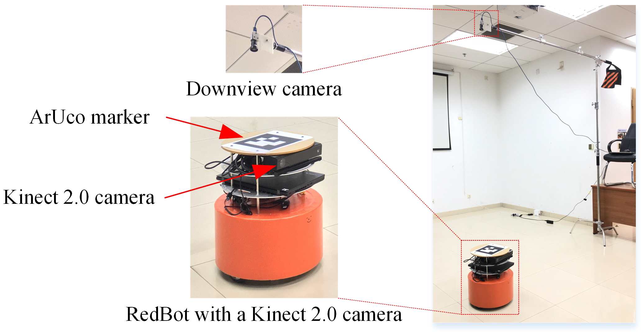
This section evaluates the proposed DRE-SLAM system by self-collected data in various dynamic and static environments. The data were collected by the RedBot using Rosbag tools [38], as shown in Figure 7. Each wheel of RedBot has been mounted an encoder that outputs measurements in a frequency of 100 Hz. A Kinect 2.0 camera is fixed at the front of the robot. The camera outputs registered RGB-D image pairs at a rate of 20 Hz with a resolution of $960\times 540$ pixels by using the iai-kinect2 driver [39]. We implemented the proposed DRE-SLAM in C++ and performed all experiments on a computer with Intel Core i7-8700 CPU, 16 GB RAM. The operating system is Ubuntu 16.04.

5.1. Comparative Tests

This section compares the proposed DRE-SLAM with three other state-of-the-art open source SLAM systems in terms of pose accuracy, map quality, and robustness. The chosen systems are: RTAB-MAP [15], StaticFusion [17], and Co-Fusion [7]. The StaticFusion and Co-Fusion were performed on a GTX1070 GPU. Since some scenes are not close to the camera in our experiments, we used depth pixels within a distance 8.0 m of the depth map for all of the four methods. The other special configurations are as follows:

DRE-SLAM. In the OctoMap construction module, the voxel size of the OctoMap was set to 0.05 m, the submap size was set to five keyframes.

RTAB-MAP. This system takes RGB-D images and the wheel odometry as inputs. We integrated the wheel-encoder measurements to form the wheel odometry for the RTAB-MAP. Its OctoMap voxel size was also set to 0.05 m. All other parameters were set to original.

StaticFusion. This system only uses RGB-D images and outputs a static surfel-based background map. The original implementation is for images of $640\times 480$ pixels that are downsampled to $320\times 240$ pixels in the program. We modified the interface to accept images of $960\times 540$ pixels, and we also downsampled the images to $480\times 270$ pixels in the program. The other parameters were not changed.

Co-Fusion. This system constructs a surfel-based background map and tracks moving objects only using RGB-D image pairs. As we only consider the background construction, we deactivated its tracking part.

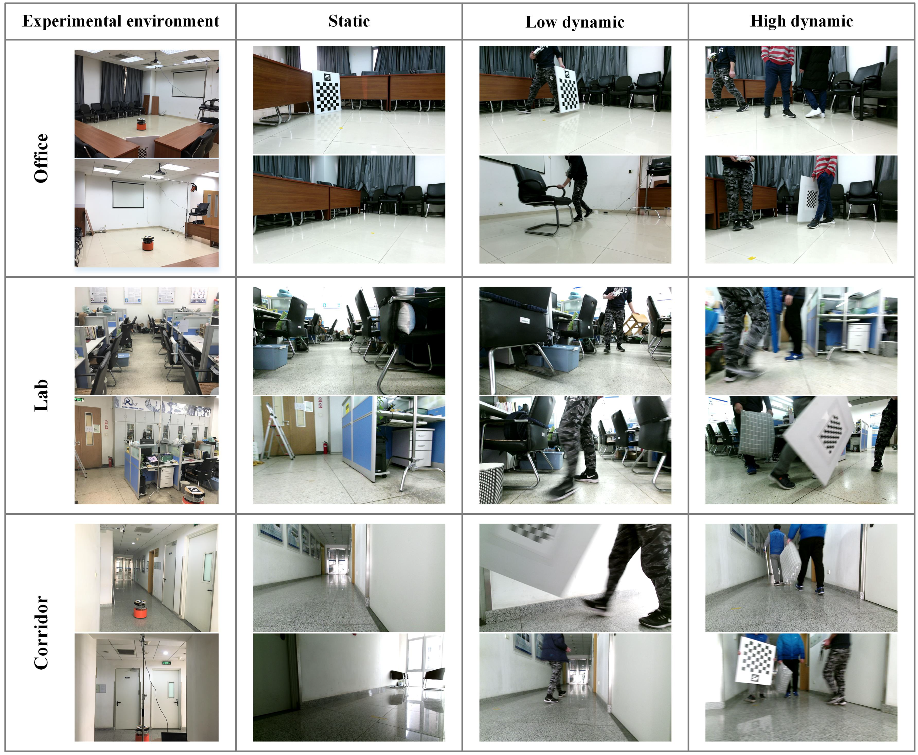
As shown in Figure 8, we collected data in three different environments: office (O), laboratory (L), and corridor (C). The office environment is clean and tidy. The lab environment is messy and rich in texture and structure information. The corridor environment is full of white walls and less in texture and structure information. We collected three types of data, static (ST), low dynamic (LD), and high dynamic (HD), in each environment. In the static data, there are no moving objects. In the low dynamic data, only one person is moving. In the high dynamic data, three persons are moving. The persons move with tablets, chairs or other undefined objects. The purpose is to verify the recognition capability of the dynamic pixels on undefined objects. Three sequences were collected for each type of data. A total of 27 sequences were collected for the comparative tests. Each data sequence is named using the environment type and data type. For example, O-ST1 is the first sequence collected in the static (ST) office (O) environment. The four approaches were tested in all these 27 sequences.

5.1.1. Pose Accuracy

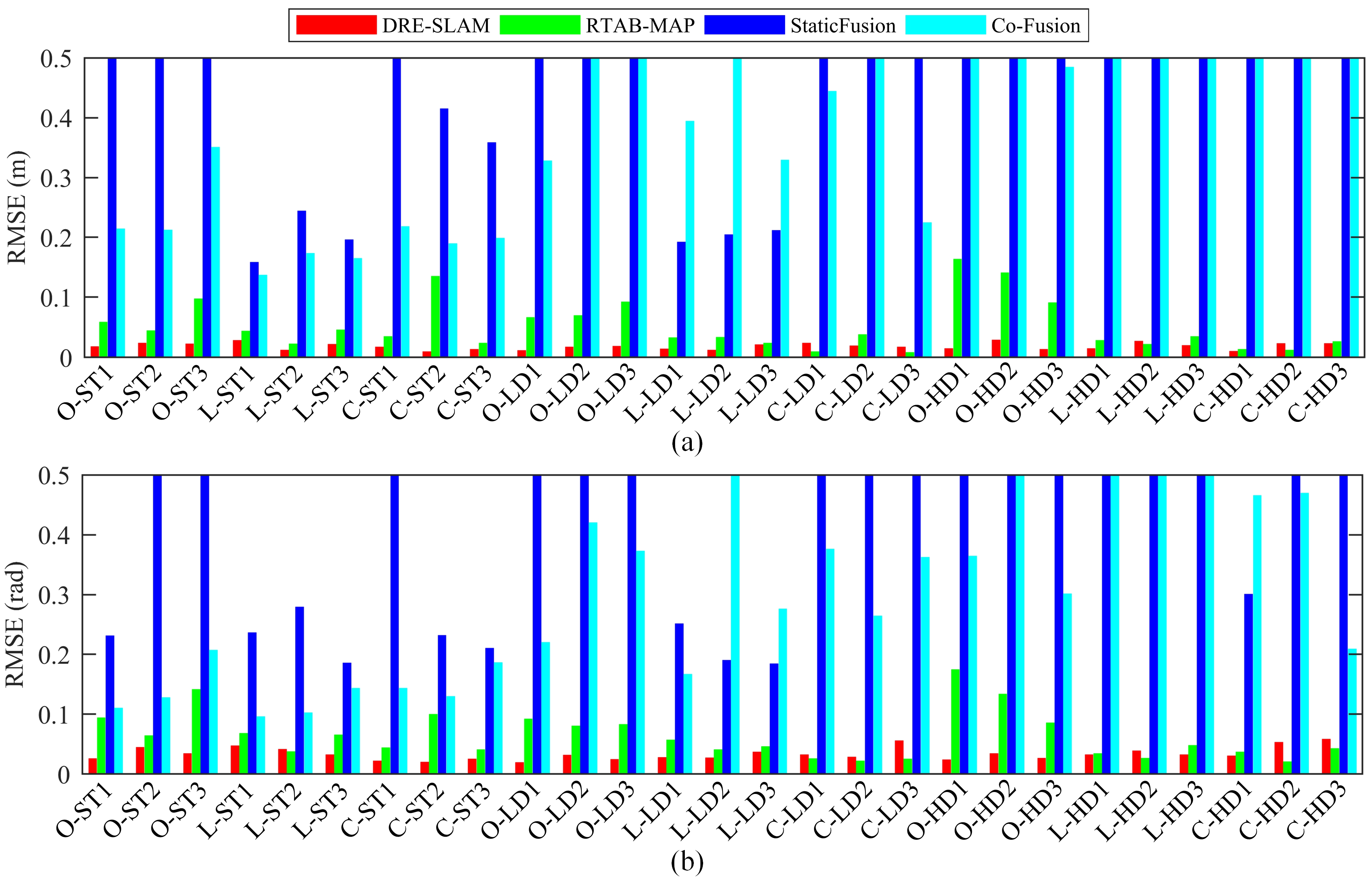
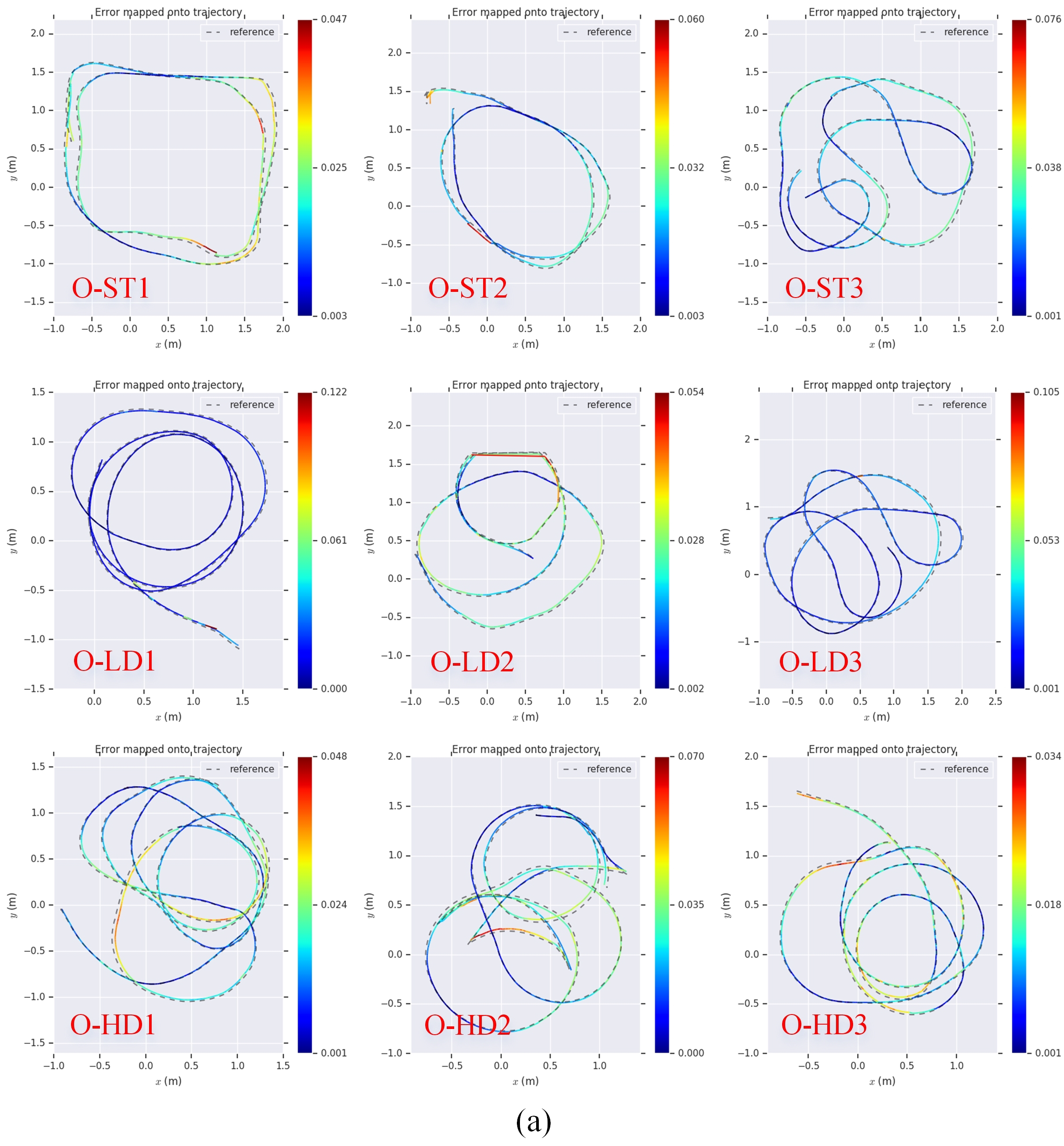
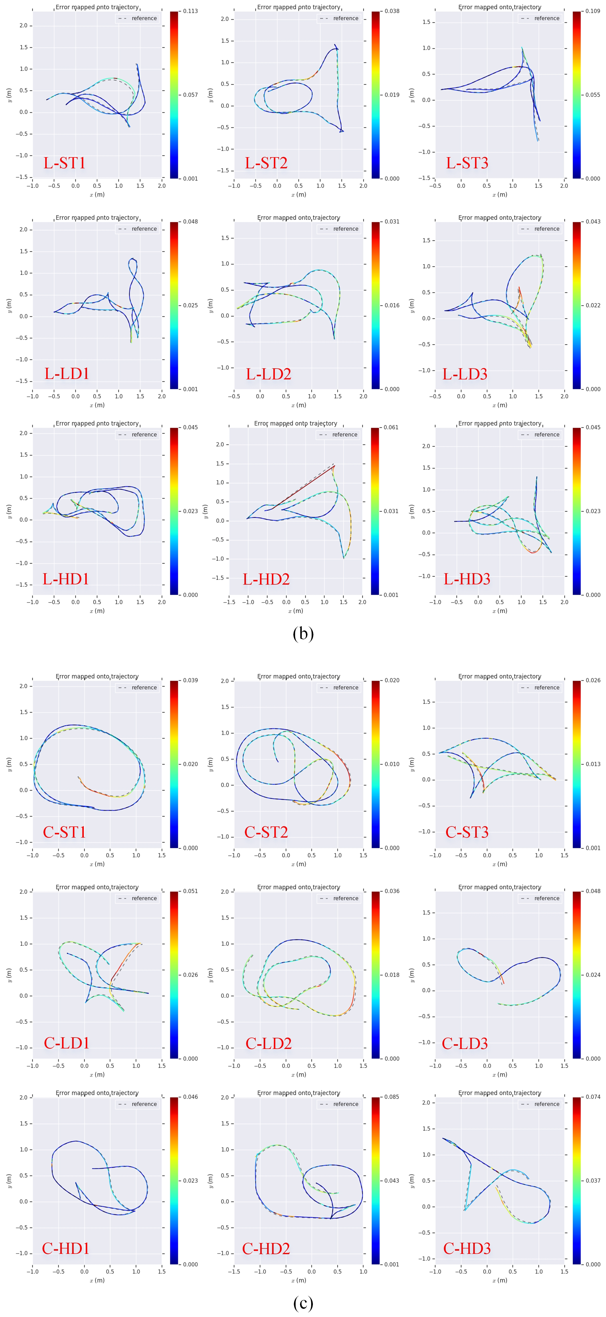
As shown in Figure 7, we mounted an ArUco [40] marker on the top of the RedBot and used a fixed downview camera to capture the marker to produce the pose ground truth by using a plane measurement method [41]. The absolute pose error (APE) metric is used to evaluate the pose accuracy with the evo tool [42]. The results are shown in

Table 1. The root-mean-square-error (RMSE) of the translation (m) and the rotation (rad) of the four methods in all the sequences. The numbers in bold represent the minimum results.

Sequences	DRE-SLAM		RTAB-MAP		StaticFusion		Co-Fusion
	Trans.	Rot.	Trans.	Rot.	Trans.	Rot.	Trans.	Rot.
O-ST1	0.0171	0.0252	0.0574	0.0934	0.6896	0.2304	0.2136	0.1091
O-ST2	0.0233	0.0436	0.0429	0.0633	2.2755	2.8240	0.2114	0.1266
O-ST3	0.0218	0.0335	0.0964	0.1406	3.4684	1.8022	0.3499	0.2061
L-ST1	0.0274	0.0461	0.0422	0.0672	0.1575	0.2352	0.1361	0.0950
L-ST2	0.0116	0.0403	0.0216	0.0364	0.2429	0.2784	0.1726	0.1017
L-ST3	0.0212	0.0315	0.0447	0.0648	0.1951	0.1846	0.1641	0.1427
C-ST1	0.0162	0.0209	0.0339	0.0433	0.8425	0.6428	0.2174	0.1427
C-ST2	0.0088	0.0192	0.1342	0.0991	0.4140	0.2310	0.1889	0.1287
C-ST3	0.0129	0.0246	0.0228	0.0401	0.3572	0.2095	0.1980	0.1852
O-LD1	0.0108	0.0185	0.0655	0.0915	1.0082	1.1706	0.3272	0.2191
O-LD2	0.0162	0.0309	0.0683	0.0797	0.7561	0.8079	0.7212	0.4193
O-LD3	0.0175	0.0236	0.0915	0.0818	2.0426	2.6095	1.2238	0.3720
L-LD1	0.0133	0.0270	0.0321	0.0561	0.1912	0.2503	0.3934	0.1662
L-LD2	0.0110	0.0262	0.0325	0.0396	0.2037	0.1894	0.5229	0.6387
L-LD3	0.0206	0.0358	0.0227	0.0451	0.2105	0.1836	0.3281	0.2751
C-LD1	0.0231	0.0317	0.0087	0.0252	1.4949	1.2988	0.4433	0.3749
C-LD2	0.0184	0.0274	0.0374	0.0211	2.4187	1.4065	0.6043	0.2630
C-LD3	0.0164	0.0549	0.0072	0.0246	3.2005	2.5659	0.2238	0.3615
O-HD1	0.0141	0.0229	0.1627	0.1739	4.7680	2.4754	0.7468	0.3635
O-HD2	0.0284	0.0331	0.1396	0.1329	2.2350	2.6707	0.7736	1.0450
O-HD3	0.0127	0.0256	0.0896	0.0846	0.8233	1.3533	0.4835	0.3002
L-HD1	0.0136	0.0317	0.0277	0.0332	2.6896	1.2771	1.2393	1.1438
L-HD2	0.0262	0.0380	0.0211	0.0258	1.4187	2.0547	0.8072	1.0425
L-HD3	0.0190	0.0314	0.0340	0.0471	2.1998	2.1153	0.7263	0.6762
C-HD1	0.0095	0.0292	0.0127	0.0357	0.5868	0.2994	0.8212	0.4649
C-HD2	0.0225	0.0519	0.0111	0.0195	1.8197	2.8022	1.3695	0.4685
C-HD3	0.0222	0.0575	0.0257	0.0416	1.3683	2.3261	0.5095	0.2080

. The root-mean-square-error (RMSE) comparison is shown in Figure 9. It can be seen that DRE-SLAM obtains the highest accuracy in most sequences against the other three methods. Moreover, the pose errors are not much different, whether in static environments or in dynamic environments. This shows that DRE-SLAM is rarely affected by dynamic objects in terms of pose accuracy. The pose errors of RTAB-MAP in most sequences are also relatively small. However, the pose errors increase in dynamic sequences in the office environment, especially in high dynamic sequences. This is because RTAB-MAP does not consider dynamic interference in the loop and proximity detection, whereas DRE-SLAM eliminates dynamic pixels and is, therefore, unaffected by dynamic objects. Furthermore, RTAB-MAP only uses the wheel odometry for the current robot pose estimation, whereas DRE-SLAM tightly couples the information of the RGB-D camera with the wheel-encoders. StaticFusion possesses large pose errors in most sequences. Co-Fusion performs small errors most static environments, whereas the errors increase dramatically in dynamic environments. The reasons for the large errors in StaticFusion and Co-Fusion may be that (1) the scene is too far away or (2) there is no encoder data. This also shows that using the encoder improves the system accuracy, especially in dynamic environments. The use of the encoder information can provide good prior and strong constraints. When the static pixel is missing, the encoder can also obtain a reliable pose estimation. We also provide the trajectories of DRE-SLAM with the ground truths in Figure 10. The trajectories of DRE-SLAM are smooth and fit well with the ground truth.

5.1.2. Map Quality

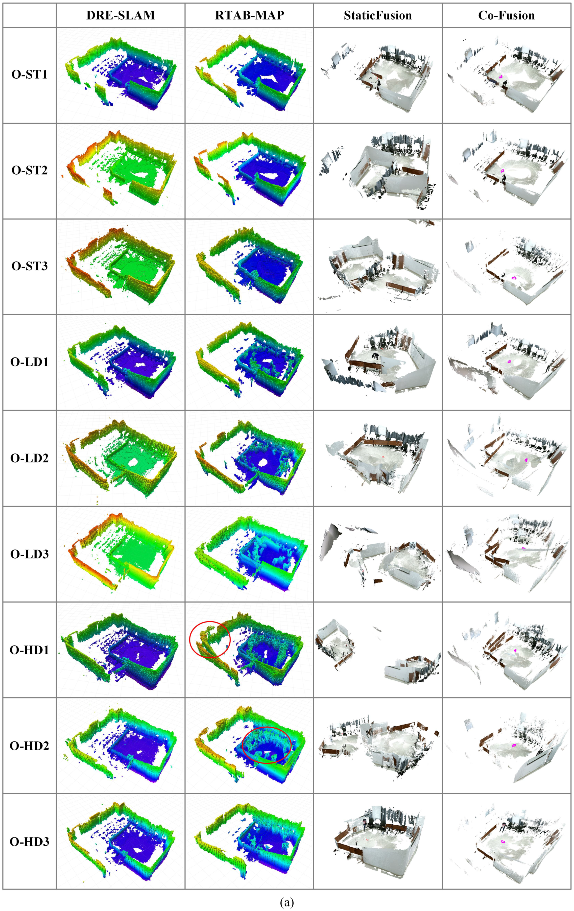
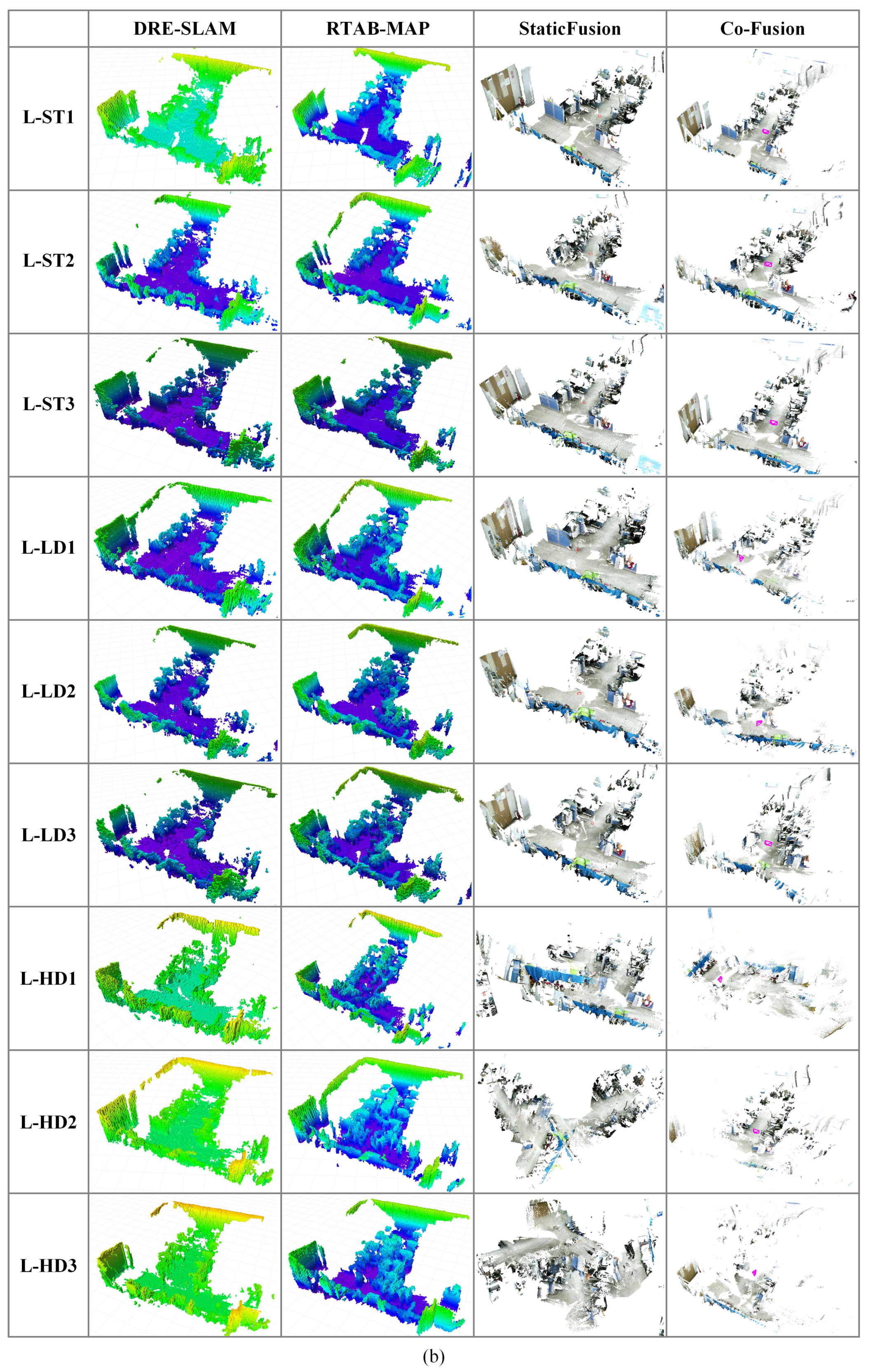
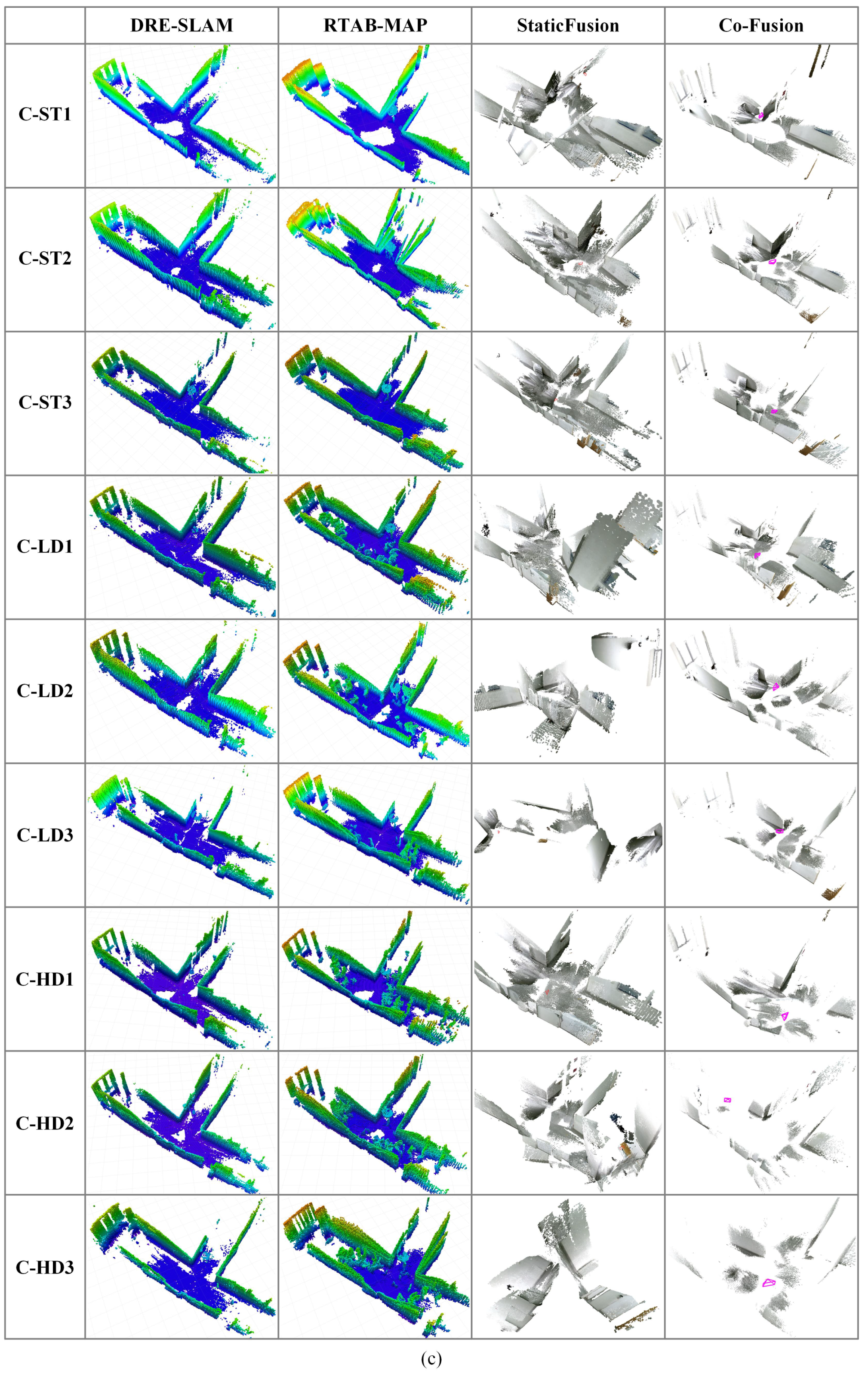
Figure 11 provides all maps created by the four methods with all the data sequences. DRE-SLAM constructed clean background maps in most sequences. There are no obvious distortions in these maps. This proves that DRE-SLAM can reliably construct static maps in both dynamic and static environments. The RTAB-MAP constructs nice maps in most static sequences. However, many dynamic objects are introduced in its maps in the low and high dynamic sequences. Some maps even contain obvious distortions, e.g., maps of O-HD1and C-ST2. StaticFusion obtains nice maps in the static and low dynamic lab sequences. This may benefit from the rich structure of the lab environment. However, in other sequences, its maps suffer a lot of distortions. We find that StaticFusion treats many static pixels as dynamic pixels. Co-Fusion can build correct maps in most static sequences, but the maps are obviously confusing in the low and high dynamic sequences. We can also see that DRE-SLAM and RTAB-MAP, which fuse encoder information, produce maps with fewer distortions. Whereas the pure RGB-D methods, StaticFusion and Co-Fusion, create maps with more distortions. This phenomenon indicates that using the encoder is helpful to improve the map quality. The quality of the map is mainly determined by the pose accuracy of the keyframes and the dynamic pixels’ culling effect. The sounder map quality of our system in Figure 11 further shows that our method produces high pose accuracy and a dynamic pixel culling effect.

5.1.3. Robustness

DRE-SLAM achieves accurate pose estimation and impressive static maps in all sequences, even when there are dynamic objects in the environments. This shows the robustness of the system. RTAB-MAP also works reliably on most sequences because its local pose estimation only relies on wheel odometry. Only the loop closure and proximity detection use visual information that is confused by dynamic objects. However, the pure RGB-D methods, StaticFusion and Co-Fusion, are fragile. They cannot work reliably even in a static environment. This is because it is difficult to achieve reliable estimation if the number of identified static pixels is too small, which leads to the whole system collapse. However, if the encoder information is added, the encoder can work reliably over a short distance even if the visual information is completely lost. In short, combining of the RGB-D camera and encoders creates a highly robust system.

5.2. Performance of Dynamic Pixels Culling

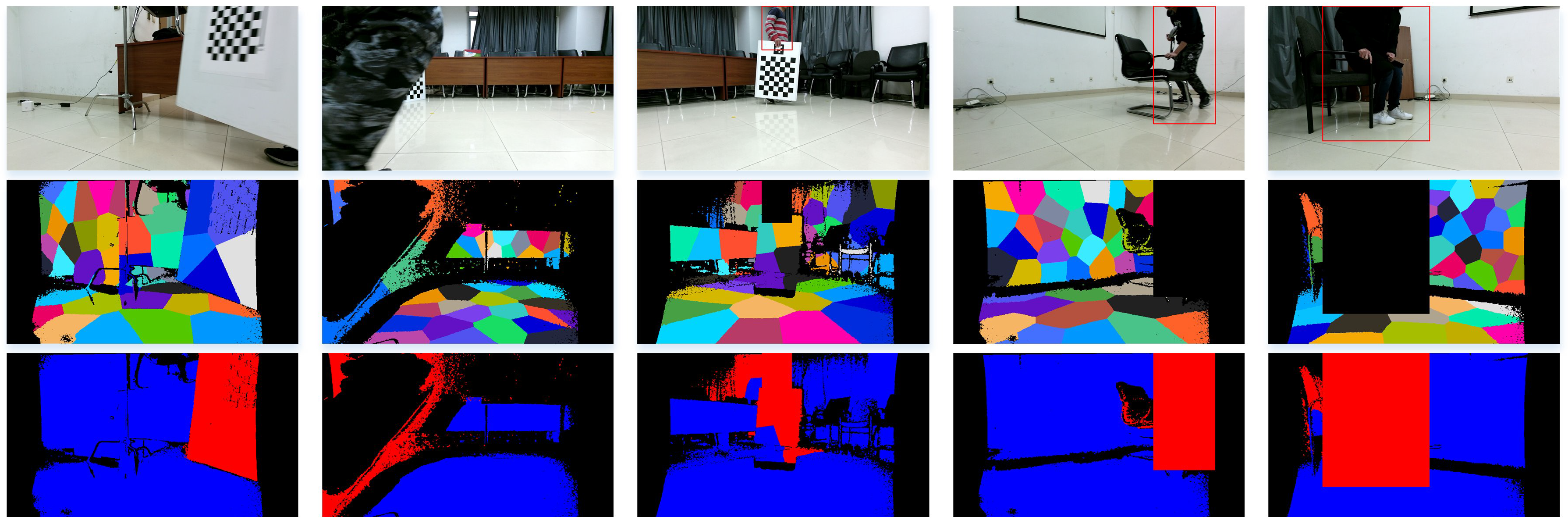
Figure 12 gives the results of the dynamic pixels culling module. In addition to predefined dynamic objects, such as persons, undefined moving objects, such as tablets and chairs, are also in the environments. YOLOv3 can recognize most predefined objects, but partially visible objects may not be identified (see the second column in Figure 12). Thanks to the multiview constraint-based strategy, we can handle the leak-recognized and undefined moving objects (see the first column in Figure 12). However, our approach also produces erroneous detections. For example, in the third column of Figure 12, the pixels of a part of the moving tablet are identified as static pixels. Because these pixels and some pixels on the ground are classified into one cluster by the K-means algorithm, and the ground pixels are the majority, our method determines this cluster as static. This problem can be solved by increasing the number of clusters, but it also increases the computation consumption. Moreover, our method cannot detect slow moving undefined dynamic objects due to the use of a fixed threshold. This small amount of mistaken recognitions do not pose a severe problem for the OctoMap construction, because OctoMap uses a filter. Only if a voxel has been observed as an obstacle multiple times will the occupancy probability of the voxel be high enough to label the voxel occupied.

5.3. Extension Tests

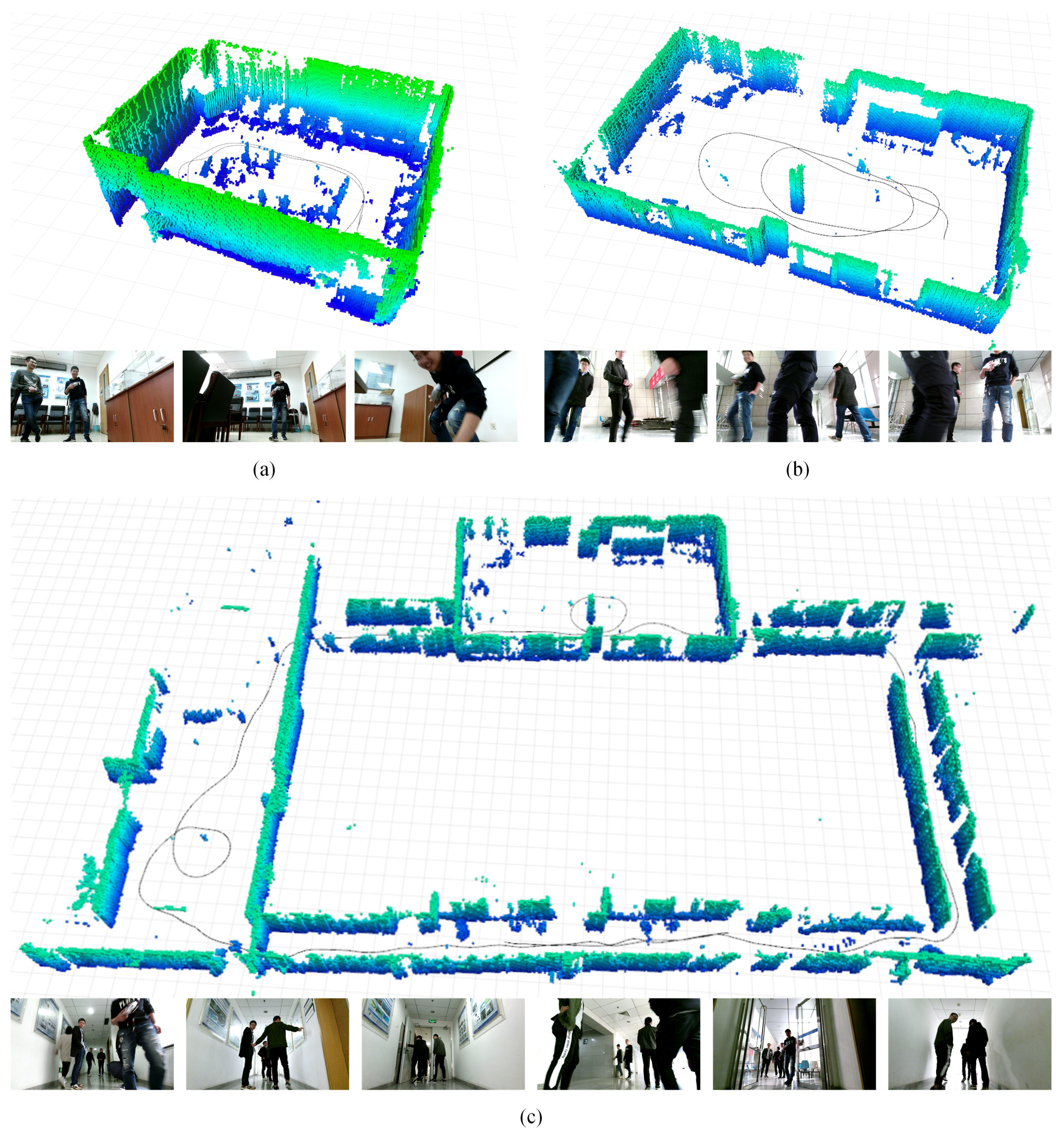
In this section, we further test the proposed system in an 8 m × 6 m office, a 15 m × 9 m hall, and a 37 m × 27 m corridor. In these sequences, several persons are moving at different speeds and directions. Many of them have only a part of their body in the view of the camera. Sometimes, the moving persons take up almost the entire field of view of the camera. There are some doors being opened and closed. These sequences are very challenging. Both the StaticFusion and Co-Fusion failed. Although RTAB-MAP can work, its trajectories and maps contain many twists. There are many dynamic objects be built in its maps. Conversely, DRE-SLAM successfully performs pose estimation, map construction, and loop closure, as shown in Figure 13. The robot trajectories are smooth and the maps hold no apparent distortions. Most dynamic objects are filtered out in the maps.

5.4. Performance of OctoMap Construction

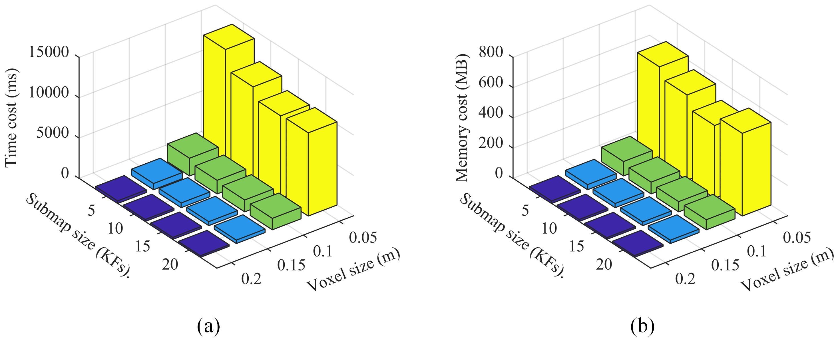
The voxel size and the submap size are two key parameters in our submap-based mapping algorithm. In this section, we experimentally explore the effects of these two parameters on the time cost, memory cost, and the quality of the map. We chose the longest sequence, i.e., the corridor, mentioned in Section 5.3, for this experiment. The DRE-SLAM has a loop of 408 keyframes in this sequence. We also compare our submap-based approach with the traditional retrace approach that rebuilds the entire map using all the raw data. We set four types of submap sizes, i.e., 5, 10, 15, and 20, and four types of voxel size, i.e., 0.05 m, 0.10 m, 0.15 m, and 0.20 m. We run DRE-SLAM a total of 16 times with the combinations of these different parameter configurations.

The time costs of the map update, when the loop has been closed, are shown in

Table 2. Time costs of the retrace approach and our method with various voxel sizes and submap size (ms).

Voxel Size (m)		Submap Size (KFs)
		5	10	15	20
0.05	Retrace	78,458.12	79,088.49	79,063.69	78,568.92
	Our approach	13,963.45	11,558.43	10,189.10	10,308.59
	Improvement	82.20%	85.39%	87.11%	86.88%
0.10	Retrace	12,754.71	12,607.22	12,712.09	12,730.30
	Our approach	2198.32	1682.83	1470.14	1416.18
	Improvement	82.76%	86.65%	88.44%	88.88%
0.15	Retrace	5476.40	5453.38	5549.65	5472.54
	Our approach	768.58	583.72	489.83	429.21
	Improvement	85.97%	89.30%	91.17%	92.16%
0.20	Retrace	3576.74	3694.08	3647.32	3728.31
	Our approach	324.03	238.94	246.99	196.73
	Improvement	90.94%	93.53%	93.23%	94.72%

and Figure 14a. Compared with the retrace method, our approach dramatically reduces the time consumption. The improvement rate is over $80\%$ in all the configurations. The improvement is more obvious when raising the voxel size or increasing the submap size. As seen from Figure 14a, the parameter that mainly influences the time cost is the voxel size. The submap size num has less effect. In other words, the time consumption will not increase too much when we choose a smaller submap size.

Table 3. Memory costs of the retrace approach and our method with various voxel sizes and submap sizes (MB).

Voxel Size (m)		Submap Size (KFs)
		5	10	15	20
0.05	Retrace	768.57	772.14	769.51	781.48
	Our approach	630.22	562.91	479.58	546.55
	Improvement	18.00%	27.10%	37.68%	30.06%
0.10	Retrace	770.69	768.68	773.55	773.81
	Our approach	95.24	77.92	67.56	66.47
	Improvement	87.64%	89.86%	91.27%	91.41%
0.15	Retrace	776.46	771.22	771.98	782.25
	Our approach	33.73	27.44	23.88	22.34
	Improvement	95.66%	96.44%	96.91%	97.14%
0.20	Retrace	770.64	770.67	772.14	772.39
	Our approach	16.52	13.04	11.55	11.01
	Improvement	97.86%	98.31%	98.50%	98.57%

and Figure 14b show the memory costs. In our approach, all the sub-OctoMaps and a full OctoMap are maintained in the memory. In the retrace approach, all the point clouds in all keyframes and a full OctoMap are stored in the memory. The full OctoMaps of the two methods are the same, which are not considered. We only calculate the memory needed to save the sub-OctoMaps for our approach and the point clouds for the retrace method. We assume one point occupies three float type of memory to count the memory of the point clouds. The function, memoryUsage(), provided by the OctoMap library is used to calculate the memory consumption of all the sub-OctoMaps. For configurations with a voxel size of 0.05 m, our method does not significantly improve the memory consumption. However, for configurations with resolutions of 0.10 m, 0.15 m, and 0.20 m, our algorithm dramatically reduces the memory consumption. The improvement rate is over $85\%$. This improvement is getting better with increasing the voxel size or increasing the submap size. As seen in Figure 14b, the voxel size plays a major role in the memory consumption, whereas the submap size has less impact. In summary, our approach effectively reduces the time cost and memory consumption. Furthermore, we can choose a smaller submap size without a significant increase in time and memory consumption.

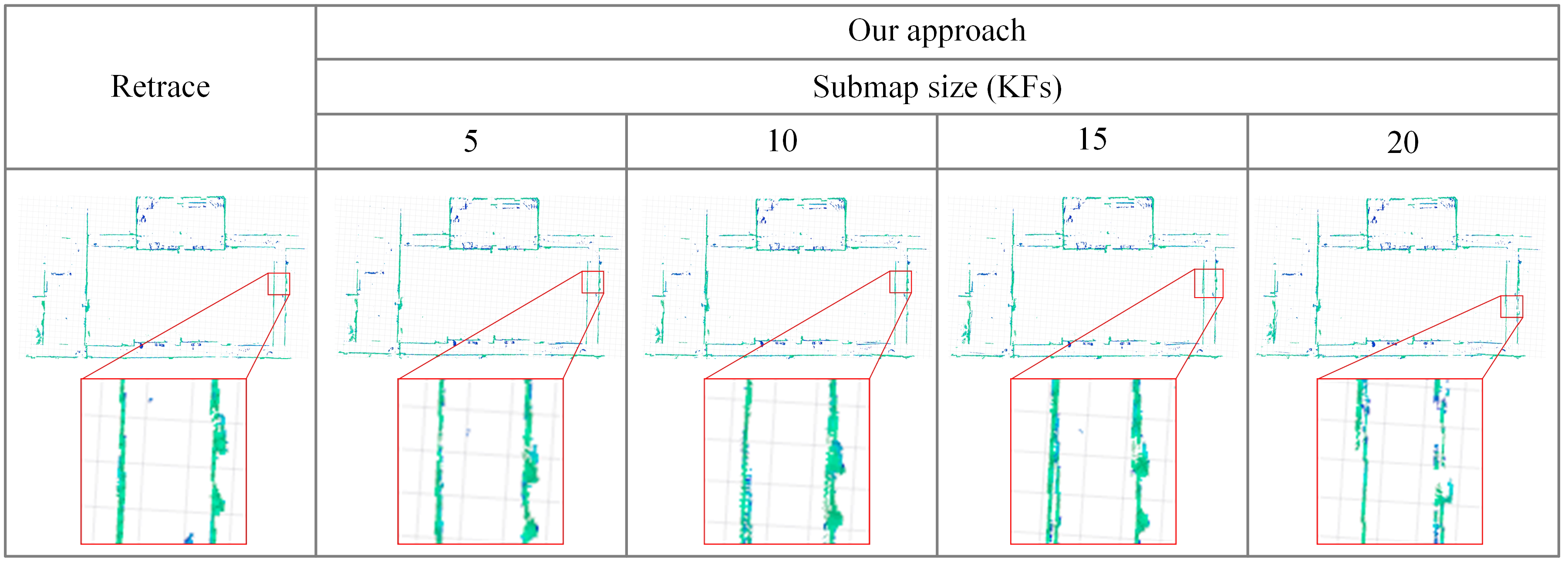
Figure 15 compares the map of retrace with the maps of our method in different submap sizes. The voxel size of the maps is 0.05 m. It can be seen that as the submap size increases, the distortion of the map tends to become larger. This is because the error of the sub-OctoMap increases with the submap size. There are no visible differences between our map with the retrace map when the submap size is 5. Combined with the above findings, we recommend setting the submap size to 5 and the voxel size to 0.1 m to obtain a balanced mapping performance.

5.5. Timing Results

Table 4. Timing results of each thread in milliseconds (mean ± STD).

Thread	Operation	Time Cost (ms)
RGB-D Encoder Tracking	Encoder integration	0.01 ± 0.00
	Feature extraction (1600 per frame)	17.28 ± 6.91
	3D–2D match	8.24 ± 4.48
	Pose estimation	5.86 ± 3.64
	Total	33.24 ± 12.12
Dynamic Pixels Culling	Object detection	162.17 ± 8.88
	K-means	286.71 ± 48.61
	Multiview constraints	28.10 ± 14.58
	Total	480.08 ± 54.27
Local Sparse Mapping	New map points creation	0.23 ± 0.06
	Local BA (Window size: 8 KFs)	138.54 ± 73.80
	Total	138.94 ± 73.83
Loop Closure (Loop size: 408 KFs)	Loop check	80.87
	Pose graph optimization	143.28
	Total	224.19
Sub-OctoMap Construction (voxel: 0.1 m)	Total	52.04 ± 27.84
Sub-OctoMap Fusion (408 KFs; voxel: 0.1 m)	Total	2198.32

presents the time costs of the DRE-SLAM. These time costs are calculated from the results of all the extension test sequences in Section 5.3. Our method costs approximately 34 ms per frame in the tracking part, in which the ORB feature extraction costs approximately 17 ms. The dynamic pixel culling takes approximately 480 ms per frame, in which the time costs of the object detection and the K-means segmentation are the majority. Due to the existence of dynamic objects, the number of map points participating in the local BA may vary greatly, so the time consumption of the Local BA has a large standard deviation. The loop closure detection time consumption is related to the number of keyframes in the loop. We provide the time result of the longest loop in the corridor sequence. The time costs in Table 4 are calculated in the dynamic scenes, which are smaller than the time costs in static scenes because less static map points and features can be used in the dynamic scenes. The tracking time is approximately 45 ms in static environments.

6. Conclusions

In this paper, we propose the dynamic RGB-D Encoder SLAM system, i.e., DRE-SLAM. The system works robustly and with high accuracy both in dynamic and static environments. DRE-SLAM takes measurements of an RGD-camera and two wheel-encoders as inputs and produces robot poses and a static background OctoMap. The system runs purely on a CPU, with no need for GPUs. The robustness and accuracy achieved are attributed to the tightly coupled approach with the encoders and the RGB-D camera. By combining the YOLOv3 object detection method with the multiview constraint-based method, we identify dynamic pixels on not only predefined dynamic objects but also undefined dynamic objects. The capability of working in dynamic environments is gained by culling the pixels occupied by these dynamic objects. The submap-based OctoMap construction approach significantly lowers the rebuilding time and memory consumption. We further find that the number of keyframes used to construct sub-OctoMaps has little effect on time and memory costs. Thus, we can reduce the number of keyframes in a submap to decrease the map distortion without adding too much computation and memory burdens. The proposed system is especially suitable for mobile robots that are operating in indoor dynamic environments.

In future work, we will extend our system in two directions. First, we will deal with the problem of wheel slipping to improve the robustness and accuracy. Second, we will explore the function of tracking dynamic objects.

References

- Mur-Artal, R.; Tardós, J.D. Orb-slam2: An open-source slam system for monocular, stereo, and rgb-d cameras. IEEE Trans. Robot. 2017, 33, 1255–1262. [Google Scholar] [CrossRef]
- Whelan, T.; Salas-Moreno, R.F.; Glocker, B.; Davison, A.J.; Leutenegger, S. Elasticfusion: Real-time dense slam and light source estimation. Int. J. Robot. Res. 2016, 35, 1697–1716. [Google Scholar] [CrossRef]
- Fu, X.; Zhu, F.; Wu, Q.; Sun, Y.; Lu, R.; Yang, R. Real-Time Large-Scale Dense Mapping with Surfels. Sensors 2018, 18, 1493. [Google Scholar] [CrossRef] [PubMed]
- Cadena, C.; Carlone, L.; Carrillo, H.; Latif, Y.; Scaramuzza, D.; Neira, J.; Reid, I.; Leonard, J.J. Past, present, and future of simultaneous localization and mapping: Toward the robust-perception age. IEEE Trans. Robot. 2016, 32, 1309–1332. [Google Scholar] [CrossRef]
- Qin, T.; Li, P.; Shen, S. Vins-mono: A robust and versatile monocular visual-inertial state estimator. IEEE Trans. Robot. 2018, 34, 1004–1020. [Google Scholar] [CrossRef]
- Yu, C.; Liu, Z.; Liu, X.-J.; Xie, F.; Yang, Y.; Wei, Q.; Fei, Q. Ds-slam: A semantic visual slam towards dynamic environments. In Proceedings of the IEEE/RSJ International Conference on Intelligent Robots and Systems (IROS), Madrid, Spain, 1–5 October 2018; pp. 1168–1174. [Google Scholar]
- Rünz, M.; Agapito, L. Co-fusion: Real-time segmentation, tracking and fusion of multiple objects. In Proceedings of the IEEE International Conference on Robotics and Automation(ICRA), Singapore, 29 May–3 June 2017; pp. 4471–4478. [Google Scholar]
- Bârsan, I.A.; Liu, P.; Pollefeys, M.; Geiger, A. Robust dense mapping for large-scale dynamic environments. In Proceedings of the IEEE International Conference on Robotics and Automation (ICRA), Brisbane, Australia, 21–25 May 2018; pp. 7510–7517. [Google Scholar]
- Bescos, B.; Fácil, J.M.; Civera, J.; Neira, J. Dynaslam: Tracking, mapping and inpainting in dynamic scenes. In Proceedings of the IEEE/RSJ International Conference on Intelligent Robots and Systems (IROS), Madrid, Spain, 1–5 October 2018. [Google Scholar]
- Rünz, M.; Agapito, L. Maskfusion: Real-time recognition, tracking and reconstruction of multiple moving objects. In Proceedings of the IEEE International Symposium on Mixed and Augmented Reality (ISMAR), Munich, Germany, 16–20 October 2018. [Google Scholar]
- Zhou, G.; Bescos, B.; Dymczyk, M.; Pfeiffer, M.; Neira, J.; Siegwart, R. Dynamic objects segmentation for visual localization in urban environments. arXiv, 2018; arXiv:1807.02996. [Google Scholar]
- Pizzoli, M.; Forster, C.; Scaramuzza, D. Remode: Probabilistic, monocular dense reconstruction in real time. In Proceedings of the IEEE/RSJ International Conference on Intelligent Robots and Systems, Chicago, IL, USA, 14–18 September 2014; pp. 2609–2616. [Google Scholar]
- Newcombe, R.A.; Izadi, S.; Hilliges, O.; Molyneaux, D.; Kim, D.; Davison, A.J.; Kohi, P.; Shotton, J.; Hodges, S.; Fitzgibbon, A. Kinectfusion: Real-time dense surface mapping and tracking. In Proceedings of the IEEE International Symposium on Mixed and Augmented Reality (ISMAR), Basel, Switzerland, 26–29 October 2011; pp. 127–136. [Google Scholar]
- Hornung, A.; Wurm, K.M.; Bennewitz, M.; Stachniss, C.; Burgard, W. Octomap: An efficient probabilistic 3d mapping framework based on octrees. Auton. Robots 2013, 34, 189–206. [Google Scholar] [CrossRef]
- Labbé, M.; Michaud, F. Rtab-map as an open-source lidar and visual simultaneous localization and mapping library for large-scale and long-term online operation. J. Field Robot. 2018, 36, 416–446. [Google Scholar] [CrossRef]
- Laidlow, T.; Bloesch, M.; Li, W.; Leutenegger, S. Dense rgb-d-inertial slam with map deformations. In Proceedings of the IEEE/RSJ International Conference on Intelligent Robots and Systems (IROS), Vancouver, BC, Canada, 24–28 September 2017; pp. 6741–6748. [Google Scholar]
- Scona, R.; Jaimez, M.; Petillot, Y.R.; Fallon, M.; Cremers, D. Staticfusion: Background reconstruction for dense rgb-d slam in dynamic environments. In Proceedings of the IEEE International Conference on Robotics and Automation (ICRA), Brisbane, Australia, 21–25 May 2018; pp. 1–9. [Google Scholar]
- Kim, D.-H.; Kim, J.-H. Effective background model-based rgb-d dense visual odometry in a dynamic environment. IEEE Trans. Robot. 2016, 32, 1565–1573. [Google Scholar] [CrossRef]
- Sun, Y.; Liu, M.; Meng, M.Q.-H. Improving rgb-d slam in dynamic environments: A motion removal approach. Robot. Auton. Syst. 2017, 89, 110–122. [Google Scholar] [CrossRef]
- Xiao, Z.; Dai, B.; Wu, T.; Xiao, L.; Chen, T. Dense scene flow based coarse-to-fine rigid moving object detection for autonomous vehicle. IEEE Access 2017, 5, 23492–23501. [Google Scholar] [CrossRef]
- Alcantarilla, P.F.; Yebes, J.J.; Almazán, J.; Bergasa, L.M. On combining visual slam and dense scene flow to increase the robustness of localization and mapping in dynamic environments. In Proceedings of the IEEE International Conference on Robotics and Automation (ICRA), Saint Paul, MN, USA, 14–18 May 2012; pp. 1290–1297. [Google Scholar]
- Wang, Y.; Huang, S. Towards dense moving object segmentation based robust dense rgb-d slam in dynamic scenarios. In Proceedings of the International Conference on Control Automation Robotics & Vision (ICARCV), Singapore, 10–12 December 2014; pp. 1841–1846. [Google Scholar]
- Besl, P.; Mckay, N. A method for registration of 3D shapes. IEEE Trans. Pattern Anal. Mach. Intell. 1992, 14, 239–256. [Google Scholar] [CrossRef]
- Curless, B.; Levoy, M. A volumetric method for building complex models from range images. In Proceedings of the 23rd Annual Conference on Computer Graphics and Interactive Techniques, New Orleans, LA, USA, 4–9 August 1996; pp. 303–312. [Google Scholar]
- Nießner, M.; Zollhöfer, M.; Izadi, S.; Stamminger, M. Real-time 3d reconstruction at scale using voxel hashing. ACM Trans. Graph. 2013, 32, 169. [Google Scholar] [CrossRef]
- Whelan, T.; Kaess, M.; Johannsson, H.; Fallon, M.; Leonard, J.J.; McDonald, J. Real-time large-scale dense rgb-d slam with volumetric fusion. Int. J. Robot. Res. 2015, 34, 598–626. [Google Scholar] [CrossRef]
- Endres, F.; Hess, J.; Sturm, J.; Cremers, D.; Burgard, W. 3D mapping with an rgb-d camera. IEEE Trans. Robot. 2014, 30, 177–187. [Google Scholar] [CrossRef]
- He, K.; Gkioxari, G.; Dollar, P.; Girshick, R. Mask r-cnn. In Proceedings of the IEEE International Conference on Computer Vision (ICCV), Venice, Italy, 22–29 October 2017; pp. 2980–2988. [Google Scholar]
- Badrinarayanan, V.; Kendall, A.; Cipolla, R. Segnet: A deep convolutional encoder-decoder architecture for image segmentation. IEEE Trans. Pattern Anal. Mach. Intell. 2017, 39, 2481–2495. [Google Scholar] [CrossRef] [PubMed]
- Newcombe, R.A.; Fox, D.; Seitz, S.M. Dynamicfusion: Reconstruction and tracking of non-rigid scenes in real-time. In Proceedings of the IEEE Conference on Computer Vision and Pattern Recognition (CVPR), Boston, MA, USA, 7–12 June 2015; pp. 343–352. [Google Scholar]
- Dou, M.; Khamis, S.; Degtyarev, Y.; Davidson, P.; Fanello, S.R.; Kowdle, A.; Escolano, S.O.; Rhemann, C.; Kim, D.; Taylor, J. Fusion4d: Real-time performance capture of challenging scenes. ACM Trans. Graph. 2016, 35, 114. [Google Scholar] [CrossRef]
- Bi, S.; Yang, D.; Cai, Y. Automatic Calibration of Odometry and Robot Extrinsic Parameters Using Multi-Composite-Targets for a Differential-Drive Robot with a Camera. Sensors 2018, 18, 3097. [Google Scholar] [CrossRef] [PubMed]
- Siegwart, R.; Nourbakhsh, I.R. Introduction to Autonomous Mobile Robots, 2nd ed.; MIT Press: Cambridge, MA, USA, 2004; pp. 270–275. [Google Scholar]
- Redmon, J.; Farhadi, A. Yolov3: An incremental improvement. arXiv, 2018; arXiv:1804.02767. [Google Scholar]
- Lin, T.-Y.; Maire, M.; Belongie, S.; Hays, J.; Perona, P.; Ramanan, D.; Dollár, P.; Zitnick, C.L. Microsoft coco: Common objects in context. In Proceedings of the European Conference on Computer Vision (ECCV), Zurich, Switzerland, 6–12 September 2014; pp. 740–755. [Google Scholar]
- Gálvez-López, D.; Tardos, J.D. Bags of binary words for fast place recognition in image sequences. IEEE Trans. Robot. 2012, 28, 1188–1197. [Google Scholar] [CrossRef]
- Ceres Solver. Available online: http://ceres-solver.org (accessed on 15 January 2019).
- Rosbag. Available online: http://wiki.ros.org/rosbag (accessed on 15 January 2019).
- iai_kinect2. Available online: https://github.com/code-iai/iai_kinect2/ (accessed on 15 January 2019).
- Garrido-Jurado, S.; Muñoz-Salinas, R.; Madrid-Cuevas, F.J.; Marín-Jiménez, M.J. Automatic generation and detection of highly reliable fiducial markers under occlusion. Pattern Recognit. 2014, 47, 2280–2292. [Google Scholar] [CrossRef]
- Hartley, R.; Zisserman, A. Multiple View Geometry in Computer Vision, 2nd ed.; Cambridge University Press: Cambridge, UK, 2003; pp. 87–131. [Google Scholar]
- evo. Available online: https://michaelgrupp.github.io/evo/ (accessed on 15 January 2019).
Figure 1.
Differential-drive robot equipped with an RGB-D camera.
Figure 2.
Pipeline of the proposed DRE-SLAM.
Figure 3.
Principle of matching of the local map points with the ORB features.
Figure 4.
Pipeline of dynamic pixels culling.
Figure 5.
An illustration of the local bundle adjustment.
Figure 6.
An illustration of the OctoMap construction. (a) sub-OctoMaps, (b) full OctoMap.
Figure 7.
RedBot, Kinect 2.0 camera, and ground truth acquisition device.
Figure 8.
Experimental environments and RGB images in the static, low dynamic, and high dynamic data sequences.
Figure 9.
The root-mean-square-error (RMSE) of (a) the translation (m) and (b) the rotation (rad) comparison of the four methods in all the sequences.
Figure 10.
Comparison of the trajectories of the proposed method with the ground truth in the (a) office, (b) lab, and (c) corridor environments. The absolute pose errors are encoded by colors.
Figure 11.
Maps obtained by the four methods in the (a) office, (b) lab, and (c) corridor environments. The red circles show the deformation and the dynamic data introduced in the OctoMaps created by RTAB-MAP.
Figure 12.
Typical results of the dynamic pixels culling module. The first row includes the predefined dynamic object detection results. The second row includes the results of K-means segmentation using the depth images. The third row shows the final dynamic pixel detection results. The red pixels are dynamic, the blue pixels are static, and the black pixels are pixels with invalided depth values.
Figure 13.
Results of the extension tests. (a) 8 m × 6 m office (Voxel size: 0.05 m), (b) 15 m × 9 m hall (Voxel size: 0.05 m), and (c) 37 m × 27 corridor (Voxel size: 0.1 m). The black lines are the robot trajectories of keyframes.
Figure 14.
(a) time cost and (b) memory cost of our approach with various voxel sizes and submap sizes.
Figure 15.
Top view of a map built by the retrace approach and top views of maps built by our approach with different submap sizes. The voxel size is 0.05 m.