Mitigation of Tropospheric Delay in SAR and InSAR Using NWP Data: Its Validation and Application Examples

1
Previously with Technische Universität München, Arcisstr. 21, D-80333 Munich, Germany
2
Currently with ADC Automotive Distance Control Systems GmbH, Peter-Dornier-Str. 10, D-88131 Lindau, Germany
3
DLR, Remote Sensing Technology Institute, Muenchener Str. 20, D-82234 Wessling, Germany
*
Author to whom correspondence should be addressed.
Remote Sens. 2018, 10(10), 1515; https://doi.org/10.3390/rs10101515
Submission received: 17 July 2018
/
Revised: 8 September 2018
/
Accepted: 11 September 2018
/
Published: 21 September 2018
(This article belongs to the Special Issue Ten Years of TerraSAR-X—Scientific Results)
Abstract
:The neutral atmospheric delay has a great impact on synthetic aperture radar (SAR) absolute ranging and on differential interferometry. In this paper, we demonstrate its effective mitigation by means of the direction integration method using two products from the European Centre for Medium-Range Weather Forecast: ERA-Interim and operational data. Firstly, we shortly review the modeling of the neutral atmospheric delay for the direct integration method, focusing on the different refractivity models and constant coefficients available. Secondly, a thorough validation of the method is performed using two approaches. In the first approach, numerical weather prediction (NWP) derived zenith path delay (ZPD) is validated against ZPD from permanent GNSS (global navigation satellite system) stations on a global scale, demonstrating a mean accuracy of 14.5 mm for ERA-Interim. Local analysis shows a 1 mm improvement using operational data. In the second approach, NWP derived slant path delay (SPD) is validated against SAR SPD measured on corner reflectors in more than 300 TerraSAR-X High Resolution SpotLight acquisitions, demonstrating an accuracy in the centimeter range for both ERA-Interim and operational data. Finally, the application of this accurate delay estimate for the mitigation of the impact of the neutral atmosphere on SAR absolute ranging and on differential interferometry, both for individual interferograms and multi-temporal processing, is demonstrated.
1. Introduction
The atmosphere affects the propagation of radar signals and causes delays in the range direction. There are two main effects: the dispersive delay caused by the ionosphere and the neutral delay caused mainly by the lower atmosphere. The first effect depends on the radar frequency and has an impact of several centimeters in X-band. Fortunately, this effect can be determined and compensated efficiently using total electron content (TEC) maps based on multi-frequency measurements from regional/global networks of global navigation satellite system (GNSS) [1,2] or using the split-spectrum method in interferograms [3,4]. The neutral atmospheric delay has an average value in the meter range and exhibits variations over space and time in the decimeter-level. It is thus mandatory to mitigate it in order to derive accurate absolute and/or relative synthetic aperture radar (SAR) range measurements.
Several methods have been developed for the mitigation of the neutral atmospheric delay exploiting external measurements. In [5,6], the delay is approximated using surface meteorological measurements, achieving an accuracy of several decimeters. The main limitation of such ground-based techniques as well as those based on space-borne water vapor measurements is the sparse spatial and temporal distribution of data [7,8]. Therefore, several methods based on regional or global numerical weather prediction (NWP) products have been proposed [9,10]. In [11,12,13], meso-scale weather models are applied with input from NWP data in order to simulate the weather situation at the exact acquisition time and with a higher spatial resolution. Their accuracy depends on the quality of the input NWP data and varies from centimeter to decimeter range.
The integration method has been introduced in [10,14,15]. It calculates the neutral atmospheric delay using global reanalysis data provided by the European Centre for Medium-Range Weather Forecasts (ECMWF). Its absolute accuracy has been validated against GPS zenith path delay (ZPD) measurements. In [14,15] the application of global NWP products to mitigate neutral atmospheric delay effects in InSAR measurement has been demonstrated. In both studies, the neutral atmospheric delay was firstly integrated in the zenith direction and then projected in the slant direction. In contrast, the direct integration method introduced in [10] integrates the refractivity along the actual propagation path of the radar echoes.
In this paper we focus on two aspects: firstly, a validation of the integrated delay using global NWP products and, secondly, an analysis of the impact of the neutral atmospheric delay on absolute range measurements and differential interferometry and its mitigation. The paper is organized in five sections. In Section 2, the methodology is introduced, discussing the different models and their coefficients. The validation experiments are presented in Section 3. In Section 4 the applications are demonstrated: firstly for absolute ranging measurements and secondly for interferometric measurements. Finally, a short conclusion is provided in Section 5.
2. Methodology
2.1. Atmospheric Path Delay in the Neutral Atmosphere
In the lower atmosphere (<80 km), gravitation and air pressure regulate the vertical atmospheric motion in a hydrostatic equilibrium. Under this condition, the troposphere tends to be stratified and air density is a function of temperature and pressure, which are themselves highly dependent on height. Their relationship can be expressed as Equation (1) [16]:
where P is pressure in Pascal (Pa); z is geometric height in meter (m); T is temperature in Kelvin (K); g is the gravitational acceleration; is a constant for 1 kg of an ideal gas, e.g., is the gas constant for 1 kg of dry air and the gas constant for 1 kg of water vapor; is the virtual temperature, which is used to derive the temperature lapse rate of moist air [16].
In this section, the air refractivity equation for the neutral atmosphere as well as its alternative expressions associated with different coefficient constants are presented. Based on the statistical analysis in Section 2.1.3, an approximated expression of air refractivity has been selected for delay integration.
2.1.1. Air Refractivity and Neutral Atmospheric Propagation Delay
The refractive index n varies along the radar echo propagation path. The refractivity describes the variation with respect to vacuum due to the atmosphere. For convenience, scaled-up refractivity is introduced. Neglecting non-ideal gas effects and the effect of the ionosphere, air refractivity N can be written as [17,18,19]:
where is the partial pressure of dry air in hPa; e is the partial pressure of water vapor in hPa; T is the absolute temperature in K; is the cloud water content in . The constants , and are derived from laboratory measurements and under different approximations, which are discussed in Section 2.1.3. Note that this equation does not account for the refractivity of the ionosphere, since it is not part of the neutral atmospheric delay.
2.1.2. Integration of the Neutral Atmospheric Delay and Its Alternative Expressions
The total neutral atmospheric delay can be defined as the difference between the radio path length and the straight-line distance [20], which is divided into two parts: the signal delay along the propagation path and the geometric delay due to the bending effect. In this paper, the ray-path bending effect is neglected due to the rather steep incidence angle (typically 20–45) of SAR acquisitions. Therefore, the neutral atmospheric delay is approximated as the integral of air refractivity along the straight-line path from Earth’s surface to the upper limit of the available NWP data. The integration in zenith direction and in slant direction can be expressed:
where is the height of Earth’s surface; represents the upper limit of the integration path; is the starting point of integration; indicates the end point of the integration path.
Different assumptions have been performed for different applications. Thus the integration has been formulated according to different expressions. Taking the integration in zenith direction as an example, three groups of expressions have been defined under the assumptions of: (1) ideal gases; (2) non-ideal gases; and (3) non-ideal gases based on an approximated equation. For each of them the zenith delay can be written as a combination of hydrostatic and wet delay :
- (1)
- ;
- (2)
- ;
- (3)
- .
For an ideal gas, the hydrostatic delay can be approximated as a function of surface pressure and the wet delay is given by the last two terms of Equation (3), thus
where is given by the last layer (first level) of the NWP product and is the mean gravity acceleration at the mass center of the atmospheric column. In [21] an approximate form for is provided as a function of latitude and geometric height z:
where the constant is equal to . For non-ideal gases, according to Equation (4) the integration can be formulated be as:
where .
Finally an approximate non-ideal gas hydrostatic equation can be derived as
2.1.3. Coefficient Constants
The coefficient constants , and are empirical values which can be retrieved from laboratory experiments, such as in [18,22]. For geodetic applications, different sets of coefficient constants have been proposed in [21,23,24]. Recently, [19,25] suggest more accurate coefficient constants for precise geodetic applications and GPS radio occultation. The coefficient constants proposed in the literature for the different integral equations are summarized in Table 1. In order to compare them, the ZPD at the Wettzell GNSS station has been integrated for each of the available NWP products from August 2013, generating thus one delay every six hours for each of them. The ZPD integrated according to Equation (9) and the coefficient constants from [18] are used as reference. The mean value and the standard deviation of the residual ZPDs after compensating the reference ZPD are summarized in Table 1.
Regarding the statistical analysis of ZPD differences presented in Table 1, the mean value varies from to mm and the standard deviation from <0.1 mm to mm. In general, the reference ZPD is close to the ZPDs under the assumption of an ideal gas, since their standard deviations are all <0.5 mm. The minimum offset of mm is observed for the ideal gas using the same constants [18] as the reference ZPD. The maximum standard deviation ( mm) and mean value ( mm) are yielded by the approximated formula for non-ideal gases, been the difference to the reference ZPD thus caused by the different constant values. The next closest constants to [18] are provided by [19] under the assumption of an ideal gas, where the standard deviation is less than mm and the offset is about mm. In summary, for an ideal gas, the discrepancies in terms of mean value are mainly caused by the difference in ; for non-ideal gases, the differences are primarily induced by different formulae of the hydrostatic delay .
2.2. Direct Integration Method Using Global NWP Products
The direct integration method has been introduced in [10,26]. It has three processing steps: preprocessing and preparation, horizontal interpolation and direct integration. According to the input scene parameters, such as acquisition time, scene location and satellite orbit information, the corresponding NWP data sets are downloaded from the ECMWF product server. In the first step, the NWP products are preprocessed to a regular latitude-longitude grid and each model level is related to a geometrical height [27]. A proper horizontal interpolation is required due to the coarse horizontal resolution of NWP data. Finally, the integration starts from a given location (for instance, a GPS receiver or a SAR image pixel) and ends at the top of NWP data. The meteorological parameters at each integration step are interpolated or extrapolated along the integration path in zenith or in slant range direction in order to evaluate and integrate refractivity.
2.3. Terminology: Tropospheric Delay
The neutral atmospheric delay is integrated until the top level of the NWP data, which depending on the ECMWF product has a geometric altitude of approximately 65 km (0.2 hPa for ERA-Interim) (https://www.ecmwf.int/en/forecasts/documentation-and-support/60-model-levels) or 79 km (0.02 hPa for operational data) (https://www.ecmwf.int/en/forecasts/documentation-and-support/137-model-levels). Thus the integration is performed across the troposphere, the stratosphere and the mesosphere. Commonly, in the SAR community this neutral atmospheric delay is called tropospheric delay, since the troposphere has the highest contribution to the neutral atmospheric delay. In the following we will follow this convention, namely we will use the term tropospheric delay instead of neutral atmospheric delay.
3. Validation of Integrated Tropospheric Delay
3.1. ECMWF Products
In the last decades, major improvements in NWP accuracy have been achieved thanks mainly to increased computational power and increased observation coverage. Nowadays, the NWP models provide a variety of atmospheric parameters on a global scale with high horizontal and vertical resolution. It provides a unique possibility to derive the necessary 3-dimensional atmospheric parameters for delay integration at a given analysis time, namely P, T and e.
Two kinds of NWP products generated by the ECMWF Integrated Forecast System (IFS) have been selected for integration: reanalysis data sets and operational data (OP). Reanalysis data are produced with a fixed IFS version and at a fixed resolution. ERA-Interim is the current ECMWF global atmospheric reanalysis, providing data sets from 1979 up to a 3 months delay behind real time [28]. It will be fully replaced by ERA5 reanalysis by the end of 2018 [29], the next generation of reanalysis data set. ERA5 reanalysis products are available hourly compared to the 6-hour interval of ERA-Interim and OP. Reanalysis data sets can be accessed via the ECMWF public data service. The operational forecast based on the up-to-date IFS version enables a near real-time analysis with a wider range of atmospheric parameters only for registered users. The basic product specifications, such as horizontal and vertical resolution and IFS release cycle are presented in Table 2. The selection of NWP products depends on access authorization, data availability and the application.
In this study, both reanalysis and operational data are used. The validation is focused on ERA-Interim and OP. ERA-Interim data are downloaded from the ECMWF public data sets (http://apps.ecmwf.int/datasets/data/interim-full-daily/levtype=ml/). OP are acquired from archive catalogue.
3.2. Validation Approaches
The ECMWF IFS performs each data assimilation with millions of observations from an extensive range of inputs, which are not error-free. Therefore, it is important to determine the accuracy and the reliability of NWP products for the calculation of the integrated tropospheric delay. According to the air refractivity equation (Equation (10)), the accuracy of the delay depends on the accuracies of P, T and e. An overview of the general assessment of ERA-Interim products in comparison with GPS ZPD is provided in [28]. Compared to the accuracy of P and T, the accuracy of water vapor (related to e) is limited due to the modeling complexity and to the accuracy of the input data [30,31,32,33].
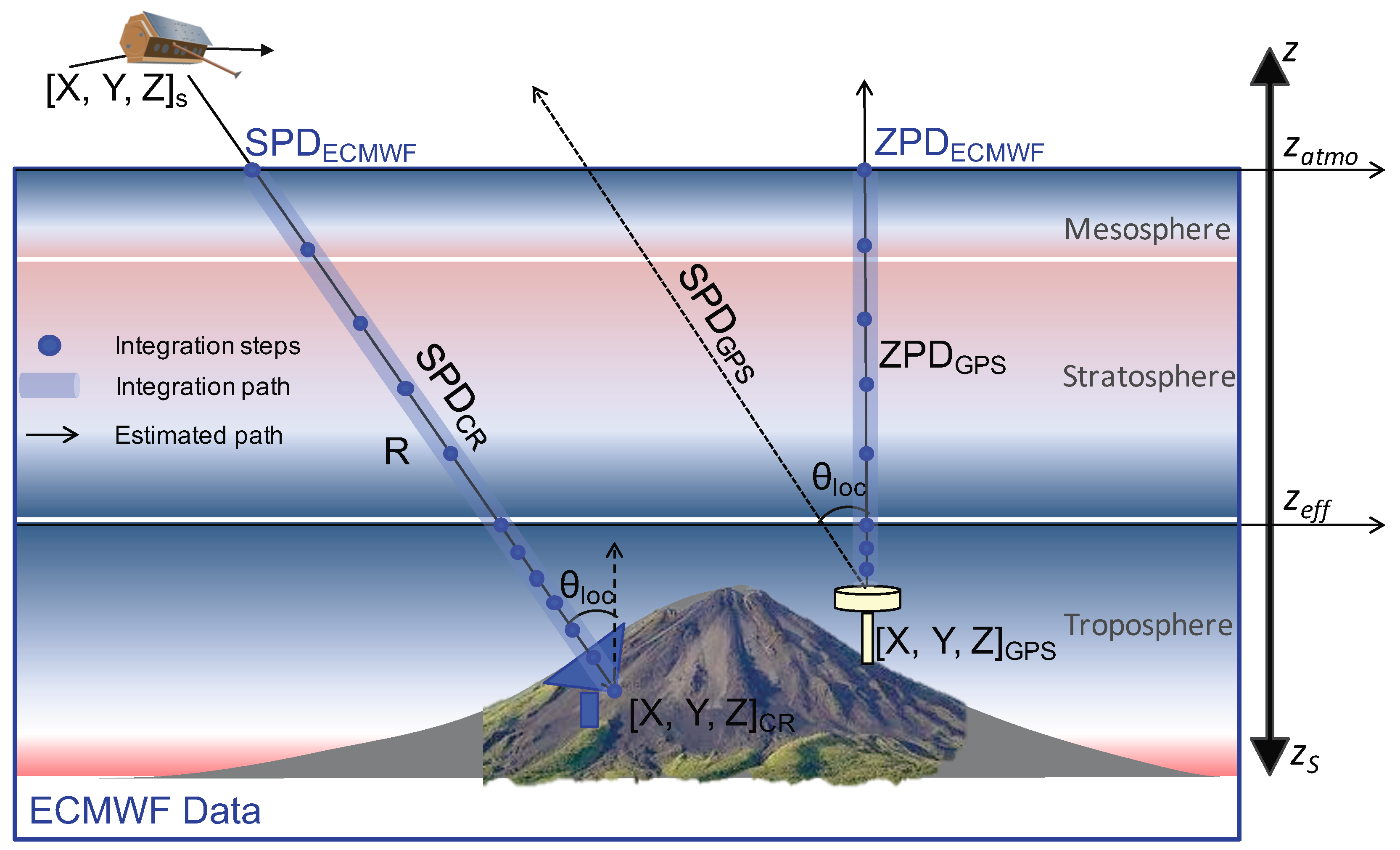
A validation approach is proposed in order to evaluate the accuracy of ECMWF integrated tropospheric delay using GPS and corner reflector (CR) observations as reference data sets. A sketch of the validation concept is depicted in Figure 1. The reference tropospheric delays are ZPD derived from GPS measurements () and SPD estimated from CR observations () using the Imaging Geodesy method [34]. The tropospheric delays are integrated both in zenith () and in slant range () direction using ECMWF products in order to compare them to the reference data sets. In Section 3.3, from both ERA-Interim and OP are compared to from the International GNSS Service (IGS) [35]. In Section 3.4, a comparison of from both ERA-Interim and OP with at two GNSS stations is presented.
3.3. Validation of Integrated ZPD with GPS ZPD
For precise positioning purposes the tropospheric delay must be estimated in the GPS analysis [21,23]. GPS ZPDs are not assimilated at the ECMWF [36]. Hence, ECMWF ZPDs are independent from GPS ZPDs. GPS ZPD has been widely used for comparison against the integrated total delay and/or the integrated delay of water vapor (ZWD) derived from radiosondes, microwave radiometers and NWP products [37,38,39]. The accuracy of GPS ZPD measurements has been proven to be of about 5 mm [38].
3.3.1. Time-Series Comparison Using ERA-Interim and OP Data Sets at the Wettzell Station
A time series of ECMWF ZPD has been generated using 1460 ERA-Interim and OP data fields at the Wettzell station in 2015. For validation purposes, the corresponding GPS ZPD time series has been gathered from IGS. Unfortunately, GPS ZPDs are not always available during this year. There is a 17 days data-gap. The single ECMWF ZPD for each analysis time (0, 6, 12 and 18 h UTC) is integrated from the station coordinates to the top of the NWP data. Furthermore, empirical ZPDs are calculated based on the GPT2w model [40].
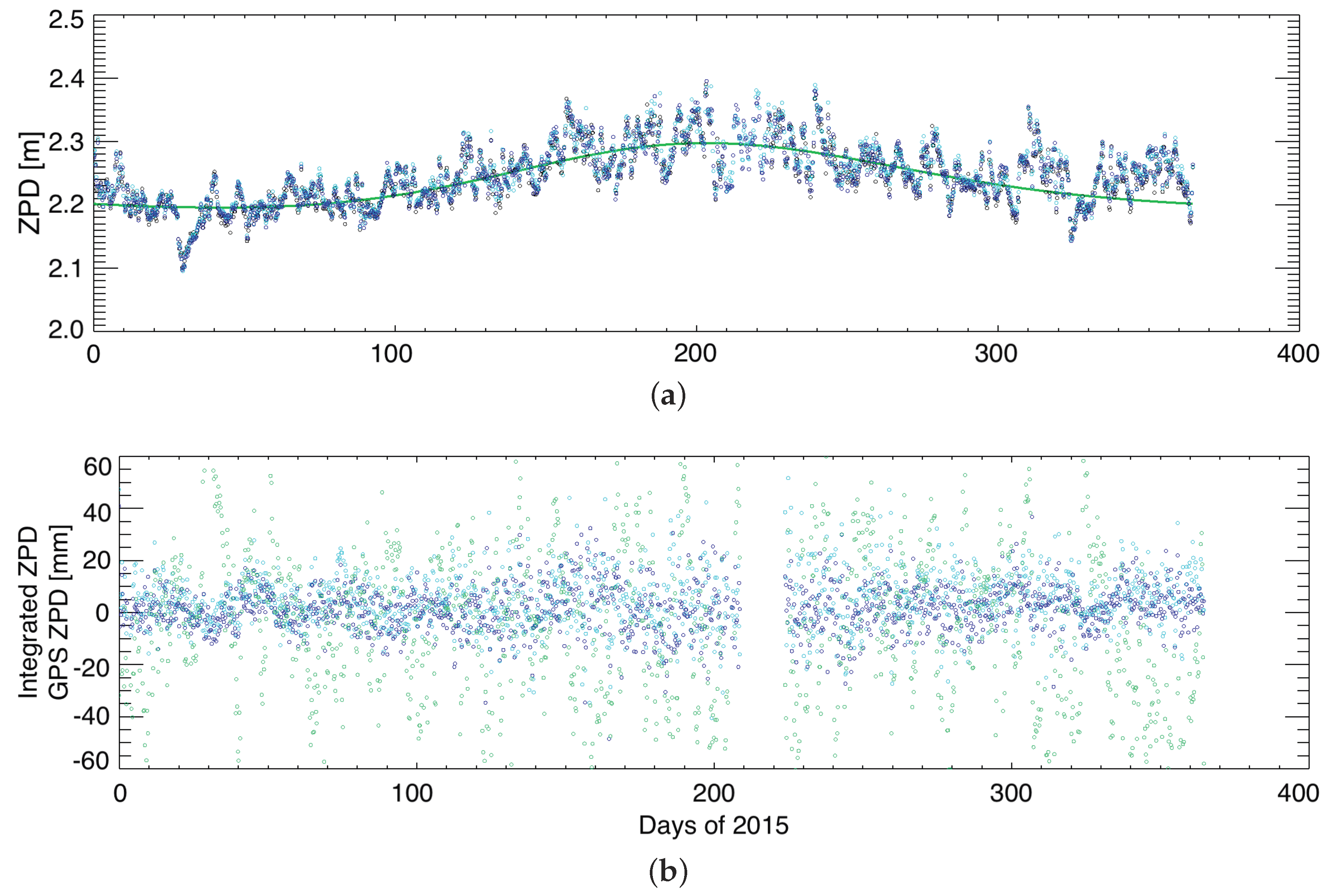
The comparison is presented in Figure 2. GPS ZPD varies about 29 cm along the year, from m in winter to m in summer. Both integrated ZPDs using ERA-Interim and OP exhibit a good agreement with GPS ZPD. The differences between integrated ZPDs and GPS ZPD are depicted in Figure 2b. The standard deviation of differences is about mm for ERA-Interim and mm for OP. The offsets are both under 5 mm, mm for ERA-Interim and mm for OP. The empirical model can capture the seasonal trend of the delay, but the standard deviation of the residual difference is mm, approximately three times higher than that of integrated delays.
3.3.2. Global Validation of ERA-Interim Products
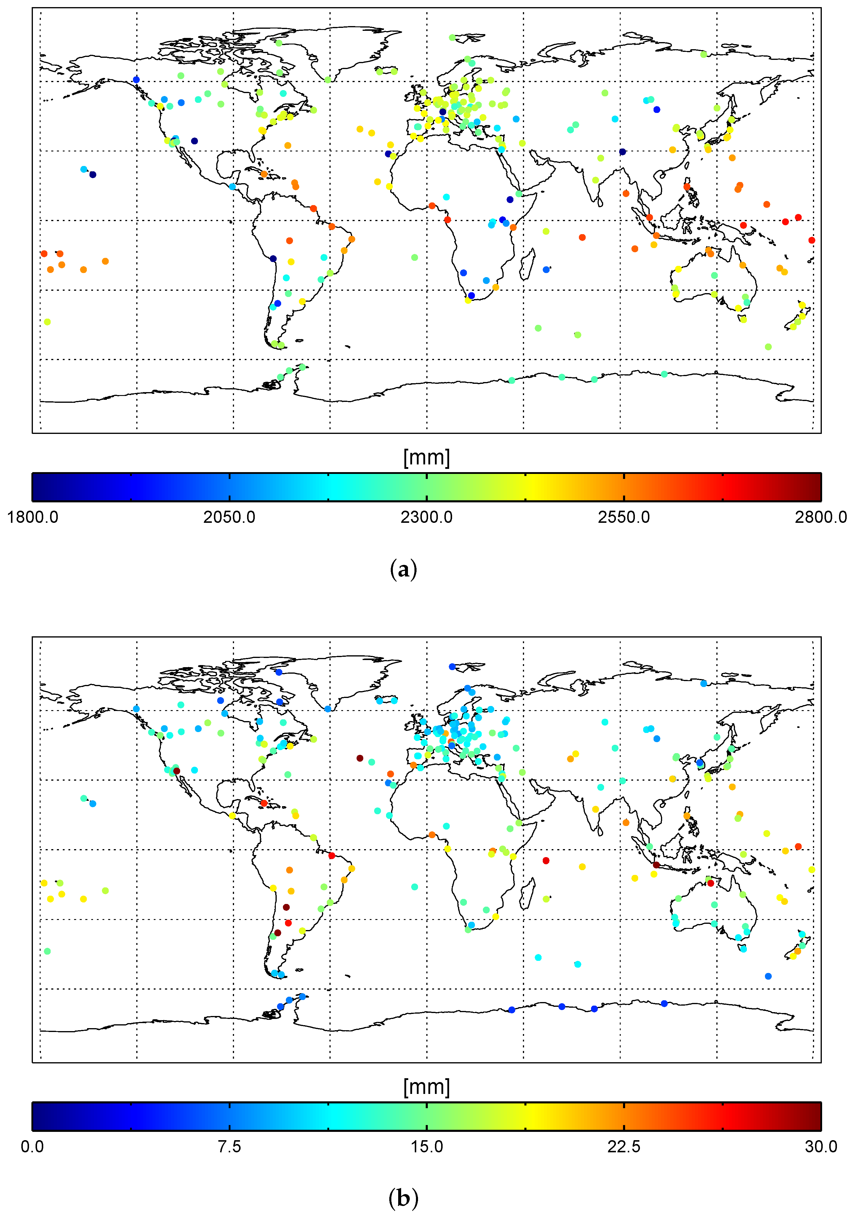
In order to test the quality of ECMWF products globally, the validation of ERA-Interim products is extended to a global scale using 268 permanent stations from the IGS network as reference. The time-series validation approach presented in Section 3.3.1 is carried out for the GPS stations of the IGS network over the time period from 2010 to 2015. The average value of the ZPD over time is presented in Figure 3a. The maximum delay is m and the minimum is m. The average over the 268 stations is m. The magnitude of the temporal variation of the delay can be represented by the standard deviation of the ZPD over time for a given station, which varies from mm to mm and has an average value over the stations of mm.
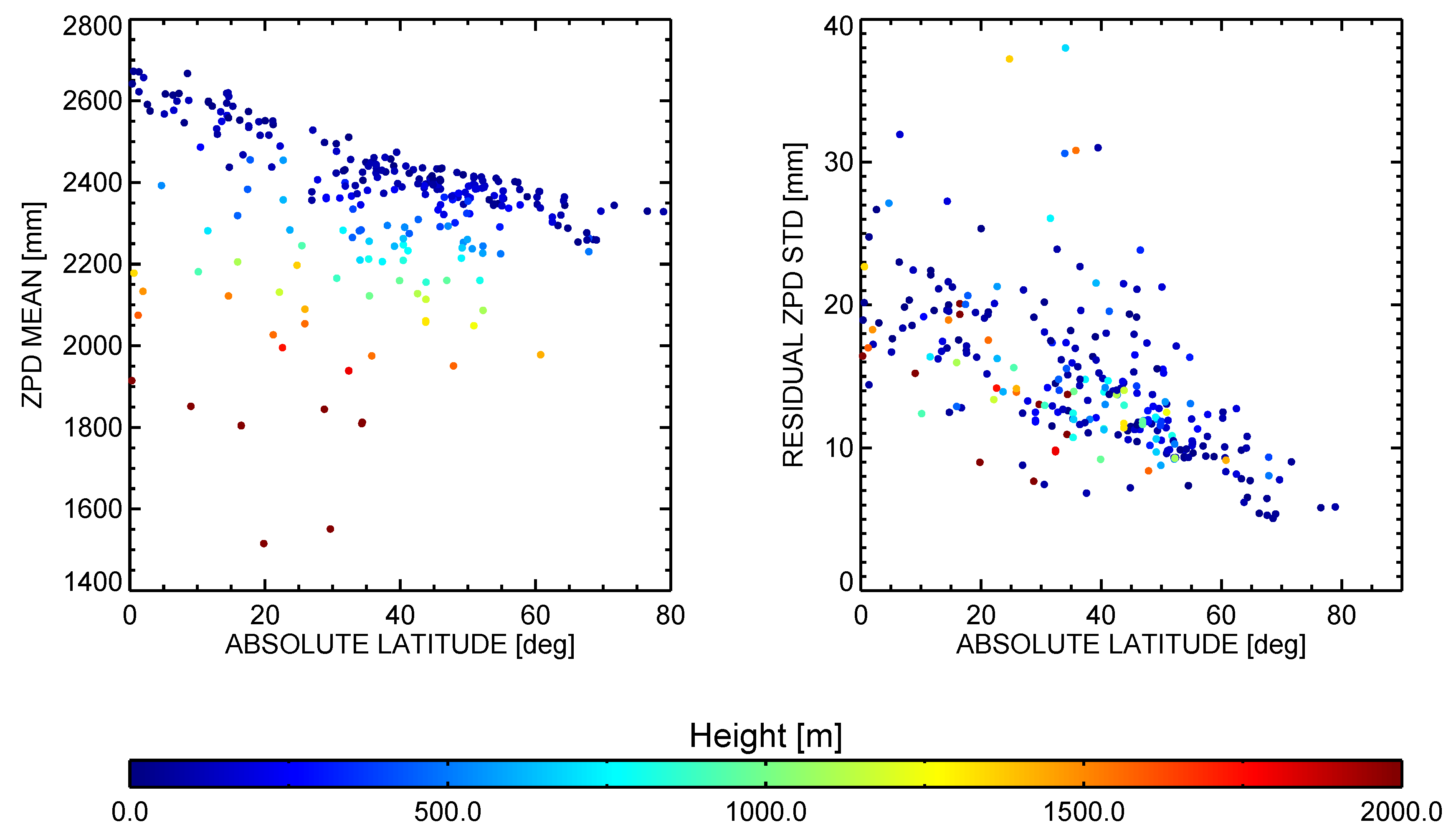
The difference between integrated ZPD and GPS ZPD is calculated in order to evaluate the accuracy of the ERA-Interim integrated delay. The standard deviation of the differences is depicted in Figure 3b. The average standard deviation over the 268 GPS stations is mm, with a minimum of mm and a maximum of mm. The accuracy of the integrated delay is directly related to the water vapor content distribution. In higher latitudes the water vapor content is lower than in lower latitudes due to the lower temperatures at higher latitudes [41]. In order to visualize this dependency of the integrated delay accuracy on latitude, a scatter plot with the absolute latitude as X-axis and the standard deviation of the difference as Y-axis is shown in Figure 4 (right) color coded according to the station height. The accuracy of the integrated delay in higher latitudes (>55) is better than cm. In lower latitudes (<), the accuracy is mostly between and cm due to the higher water vapor content. No obvious dependency on height can be observed. An analogous scatter plot for the mean integrated ZPD is shown in Figure 4 (left), where a clear dependency on absolute latitude as well as on height can be observed.
3.4. Validation of Integrated SPD with SPD Estimated from CR Measurements
As introduced in [34], the mismatch between the measured absolute range of a target in a SAR image and its predicted position (calculated using the orbit information and its known absolute position) is caused not only by the tropospheric delay and measurement noise, but also by the ionospheric delay as well as delays caused by geodetic effects, such as solid Earth tides (SET), ocean tidal loading (OTL), atmospheric pressure loading (APL) and continental drift (CD). Atmospheric (tropospheric and ionospheric) delays and geodetic effects must be considered in order to achieve centimeter-level ranging accuracy [1,26,34]. The tropospheric delay in SAR range measurements (SAR SPD) can be estimated if all the other effects have been accurately corrected for on the range mismatch. This SAR SPD can be used for validation of the ECMWF SPD. Furthermore, if there is a permanent GPS station nearby then the slant tropospheric delay GPS SPD, here calculated from the GPS ZPD using the secant of the SAR incidence angle as mapping function, can be used as an additional reference for validation. In this section, both SAR SPD and GPS SPD are used as reference for validation of the ECMWF integrated SPD.
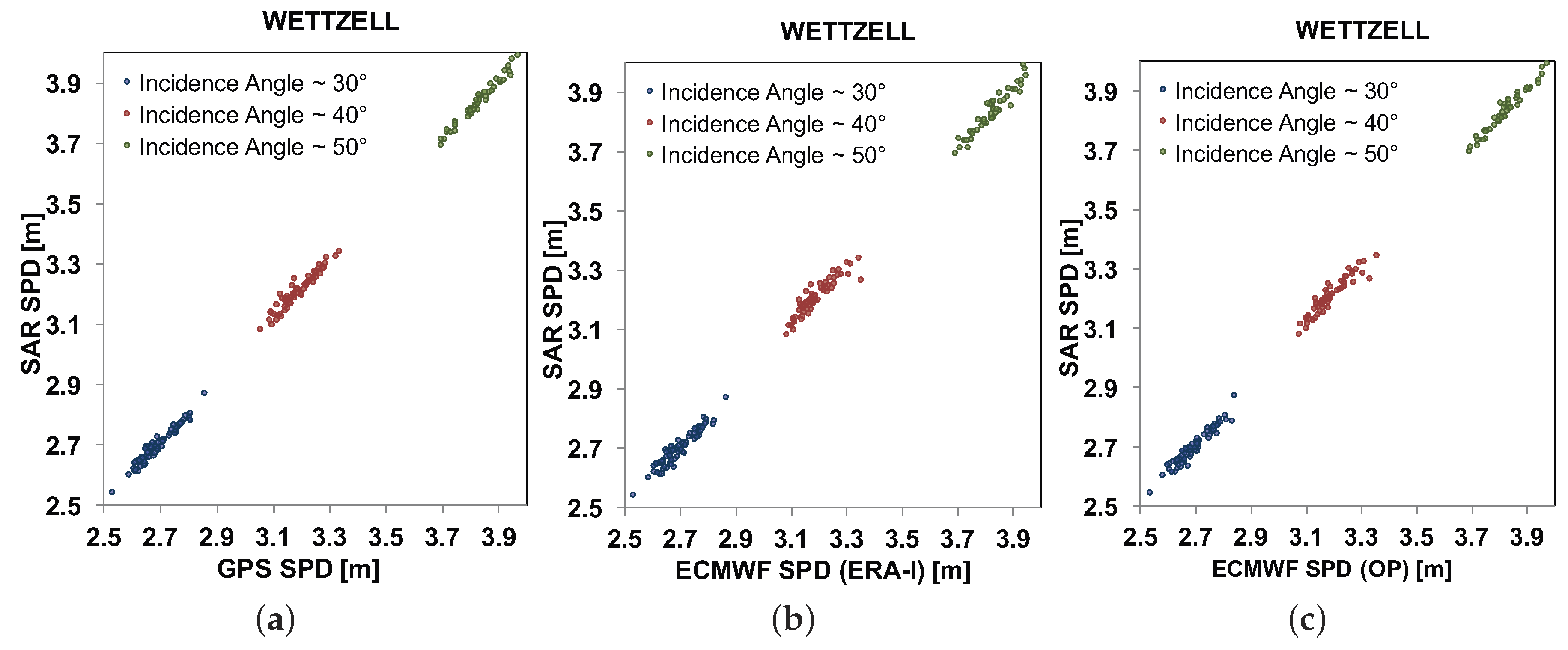
For this experiment, three trihedral CRs with m edge length were installed at two test sites close to permanent GNSS stations: two at the Wettzell geodetic observatory (WTZR) in Germany, with WTZR 01 orientated for ascending (ASC) orbits and WTZR 02 for descending (DSC) orbits, and one at the Metsähovi observatory in Finland (METS) for DSC orbits [42,43,44]. High resolution SAR images from the two German satellites TerraSAR-X (TSX-1) and TanDEM-X (TDX-1) have been acquired regularly: 176 scenes from July 2012 to October 2015 at WTZR and 155 scenes from December 2013 to February 2016 at METS. The acquisitions were acquired around 17:00 UTC at WTZR 01 and around 05:00 UTC at WTZR 02. At METS, SAR scenes were acquired around 05:00 UTC. ERA-Interim and OP data sets have been collected around the acquisition time, prepared according to the CR coordinate and integrated directly from the phase center of the CR to the upper limit of the ECMWF data in the direction towards the satellite position. In Figure 5, GPS SPD and ECMWF SPD show a clear agreement with SAR SPD with a correlation coefficient of in WTZR. Measurements are color coded according to the incidence angle class, i.e. the acquisition geometry. The impact of tropospheric delay increases in absolute value with increasing incidence angle.
Visually, GPS SPD has a better agreement with SAR SPD than the integrated delay based on ECMWF data sets (see Figure 5). We summarize the statistics of the comparison in Table 3 for each CR. Thanks to the higher temporal resolution (and to the fact that a GPS station is locally available), the best accuracy for the three CRs is achieved using GPS SPD as tropospheric delay corrections, with an accuracy that varies from to mm. The correction accuracy based on both ECMWF data sets are similar, having OP data a slightly better performance (around 1 mm) than ERA-Interim. The maximum mean offsets (up to mm) are observed in WTZR 01, which are mainly caused by the local ground subsidence that occurred after the installation of the CR [44].
4. Applications
The absolute accuracy of the tropospheric delay calculated with the direct integration method using ECMWF data has been validated against both GPS and CR measurements, demonstrating an accuracy in the centimeter range (Section 3). Note that the accuracy estimates also contain errors in the reference data used (GPS ZPD [38] and SAR SPD [1,44]).
In this section, we present several applications using the direct integration method to mitigate the tropospheric impact on SAR absolute range measurements (Section 4.1) and on SAR interferometry (Section 4.2).
4.1. Application to Absolute Ranging Measurements
In the framework of the DLR@Uni Munich Aerospace Project “Geodetic Earth Observation”, five CRs have been installed in three test sites [43,44]: two CRs at the geodetic observatory in Wettzell (WTZR) in Germany, two at GARS O’Higgins (OHIS) in the Antarctic Peninsula and one at Metsähovi (METS) in Finland. The two CRs in WTZR and the CR in METS have been used in Section 3.4 for ECMWF SPD validation purposes. From 2007 to 2014 over four hundreds of High Resolution SpotLight (HRSL) images have been acquired by both the TSX-1 and the TDX-1 satellites from ASC and DSC orbits. The acquisitions started firstly in July 2011 in WTZR, then in March 2013 in OHIS and finally in October 2013 in METS. Due to the near-polar orbit, most acquisitions are gathered in OHIS, where 10 different viewing geometries are available.
As discussed in Section 3.4, discrepancies between expected and measured absolute ranges are caused by geodetic and atmospheric effects [1,26,34]. Assuming that geodetic effects and ionospheric delay have been already compensated as described in [43,44], the remaining tropospheric delay can be compensated using either the IGS SPD (mapped ZPD) or the integrated ECMWF SPD using ERA-Interim data sets. A statistical analysis of the ranging residuals after these corrections has been performed. Only the data sets acquired before January 2015 have been evaluated. The results are reported in Table 4.
The mean values of the residuals are similar when using either IGS SPD or ECMWF SPD. However, the standard deviation varies from mm at WTZR (ASC) using IGS SPD to mm at OHIS (ASC) using ECMWF SPD. At WTZR, the difference of the standard deviation between IGS SPD and ECMWF SPD is more than 5 mm, namely mm for ASC and mm for DSC. At METS, the difference decreases to mm. Moreover, ECMWF SPD has a slightly better performance in OHIS ASC. These accuracy differences are mainly influenced by the different temperatures at each test site, which can be expressed as a function of latitude. For instance, test sites located at higher latitudes receive less sunlight than those at lower latitudes. Therefore, since the average temperature is lower at higher latitudes (e.g., METS and OHIS) the atmosphere can hold less water vapor, which leads to smaller water vapor variability and thus can be better modeled by NWP model (see Section 3.3.2) [16].
4.2. Application to Interferometric Measurements
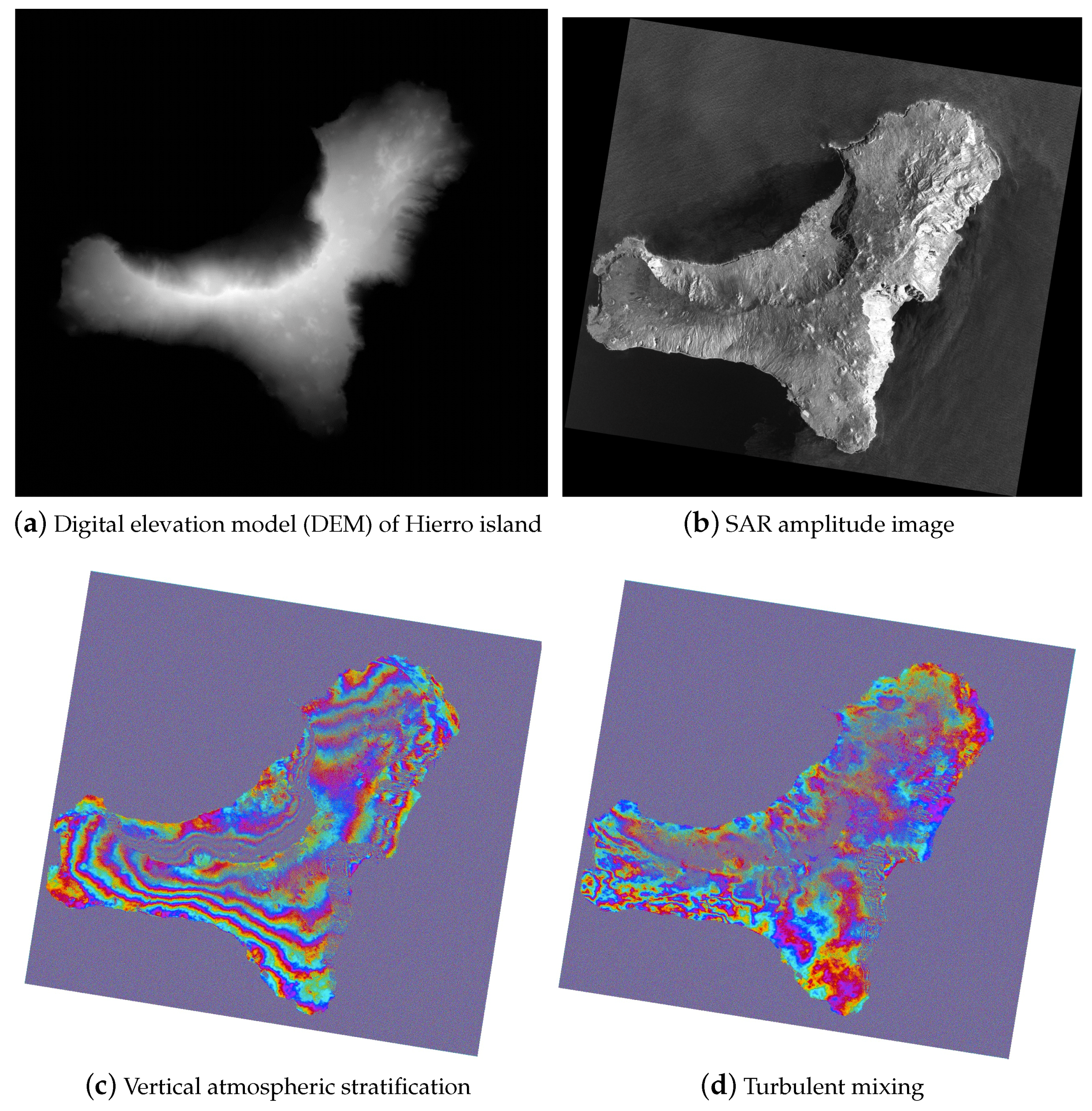
For SAR Interferometry (InSAR), the relative tropospheric delay between two acquisitions is of interest. According to its height dependency, the tropospheric delay can be divided into two parts: a height-dependent delay dominated by vertical stratification, the so-called stratified tropospheric delay, and a height-independent delay induced by turbulent mixing [6,17], which is described as a spatially correlated and temporally decorrelated effect. Let us illustrate these two delay components by means of interferograms of the Hierro Island in Spain. Firstly, in Figure 6c a height-dependent tropospheric delay can be clearly observed, which is solely due to different meteorological conditions. Secondly, the tropospheric delay effect induced by the turbulent atmosphere can be seen in Figure 6d, where in contrast to Figure 6c no correlation with height can be observed.
Two application test cases have been selected for interferometric applications. Firstly, the impact of tropospheric delay mitigation on persistent scatterer interferometry (PSI) estimation is demonstrated by using stacks of TerraSAR-X HRSL images of the Stromboli Volcano (Section 4.2.1). Secondly, an application to a stripe of Sentinel-1 interferograms in a mountainous area with a coverage of around km is presented (Section 4.2.2).
4.2.1. PSI Processing—Test Site: Stromboli Volcano, Italy
The Stromboli Volcano is one of the most active volcanoes. The Sciara del Fuoco (SdF) depression, the nested horseshoe-shaped scar opening located on the north-east flank, exhibits the most dynamic changes in Stromboli, which are caused by lava flows, rock falls, landslides, lava accumulation, condensation, etc. Current volcanic activities are concentrated within the summit crater zone, which is located in the upper part of the SdF. This summit crater zone has remained at its current position. Nevertheless, the number and size of vents located inside it are varying over time due to the changing magma level within the conduit. The two most recent major effusive eruptions, which occurred in 2002–2003 and in 2007, induced large morphological changes on the SdF.
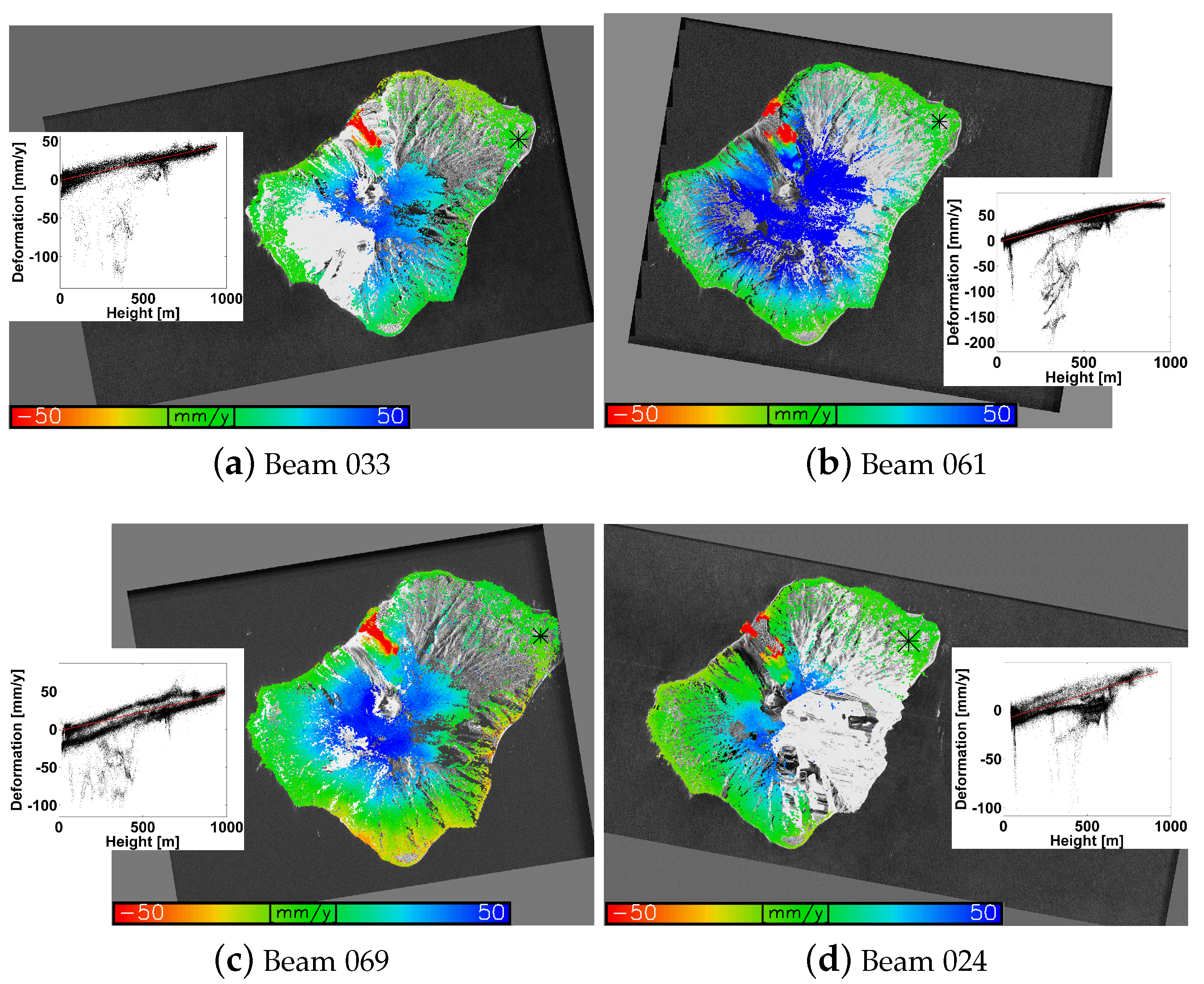
In the period from January to October 2008, 68 TerraSAR-X HRSL SAR images have been acquired from ascending and descending orbits with different incidence angles, which constitutes about 1 acquisition every days. The resulting four stacks have been processed using the PSI technique. For both ascending and descending geometries, on average around persistent scatterers (PSs) were detected per stack when selecting PSs with a signal-to-clutter ratio (SCR) larger than [45]. The final estimation results are presented in Figure 7, having selected as valid PSs those with an overall model test (OMT) smaller than [46]. A clear correlation between deformation estimates and height values is observed in the deformation maps as well as in the scatter plots depicted in Figure 7 [26].
At Stromboli the deformation and residual topography signals are overlaid with a strong stratified tropospheric delay in the differential interferometric phases. This is the cause for the height-correlated deformation signals that can be observed in Figure 7. Therefore it is necessary firstly to compensate the tropospheric delay and then to apply time series processing (PSI estimation) in order to reliably estimate deformation and residual topography.
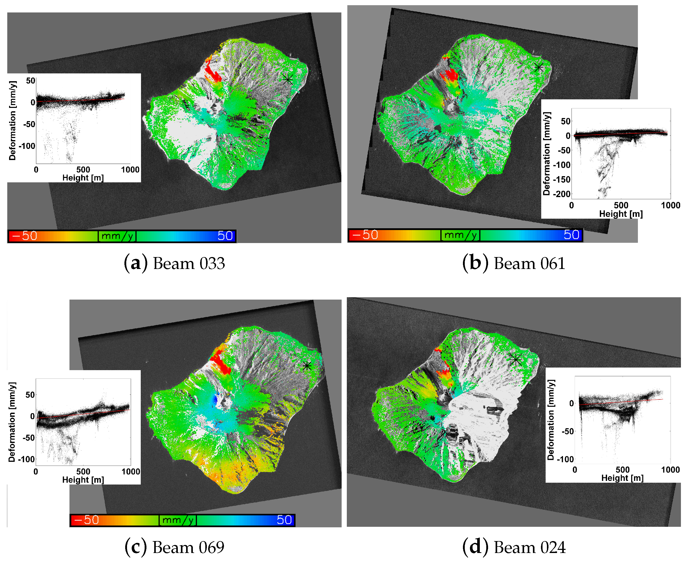
In order to mitigate the height-correlated stratified tropospheric delay, the differential tropospheric delay is firstly calculated for the PSs for each scene of the reference network using ERA-Interim data, then it is interpolated for all the other PSs and finally it is corrected on the differential interferometric phases. After this correction PSI processing is performed again. The resulting PS deformation maps after tropospheric delay mitigation are presented in Figure 8. In comparison to Figure 7, the height-dependent components have been effectively removed. Similar deformation patterns in SdF can be observed both in ascending and descending orbits. Some mismatches near craters are caused by horizontal deformation components, which are differently projected in the ascending and the descending geometries.
In order to assess the impact of the stratified tropospheric delay in the PSI estimates, the difference between the original estimates and the estimates after tropospheric delay compensation at identical PSs has been calculated. Note that an offset must be corrected for both difference of deformation estimates and difference of residual topography due to different reference points. Their maximum and minimum values as well as their correlation with height are summarized in Table 5. On the one hand, all deformation differences have a positive correlation (>85%) with height due to the temporal distribution (from January to October). The maximum relative deformation difference observed is mm/y in beam 061. On the other hand, differences of residual topography have both positive and negative correlation with height due to the different baseline distributions, exhibiting an absolute correlation higher than except for beam 033. The maximum relative residual topography difference observed is m in beam 069.
4.2.2. Wide Area Interferometry—Sentinel-1 Interferogram
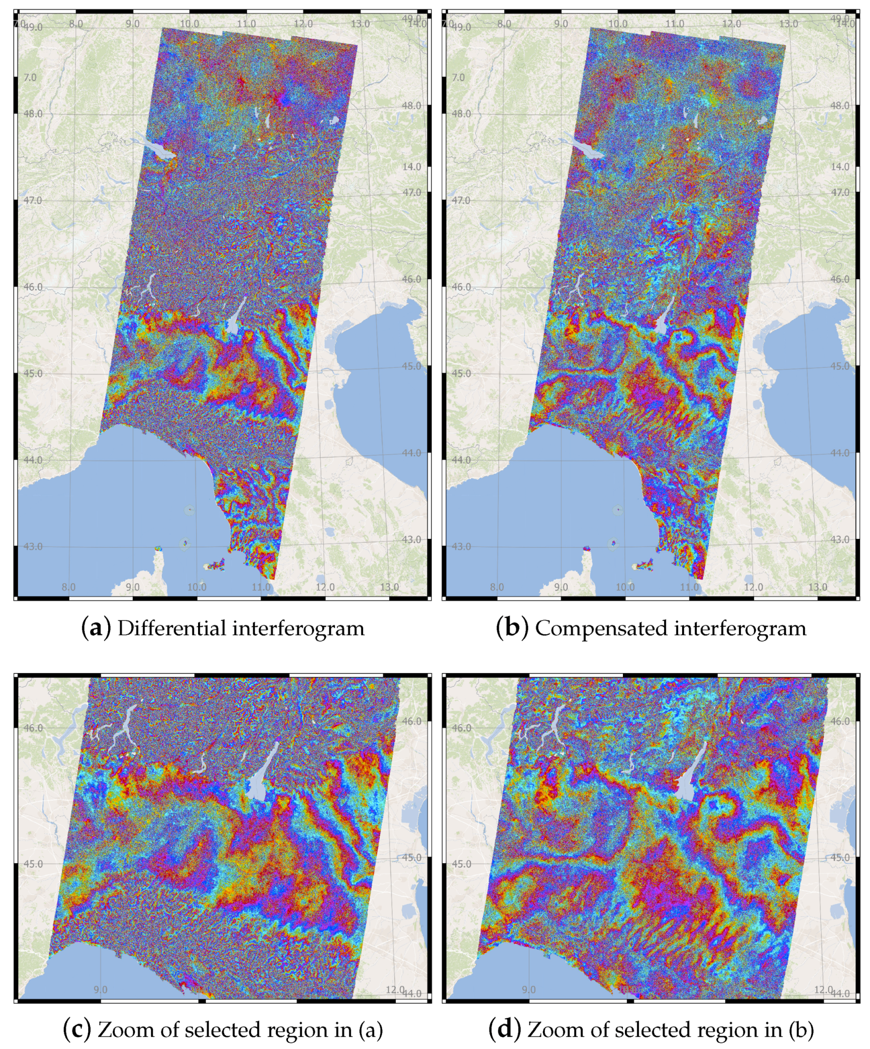
In this section, the OP-based integrated tropospheric delay as well as ionospheric delay (based on CODE TEC maps) and SET correction have been applied on four contiguous Sentinel-1 interferograms in order to demonstrate the application of integrated tropospheric delay in a large-scale. The Sentinel-1 images have been acquired by the Sentinel-1A satellite in the Interferometric Wide Swath Mode (IW) on 14 and 26 July 2016 at around 05:30 UTC. The resulting swath has a size of approximately 250 km by 750 km and spans from E to E in longitude and N to N in latitude. The effective baseline is around 21 m. In the acquired region the elevation varies from sea level up to almost 4000 m.
The interferograms have been processed using the Integrated Wide Area Processor (IWAP) [47,48] without and with compensation of atmospheric and geodetic delays. The results are shown in Figure 9. It can be clearly observed that the interferometric phase of the interferogram without corrections (see left column of Figure 9) is dominated by the differential stratified tropospheric delay. The tropospheric delay of the scenes varies from to m for the master acquisition and from to m for the slave acquisition. These big variations are due to the very big height variation within the scene as well as to the high incidence angle in far range. The maximum differential delay between the two acquisitions is of about 28 cm and the minimum of about 6 cm. After compensation of the tropospheric differential phases, the height-dependent phase has been significantly mitigated (see right column of Figure 9). Other atmospheric effects with lower magnitude are thus visible, such as the turbulent atmosphere, which is not contained in the ECMWF data but could be potentially modeled using meso-scale weather assimilation techniques [49,50].
5. Conclusions
The propagation of radar echoes across the troposphere (in fact, troposphere, stratosphere and mesosphere) causes a signal delay due to atmospheric refractivity. This delay has a mean value in the meter range and variations over time in the decimeter range. As a consequence, it has a great impact on both SAR absolute ranging measurements and differential interferometry. In this paper, we have shortly reviewed the modeling of the tropospheric delay for the direct integration method based on NWP products, focusing on the different refractivity models available and presenting our model choice. Its accuracy is evaluated using two NWP products provided by ECMWF: ERA-Interim and OP data. These products are provided at four analysis times per day (at 0, 6, 12 and 18 h UTC respectively) with a spatial resolution from approximately 80 km to less than 10 km. The accuracy of the integrated tropospheric delay using both products has been assessed using GPS ZPD of IGS stations and SAR SPD derived from TerraSAR-X HRSL CR measurements as reference.
In the zenith direction, the accuracy of the integrated tropospheric delay using ERA-Interim and OP is evaluated firstly against GPS ZPD at the Wettzell GNSS station. The standard deviation of the differences between the integrated ECMWF ZPD and GPS ZPD is about mm for ERA-Interim and mm for OP. Secondly, the validation of ERA-Interim products has been extended to a global scale using 268 permanent GNSS stations from the IGS network. The standard deviation of the difference between ECMWF ZPD and GPS ZPD varies from to mm. The accuracy of the integrated tropospheric delay at higher latitudes (>55) is better than mm, whereas that at lower latitudes (<30) is mostly between and mm. This variation of the accuracy is mainly correlated with the total water vapor content and depends on several factors such as location, station height and analysis time.
In the range direction, the accuracy of the integrated delay from both ECMWF data sets has been assessed using SAR SPD measurements as reference. More than 300 TerraSAR-X HRSL images of three CRs installed at the Wettzell geodetic observatory and at the Metsähovi observatory have been acquired. The standard deviation of the differences between ECMWF SPD and SAR SPD is approximately 15 mm for both ERA-Interim and OP, whereas their mean values vary from to mm.
Finally, the application of the direct integration method to tropospheric delay mitigation for SAR absolute range measurements and differential interferometry has been demonstrated. The impact on absolute range measurements has been evaluated using 5 CRs located at three far-distributed test sites. A ranging accuracy of to mm has been achieved. The accuracy using locally available GNSS station is better (from to mm). Nevertheless, using ECMWF data allows the exploitation of SAR absolute ranging with a centimeter-level accuracy without the requirement of a locally available GNSS station.
The impact of tropospheric delay mitigation on differential interferometry has been demonstrated for two test cases: TerraSAR-X PSI processing in the Stromboli Island and wide area Sentinel-1 differential interferometry. The differential interferograms without tropospheric delay correction exhibit a dominant phase component correlated with height which is caused by tropospheric stratification. This leads to height-dependent errors in the PSI estimates. The proposed direct integration method has been successfully applied in order to correct this stratified tropospheric phase component on the interferometric phase. As a result, the impact of the tropospheric delay on PSI estimation in the Stromboli test site has been effectively mitigated. The difference between PSI estimates without and with tropospheric delay mitigation is up to mm/year of relative deformation and up to m of relative residual topography. Due to the reduction of the height-dependent deformation component caused by the tropospheric delay it is now possible to observe the ground deformation patterns around the crater zones as well as to clearly delimitate the area with active deformation in the SdF. The mitigation of tropospheric stratification has been further demonstrated for wide area Sentinel-1 differential interferometry.
Author Contributions
X.C. conceived, designed and developed the techniques and experiments reported in this paper under supervision from M.E. X.C. carried out the experiments with inputs from the co-authors: U.B. provided the corner reflector SAR slant path delay measurements; F.R.G. performed the Sentinel-1 InSAR processing. X.C. wrote this paper.
Acknowledgments
The work was partially funded by the German Federal Ministry of Education and Research BMBF through its project “Exupéry: Managing Volcanic Unrest—The Volcano Fast Response System” and by the German Helmholtz Association through its DLR@Uni Alliance project “Munich Aerospace—High-resolution Geodetic Earth Observation: Correction Methods and Validation”.
Conflicts of Interest
The authors declare no conflict of interest.
Abbreviations
The following abbreviations are used in this manuscript:
| APL | Atmospheric pressure loading |
| ASC | Ascending |
| CD | Continental drift |
| CR | Corner reflector |
| DEM | Digital elevation model |
| DLR | German Aerospace Center |
| DSC | Descending |
| ECMWF | European Centre for Medium-Range Weather Forecasts |
| GNSS | Global navigation satellite system |
| GPS | Global positioning system |
| HRSL | High Resolution SpotLight |
| ID | Ionospheric delay |
| IFS | Integrated forecast system |
| IGS | International GNSS Service |
| InSAR | SAR interferometry |
| METS | CR test site in Metaähovi (Finland) |
| ML | Model level |
| NWP | Numerical weather prediction |
| OHIS | CR test site in GARS O’Higgins at the Antarctic Peninsula |
| OMT | Overall model test |
| OP | Operational data |
| OTL | Ocean tidal loading. |
| PSI | Persistent Scatterer (PS) interferometry |
| SAR | Synthetic aperture radar |
| SCR | Signal-to-Clutter Ratio |
| SET | Solid Earth tide |
| SPD | Slant range path delay |
| SWD | Slant range wet delay |
| TEC | Total electron content. |
| TDX-1 | German TanDEM-X satellite |
| TSX-1 | German TerraSAR-X satellite |
| WTZR | Wettzell GNSS station in EPN (Germany) |
| ZHD | Zenith hydrostatic delay |
| ZPD | Zenith path delay |
| ZWD | Zenith wet delay |
References
- Balss, U.; Cong, X.Y.; Brcic, R.; Rexer, M.; Minet, C.; Breit, H.; Fritz, T. High precision measurement on the absolute localization accuracy of TerraSAR-X. In Proceedings of the 2012 IEEE International Geoscience and Remote Sensing Symposium, Munich, Germany, 22–27 July 2012; pp. 1625–1628. [Google Scholar]
- Gisinger, C. Atmospheric Corrections for TerraSAR-X Derived from GNSS Observations. Master’s Thesis, Technische Universität München, Munich, Germany, 2012; pp. 1–117. [Google Scholar]
- Bamler, R.; Eineder, M. Split-band interferometry versus absolute ranging with wideband SAR systems. In Proceedings of the 2004 IEEE International Geoscience and Remote Sensing Symposium, Anchorage, AK, USA, 20–24 September 2004; pp. 980–984. [Google Scholar]
- Brcic, R.; Parizzi, A.; Eineder, M.; Bamler, R.; Meyer, F. Ionospheric effects in SAR interferometry: An analysis and comparison of methods for their estimation. In Proceedings of the 2011 IEEE International Geoscience and Remote Sensing Symposium, Vancouver, BC, Canada, 24–29 July 2011; pp. 1497–1500. [Google Scholar]
- Askne, J.; Nordius, H. Estimation of tropospheric delay for microwaves from surface weather data. Radio Sci. 1987, 22, 379–386. [Google Scholar] [CrossRef]
- Delacourt, C.; Briole, P.; Achache, J. Tropospheric corrections of SAR interferograms with strong topography application to Etna. Geophys. Res. Lett. 1998, 25, 2849–2852. [Google Scholar] [CrossRef]
- Li, Z.; Muller, J.-P.; Cross, P.; Fielding, E.J. Interferometric synthetic aperture radar (InSAR) atmospheric correction: GPS, Moderate Resolution Imaging Spectroradiometer (MODIS), and InSAR integration. J. Geophys. Res. Solid Earth 2005, 110, 2156–2202. [Google Scholar] [CrossRef]
- Cimini, D.; Pierdicca, N.; Pichelli, E.; Ferretti, R.; Mattioli, V.; Bonafoni, S.; Montopoli, M.; Perissin, D. On the accuracy of integrated water vapor observations and the potential for mitigating electromagnetic path delay error in InSAR. Atmos. Meas. Tech. Dis. 2012, 5, 1015–1030. [Google Scholar] [CrossRef] [Green Version]
- Jehle, M.; Perler, D.; Small, D.; Schubert, A.; Meier, E. Estimation of atmospheric path delays in TerraSAR-X data using models vs. measurements. Sensors 2008, 8, 8479–8491. [Google Scholar] [CrossRef] [PubMed] [Green Version]
- Cong, X.; Balss, U.; Eineder, M.; Fritz, T. Imaging Geodesy-Centimeter-level anging accuracy with TerraSAR-X: An update. IEEE Geosci. Remote Sens. Lett. 2012, 9, 948–952. [Google Scholar] [CrossRef]
- Nico, G.; Tomé, R.; Catalão, J.; Miranda, P.M.A. On the use of the WRF Model to mitigate tropospheric phase delay effects in SAR interferograms. IEEE Geosci. Remote Sens. Lett. 2011, 49, 948–952. [Google Scholar] [CrossRef]
- Catalão, J.; Nico, G.; Hanssen, R.F.; Catita, C. Merging GPS and atmospherically corrected InSAR data to map 3-D terrain displacement velocity. IEEE Geosci. Remote Sens. Lett. 2011, 49, 2354–2360. [Google Scholar] [CrossRef]
- Mateus, P.; Nico, G.; Tomé, R.; Catalão, J.; Miranda, P.M. Experimental study on the atmospheric delay based on GPS, SAR interferometry, and numerical weather model data. IEEE Geosci. Remote Sens. 2013, 51, 6–11. [Google Scholar] [CrossRef]
- Doin, M.-P.; Lasserre, C.; Peltzer, G.; Cavalié, O.; Doubre, C. Corrections of stratified tropospheric delays in SAR interferometry: Validation with global atmospheric models. J. Appl. Geophys. 2009, 69, 35–50. [Google Scholar] [CrossRef]
- Jolivet, R.; Agram, P.S.; Lin, N.Y.; Simons, M.; Doin, M.-P.; Peltzer, G.; Li, Z. Improving InSAR geodesy using global atmospheric models. J. Geophys. Res. Solid Earth 2014, 119, 2324–2341. [Google Scholar] [CrossRef]
- Wallace, J.M.; Hobbs, P.V. Atmospheric Science: An Introductory Survey; Elsevier Inc.: New York, NY, USA, 2006; 505p, ISBN 9780127329512. [Google Scholar]
- Hanssen, R.F. Radar Interferometry: Data Interpretation and Error Analysis; Springer: Berlin, Germany, 2001; ISBN 9780306476334. [Google Scholar]
- Smith, E.K.; Weintraubt, S. The constants in the equation for atmospheric refractive index at radio frequencies. Proc. IRE 1953, 41, 1035–1037. [Google Scholar] [CrossRef]
- Healy, S.B. Refractivity coefficients used in the assimilation of GPS radio occultation measurements. J. Geophys. Res. 2011, 116, 1–10. [Google Scholar] [CrossRef]
- Nafisi, V.; Urquhart, L.; Santos, M.C.; Nievinski, F.G.; Bohm, J.; Wijaya, D.D.; Zus, F. Comparison of ray-tracing packages for troposphere delays. IEEE Geosci. Remote Sens. 2012, 50, 469–481. [Google Scholar] [CrossRef]
- Saastamoinen, J. Atmospheric correction for the troposphere and stratosphere in radio ranging satellites. Geophys. Monogr. Ser. 1972, 15, 247–251. [Google Scholar]
- Thayer, G.D. An improved equation for the radio refractive index of air. Radio Sci. 1974, 9, 803–807. [Google Scholar] [CrossRef]
- Davis, J.L.; Herring, T.A.; Shapiro, I.I.; Rogers, A.E.E.; Elgered, G. Geodesy by radio interferometry: Effects of atmospheric modeling errors on estimates of baseline length. Radio Sci. 1985, 20, 1593–1607. [Google Scholar] [CrossRef] [Green Version]
- Bevis, M.; Businger, S.; Chiswell, S.; Herring, T.A.; Anthes, R.A.; Rocken, C.; Ware, R.H. An improved equation for the radio refractive index of air. J. Appl. Meteorol. 1994, 33, 379–386. [Google Scholar] [CrossRef]
- Rüeger, J.M. Refractive index formulae for radio waves. In Integration of Techniques and Corrections to Achieve Accurate Engineering. In Proceedings of the XXII FIG International Congress ACSM/SPRS Annual Conference, Washington, DC, USA, 19–26 April 2002; pp. 19–26. [Google Scholar]
- Cong, X. SAR Interferometry for Volcano Monitoring: 3D-PSI Analysis and Mitigation of Atmospheric Refractivity. Doctoral dissertation, Technische Universität München, Munich, Germany, 2014. [Google Scholar]
- Povic, J. ETA Model in Weather Forecast. Royal Institute of Technology, 2006. Available online: www.nada.kth.se/utbildning/grukth/exjobb/rapportlistor/2006/rapporter06/popovic_jelena_06054.pdf (accessed on 23 July 2018).
- Dee, D.P.; Uppala, S.M.; Simmons, A.J.; Berrisford, P.; Poli, P.; Kobayashi, S.; Andrae, U.; Balmaseda, M.A.; Balsamo, G.; Bauer, D.P.; et al. The ERA-Interim reanalysis: Configuration and performance of the data assimilation system. Q. J. R. Meteorol. Soc. 2011, 137, 553–597. [Google Scholar] [CrossRef]
- Hersbach, H.; Dee, D. ERA5 reanalysis is in production. ECMWF Newslett. 2016, 147, 7. [Google Scholar]
- Bock, O.; Keil, C.; Richard, E.; Flamant, C.; Bouin, M.-N. Validation of precipitable water from ECMWF model analyses with GPS and radiosonde data during the MAP SOP. Q. J. R. Meteorol. Soc. 2005, 131, 3013–3036. [Google Scholar] [CrossRef] [Green Version]
- Flentje, H.; Dörnbrack, A.; Fix, A.; Ehret, G.; Hólm, E. Evaluation of ECMWF water vapour fields by airborne differential absorption lidar measurements: A case study between Brazil and Europe. Atmos. Chem. Phys. 2007, 7, 5033–5042. [Google Scholar] [CrossRef]
- Schäfler, A.; Dörnbrack, A.; Kiemle, C.; Rahm, S.; Wirth, M. Tropospheric water vapor transport as determined from airborne Lidar measurements. J. Atmos. Ocean. Technol. 2010, 27, 2017–2030. [Google Scholar] [CrossRef]
- Schäfler, A.; Dörnbrack, A.; Wernli, H.; Kiemle, C.; Pfahl, S. Airborne lidar observations in the inflow region of a warm conveyor belt. Q. J. R. Meteorol. Soc. 2011, 137, 1257–1272. [Google Scholar] [CrossRef] [Green Version]
- Eineder, M.; Minet, C.; Steigenberger, P.; Cong, X.; Fritz, T. Imaging geodesy-Toward centimeter-level ranging accuracy with TerraSAR-X. IEEE Geosci. Remote Sens. 2011, 49, 661–671. [Google Scholar] [CrossRef]
- Dow, J.M.; Neilan, R.; Rizos, C. The international GNSS service in a changing landscape of global navigation satellite systems. J. Geod. 2009, 83, 191–198. [Google Scholar] [CrossRef]
- Bevis, M.; Businger, S.; Herring, T.A.; Rocken, C.; Anthes, R.A.; Ware, R.H. GPS meteorology: Remote sensing of atmospheric water vapor using the global positioning system. J. Geophys. Res. 1992, 97, 787–801. [Google Scholar] [CrossRef]
- Tregoning, P.; Boers, R.; O’Brien, D. Accuracy of absolute precipitable water vapor estimates from GPS observations. J. Geophys. Res. 1998, 103, 28701–28710. [Google Scholar] [CrossRef] [Green Version]
- Niell, A.E. Improved atmospheric mapping functions for VLBI and GPS. Earth Planets Sci. Lett. 2000, 52, 699–702. [Google Scholar] [CrossRef] [Green Version]
- Kacmarík, M.; Douša, J.; Dick, G.; Zus, F.; Brenot, H.; Möller, G.; Pottiaux, E.; Kapłon, J.; Hordyniec, P.; Václavovic, P.; et al. Inter-technique validation of tropospheric slant total delays. Atmos. Meas. Tech. 2017, 10, 2183–2208. [Google Scholar] [CrossRef] [Green Version]
- Böhm, J.; Möller, G.; Schindelegger, M.; Pain, G.; Weber, R. Development of an improved empirical model for slant delays in the troposphere (GPT2w). GPS Solut. 2005, 19, 433–441. [Google Scholar] [CrossRef]
- DGordon, N.D.; Jonko, A.K.; Forster, P.M.; Shell, K.M. An observationally based constraint on the water-vapor feedback. J. Geophs. Res. Atmos. 2013, 118, 12–435. [Google Scholar]
- Balss, U.; Breit, H.; Fritz, T.; Steinbrecher, U.; Gisinger, C.; Eineder, M. Analysis of internal timings and clock rates of TerraSAR-X. In Proceedings of the 2014 IEEE Geoscience and Remote Sensing Symposium, Quebec City, QC, Canada, 13–18 July 2014; pp. 2671–2674. [Google Scholar]
- Balss, U.; Gisinger, C.; Cong, X.Y.; Brcic, R.; Hackel, S.; Eineder, M. Precise Measurements on the Absolute Localization Accuracy of TerraSAR-X on the Base of Far-Distributed Test Sites. In Proceedings of the 10th European Conference on Synthetic Aperture Radar (EUSAR 2014), Berlin, Germany, 3–5 June 2014; pp. 993–996. [Google Scholar]
- Balss, U.; Gisinger, C.; Eineder, M. Measurements on the Absolute 2-D and 3-D Localization Accuracy of TerraSAR-X. Remote Sens. 2018, 10, 656. [Google Scholar] [CrossRef]
- Gernhardt, S.M. High Precision 3D Localization and Motion Analysis of Persistent Scatterers Using Meter-Resolution Radar Satellite Data. Doctoral dissertation, Technische Universität München, Munich, Germany, 2011. [Google Scholar]
- Kampes, B.M. Radar Interferometry: Persistent Scatterer Technique; Springer: Berlin, Germany, 2006. [Google Scholar]
- Rodriguze Gonzalez, F.; Adam, N.; Parizzi, A.; Brcic, R. The Integrated Wide Area Processor (IWAP): A processor for wide area persistent scatterer interferometry. ESA Liv. Planet Symp. 2013, 722, 353. [Google Scholar]
- Eineder, M.; Balss, U.; Suchandt, S.; Gisinger, C.; Cong, X.; Runge, H. A definition of next-generation SAR products for geodetic applications. In Proceedings of the 2015 IEEE International Geoscience and Remote Sensing Symposium (IGARSS), Milan, Italy, 26–31 July 2015; pp. 1638–1641. [Google Scholar]
- Pichelli, E.; Ferretti, R.; Cimini, D.; Panegrossi, G.; Perissin, D.; Pierdicca, N.; Rommen, B. InSAR water vapor data assimilation into mesoscale model MM5: Technique and pilot study. IEEE J. Sel. Top. Appl. Earth Obs. Remote Sens. 2015, 8, 3859–3875. [Google Scholar] [CrossRef]
- Mateus, P.; Miranda, P.M.A.; Nico, G.; Catalão, J.; Pinto, P.; Tomé, R. Assimilating InSAR maps of water vapor to improve heavy rainfall forecasts: A case study with two successive storms. J. Geophys. Res. 2018, 123, 1638–1641. [Google Scholar] [CrossRef]
Figure 1.
Sketch of validation methods. Types of delay measurements: (1) ZPD from GPS measurements () estimated at the GPS coordinates and projected with the local incidence angle (); (2) SPD from CR measurements () at the CR coordinates ; (3) integrated ECMWF delays: at and at . The integration steps are visualized as points over the integration path, with a smaller step under the effective height and a bigger step over until .

Figure 2.
Time-series analysis of integrated and approximated ZPD during 2015 at each analysis time (0, 6, 12 and 18 h UTC) compared to GPS ZPD at the Wettzell station. (a) Absolute ZPD: integrated using ERA-Interim (cyan) and OP (blue), empirical from GPT2w model (green) and GPS (black). (b) Difference between integrated and empirical ZPDs and GPS ZPD with same color coding.

Figure 3.
Global validation of ERA-Interim products from 2010 to 2015 based on 268 GPS stations of the IGS network: (a) mean value of the integrated ZPD; (b) standard deviation of the difference between the integrated ZPD and GPS ZPD.
Figure 3.
Global validation of ERA-Interim products from 2010 to 2015 based on 268 GPS stations of the IGS network: (a) mean value of the integrated ZPD; (b) standard deviation of the difference between the integrated ZPD and GPS ZPD.

Figure 4.
Dependency on absolute latitude of mean ERA-Interim ZPD and standard deviation of ZPD residuals with respect to GPS ZPD evaluated at IGS stations. (Left) Mean integrated ZPD as a function of absolute latitude. (Right) Standard deviation of the difference between integrated and GPS ZPD as a function of absolute latitude. The color coding is used to indicate the height of the IGS stations.

Figure 5.
Correlation analysis of absolute localization residuals of both CRs in WTZR: (a) scatter plot of the mapped range delay based on GPS ZPD (GPS SPD) and the SAR range residuals (SAR SPD). (b) scatter plot of the range delays integrated using ERA-Interim data (ECMWF SPD) and SAR SPD. (c) scatter plot of the range delays integrated using OP data (ECMWF SPD) and SAR SPD. Each dot represents a SAR acquisition, which is color coded according to the different incidence angle classes: ∼ in blue; ∼ in red and ∼ in green.

Figure 6.
Tropospheric propagation delay effects on SAR interferometry due to vertical stratification and turbulent mixing: an example in the Hierro Island (Spain) using TerraSAR-X StripMap images. (a) Digital elevation model (DEM) of Hierro Island, with elevation varying from sea level (black) to about 1542 m (white). (b) SAR intensity image acquired on 10 October 2011. (c) Differential interferogram with master image acquired on 10 October 2011 and slave image on 21 October 2011 with an effective baseline of about 58 m. (d) Differential interferogram with master image acquired on 4 December 2011 and slave image on 15 December 2011 with an effective baseline of about 80 m. In (c) the interferometric phase is dominated by vertical stratification, whereas in (d) by turbulent mixing. Note that both are 11-day repeat pass interferograms.

Figure 7.
PS deformation maps without tropospheric correction of four TerraSAR-X HRSL stacks over the Stromboli Island with the geocoded average amplitude image as background. These stacks cover the time period January to October 2008 and contain (a) 18, (b) 17, (c) 16 and (d) 17 acquisitions. A scatter plot of deformation versus height is also illustrated for each of them. A linear fit is presented as a red line on each scatter plot. A clear correlation between deformation estimates and height is observed.

Figure 8.
PS deformation maps after mitigation of the differential tropospheric delay for the stacks introduced in Figure 7. A comparison with Figure 7 clearly shows that the compensation of ECMWF based integrated tropospheric differential delay corrections has effectively mitigated the impact of tropospheric stratification.

Figure 9.
Eight Sentinel-1 images acquired in Interferometric Wide Swath Mode (IW) on 14 and 26 July 2016 at around 05:30 UTC. (a) Differential interferogram. (b) Atmospheric delays (tropospheric and ionospheric) and SET compensated interferogram. Zooms of the selected region around Po Valley provided in (c,d). Contains modified Copernicus Sentinel data 2016. Background: Data © OpenStreetMap contributors, Rendering © DLR/EOC.


Table 1.
Summary of the coefficient constants , and from [18,19,21,22,23,24,25]. They are divided into three groups: (1) ideal gases; (2) non-ideal gases; (3) non-ideal gases based on an approximated equation. Differences relative to the reference ZPD ( with rounded coefficient constants [18]) are calculated for NWP products during August 2013 at the Wettzell GNSS station. The mean value and the standard deviation of the differences are presented.
| Authors (Year) | (K/hPa) | (K/hPa) | (K/ hPa) | ZPD Diff. (mm) | |
|---|---|---|---|---|---|
| Mean | Std | ||||
| Ideal Gas | |||||
| Smith and Weintraubt [18] | |||||
| Saastamoinen [21] | |||||
| Rüeger [25] (best available) | <0.1 | ||||
| Rüeger [25] (best average) | <0.1 | ||||
| Healy [19] | <0.1 | ||||
| Non-ideal Gases | |||||
| Thayer [22] | |||||
| Davis et al. [23] | |||||
| Healy [19] | |||||
| Non-ideal Gases—Approximated Equation | |||||
| Bevis et al. [24] | |||||
Table 2.
Summary of ECMWF reanalysis data sets (ERA-Interim and ERA5) and OP specifications: horizontal resolution in latitude/longitude; vertical resolution model level (ML); IFS release cycle and date [28]. Only releases with major changes, either in spatial resolution or ML, are reported.
Table 2.
Summary of ECMWF reanalysis data sets (ERA-Interim and ERA5) and OP specifications: horizontal resolution in latitude/longitude; vertical resolution model level (ML); IFS release cycle and date [28]. Only releases with major changes, either in spatial resolution or ML, are reported.
| ECMWF Products | Horizontal Resolution (deg) | Vertical Resolution | IFS Release | Release Date |
|---|---|---|---|---|
| Operational | 0.100 | 137-Level | Cycle 41r2 | 8 March 2016 |
| 0.125 | 137-Level | Cycle 38r2 | 26 June 2013 | |
| 0.125 | 91-Level | Cycle 38r1 | 11 March 2008 | |
| 0.225 | 91-Level | Cycle 30r1 | 1 February 2006 | |
| 0.350 | 60-Level | Cycle 23r3 | 21 November 2000 | |
| ERA-Interim | 0.750 | 60-Level | Cycle 31r2 | 1 January 2006 |
| ERA5 | 0.280 | 137-Level | Cycle 41r2 | 1 January 2018 |
Table 3.
Validation results using SAR SPDs as reference.
| CR ID | Input Data | Mean (mm) | STD (mm) |
|---|---|---|---|
| WTZR 01 (ASC) | GPS ZPD | ||
| ERA-Interim | |||
| Operational | |||
| WTZR 02 (DSC) | GPS ZPD | ||
| ERA-Interim | |||
| Operational | |||
| METS (DSC) | GPS ZPD | ||
| ERA-Interim | |||
| Operational |
Table 4.
Statistical analysis of absolute range residuals using IGS SPD (mapped ZPD) and integrated ECMWF SPD at test sites: Wettzell (WTZR) in Germany, GARS O’Higgins (OHIS) at the Antarctic Peninsula and Metsähovi (METS) in Finland.
Table 4.
Statistical analysis of absolute range residuals using IGS SPD (mapped ZPD) and integrated ECMWF SPD at test sites: Wettzell (WTZR) in Germany, GARS O’Higgins (OHIS) at the Antarctic Peninsula and Metsähovi (METS) in Finland.
| Test Site Code | Crossing Orbit Direction | IGS SPD | ECMWF SPD | ||
|---|---|---|---|---|---|
| Mean (mm) | STD (mm) | Mean (mm) | STD [mm] | ||
| WTZR | ASC | ||||
| DSC | |||||
| OHIS | ASC | ||||
| DSC | |||||
| METS | DSC | ||||
Table 5.
Summary of statistical analysis of the differences of two PSI processing results without and with tropospheric delay correction: maximum and minimum value of deformation differences and residual topography differences as well as their correlation with height. An offset compensation has been performed on both differences in order to account for the different reference points.
| Beam | (mm/year) | (m) | ||||
|---|---|---|---|---|---|---|
| Nr. | Max | Min | Corr. (-) | Max | Min | Corr. (-) |
| 033 | ||||||
| 061 | ||||||
| 069 | ||||||
| 024 | ||||||
© 2018 by the authors. Licensee MDPI, Basel, Switzerland. This article is an open access article distributed under the terms and conditions of the Creative Commons Attribution (CC BY) license (http://creativecommons.org/licenses/by/4.0/).
Share and Cite
MDPI and ACS Style
Cong, X.; Balss, U.; Rodriguez Gonzalez, F.; Eineder, M. Mitigation of Tropospheric Delay in SAR and InSAR Using NWP Data: Its Validation and Application Examples. Remote Sens. 2018, 10, 1515. https://doi.org/10.3390/rs10101515
AMA Style
Cong X, Balss U, Rodriguez Gonzalez F, Eineder M. Mitigation of Tropospheric Delay in SAR and InSAR Using NWP Data: Its Validation and Application Examples. Remote Sensing. 2018; 10(10):1515. https://doi.org/10.3390/rs10101515
Chicago/Turabian StyleCong, Xiaoying, Ulrich Balss, Fernando Rodriguez Gonzalez, and Michael Eineder. 2018. "Mitigation of Tropospheric Delay in SAR and InSAR Using NWP Data: Its Validation and Application Examples" Remote Sensing 10, no. 10: 1515. https://doi.org/10.3390/rs10101515
Note that from the first issue of 2016, this journal uses article numbers instead of page numbers. See further details here.