A Novel Change Detection Approach for Multi-Temporal High-Resolution Remote Sensing Images Based on Rotation Forest and Coarse-to-Fine Uncertainty Analyses


Abstract
:
1. Introduction
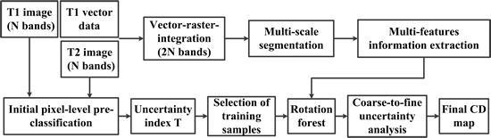
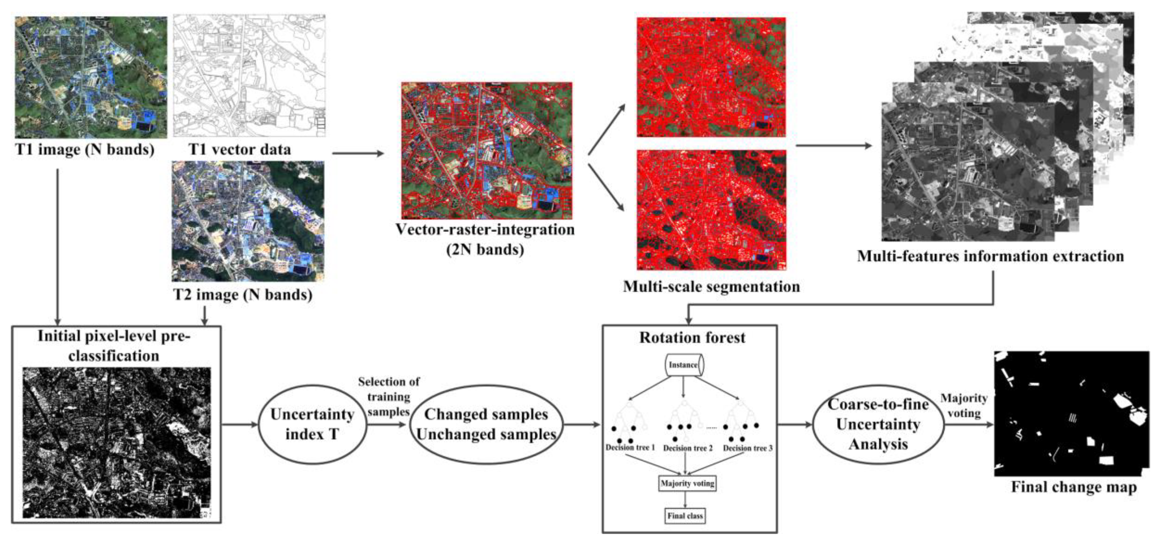
2. Methodology
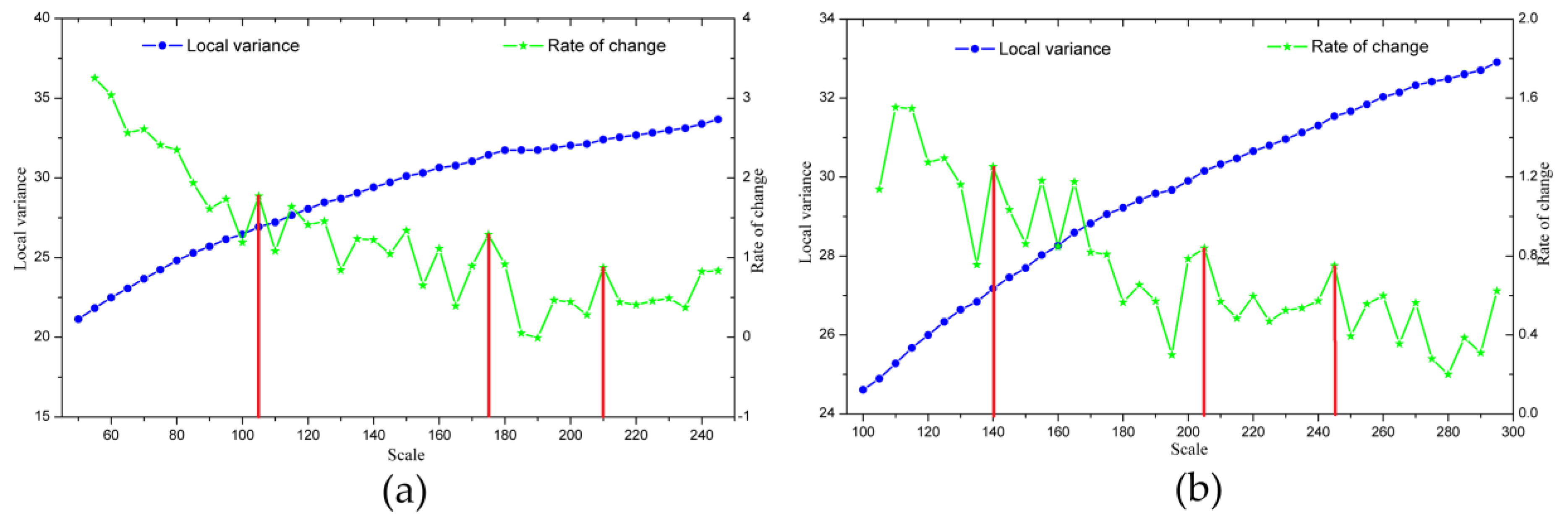
2.1. MTIS and Estimation of Scale Parameters
2.2. Selection of Training Samples
2.3. Multi-Feature Information Extraction
2.4. OBCD Based on RoF and Coarse-to-Fine Uncertainty Analyses
3. Experiments and Results
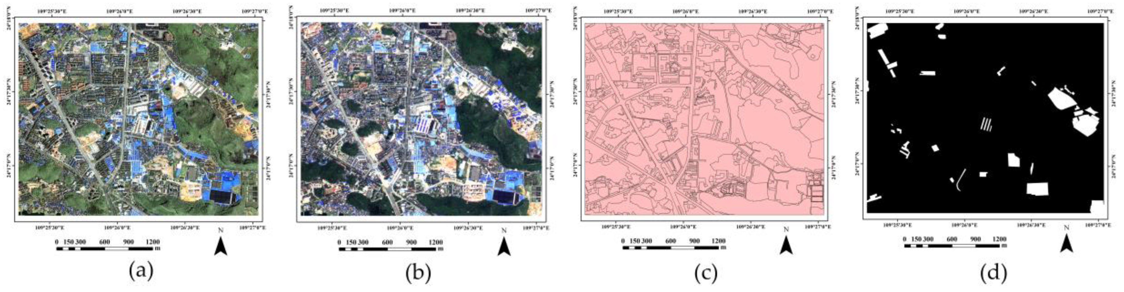
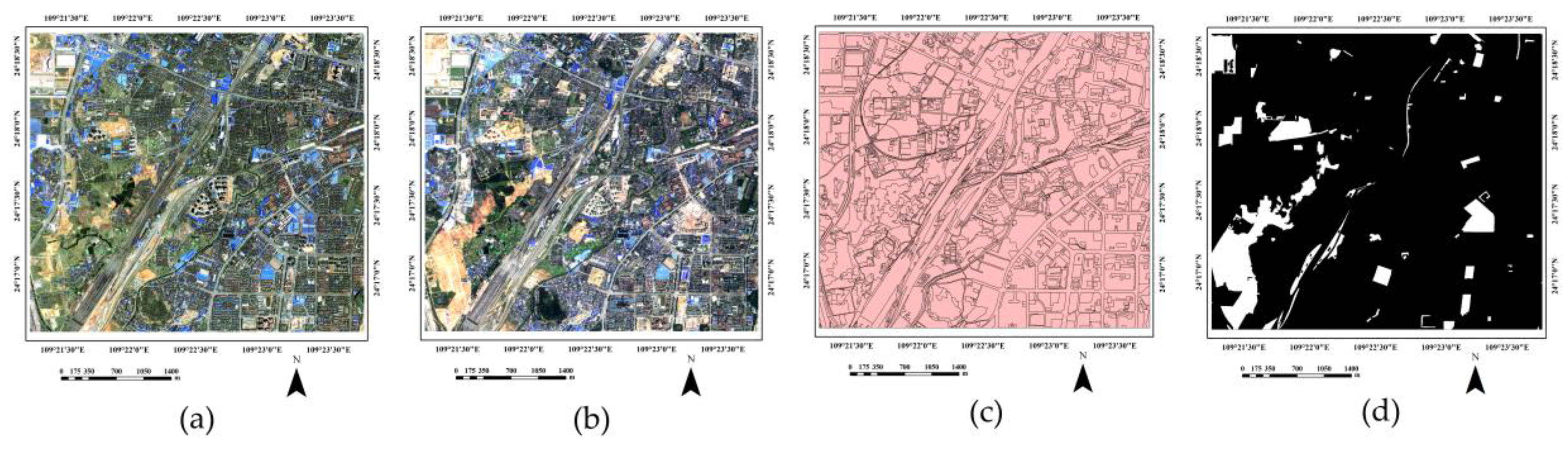
3.1. Dataset Description
3.2. Evaluation Metrics
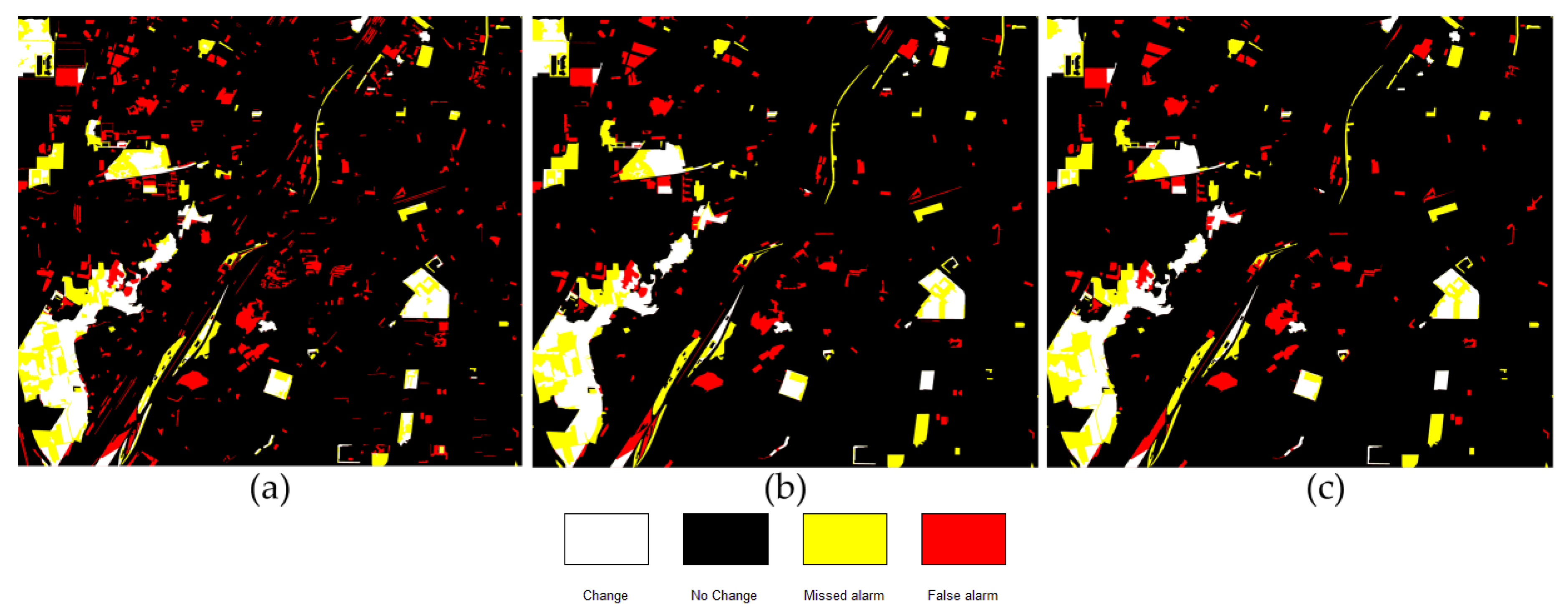
- False alarms (FA): The number of unchanged pixels that are incorrectly detected as having changed, ; the false alarm rate is defined as , where is the total number of unchanged pixels.
- Missed alarms (MA): The number of changed pixels that are incorrectly detected as being unchanged, ; the missed alarm rate is defined as , where is the total number of changed pixels.
- Overall error (OE): The total errors caused by FA and MA; the overall alarm rate is calculated as .
- Kappa: The Kappa coefficient is a statistical measure of accuracy or agreement, which reflects the consistency between experimental results and ground truth data, and is expressed as , where indicates the true consistency and indicates the theoretical consistency.
3.3. Experimental Results and Analysis
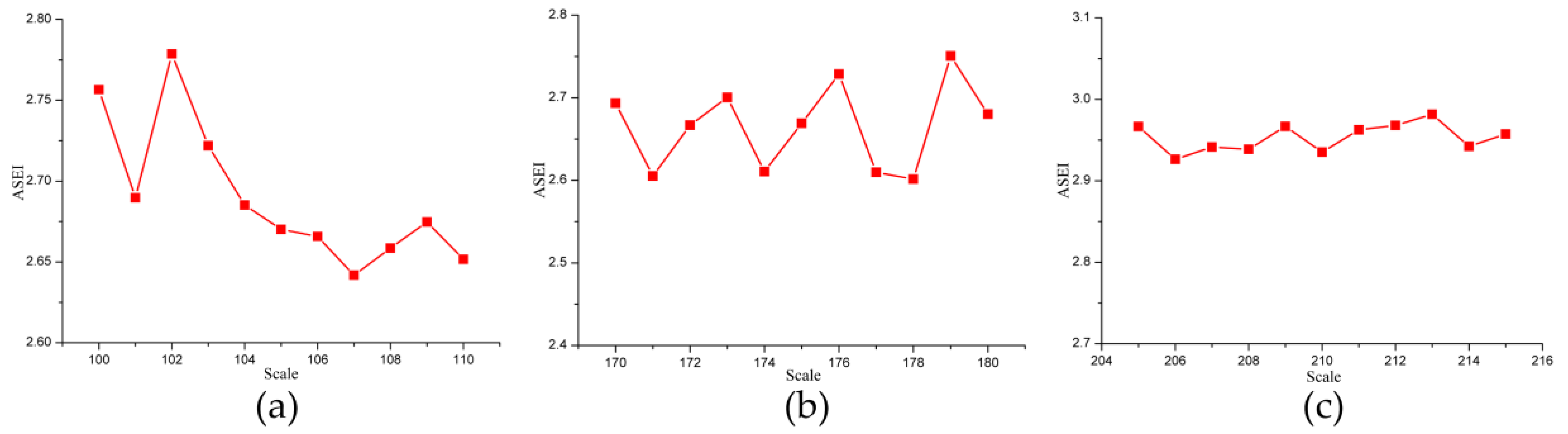
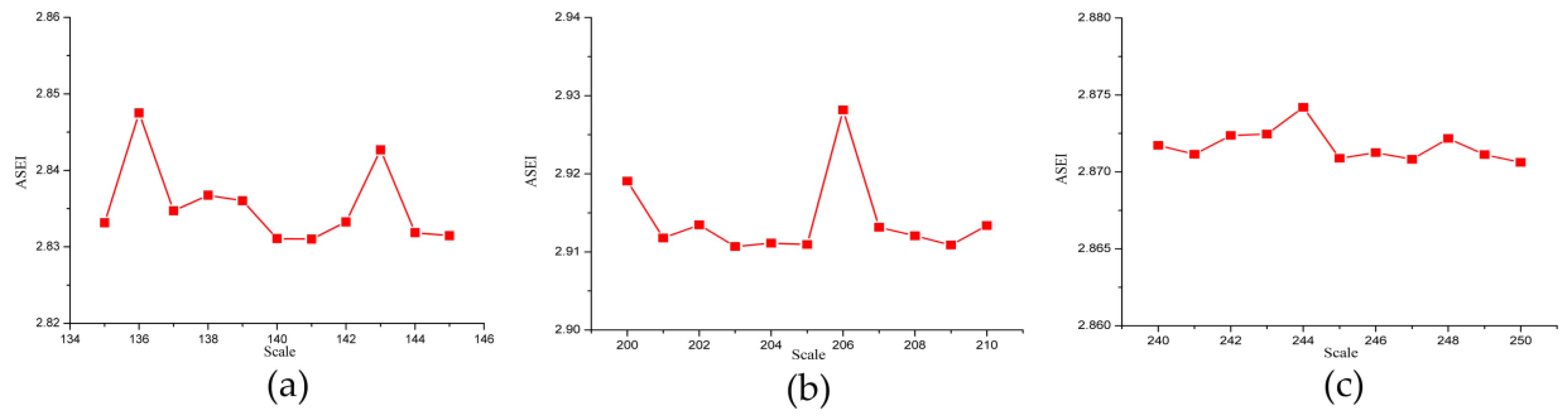
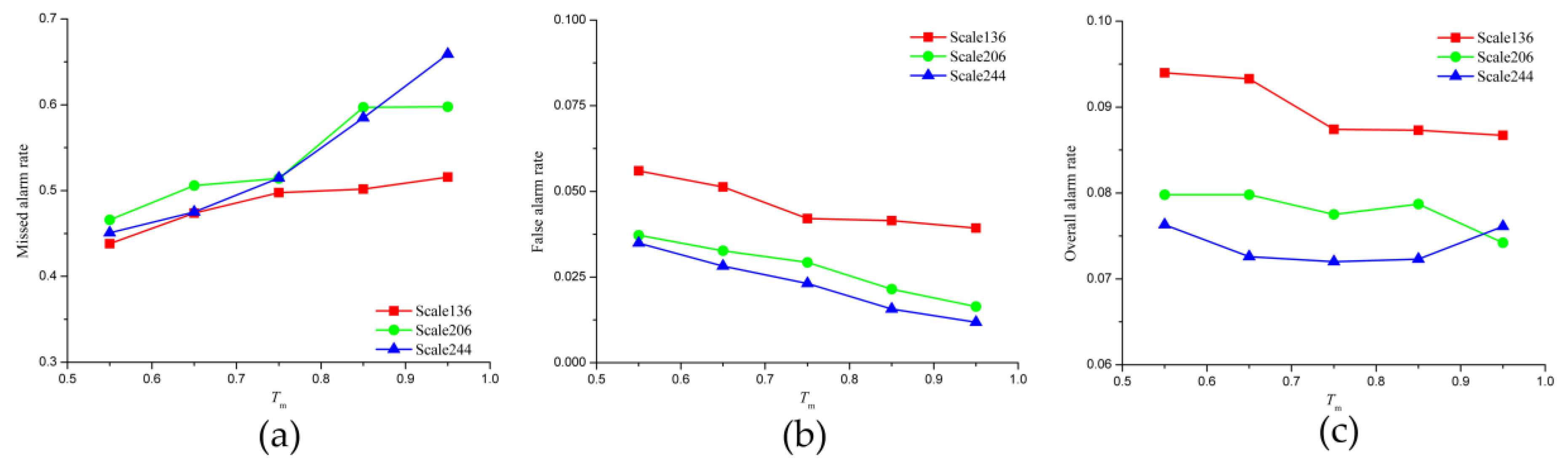
3.3.1. Test of Scale Parameters
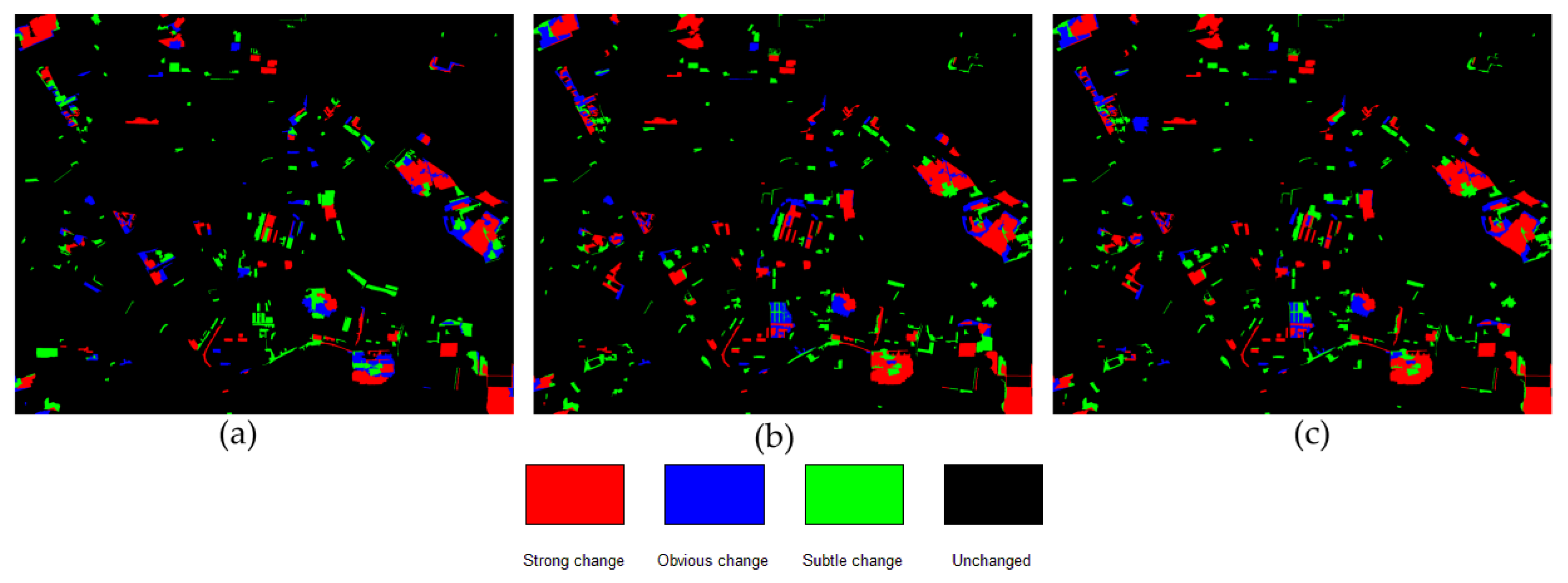
3.3.2. Results for DS1
3.3.3. Results for DS2
4. Discussion
5. Conclusions and Perspective
Author Contributions
Acknowledgments
Conflicts of Interest
Abbreviations
| CD | Change detection |
| OBCD | Object-based change detection |
| PBCD | Pixel-based change detection |
| NCIA | Neighbourhood correlation image analysis |
| HVM | Historical land use vector map |
| RoF | Rotation forest |
| RF | Random forest |
| ELM | Extreme learning machine |
| IR-MAD | Iteratively reweighted multivariate alteration detection |
| MV | Majority voting |
| MRF | Markov random field |
| CRF | Conditional Random Field |
| OCVA | Object-based change vector analysis |
| OCC | Object-based correlation coefficient |
| OCST | Object-based chi-square (χ2) transformation |
| GIS | Geographic information system |
| MTIS | Multi-temporal image segmentation |
| MRS | Multi-resolution segmentation |
| STS | Single-temporal segmentation (STS) |
| MTSS | Multi-temporal separate segmentation |
| MTCS | Multi-temporal combined segmentation |
| ESP | Estimation of scale parameter |
| SEI | Segmentation evaluation index |
| ASEI | Average segmentation evaluation index |
| LV | Local variance |
| ROC-LV | Rates of change of LV |
| GLCM | Gray-level co-occurrence matrix |
| PCA | Principal component analysis |
| FA | False alarms |
| MA | Missed alarms |
| OE | Overall error |
References
- Hussain, M.; Chen, D.; Cheng, A.; Wei, H.; Stanley, D. Change detection from remotely sensed images: From pixel-based to object-based approaches. ISPRS J. Photogramm. Remote Sens. 2013, 80, 91–106. [Google Scholar] [CrossRef]
- Bovolo, F.; Bruzzone, L. A theoretical framework for unsupervised change detection based on change vector analysis in the polar domain. IEEE Trans. Geosci. Remote Sens. 2007, 45, 218–236. [Google Scholar] [CrossRef]
- Hao, M.; Shi, W.; Zhang, H.; Li, C. Unsupervised change detection with expectation-maximization-based level set. IEEE Geosci. Remote Sens. Lett. 2013, 11, 210–214. [Google Scholar] [CrossRef]
- Cao, G.; Liu, Y.; Shang, Y. Automatic change detection in remote sensing images using level set method with neighborhood constraints. J. Appl. Remote Sens. 2014, 8. [Google Scholar] [CrossRef]
- Bruzzone, L.; Prieto, D. Automatic analysis of the difference image for unsupervised change detection. IEEE Trans. Geosci. Remote Sens. 2000, 38, 1171–1182. [Google Scholar] [CrossRef]
- Hao, M.; Zhang, H.; Shi, W.; Deng, K. Unsupervised change detection using fuzzy -means and MRF from remotely sensed images. Remote Sens. Lett. 2013, 4, 1185–1194. [Google Scholar] [CrossRef]
- Zhou, L.; Cao, G.; Li, Y.; Shang, Y. Change detection based on conditional random field with region connection constraints in high-resolution remote sensing images. IEEE J. Sel. Top. Appl. Earth Observ. Remote Sens. 2016, 9, 3478–3488. [Google Scholar] [CrossRef]
- Cao, G.; Zhou, L.; Li, Y. A new change-detection method in high-resolution remote sensing images based on a conditional random field model. Int. J. Remote Sens. 2016, 37, 1173–1189. [Google Scholar] [CrossRef]
- Nielsen, A. The regularized iteratively reweighted mad method for change detection in multi- and hyper-spectral data. IEEE Trans. Image Process. 2007, 16, 463–478. [Google Scholar] [CrossRef] [PubMed]
- Celik, T. Unsupervised change detection in satellite images using principal component analysis and k-means clustering. IEEE Geosci. Remote Sens. Lett. 2009, 6, 772–776. [Google Scholar] [CrossRef]
- Hazel, G. Object-level change detection in spectral imagery. IEEE Trans. Geosci. Remote Sens. 2001, 39, 553–561. [Google Scholar] [CrossRef]
- Wang, W.J.; Zhao, Z.M.; Zhu, H.Q. Object-oriented Change Detection Method Based on Multi-scale and Multi-Feature Fusion. In Proceedings of the 2009 Urban Remote Sensing Joint Event, Shanghai, China, 20–22 May 2009; pp. 1–5. [Google Scholar]
- Emary, E.M.; El-Saied, K.M.; Onsi, H.M. A proposed multi-scale approach with automatic scale selection for image change detection. Egypt. J. Remote Sens. Space Sci. 2010, 13, 1–10. [Google Scholar] [CrossRef]
- Wang, C.; Xu, M.X.; Wang, X.; Zheng, S.; Ma, Z. Object-oriented change detection approach for high-resolution remote sensing images based on multi-scale fusion. J. Appl. Remote Sens. 2013, 7. [Google Scholar] [CrossRef]
- Hao, M.; Shi, W.; Zhang, H.; Wang, Q.; Deng, K. A scale-driven change detection method incorporating uncertainty analysis for remote sensing images. Remote Sens. 2016, 8. [Google Scholar] [CrossRef]
- Xiao, P.; Zhang, X.; Wang, D. Change detection of built-up land: A framework of combining pixel-based detection and object-based recognition. ISPRS J. Photogramm. Remote Sens. 2016, 119, 402–414. [Google Scholar] [CrossRef]
- Xiao, P.; Yuan, M.; Zhang, X.; Feng, X.; Guo, Y. Cosegmentation for object-based building change detection from high-resolution remotely sensed images. IEEE Trans. Geosci. Remote Sens. 2017, 55, 1587–1603. [Google Scholar] [CrossRef]
- Sun, K.; Chen, Y. The Application of objects change vector analysis in object-level change detection. In Proceedings of the International Conference on Computational Intelligence and Industrial Application (PACIIA), Wuhan, China, 6–7 November 2010; Volume 15, pp. 383–389. [Google Scholar]
- Wang, L.; Yan, L.I.; Wang, Y. Research on land use change detection based on an object-oriented change vector analysis method. Geogr. Res. 2014, 27, 74–80. [Google Scholar]
- Wang, Y.; Shu, N.; Gong, Y. A study of land use change detection based on high resolution remote sensing images. Remote Sens. Land Resour. 2012, 24, 43–47. [Google Scholar]
- Chen, Q.; Chen, Y. Multi-Feature Object-Based Change Detection Using Self-Adaptive Weight Change Vector Analysis. Remote Sens. 2016, 8. [Google Scholar] [CrossRef]
- Vázquezjiménez, R. Applying the chi-square transformation and automatic secant thresholding to Landsat imagery as unsupervised change detection methods. J. Appl. Remote Sens. 2017, 11. [Google Scholar] [CrossRef]
- Chen, J.; Xia, J.; Du, P.; Chanussot, J. Combining Rotation Forest and Multi-scale Segmentation for the Classification of Hyper-spectral Data. IEEE J. Sel. Top. Appl. Earth Observ. Remote Sens. 2016, 9, 4060–4072. [Google Scholar] [CrossRef]
- Gang, C.; Geoffrey, J.; Luis, M.; Michael, A. Object-based change detection. Int. J. Remote Sens. 2012, 33, 4434–4457. [Google Scholar]
- Zhang, Y.; Peng, D.; Huang, X. Object-Based Change Detection for VHR Images Based on Multiscale Uncertainty Analysis. IEEE Geosci. Remote Sens. Lett. 2018, 15, 13–17. [Google Scholar] [CrossRef]
- Alboody, A.; Sedes, F.; Inglada, J. Post-classification and spatial reasoning: New approach to change detection for updating GIS database. In Proceedings of the IEEE International Conference on Information and Communication Technologies: From Theory To Applications, Damascus, Syria, 7–11 April 2008; pp. 1–7. [Google Scholar]
- Yu, C.; Shen, S.; Huang, J.; Yi, Y. An object-based change detection approach using high-resolution remote sensing image and GIS data. In Proceedings of the IEEE International Conference on Image Analysis and Signal Processing, Zhejiang, China, 9–11 April 2010; pp. 565–569. [Google Scholar]
- Hanif, M.; Mustafa, M.; Hashim, A.; Yusof, K. Spatio-temporal change analysis of Perak river basin using remote sensing and GIS. In Proceedings of the IEEE International Conference on Space Science and Communication, Langkawi, Malaysia, 10–12 August 2015; pp. 225–230. [Google Scholar]
- Sofina, N.; Ehlers, M. Building Change Detection Using High Resolution Remotely Sensed Data and GIS. IEEE J. Sel. Top. Appl. Earth Observ. Remote Sens. 2017, 9, 3430–3438. [Google Scholar] [CrossRef]
- Ayele, G.T.; Tebeje, A.K.; Demissie, S.S.; Belete, M.A.; Jemberrie, M.A.; Teshome, W.M.; Mengistu, D.T.; Teshale, E.Z. Time Series Land Cover Mapping and Change Detection Analysis Using Geographic Information System and Remote Sensing, Northern Ethiopia. Air Soil Water Res. 2018, 11. [Google Scholar] [CrossRef]
- Dewan, A.; Yamaguchi, Y. Land use and land cover change in Greater Dhaka, Bangladesh: Using remote sensing to promote sustainable urbanization. Appl. Geogr. 2009, 29, 390–401. [Google Scholar] [CrossRef]
- Wu, C.; Du, B.; Cui, X.; Zhang, L. A post-classification change detection method based on iterative slow feature analysis and Bayesian soft fusion. Remote Sens. Environ. 2017, 199, 241–255. [Google Scholar] [CrossRef]
- Aguirre, J.; Seijmonsbergen, A.; Duivenvoorden, J. Optimizing land cover classification accuracy for change detection, a combined pixel-based and object-based approach in a mountainous area in Mexico. Appl. Geogr. 2012, 34, 29–37. [Google Scholar] [CrossRef] [Green Version]
- Lu, J.; Li, J.; Chen, G.; Zhao, L.; Xiong, B.; Kuang, G. Improving Pixel-Based Change Detection Accuracy Using an Object-Based Approach in Multi-temporal SAR Flood Images. IEEE J. Sel. Top. Appl. Earth Observ. Remote Sens. 2015, 8, 3486–3496. [Google Scholar] [CrossRef]
- Feng, W.; Sui, H.; Tu, J.; Huang, W.; Sun, K. Remote Sensing Image Change Detection Based on the Combination of Pixel-level and Object-level Analysis. Acta Geod. Cartogr. Sin. 2017, 46, 1147–1155. [Google Scholar]
- Lu, X.; Zhang, J.; Li, T.; Zhang, Y. Hyper-spectral Image Classification Based on Semi-Supervised Rotation Forest. Remote Sens. 2017, 9. [Google Scholar] [CrossRef]
- Rodríguez, J.; Kuncheva, L.; Alonso, C. Rotation forest: A new classifier ensemble method. IEEE Trans. Pattern Anal. Mach. Intell. 2006, 28, 1619–1630. [Google Scholar] [CrossRef] [PubMed]
- Xia, J.; Du, P.; He, X.; Chanussot, J. Hyper-spectral Remote Sensing Image Classification Based on Rotation Forest. IEEE Geosci. Remote Sens. Lett. 2014, 11, 239–243. [Google Scholar] [CrossRef]
- Baatz, M.; Schäpe, A. Multi-resolution Segmentation-an optimization approach for high quality multi-scale image segmentation. In Proceedings of the Beiträge zum AGIT-Symposium. 2000, pp. 12–23. Available online: http://www.ecognition.com/sites/default/files/405_baatz_fp_12.pdf (accessed on 6 November 2017).
- Niemeyer, I.; Marpu, P.; Nussbaum, S. Change detection using object features. In Object-Based Image Analysis; Springer: Berlin/Heidelberg, Germany, 2008; pp. 185–201. [Google Scholar]
- Zhang, X.; Xiao, P.; Feng, X.; Yuan, M. Separate segmentation of multi-temporal high-resolution remote sensing images for object-based change detection in urban area. Remote Sens. Environ. 2017, 201, 243–255. [Google Scholar] [CrossRef]
- Lucian, D.; Dirk, T.; Shaun, R. ESP: A tool to estimate scale parameter for multi-resolution image segmentation of remotely sensed data. Int. J. Geogr. Inf. Sci. 2010, 24, 859–871. [Google Scholar]
- Drăguţ, L.; Csillik, O.; Eisank, C.; Tiede, D. Automated parameterisation for multi-scale image segmentation on multiple layers. ISPRS J. Photogramm. Remote Sens. 2014, 88, 119–127. [Google Scholar] [CrossRef] [PubMed]
- Chen, C.; Wu, G. Evaluation of optimal segmentation scale with object-oriented method in remote sensing. Remote Sens. Technol. Appl. 2011, 26, 96–102. [Google Scholar]
- Liu, H.; Qiu, Z.; Meng, L.; Fu, Q.; Jiang, B.; Yan, Y.; Xu, M. Study on site specific management zone of field scale based on Remote Sensing Image in black soil area. J. Remote Sens. 2017, 21, 470–478. [Google Scholar]
- Im, J.; Jensen, J. A change detection model based on neighborhood correlation image analysis and decision tree classification. Remote Sens. Environ. 2005, 99, 326–340. [Google Scholar] [CrossRef]
- Im, J. Neighborhood Correlation Image Analysis for Change Detection Using Different Spatial Resolution Imagery. Korean J. Remote Sens. 2006, 22, 337–350. [Google Scholar]
- Otsu, N. A threshold selection method from Gray-level. IEEE Trans. Syst. Man Cybern. 1979, 9, 62–66. [Google Scholar] [CrossRef]
- Tan, K.; Jin, X.; Plaza, A.; Wang, X.; Xiao, L.; Du, P. Automatic Change Detection in High-Resolution Remote Sensing Images by Using a Multiple Classifier System and Spectral–Spatial Features. IEEE J. Sel. Top. Appl. Earth Observ. Remote Sens. 2016, 9, 3439–3451. [Google Scholar] [CrossRef]
- Haralick, R. Texture features for image classification. IEEE Trans. Syst. Man Cybern. 1973, 3, 610–621. [Google Scholar] [CrossRef]
- Xia, J.; Falco, N.; Benediktsson, J.; Chanussot, J.; Du, P. Class-Separation-Based Rotation Forest for Hyperspectral Image Classification. IEEE Geosci. Remote Sens. Lett. 2016, 13, 584–588. [Google Scholar] [CrossRef]
- Amro, I.; Mateos, J.; Vega, M.; Molina, R.; Katsaggelos, A. A survey of classical methods and new trends in pansharpening of multispectral images. Eurasip J. Adv. Signal Process. 2016, 9, 3439–3451. [Google Scholar] [CrossRef]
- Hou, B.; Wang, Y.; Liu, Q. A Saliency Guided Semi-Supervised Building Change Detection Method for High Resolution Remote Sensing Images. Sensors 2016, 16. [Google Scholar] [CrossRef] [PubMed]
- Gao, F.; Dong, J.; Li, B.; Xu, Q.; Xie, C. Change detection from synthetic aperture radar images based on neighborhood-based ratio and extreme learning machine. J. Appl. Remote Sens. 2016, 10. [Google Scholar] [CrossRef]
- Wessels, K.; Bergh, F.; Roy, D.; Salmon, B.; Steenkamp, K.; Macalister, B.; Swanepoel, D.; Jewitt, D. Rapid land cover map updates using change detection and robust random forest classifiers. Remote Sens. 2016, 8. [Google Scholar] [CrossRef]


| Object Features | Feature Dimension | Tested Features (N Bands) |
|---|---|---|
| Spectral features | 10 × N | Mean value, standard deviation, ratio, maximum value, minimum value |
| Texture features | 16 × N | Mean value, standard deviation, contrast, entropy, homogeneity, correlation, angular second moment, and dissimilarity |
| Total feature dimension | 26 × N |
| Method | Pixel-Based | Object-Based | ||||||||
|---|---|---|---|---|---|---|---|---|---|---|
| NCIA | PCA-k-Means | OCVA | RoF | RoF | RF | ELM | ||||
| Accuracy | Scale 102 | Scale 179 | Scale 213 | MV | MV | MV | ||||
| FA (%) | 12.27 | 16.01 | 4.43 | 4.82 | 3.81 | 2.99 | 3.01 | 3.21 | 2.37 | |
| MA (%) | 34.93 | 36.77 | 31.77 | 28.25 | 23.11 | 31.75 | 26.55 | 26.74 | 34.84 | |
| OE (%) | 13.40 | 17.04 | 5.79 | 5.99 | 4.57 | 4.53 | 4.18 | 4.37 | 3.99 | |
| Kappa (%) | 27.17 | 20.78 | 51.07 | 51.41 | 59.28 | 58.82 | 61.49 | 60.27 | 59.86 | |
| Method | Pixel-Based | Object-Based | ||||||||
|---|---|---|---|---|---|---|---|---|---|---|
| NCIA | PCA-k-Means | OCVA | RoF | RoF | RF | ELM | ||||
| Accuracy | Scale 136 | Scale 206 | Scale 244 | MV | MV | MV | ||||
| FA (%) | 13.37 | 17.48 | 4.69 | 5.61 | 3.74 | 3.72 | 3.55 | 3.49 | 4.18 | |
| MA (%) | 42.08 | 52.41 | 53.71 | 43.82 | 47.23 | 46.58 | 42.28 | 45.09 | 44.38 | |
| OE (%) | 16.22 | 20.95 | 9.57 | 9.41 | 8.07 | 7.98 | 6.67 | 7.63 | 8.17 | |
| Kappa (%) | 32.97 | 20.47 | 43.78 | 49.08 | 52.12 | 52.71 | 56.72 | 54.69 | 52.99 | |
© 2018 by the authors. Licensee MDPI, Basel, Switzerland. This article is an open access article distributed under the terms and conditions of the Creative Commons Attribution (CC BY) license (http://creativecommons.org/licenses/by/4.0/).
Share and Cite
Feng, W.; Sui, H.; Tu, J.; Huang, W.; Xu, C.; Sun, K. A Novel Change Detection Approach for Multi-Temporal High-Resolution Remote Sensing Images Based on Rotation Forest and Coarse-to-Fine Uncertainty Analyses. Remote Sens. 2018, 10, 1015. https://doi.org/10.3390/rs10071015
Feng W, Sui H, Tu J, Huang W, Xu C, Sun K. A Novel Change Detection Approach for Multi-Temporal High-Resolution Remote Sensing Images Based on Rotation Forest and Coarse-to-Fine Uncertainty Analyses. Remote Sensing. 2018; 10(7):1015. https://doi.org/10.3390/rs10071015
Chicago/Turabian StyleFeng, Wenqing, Haigang Sui, Jihui Tu, Weiming Huang, Chuan Xu, and Kaimin Sun. 2018. "A Novel Change Detection Approach for Multi-Temporal High-Resolution Remote Sensing Images Based on Rotation Forest and Coarse-to-Fine Uncertainty Analyses" Remote Sensing 10, no. 7: 1015. https://doi.org/10.3390/rs10071015