Article

Object-Based Mapping of Aboveground Biomass in Tropical Forests Using LiDAR and Very-High-Spatial-Resolution Satellite Data

1
Principal Research Director, Forestry and Forest Products Research Institute, 1 Matsunosato, Tsukuba 305-8687, Japan
2
Hokkaido Research Center, Forestry and Forest Products Research Institute, 7 Hitsujigaoka, Toyohiraku, Sapporo 062-8516, Japan
3
Department of Forest Management, Forestry and Forest Products Research Institute, 1 Matsunosato, Tsukuba 305-8687, Japan
4
Forestry Administration, No 40, Preah Norodom Blvd, Phnom Penh 12205, Cambodia
5
Ministry of Environment, No 503, Tonle Bassac, Chamkarmon, Phnom Penh 12301, Cambodia
6
Forest-Wildlife Research and Development Institute, Forestry Administration, Khan Sen Sok, Phnom Penh 12157, Cambodia
7
Faculty of Agriculture, Kagoshima University, 1-21-24 Korimoto, Kagoshima 890-8580, Japan
8
Faculty of Agriculture, Kyushu University, 6-10-1 Hakozaki, Fukuoka 812-8581, Japan
*
Author to whom correspondence should be addressed.
Remote Sens. 2018, 10(3), 438; https://doi.org/10.3390/rs10030438
Submission received: 9 December 2017 / Revised: 6 March 2018 / Accepted: 7 March 2018 / Published: 11 March 2018
(This article belongs to the Special Issue Biomass Remote Sensing in Forest Landscapes)

Abstract

:
Developing countries that intend to implement the United Nations REDD-plus (Reducing Emissions from Deforestation and forest Degradation, and the role of forest conservation, sustainable management of forests, and enhancement of forest carbon stocks) framework and obtain economic incentives are required to estimate changes in forest carbon stocks based on the IPCC guidelines. In this study, we developed a method to support REDD-plus implementation by estimating tropical forest aboveground biomass (AGB) by combining airborne LiDAR with very-high-spatial-resolution satellite data. We acquired QuickBird satellite images of Kampong Thom, Cambodia in 2011 and airborne LiDAR measurements in some parts of the same area. After haze reduction and atmospheric correction of the satellite data, we calibrated reflectance values from the mean reflectance of the objects (obtained by segmentation from areas of overlap between dates) to reduce the effects of the observation angle and solar elevation. Then, we performed object-based classification using the satellite data (overall accuracy = 77.0%, versus 92.9% for distinguishing forest from non-forest land). We used a two-step method to estimate AGB and map it in a tropical environment in Cambodia. First, we created a multiple-regression model to estimate AGB from the LiDAR data and plotted field-surveyed AGB values against AGB values predicted by the LiDAR-based model (R2 = 0.90, RMSE = 38.7 Mg/ha), and calculated reflectance values in each band of the satellite data for the analyzed objects. Then, we created a multiple-regression model using AGB predicted by the LiDAR-based model as the dependent variable and the mean and standard deviation of the reflectance values in each band of the satellite data as the explanatory variables (R2 = 0.73, RMSE = 42.8 Mg/ha). We calculated AGB of all objects, divided the results into density classes, and mapped the resulting AGB distribution. Our results suggest that this approach can provide the forest carbon stock per unit area values required to support REDD-plus.

Graphical Abstract

1. Introduction

Current CO2 emissions from the forestry sector are mainly due to deforestation in developing countries, exceeding 10% of total anthropogenic emissions, which is the major cause of climate change [1]. In light of this, the REDD-plus (Reducing Emissions from Deforestation and forest Degradation, and the role of forest conservation, sustainable management of forests, and enhancement of forest carbon stocks) framework has been developed under the UN Framework Convention on Climate Change (UNFCCC) to reduce emissions in developing countries. The basic concept is to provide economic incentives to developing countries to support the implementation of REDD-plus activities. The UNFCCC requests that forest monitoring at a national level should follow the IPCC guidelines [2] to quantify the changes in the amount of carbon stored in forests [3]. At a national level, remote sensing and ground-based inventory can be combined to effectively determine carbon stock changes [3]. According to the IPCC guidelines, emissions can be estimated by multiplying the area of land use change (activity data) by the corresponding change in carbon stock per unit area (emission factor). It is expected that the area of land use change is identified from remote sensing data and carbon stock per unit area is estimated from ground-based inventory data. However, a systematic field inventory program to obtain the emission factors is difficult to implement for developing countries because of limited resources and inaccessibility to forests. Accordingly, many developing countries have insufficient national forest inventory systems, and even if they do have these systems, their inventory data is often old or outdated. Due to the high cost of on-site monitoring at a national level, many countries have not developed the institutional capacity for field surveys [4]. In addition, it is difficult to establish the expertise required to design field surveys needed for reliable data. Thus, these countries prefer to use an alternative method for obtaining the data required to estimate the forest carbon stock per unit area so that they can use this data to calculate emission factors under the REDD-plus framework.
Advanced remote sensing techniques can determine forest carbon stock per unit area. Overstory height is an important factor in obtaining these estimates because of the power-law relationship between the overstory height and biomass [5,6]. Moderate-spatial-resolution satellite imagery (e.g., Landsat) is useful to identify land use changes, but is insensitive to canopy height variation in forest stands [7]. LiDAR (light detection and ranging) is a particularly useful alternative to field surveys because it provides detailed information on the three-dimensional structure of forests to estimate biomass rapidly and, in some cases, at low cost (comparing with field surveys such as national forest inventory). Therefore, forest carbon stock change can be estimated using the moderate-spatial-resolution satellite imagery for the acquisition of activity data and airborne LiDAR data to estimate emission factors [8]. Saarela et al. [9] showed model-based estimators for growing stock volume and its uncertainty estimation, combining sparse samples of field plots, samples of laser data, and wall-to-wall Landsat data for large-scale forest inventory development, and also indicated that they have a potential to contribute to the development of new techniques for surveys in large area. Ståhl at al. [10] reviewed studies on large-area forest surveys based on model-assisted, model-based, and hybrid estimation using field inventory and remote sensing data, such as Landsat and airborne LiDAR, and pointed out that they have advantages and disadvantages. Therefore, which approach to choose depends on the purpose of the survey and the availability of appropriate data.
Previous studies of airborne LiDAR have been used in temperate and boreal forests to estimate stand attributes such as tree height [11,12,13,14], the number of stems [13,15], and the stand volume [15,16], as well as the attributes of individual trees [17,18,19,20,21]. These studies have demonstrated the high potential of LiDAR in the forest monitoring. In recent years, researchers have begun to use LiDAR to estimate biomass and carbon density in tropical forests [22,23,24,25]. However, studies of LiDAR application in tropical forests to estimate biomass and carbon density are limited and the potential has not been appreciated over a wide range of forest types [22].
Despite the high potential of LiDAR to estimate forest carbon stock per unit area, the cost can be an obstacle to the application to REDD-plus implementation on a large scale, such as at a national level. One of the most promising alternatives for the estimation of the emission factors at low cost is to use LiDAR sampling rather than comprehensive surveys [26,27], although sampling at a national scale in a large country can become costly. Multistage sampling using different instruments can reduce the cost needed to estimate emission factors; that is, high-cost LiDAR surveys can be used to accurately identify the characteristics of the specific forest type in surveys in small areas, and relatively low-cost satellite data can be used to expand them. For example, currently very-high-spatial-resolution (VHSR) satellite instruments, with a ground resolution finer than 1 m × 1 m, can be used for digital analysis of forest stand attributes, including aboveground biomass (AGB) [28]. Access to the data from these satellites is still costly. In addition, some parts of the target area are affected by clouds. Because of this, the use of VHSR satellite sensors is not appropriate for mapping at the national scale. However, it is possible to use it in the limited area for the multistage sampling for the estimation of the emission factors. Hilker et al. [29] indicated the potential of combining VHSR satellite imagery and LiDAR to update forest inventory data.
The VHSR of some sensors makes it possible to distinguish individual tree crowns, and the forest stand can be regarded as an aggregation of individual trees [30,31,32,33,34]. In addition, VHSR satellite data has a wide dynamic range. With these advantages, stands with different forest types and canopy conditions can be distinguished. On the other hand, due to the irregularity of reflectance from the forest canopy, it is difficult to apply conventional pixel-based classification to the data [35]. Couteron et al. [36] indicated the possibility of obtaining texture features from VHSR images and the capability of the Fourier-based textural ordination (FOTO) method to quantify them. Bastin et al. [37] showed the availability of canopy texture by harmonizing FOTO indices of images acquired from two different VHSR sensors with different sun-scene-sensor geometries. In addition, the development of object-based image classification based on artificial neural networks, fuzzy sets, genetic algorithms, and support vector machines can improve the representation of complex environments [30]. The object-based approach is advantageous for changing scales [38], which makes it possible to develop classification strategies that use the spatial relationships between objects in addition to spectral information [39]. A method to estimate AGB from the delineation of individual crowns using this approach for VHSR image was developed [40]. The object-based approach can be also applied to LiDAR data for the classification. In the previous studies, the object-based approach was used for land cover classification using LiDAR data [41] and for forest species classification using a combination of VHSR satellite images and LiDAR data [42].
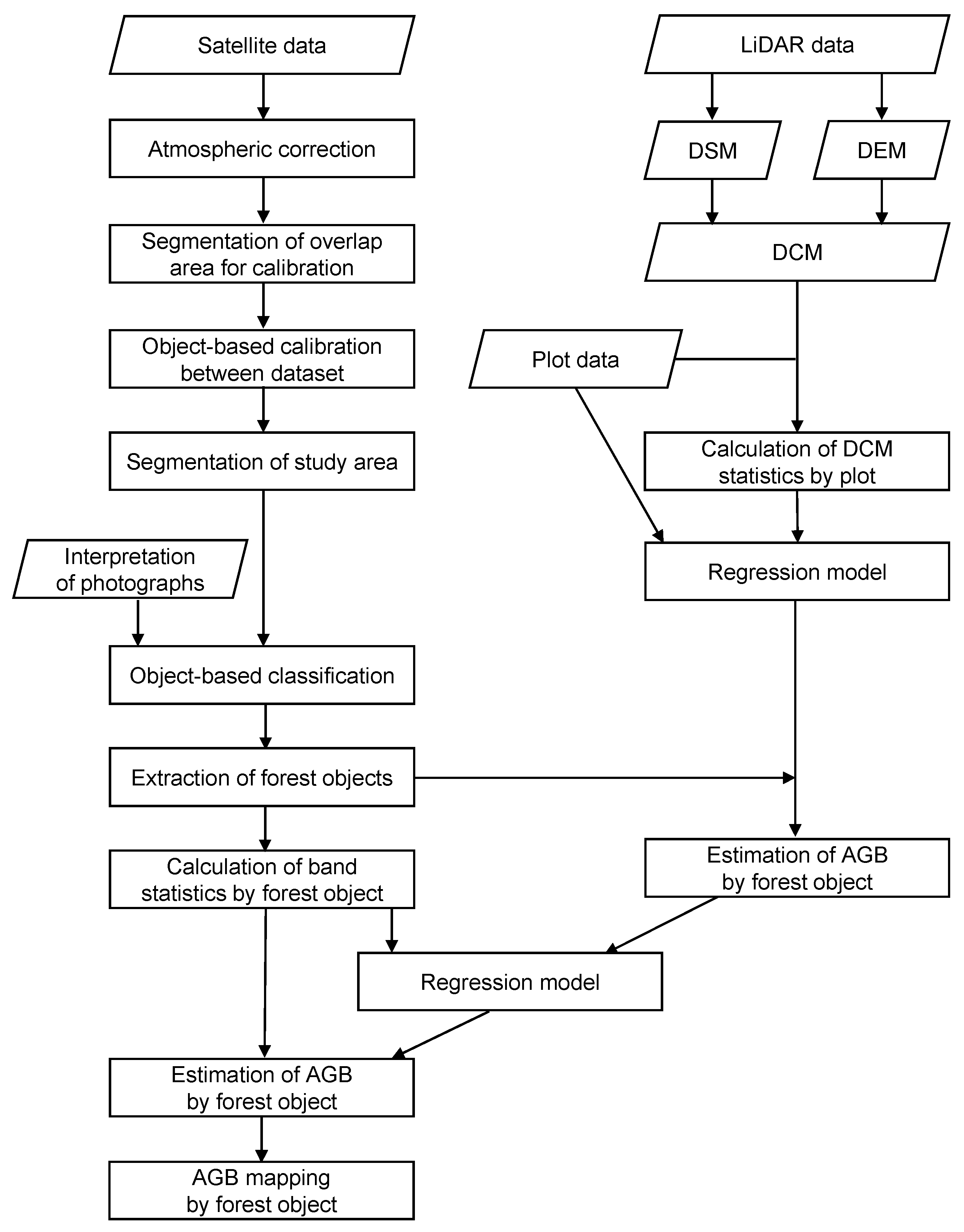
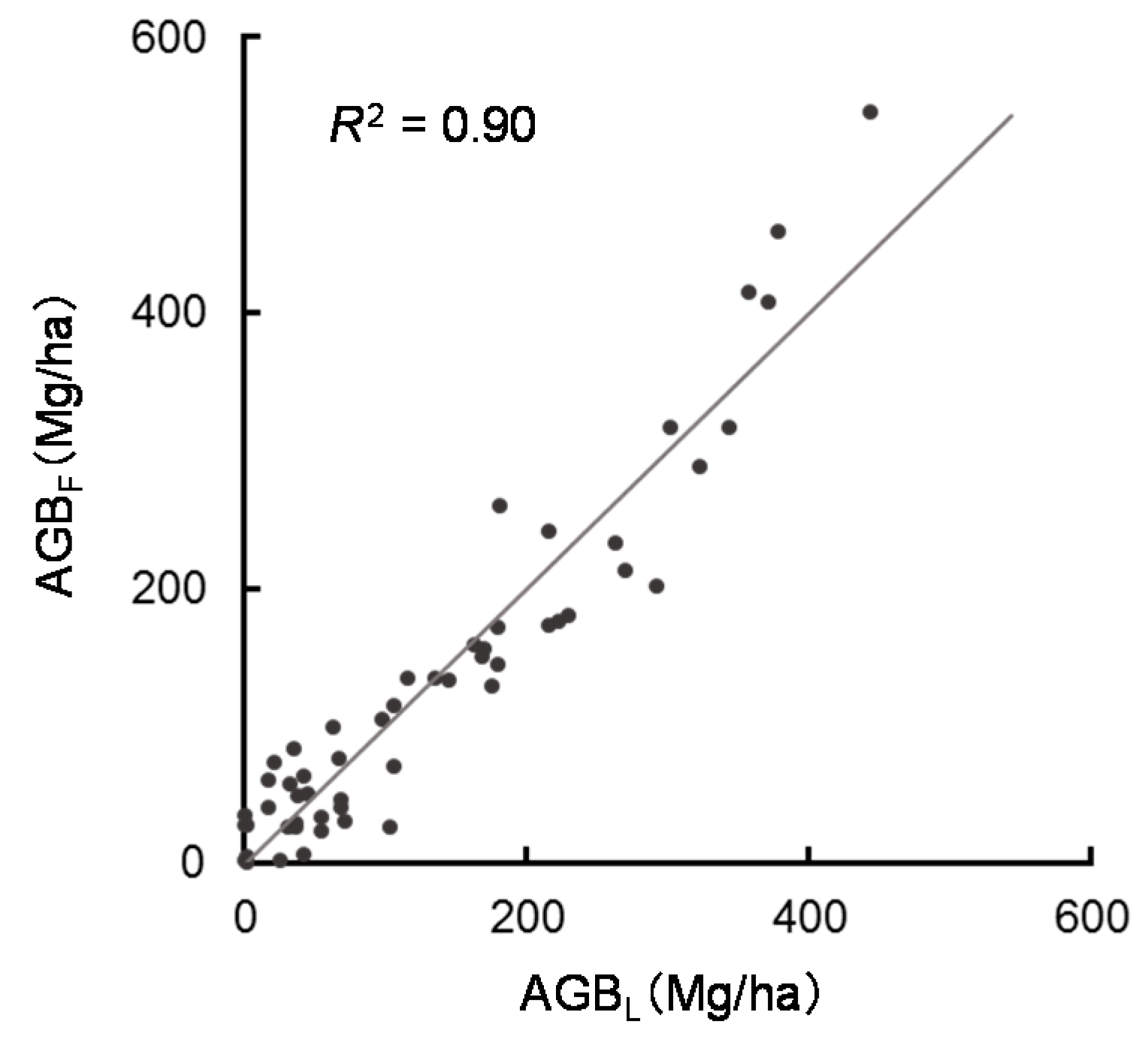
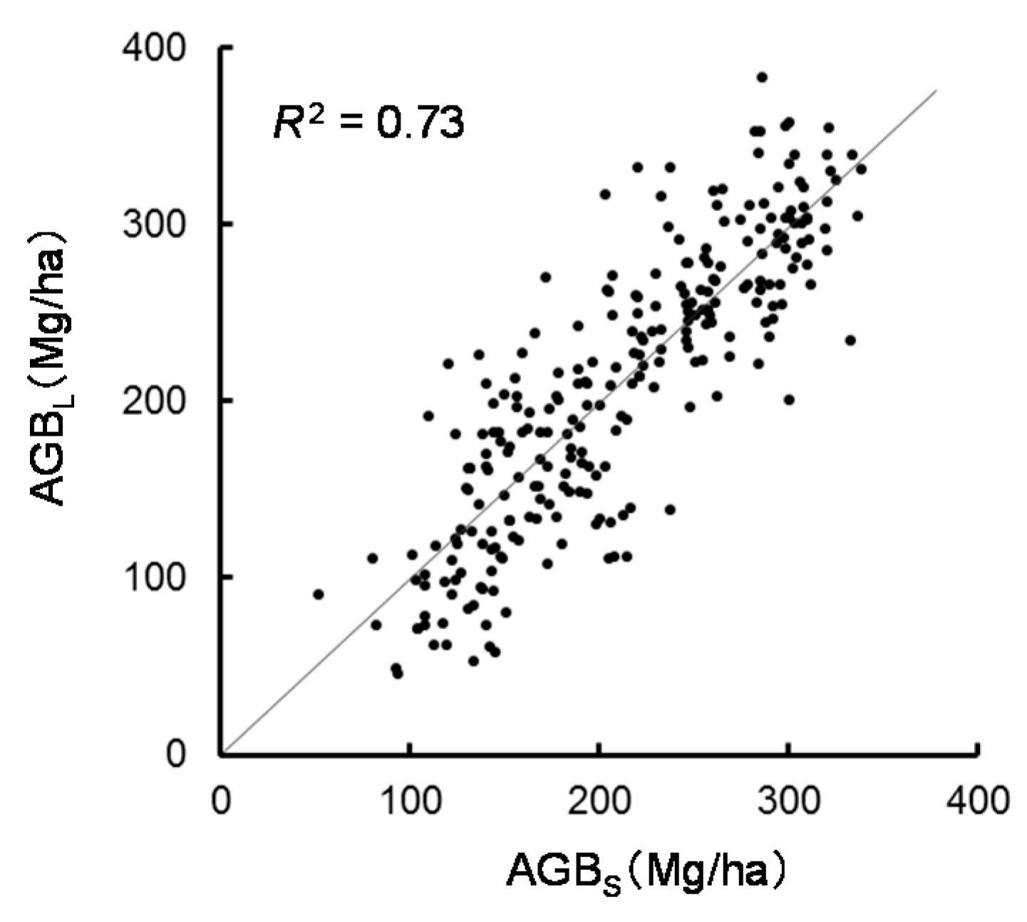
In this study, we aim to develop a method of estimating AGB in seasonal tropical forests by combining airborne LiDAR data with VHSR satellite data to obtain sampling data of forest carbon stock per unit area as the emission factor at a national level. This method can be used as an alternative of comprehensive field surveys to establish timely and reliable national forest inventory data. We used a two-step method: first, we studied the relationship between field-surveyed AGB and AGB predicted by the model derived from LiDAR data. Second, we created a multiple-regression model using AGB predicted by the LiDAR-based model as a dependent variable and the mean and standard deviation of the reflectance values of each band of the satellite data as the explanatory variables. This combination of methods is practical, as the cost of field survey is high and the cost of LiDAR survey is also relatively high. Thus, researchers and resource managers with limited budgets can estimate changes in the forest carbon stock per unit area as an emission factor based on the IPCC method by reducing the cost for forest inventory at a national level and compensating the lack of expertise necessary for large-scale surveys.

2. Materials and Methods

2.1. Study Area

The study area is located in Kampong Thom Province, central Cambodia, which is covered by three QuickBird images (12°34′57″ N to 12°46′54″ N, 105°14′22″ E to 105°30′24″ E, WGS84; Figure 1a,b). The area is 4.82 × 10⁴ ha. The whole study area was generally flat, with slopes <5°. In Cambodia, deforestation and forest degradation is caused by conversion to agricultural land and other uses, forest fires, and illegal logging, all of which result from local poverty and population growth. Forest cover has been decreasing since 1990, faster than most other parts of Southeast Asia. In particular, only half of the primary forests that existed in 1990 remain in 2010 [43]. This trend is the same in Kampong Thom. Although all forests are owned by the state, exploitation is carried out under various concessions for timber production, agribusiness (up to 10,000 ha), and homes and agricultural land for the poor [44].
In the study area, the annual average temperature is 27 °C, with relatively little monthly variation, and the annual precipitation is 1570 mm, with a dry season from November through March. The area features primary dry evergreen forest, secondary dry evergreen forest, deciduous dipterocarp forest, and regenerating forest. The primary dry evergreen forest has a canopy that can reach 40 m, with emergent, canopy, and lower-canopy layers. The basal area reaches 32.0 m2/ha and the forest is rich in species (Fisher’s α = 15.4). The dominant species are Dipterocarpus costatus, Vatica odorata subsp. brevipetiolata, and Anisoptera costata. In the secondary dry evergreen forest, some tall trees (with heights of about 40 m) remain, but the height range is wider than that of the primary forest. The basal area (38.9 m2/ha) and species diversity (α = 14.3) are as high as those of the primary dry evergreen forest. The dominant species is Irvingia malayana, but Goniothalamus multiovulatus and Sandoricum koetjape are also present. In the deciduous dipterocarp forest, which is characterized by a low basal area (9.7 m2/ha) and a low canopy height (<20 m), Dipterocarpus obtusifolius is the only tree species (α = 2.9) [45]. The regenerating forest is in the early stage of regeneration and is characterized by the very low basal area and the low canopy height (<10 m).

2.2. Remotely Sensed Data

We acquired VHSR satellite data, airborne LiDAR data, and digital aerial photographs to support our analysis.

2.2.1. VHSR Satellite Data

To cover the study area, we acquired three sets of overlapping QuickBird panchromatic and multispectral data, with respective ground resolutions of 0.61 and 2.44 m at nadir, collected on 27 and 30 November and 19 December 2011 (Figure 1b; Table 1). We selected the data in a short period of interval to reduce the risk of land cover changes and the influence of seasonality on reflectance from the canopy surface. The data were georegistered to the WGS 84 zone 51 datum with ground resolutions of 0.6 and 2.4 m using the nearest-neighbor method for resampling to maintain the original reflectance properties. Haze reduction and atmospheric correction were conducted using the ATCOR-2 (https://www.rese-apps.com/software/atcor/index.html) for ERDAS Imagine, and the grey-level values of all bands in each image were converted into reflectance values.

2.2.2. Airborne LiDAR Data

Airborne LiDAR data were acquired in January 2012 using the ALTM 3100 airborne laser terrain mapper (Teledyne Optech Inc., Vaughan, ON, Canada) in eight areas within the study area, which included all forest types (Figure 1c). The altitude of the helicopter was about 500 m, and the average flight speed was approximately 25 m/s. The frequency of the laser pulses was 100 kHz, and the scan frequency was 53 Hz. The maximum off-nadir scan angle was 12°. The beam divergence was 0.25 mrad. The sampling density of the laser scanning was about 26 pulses/m2. The density was very high in comparison with those used in other studies of LiDAR application, because we used the data to assess the effect of sampling density on the accurate estimation of forest carbon density in other studies [25]. The total area of the aerial survey was about 23.4 km2.
Though the sampling density of the laser scanning was high, the distribution of the last returns of the laser pulses from the ground was uneven, particularly in the evergreen forest, due to the large and dense crowns of some canopy trees. Our preliminary analysis using the point-cloud data (data not shown) suggested that it is not suitable to use a cell size smaller than 1 m for the DEM generated from the airborne LiDAR data. In addition, it is generally difficult for developing countries to acquire high-density LiDAR data due to its cost. Therefore, the DEM and the DSM were generated from the airborne LiDAR data of 1 m cell size in this study. The DEM was generated from the last returns of the laser pulses, and the DSM was generated by assigning the highest first-return value of the laser pulses for each cell as the cell’s value [46,47]. A digital canopy model (DCM) with a 1 m cell size, which shows the canopy height above the ground level, was then calculated by subtracting the DEM from the DSM.

2.2.3. Digital Aerial Photographs

True-color digital aerial photographs were obtained at the same time and in the same areas as the LiDAR measurements. Orthophotographs were generated from stereo-pair photos with a 0.5 m ground resolution. These orthophotographs were used to obtain training data for object-based land cover classification of the satellite data and to evaluate the classification results. The land cover type was interpreted from these orthophotographs by object, which includes the intersection of a 250 m × 250 m grid (total points = 766), which were produced by segmentation of the images in the Section 2.4.2 (Figure 2). Interpretation results of the objects at nearly half of the grid intersection points (384 points) were used as the training data for the object-based classification, and those of the objects at the remaining 382 points were used for verification. The training and verification points alternated in selection. Thus, the validation points were independent from the training dataset.

2.3. Field Survey

We established a total of 57 sample plots that measured either 30 m × 30 m (38) or 50 m × 50 m (19) in all forest types to create a LiDAR-based model for estimating AGB and determined the coordinates at the center of each plot using a global positioning system receiver (Germin eTrex 30) (Figure 1c). The average positioning accuracy of more than 30 min at each center was less than 5 m. We measured the diameter at breast height (DBH) of standing trees (DBH > 5 cm) in each plot and recorded their species. AGB of each tree was obtained from the allometric equation [48] based on the site conditions in the study area [49].
AGB = exp (−2.134 + 2.530 × ln (DBH))
AGB in the field sample plots (hereafter, AGBF) was estimated using the field-surveyed DBH values as inputs for Equation (1). Table 2 shows the summary statistics of the four main forest types in the field sample plots.

2.4. Data Analysis

Figure 3 shows the workflow of object-based mapping of AGB in tropical forests in Cambodia by combining satellite data and aerial LiDAR data as reference data.

2.4.1. Calibration of Satellite Data

After atmospheric correction, the digital number of the data in each band was converted to a reflectance value. The interval of acquisition of the images was less than 3 weeks, therefore, we considered that the influences of land use conversion and seasonal change was small. However, due to the difference between the angles of the observation and the solar elevation, the shadows of crowns on the canopy surface varied. Accordingly, we calibrated the satellite data to reduce this effect, as explained in the latter part of this section.
In the analysis of satellite data, it is difficult to match pixels of different dates due to the complicated relationship between the geometry of each crown and the observation angle. To solve this problem, we calibrated the reflectance values from the mean reflectance of the objects obtained by segmenting the data extracted from the overlapping areas in the different dates of the images. Satellite data were extracted from two overlap areas (Figure 1b). Both datasets were segmented using version 9.0.1 of eCognition software (http://www.ecognition.com/) using the multiresolution segmentation algorithm of Baatz and Schäpe [50]. The scale parameter for the segmentation was determined by comparing the statistics of the object size (mean and standard deviation) obtained from the segmentation results with different scale parameters to adjust to the minimum area of 1 ha used in the definition of forest by the Cambodian Forest Administration (scale parameter = 1000, shape parameter = 0.1, and compactness parameter = 0.5). We confirmed the results by using the digital aerial orthophotographs.
The mean reflectance of each object in each spectral band was calculated, and the values of the objects obtained from the data of 27 November and 19 December were linearly regressed by the normal least squares respectively, which served as the origin of the regression graph. The central image on 30 November was used as a reference images since it overlapped with the two other images. The regression equations obtained for each band were used to calibrate each pixel’s value from the satellite data on 27 November and 19 December. All data from the three dates were merged by band after the calibration.

2.4.2. Object-Based Classification of Satellite Data

Segmentation of the calibrated satellite data was conducted in the study area using the same scale parameters (scale parameter = 1000, shape parameter = 0.1, and compactness parameter = 0.5) used for the calibration of data to explain the minimum area of 1 ha used in the definition of forest by the Cambodian Forest Administration. Segmentation involves partitioning of an array of measurements based on their degree of homogeneity [51]. Multispectral pan-sharpened images of the four bands, which were prepared using ERDAS IMAGINE, and panchromatic image were used for the segmentation.
The objects obtained by this analysis were classified using a nearest neighbor algorithm in eCognition into primary dry evergreen forest, secondary dry evergreen forest, deciduous dipterocarp forest, regenerating forest, agricultural land, and bare land; the latter included built-up areas, clearcut sites, and unpaved roads. The classification used the mean and standard deviation of the reflectance value in each spectral band within an object and training data interpreted from the aerial orthophotographs. In general, it is considered that the mean of the reflectance value within an object is strongly related to land-cover type and that the standard deviation shows surface inhomogeneity. In this study, we use the generic allometric equation of Brown [48] to estimate AGB of individual tree. Ideally, local allometric equations should be developed for each forest type to improve the accuracy of the estimated AGB. However, we could not prepare local allometric equations for each forest type because of the cost and time requirements of such an exercise; we therefore used one generic allometric equation for all forest types, and the allometry was based on a single variable, namely DBH. In addition, we developed a single model to estimate AGB instead of models for the four main forest types in the next step, because the values of AGB by each forest type except the primary dry evergreen forest have a narrow range and it is difficult to develop four reliable models for all forest types. Then, we treat the forest area as one class in this study. The consequence of this approach was that in our final analysis, it was necessary to classify the area into forest versus non-forest types to extract the forest area, but initially, we classified the four forest types separately because they have different canopy characteristics and ground conditions. The mean and standard deviation of the reflectance in each spectral band of satellite data within an object were calculated to create the model for the estimation of AGB.

2.4.3. LiDAR-Based Model for AGB Estimation

Various linear and non-linear models have been developed for AGB estimation [16,27,52,53,54,55]. Some previous studies showed a good fitting of the linear model for biomass estimation [52,54,55]. In this study, we developed a linear model by means of multiple regression using LiDAR-derived height variables, namely the maximum (hmax), minimum (hmin), and mean (hmean) values of the sample plots from the DCM to estimate AGB (Mg/ha):
AGBF = β0 + β1 hmax + β2 hmin + β3 hmean
where β0, β1, β2, and β3 are regression coefficients. Here, we used variables in conjunction with the height in this study. They are very simple and basic variables in the LiDAR application to the estimation of AGB, and they have been used for various types and conditions of forests. We selected these simple variables while assuming that we use this model for REDD-plus. Ota et al. [25] indicated the mean value from the DCM was the most important variable to estimate AGB and canopy density was also significant. In this study, we used the mean value from the DCM and also the maximum and minimum values instead of canopy density. The mean DCM height was calculated from the DCM for each sample plot, and AGBF was obtained from the field data. Using these variables, we determined the coefficients by means of multiple regression.
Next, we calculated the maximum, minimum, and mean DCM heights using the objects obtained from the segmentation of the satellite data for the aerial survey area and used Equation (2) to estimate AGB for each object.

2.4.4. Development of a Model for AGB Estimation and Mapping Based on the Satellite Images

An object-based model to estimate AGB from the satellite data was developed by means of multiple regression using the LiDAR-derived AGB estimate (hereafter, AGBL) for each object as the dependent variable and the satellite data as the explanatory variables:
AGB L =   α 0 + k = 1 5 ( β k m k + γ k s k )
where k corresponds to the image band (k = 5 is the panchromatic data); α0, βk, and γk are the regression coefficients for band k; and mk and sk are the mean and standard deviation of the reflectance values by the object in band k. Because the mean and standard deviation are frequently used for the classification and extraction of stand attributes by means of object-based approach for VHSR images [56,57,58], we used these variables to develop the model. With this model, we calculated the AGB of all objects and the sample plots in the study area (hereafter, the two-step method), then evaluated the results by comparing the AGBF with the AGB of the sample plots predicted by the model based on the satellite image (hereafter, AGBS) by the two-step method. We also developed a regression model using the AGBF as the dependent variable, and the mean and standard deviation of the reflectance values by the object and the sample plot from satellite data as the explanatory variables (hereafter, the direct method), and evaluated the results by comparing the AGBF with the AGBS of the sample plots predicted by the direct method. Finally, we divided the results by density classes (in multiples of 50 Mg/ha), then mapped them.

3. Results

3.1. Calibration of the Satellite Data

Linear regression of the mean reflectance values of the objects obtained from the overlapping data of 30 November and 19 December (hereafter, the eastern overlap) and 30 November and 27 November (hereafter, the western overlap) gave regression equations with coefficients of determination of R2 = 0.75 to 0.93 and R2 = 0.96 to 0.99, respectively, and slopes of 1.08 to 1.19 and 0.95 to 0.98, respectively (Figure 4). After the calibration using these regression equations, the regression lines passed through the origin and the slopes were all 1.00 (data not shown). The calibration corrects the mean radiometry of the objects but not the radiometric variability when changes in observation conditions are likely to affect the degree of radiometric heterogeneity. Thus, we should recognize that the effect of the difference of the radiometric variability in the overlapped area between two images still remains after the calibration. The calibrated data for the three dates were merged by means of mosaic processing for each band.
Although the image dates were close together, differences in reflectance were evident. The images, which spanned an east–west width of about 10 km, were acquired on non-consecutive dates due to the satellite’s orbital pattern. In addition, the view angle difference of the sensor between the dates might lead to image differences. Thus, in large-scale biomass mapping using VHSR satellite data, it is necessary to account for discontinuity of data between dates. Land use change might cause further discontinuity, but the present study used a sufficiently short period, so this seems unlikely to have caused a problem.

3.2. Object-Based Classification of Satellite Data

Table 3 provides the error matrix for classification of the six land cover types with the 382 validation points. The overall classification accuracy for the six land cover classes was 77.0%. The primary dry evergreen forest had high accuracies with both user and producer accuracies of approximately 90%. In this type of forest, the satellite sensor observes only reflectance from the canopy surface due to the dense closed canopy, and this leads to high accuracies. The secondary dry evergreen forest had user and producer accuracies of 88.4% and 69.4%, respectively. This forest type was more often misclassified into one of the three other forest classes (i.e., omitted from the correct class) because its canopy was more heterogeneous. The dry dipterocarp forest had low user and producer accuracies (both less than 60%). The canopy of this forest type is open during the dry season (when our data were obtained) and the forest sometimes includes evergreen shrubs that further complicate identification of the tree canopy. The regenerating forest had relatively high user and producer accuracies (both >80%). Omission errors in this class tended to result from confusion with non-forest classes, and commission errors tended to result from the object being misclassified as secondary dry evergreen forest or dry dipterocarp forest. Agricultural land had user and producer accuracies that were both less than 60%. Although the user accuracy for bare land was also less than 60%, the producer accuracy was 74%. Omission and commission errors in these classes occurred as a result of confusion with almost all land cover classes except for the primary dry evergreen forest. In both classes, the object may include vegetation such as shrubs, crops, and any remaining trees. The relative proportions of such vegetation influence the classification result.
Overall classification accuracy improved to 92.9% when the primary dry evergreen forest, the secondary dry evergreen forest, the dry dipterocarp forest, and the regenerating forest were merged into a single forest category and the agricultural land and bare land were merged into a single non-forest category (Table 4). The forest class had user and producer accuracies of 98.4 and 93.5%, respectively. The non-forest class had user and producer accuracies of 65.1 and 89.1%, respectively.

3.3. LiDAR-Based Model for AGB Estimation

Table 5 summarizes the results of the multiple-regression analysis for the model in Equation (2) using the AGBF obtained from the field survey as the dependent variable and the LiDAR-derived variables (i.e., the maximum, minimum, and mean DCM heights) in each sample plot as the explanatory variables. The R2 and adjusted R2 values were both 0.90 (p < 0.001). Table 5 shows that the parameter estimate was greatest for the maximum and minimum DCM heights. The minimum DCM height is strongly related to the degree of closure of the forest canopy: it becomes nearly zero in an open-canopy forest, but is similar to the maximum DCM height in a closed-canopy forest. Therefore, AGB is affected both by the degree of closure of the forest canopy and by the size of the tallest trees in a forest. Minimum tree height should be 5 m according to the forest definition by the Cambodian government, therefore, the height of the trees in each plot is more than 8 m. Thus, the large negative intercept in the model was offset even in the open-canopy forest with small AGB.
AGBF values in the sample plots obtained from the field survey were plotted against the AGBL values of the sample plots predicted by the LiDAR-based model (Figure 5). The line passing through the origin to this relationship by least-squares regression analysis had a slope of 1.00 (R2 = 0.90, p < 0.001). The root-mean-square error (RMSE) was 38.7 Mg/ha.

3.4. The Model for AGB Estimation and Mapping Based on the Satellite Images

Table 6 shows the results of the multiple-regression analysis in Equation (3) using the AGBL predicted by the LiDAR-based model as the dependent variable and the mean and standard deviation of the reflectance values in each band of the satellite data for each object as the explanatory variables. R2 and adjusted R2 were 0.73 and 0.72, respectively (p < 0.001). AGBL values of the objects predicted by the LiDAR-based model were plotted against AGBS of the objects (Figure 6). With the regression line fitted through the origin using least-squares regression analysis, the slope was 1.00, and the RMSE was 42.8 Mg/ha (p < 0.001).
The comparison result between AGBF and AGBS in the sample plots determined by the two-step method is shown in Figure 7a. With the regression line fitted through the origin using least-squares regression analysis, the slope was 0.90 (R2 = 0.72). The RMSE was 69.4 Mg/ha. The AGBS model determined by the two-step method underestimated AGBF at high biomass and overestimated AGBF at low biomass. We also compared AGBF with AGBS in the sample plots determined by the direct method (Figure 7b). With the regression line fitted through the origin using least-squares regression analysis, the slope was 1.00 (R2 = 0.34). The RMSE was 99.6 Mg/ha. Figure 7b shows the weak correlation between AGBF and the AGBS derived from the direct method. These results indicated that the two-step method was more suitable than the direct method for estimating AGB.
We classified the AGBs of all objects of the forest by density (in multiples of 50 Mg/ha) and mapped them (Figure 8). It is clear from Figure 8 that relatively mature forest with high AGB is present in the eastern part of the study area. A flux tower has been established to measure carbon exchange and meteorological parameters in a tropical forest in this area [59,60], and the Cambodian Forestry Administration protects the area as experimental forest. However, conversion of forest into other land-use has occurred around the edges of the experimental forest. In the western part of the study area, there are residential areas where local people use the land for agriculture and use the forest as a source of fuel and construction wood. They also use forested areas to extend the area of agricultural land. As a result, the forest degrades continuously, and forests with low AGB are found in this area. Figure 8 clearly shows that most of the forests in this area have low AGB and that fragmentation of the forest dominates. AGB maps such as this one provide detailed information that can be used to support sustainable forest management at a local level.

4. Discussion

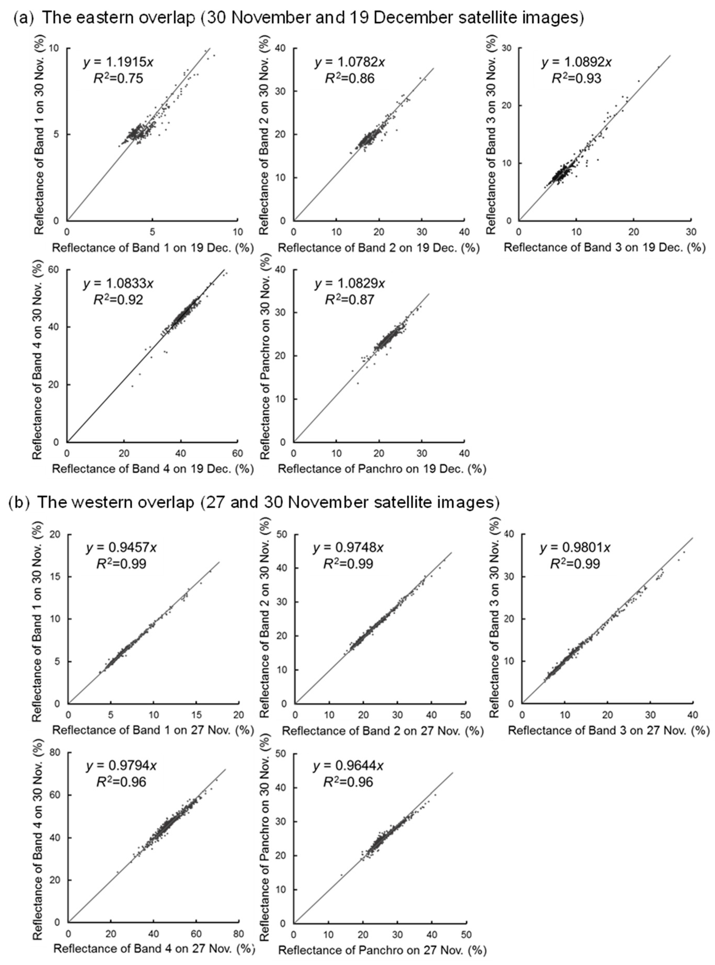
In this study, we assessed the viability of the two-step method for estimating AGB in tropical forests using LiDAR data and VHSR satellite data as the emission factor based on the IPCC method. When systematically obtaining such data from multistage sampling at a national level, the sampling rate must be taken into account, as the data depends largely on environmental and forest conditions. Multiple satellite images are occasionally needed to cover the area of interest for the mosaic processing to avoid the cloud problem or the east–west width of about 10 km covered by the satellite during each orbit. In this study, we used three satellite images that were acquired on close days, but not the same day. However, such images are not always available. When multiple satellite images are used, it is necessary to take account of the influences of the season and solar elevation, the difference in observation angles, and change in land use that occurred during the interval between images. The calibration method proposed in this study is not applicable when the images are acquired in different seasons or when there is a rapid change in land use. Changes in reflectance values caused by the seasonal influence in Landsat data were identified from the data with high temporal resolution such as MODIS [61,62]. In future research, it is necessary to confirm the applicability of the methods to the VHSR satellite images. Methods of detecting the change in land use were developed using time-series data from satellites such as Landsat in the previous studies [63,64,65]. Occurrences of land cover change need to be confirmed using such methods when multiple satellite images are used. There is the same problem in acquiring of LiDAR data. In the seasonal forest, the condition of the canopy changes in the dry season. Some cell values of the LiDAR-based DCM in the deciduous forest can be underestimated due to fallen leaves. The laser pulses return back only from the branches of the canopy. The tendency of this underestimate becomes stronger when the small size of cell is used for the DCM. Therefore, the beginning of the dry season is the best timing to acquire the LiDAR data in tropical seasonal forests, as leaves still remain in the trees. It is also necessary to consider the influences of changes in land use that occur in the interval between the image and the acquisition days of LiDAR.
Point-cloud data or percentiles from LiDAR data have often been used to estimate AGB [24,66], but we used DCM in the raster format. There was little difference between the DCM obtained from the raster format and that obtained from the point-cloud data. Ota et al. [25] developed a model to estimate aboveground carbon using point-cloud data in the same study area and the same LiDAR data, and showed that R2 was 0.92. The RMSE was slightly smaller than that of the model in this study. As a result, by simplifying using the DCM with 1 m cell size in place of the original point cloud data, the decrease in accuracy was small, so it is applicable to estimating forest carbon stock per unit area as an emission factor. In the tropics, with LiDAR, RMSEs ranging from 17 to 40 Mg/ha in forest carbon estimation or 10% of total carbon stock are reported [67]. Biomass is about twice as much as forest carbon stock. According to the analysis, AGB can be predicted with reasonable accuracy using the variables derived from LiDAR. Raster data has an advantage of estimating AGB in multistage sampling at a national level for REDD-plus implementation, because it is easier to process raster data than point-cloud data. However, the estimation accuracy depends on the cell size in the DCM, which in turn depends on the laser pulse density. When forests degrade due to the selective logging of large trees and other processes, the AGB will decrease and the gaps in the forest canopy will increase. In that case, the minimum DCM takes a small value when the value of the laser pulse density is larger than the reciprocal of the area of each gap, and the AGB of degraded forest is correctly estimated from the model. If the laser pulse density is lower than the above value, some gaps cannot be identified from the DCM and the AGB can be overestimated from the model. Optimal point density in the LiDAR measurement of various forest types and conditions need to be studied in future research.
In this study, we used the DCM in raster format, and the value of each cell showed the highest value in the cell. Therefore, we also needed to take account of the cell size when we used the raster data. When part of the crown is included in a given cell around the rim of a gap, that cell takes the value of the crown height even if the ground occupies most of the cell. Since the frequency of such cells increases when the cell size is large, some gaps cannot be identified in the DCM and the estimates of the mean and minimum DCM increase. However, the number of such cells is usually very small compared to the total number of cells. Therefore, the influence of cell size of the model is considered to be relatively small. As the DCM represents only the canopy surface, information from understorey strata is lost. Thus, it is a concern that this will lead to underestimation of the AGB, because it is not enough to estimate the AGB of standing trees in the understorey strata. However, the RMSE of our model was almost the same as that of the model developed using point-cloud data. It is suggested that standing trees in the understorey strata account for a small ratio in AGB. It should also be noted that information on the understorey strata obtained from point-cloud data is limited when the canopy layer is closed.
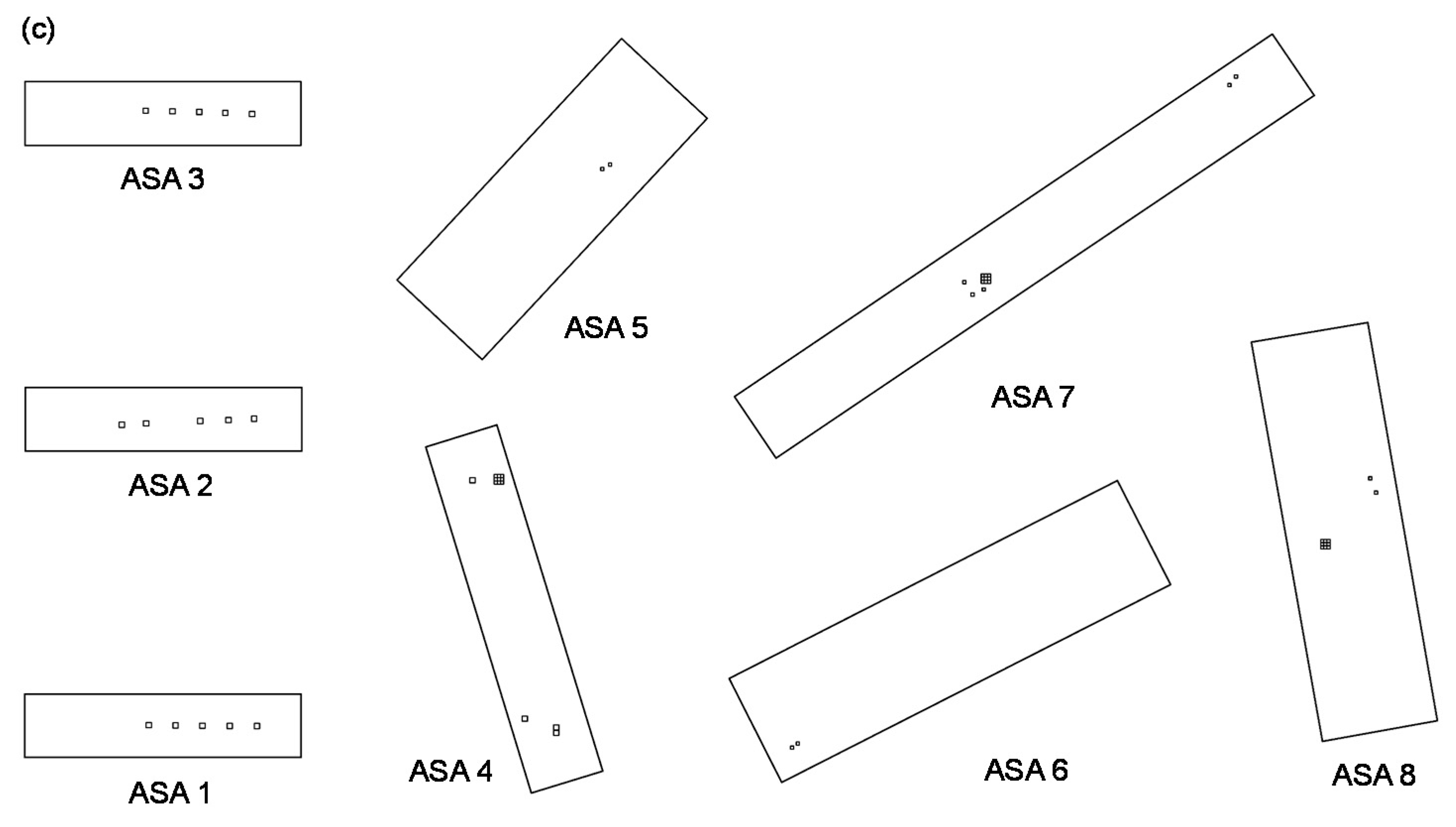
When developing a model to estimate AGB in tropical forests, it is necessary to consider the problem of the plot size. In LiDAR measurement, we retrieved the three-dimensional structure of the canopy and estimated AGB mainly from the canopy height. Generally, a part of crown of the tree which stands outside of the plot is included in the plot, and that of the tree which stands inside of the plot sometimes exists outside of the plot. This leads to overestimation or underestimation of the AGB. In addition, problems can arise from the combination of small plots with imperfect positioning with a low-end GPS device. When plot size is small, the influence is large. Establishing large plots can reduce the influence, but it is difficult to establish the required number of plots for developing the model with accurate differential positioning, particularly in tropical forests.
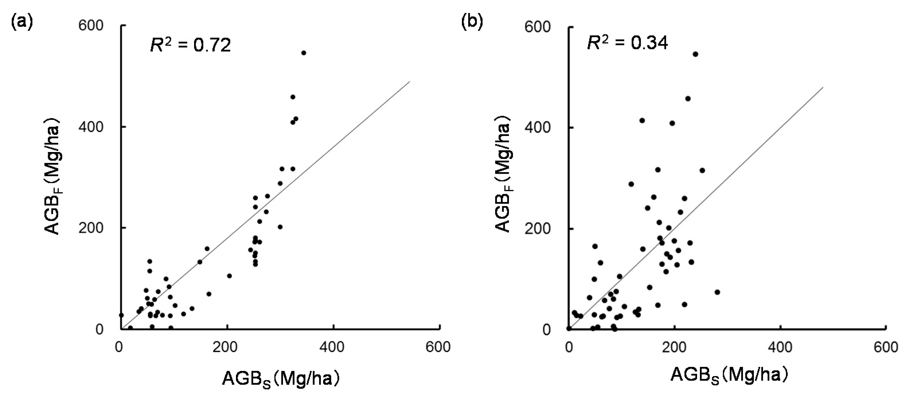
We showed that the satellite-based model for the AGB estimation using the two-step method was superior to that using the direct method, when compared the RSMEs. However, the saturation of the AGB values of about 330 Mg/ha in the two-step method and about 200 Mg/ha in the direct method occurred. In general, the optical satellite sensor observes the canopy surface of forest areas. Therefore, it is thought that the difference in individual tree sizes becomes unclear when the forest canopy is closed.
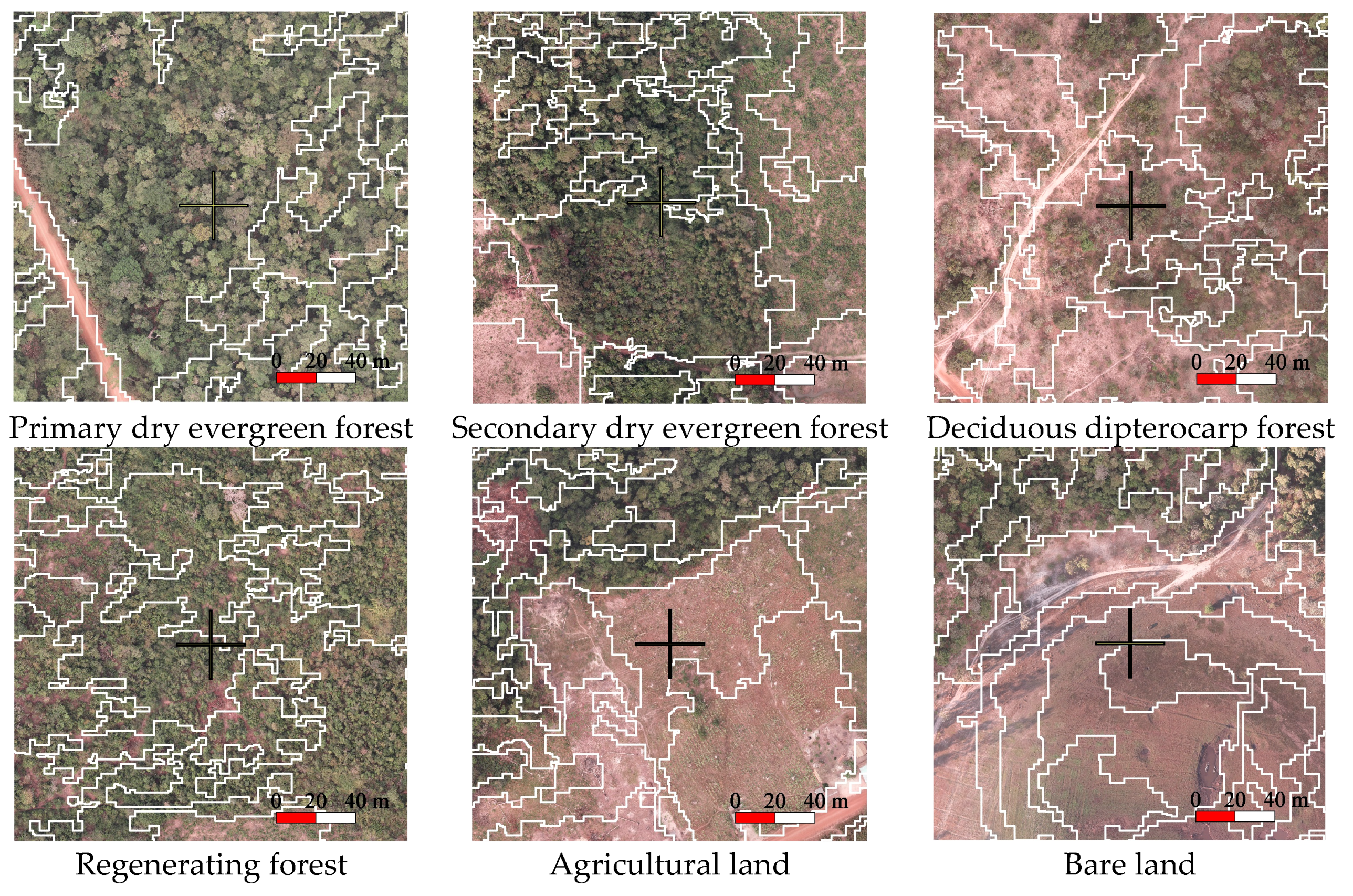
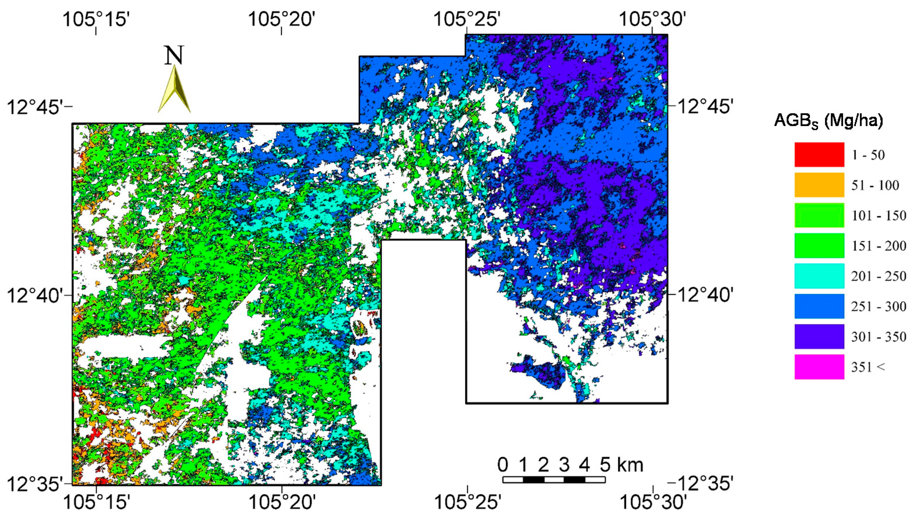
AGB maps produced using the method in the present study provide a clear picture of forest conditions at a local level. Object-based classification facilitates the creation of such maps using geographic information system software, and the data directly supports the planning of forest management activities. The object-based approach is used in the expectation that it will divide the image into relatively uniform and thematically significant groups of pixels [30]. In recent years, an automated parameterization method for multi-scale image segmentation on multiple layers has been developed [68]. Advances in object-based approaches have potential to expand the use of VHSR satellite images for land cover classification. On the other hand, the problem of the land use not being the same as the land cover means it is difficult to apply fully automatic method in the object-based approach. In addition, the minimum mapping unit differs greatly from the area used to define a patch of forest in many developing countries. Due to the difference between the two scales, it is difficult to distinguish forest degradation from land cover change cutting the small area of the forests [69]. In particular, the land use pattern around residential areas is complicated, and two land cover classes are frequently mixed. For example, when crops are cultivated in an open forest, the land use is considered to agriculture. However, satellite sensors simultaneously observe a mixture of reflectance from tree crowns, crops, and soil, which causes misclassification. It should be noted that such misclassification often occurs in highly populated areas.

5. Conclusions

REDD-plus is considered an important measure for the mitigation of climate change, and a reliable monitoring method is essential to establish a reference emission level to evaluate the emission reductions achieved by REDD-plus activities. At a national level, a combination of remote sensing and ground-based inventory data can effectively determine carbon stock changes. However, due to inaccessibility to forests and lack of expertise required for large-scale surveys, it is occasionally difficult to design and implement field surveys. In this study, we developed a method of estimating AGB in seasonal tropical forests by combining airborne LiDAR data with VHSR satellite data to obtain sampling data of forest carbon stock per unit area as the emission factor at a national level. This method can be used as an alternative to comprehensive field surveys to establish timely and reliable national forest inventory data. Our results suggest that this approach can provide the forest carbon stock per unit area values required to support REDD-plus.

Acknowledgments

This study was conducted as part of the “Technology development for circulatory food production systems responsive to climate change” project and the “Support promotion of REDD+ activities by private sector” project and was supported by the Ministry of Agriculture, Forestry and Fisheries, and the Forestry Agency, Japan. We thank the staff of the Forestry Administration in Cambodia for their valuable assistance during the field surveys.

Author Contributions

Yasumasa Hirata conceived and designed the methodology of the study; Naoyuki Furuya and Hideki Saito performed field survey and data analysis; Chealy Pak, Chivin Leng, Heng Sokh, and Vuthy Ma liaised to obtain permission to research in Cambodian forest and provided significant knowledge about forests in Cambodia, and arranged and performed field survey; Tsuyoshi Kajisa, Tetsuji Ota, Nobuya Mizoue reviewed the methodology of the study and gave comments and suggestions to the manuscript.

Conflicts of Interest

The authors declare no conflict of interest.

References

  1. Smith, P.; Bustamante, M.; Ahammad, H.; Clark, H.; Dong, H.; Elsiddig, E.A.; Haberl, H.; Harper, R.; House, J.; Jafari, M.; et al. Agriculture, Forestry and Other Land Use (AFOLU). In Climate Change 2014: Mitigation of Climate Change; Edenhofer, O., Pichs-Madruga, R., Sokona, Y., Farahani, E., Kadner, S., Seyboth, K., Seyboth, A., Eds.; Cambridge University Press: New York, NY, USA, 2014; pp. 811–922. ISBN 978-1-107-05821-7. [Google Scholar]
  2. Aalde, H.; Gonzalez, P.; Gytarsky, M.; Krug, T.; Kurz, W.A.; Lasco, R.D.; Martino, D.L.; McConkey, B.G.; Ogle, S.; Paustian, K.; et al. IPCC Chapter 2: Generic methodologies applicable to multiple land-use categories. In 2006 IPCC Guidelines for National Greenhouse Gas Inventories, Agriculture, Forestry and Other Land Use; Eggleston, H.S., Buendia, L., Miwa, K., Ngara, T., Tanabe, K., Eds.; IGES: Hayama, Japan, 2006; Volume 4, pp. 2.1–2.59. ISBN 4-88788-032-4. [Google Scholar]
  3. Guinea, P.N.; Rica, C. Reducing Emissions from Deforestation in Developing Countries: Approaches to Stimulate Action; FCCC/SBSTA/2009/L.19/Add.1; UNFCCC: Bonn, Germany, 2009; p. 2. [Google Scholar]
  4. UNFCCC. Cost of Implementing Methodologies and Monitoring Systems Relating to Estimates of Emissions from Deforestation and Forest Degradation, the Assessment of Carbon Stocks and Greenhouse Gas Emissions from Changes in Forest Cover, and the Enhancement of Forest Carbon Stocks; FCCC/TP/2009/1; UNFCCC: Bonn, Germany, 2009; pp. 17–36. [Google Scholar]
  5. Mascaro, J.; Asner, G.P.; Muller-Landau, H.C.; van Breugel, M.; Hall, J.; Dahlin, K. Controls over aboveground forest carbon density on Barro Colorado Island, Panama. Biogeosciences 2011, 8, 1615–1629. [Google Scholar] [CrossRef] [Green Version]
  6. Saatchi, S.S.; Harris, N.L.; Brown, S.; Lefsky, M.; Mitchard, E.T.A.; Salas, W.; Zutta, B.R.; Buermann, W.; Lewis, S.L.; Hagen, S.; et al. Benchmark map of forest carbon stocks in tropical regions across three continents. Proc. Natl. Acad. Sci. USA 2011, 108, 9899–9904. [Google Scholar] [CrossRef] [PubMed]
  7. Hudak, A.T.; Crookston, N.L.; Evans, J.S.; Falkowski, M.J. Regression modeling and mapping of coniferous forest basal area and tree density from discrete-return lidar and multispectral satellite data. Can. J. Remote Sens. 2006, 32, 126–138. [Google Scholar] [CrossRef]
  8. Kauranne, T.; Joshi, A.; Gautam, B.; Manandhar, U.; Nepal, S.; Peuhkurinen, J.; Hämäläinen, J.; Junttila, V.; Gunia, K.; Latva-Käyrä, P.; et al. LiDAR-assisted multi-source program (LAMP) for measuring above ground biomass and forest carbon. Remote Sens. 2017, 9, 154. [Google Scholar] [CrossRef]
  9. Saarela, S.; Holm, S.; Grafström, A.; Schnell, S.; Næsset, E.; Gregoire, T.G.; Nelson, R.F.; Ståhl, G. Hierarchical model-based inference for forest inventory utilizing three sources of information. Ann. For. Sci. 2016, 73, 895–910. [Google Scholar] [CrossRef]
  10. Ståhl, G.; Saarela, S.; Schnell, S.; Holm, S.; Breidenbach, J.; Healey, S.P.; Patterson, P.L.; Magnussen, S.; Næsset, E.; McRoberts, R.E.; et al. Use of models in large-area forest surveys: Comparing model-assisted, model-based and hybrid estimation. For. Ecosyst. 2016, 3. [Google Scholar] [CrossRef]
  11. Magnussen, S.; Boudewyn, P. Derivations of stand heights from airborne laser scanner data with canopy-based quantile estimators. Can. J. For. Res. 1998, 28, 1016–1031. [Google Scholar] [CrossRef]
  12. Næsset, E. Determination of mean tree height of forest stands using airborne laser scanner data. ISPRS J. Photogramm. Remote Sens. 1997, 52, 49–56. [Google Scholar] [CrossRef]
  13. Næsset, E.; Bjerknes, K.-O. Estimating tree heights and number of stems in young stands using airborne laser scanner data. Remote Sens. Environ. 2001, 78, 328–340. [Google Scholar] [CrossRef]
  14. St-Onge, B.; Treitz, P.; Wulder, M.A. Tree and canopy height estimation with scanning LiDAR. In Remote Sensing of Forest Environments—Concepts and Case Studies; Wulder, M.A., Franklin, S.E., Eds.; Kluwer Academic Publishers: Dordrecht, The Netherlands, 2003; pp. 489–509. ISBN 978-1-4615-0306-4. [Google Scholar]
  15. Maltamo, M.; Mustonen, K.; Hyyppä, J.; Pitkänen, J.; Yu, X. The accuracy of estimating individual tree variables with airborne laser scanning in a boreal nature reserve. Can. J. For. Res. 2004, 34, 1791–1801. [Google Scholar] [CrossRef]
  16. Næsset, E. Estimating timber volume of forest stands using airborne laser scanner data. Remote Sens. Environ. 1997, 61, 246–253. [Google Scholar] [CrossRef]
  17. Hyyppä, J.; Inkinen, M. Detecting and estimating attributes for single trees using laser scanner. Photogramm. J. Finl. 1999, 16, 27–42. [Google Scholar]
  18. Hyyppä, J.; Kelle, O.; Lehikoinen, M.; Inkinen, M. A segmentation-based method to retrieve stem volume estimates from 3-D tree height models produced by laser scanners. IEEE Trans. Geosci. Remote Sens. 2001, 39, 969–975. [Google Scholar] [CrossRef]
  19. McCombs, J.W.; Roberts, S.D.; Evans, D.L. Influence of fusing LiDAR and multispectral imagery on remotely sensed estimates of stand density and mean tree height in a managed loblolly pine plantation. For. Sci. 2003, 49, 457–466. [Google Scholar]
  20. Persson, Å.; Holmgren, J.; Söderman, U. Detecting and measuring individual trees using an airborne laser scanner. Photogramm. Eng. Remote Sens. 2002, 68, 925–932. [Google Scholar]
  21. Takahashi, T.; Yamamoto, K.; Senda, Y.; Tsuzuku, M. Predicting individual stem volumes of sugi (Cryptomeria japonica D. Don) plantations in mountainous areas using small-footprint airborne LiDAR. J. For. Res. 2005, 10, 305–312. [Google Scholar] [CrossRef]
  22. Asner, G.P.; Mascaro, J.; Muller-Landau, H.C.; Vieilledent, G.; Vaudry, R.; Rasamoelina, M.; Hall, J.S.; van Breugel, M. A universal airborne LiDAR approach for tropical forest carbon mapping. Oecologia 2012, 168, 1147–1160. [Google Scholar] [CrossRef] [PubMed]
  23. Asner, G.P.; Mascaro, J. Mapping tropical forest carbon: Calibrating plot estimates to a simple LiDAR metric. Remote Sens. Environ. 2014, 140, 614–624. [Google Scholar] [CrossRef]
  24. Ioki, K.; Tsuyuki, S.; Hirata, Y.; Phua, M.H.; Wong, W.V.C.; Ling, Z.-Y.; Saito, H.; Takao, G. Estimating above-ground biomass of tropical rainforest of different degradation levels in Northern Borneo using airborne LiDAR. For. Ecol. Manag. 2014, 328, 335–341. [Google Scholar] [CrossRef]
  25. Ota, T.; Kajisa, T.; Mizoue, N.; Yoshida, S.; Takao, G.; Hirata, Y.; Furuya, N.; Sano, T.; Ponce-Hernandez, R.; Ahmed, O.S.; et al. Estimating aboveground carbon using airborne LiDAR in Cambodian tropical seasonal forests for REDD+ implementation. J. For. Res. 2015, 20, 484–492. [Google Scholar] [CrossRef]
  26. Andersen, H.E.; Strunk, J.; Temesgen, H. Using airborne light detection and ranging as a sampling tool for estimating forest biomass resources in the Upper Tanana Valley of Interior Alaska. West. J. Appl. For. 2011, 26, 157–164. [Google Scholar]
  27. Næsset, E. Predicting forest stand characteristics with airborne scanning laser using a practical two-stage procedure and field data. Remote Sens. Environ. 2002, 80, 88–99. [Google Scholar] [CrossRef]
  28. Eckert, S. Improved forest biomass and carbon estimations using texture measures from WorldView-2 satellite data. Remote Sens. 2012, 4, 810–829. [Google Scholar] [CrossRef]
  29. Hilker, T.; Wulder, M.A.; Coops, N.C. Update of forest inventory data with lidar and high spatial resolution satellite data. Can. J. Remote Sens. 2008, 34, 5–12. [Google Scholar] [CrossRef]
  30. Blaschke, T. Object based image analysis for remote sensing. ISPRS J. Photogramm. Remote Sens. 2010, 65, 2–16. [Google Scholar] [CrossRef]
  31. Clark, D.B.; Castro, C.S.; Alvarado, L.D.A.; Read, J.M. Quantifying mortality of tropical rain forest trees using high-spatial-resolution satellite data. Ecol. Lett. 2004, 7, 52–59. [Google Scholar] [CrossRef]
  32. Heenkenda, M.K.; Joyce, K.E.; Maier, S.W. Mangrove tree crown delineation from high-resolution imagery. Photogramm. Eng Remote Sens. 2015, 81, 471–479. [Google Scholar] [CrossRef]
  33. Hirata, Y.; Tsubota, Y.; Sakai, A. Allometric models of DBH and crown area derived from QuickBird panchromatic data in Cryptomeria japonica and Chamaecyparis obtusa stands. Int. J. Remote Sens. 2009, 30, 5071–5088. [Google Scholar] [CrossRef]
  34. Strahler, A.H.; Woodcock, C.E.; Smith, J.A. On the nature of models in remote sensing. Remote Sens. Environ. 1986, 20, 121–139. [Google Scholar] [CrossRef]
  35. Ehlers, M.; Gähler, M.; Janowsky, R. Automated analysis of ultra high resolution remote sensing data for biotope type mapping: New possibilities and challenge. ISPRS J. Photogramm. Remote Sens. 2003, 57, 315–326. [Google Scholar] [CrossRef]
  36. Coutern, P.; Barbier, N.; Deblauwe, V.; Pélissier, R.; Ploton, P. Texture analysis of very high spatial resolution optical images as a way to monitor vegetation and forest biomass in the tropics. In Geospatial Information Systems for Multi-Scale Forest Biomass Assessment and Monitoring in the Hindu Kush Himalayan Region; ICIMOD: Kathmandu, Nepal, 2015; pp. 157–164. [Google Scholar]
  37. Bastin, J.-F.; Barbier, N.; Barbier, N.; Coutern, P.; Adams, B.; Shapiro, A.; Bogaert, J.; De Cannire, C. Aboveground biomass mapping of African forest mosaics using canopy texture analysis: Toward a regional approach. Ecol. Appl. 2014, 24, 1984–2001. [Google Scholar] [CrossRef] [PubMed]
  38. Hay, G.J.; Marceau, D.; Dube, P.; Bouchard, A. A multiscale framework for landscape analysis: Object-specific analysis and upscaling. Landsc. Ecol. 2001, 16, 471–490. [Google Scholar] [CrossRef]
  39. Platt, R.V.; Schoennagel, T. An object-oriented approach to assessing changes in tree cover in the Colorado Front Range 1938–1999. For. Ecol. Manag. 2009, 258, 1342–1349. [Google Scholar] [CrossRef]
  40. Hussin, Y.A.; Gilani, H.; van Leeuwen, L.; Murthy, M.S.R.; Shah, R.; Baral, S.; Tsendbazar, N.-E.; Shrestha, S.; Shah, S.K.; Qamer, F.M. Evaluation of object-based image analysis techniques on very high-resolution satellite image for biomass estimation in a watershed of hilly forest of Nepal. Appl. Geomath. 2014, 6, 59–68. [Google Scholar] [CrossRef]
  41. Antonarakis, A.S.; Richards, K.S.; Brasington, J. Object-based land cover classification using airborne LiDAR. Remote Sens. Environ. 2008, 112, 2988–2998. [Google Scholar] [CrossRef]
  42. Ke, Y.; Quackenbush, L.J.; Im, J. Synergistic use of QuickBird multispectral imagery and LIDAR data for object-based forest species classification. Remote Sens. Environ. 2010, 114, 1141–1154. [Google Scholar] [CrossRef]
  43. Food and Agriculture Organization. Global Forest Resources Assessment 2015—Country Report Cambodia; FAO: Rome, Italy, 2014; p. 23. [Google Scholar]
  44. Ehara, M.; Hyakumura, K.; Nomura, H.; Matsuura, T.; Sokh, H.; Leng, C. Identifying characteristics of households affected by deforestation in their fuelwood and non-timber forest product collections: Case study in Kampong Thom Province, Cambodia. Land Use Policy 2016, 52, 92–102. [Google Scholar] [CrossRef]
  45. Tani, A.; Ito, E.; Kanzaki, M.; Ohta, S.; Khron, S.; Pith, P.; Tith, B.; Pol, S.; Lim, S. Principal forest types of three regions of Cambodia: Kampong Thom, Kratie, and Mondolkiri. In Forest Environments in the Mekong River Basin; Sawada, H., Araki, M., Chappell, N.A., LaFrankie, J.V., Shimizu, A., Eds.; Springer: Tokyo, Japan, 2007; pp. 210–213. ISBN 978-4-431-46503-4. [Google Scholar]
  46. Duan, Z.; Zhao, D.; Zeng, Y.; Zhao, Y.; Wu, B.; Zhu, J. Assessing and correcting topographic effects on forest canopy height retrieval using airborne LiDAR data. Sensors 2015, 15, 12133–12155. [Google Scholar] [CrossRef] [PubMed]
  47. Hirata, Y.; Furuya, N.; Suzuki, M.; Yamamoto, H. Airborne laser scanning in forest management: Individual tree identification and laser pulse penetration in a stand with different levels of thinning. For. Ecol. Manag. 2009, 258, 752–760. [Google Scholar] [CrossRef]
  48. Brown, S. Estimating Biomass and Biomass Change of Tropical Forests, a Primer; Food and Agriculture Organization (FAO): Rome, Italy, 1997; ISBN 92-5-103955-0. [Google Scholar]
  49. Monda, K. Analysis of permanent sample plot data. In REDD-plus Cookbook; Hirata, Y., Takao, G., Sato, T., Toriyama, J., Eds.; REDD Research and Development Center, Forestry and Forest Products Research Institute: Tsukuba, Japan, 2012; pp. 120–123. ISBN 978-4-905304-15-9. [Google Scholar]
  50. Baatz, M.; Schäpe, A. Multiresolution segmentation-an optimization approach for high quality multi-scale image segmentation. In Angewandte Geographische Informationsverarbeitung; Strobl, J., Blaschke, T., Griesebner, G., Eds.; Wichmann-Verlag: Heidelberg, Germany, 2000; pp. 12–23. ISBN 387907349X. [Google Scholar]
  51. Blaschke, T.; Hay, G.J.; Kelly, M.; Lang, S.; Hofmann, P.; Addink, E.; Queiroz Feitosa, R.; van der Meer, F.; van der Werff, H.; van Coillie, F.; et al. Geographic Object-Based Image Analysis—Towards a new paradigm. ISPRS J. Photogramm. Remote Sens. 2014, 87, 180–191. [Google Scholar] [CrossRef] [PubMed]
  52. Drake, J.B.; Dubayah, R.O.; Knox, R.G.; Clark, D.B.; Blair, J.B. Sensitivity of large-footprint lidar to canopy structure and biomass in a neotropical rainforest. Remote Sens. Environ. 2002, 81, 378–392. [Google Scholar] [CrossRef]
  53. Magnusson, M.; Fransson, J.E.S.; Holmgren, J. Effects on estimation accuracy of forest variables using different pulse density of laser data. For. Sci. 2007, 53, 619–626. [Google Scholar]
  54. Popescu, S.C. Estimating biomass of individual pine trees using airborne lidar. Biomass Bioenergy 2007, 31, 646–655. [Google Scholar] [CrossRef]
  55. Zhao, K.; Popescu, S.; Nelson, R. Lidar remote sensing of forest biomass: A scale-invariant estimation approach using airborne lasers. Remote Sens. Environ. 2009, 113, 182–196. [Google Scholar] [CrossRef]
  56. Atzberger, C. Object-based retrieval of biophysical canopy variables using artificial neural nets and radiative transfer models. Remote Sens. Environ. 2004, 93, 53–67. [Google Scholar] [CrossRef]
  57. Chubey, M.S.; Franklin, S.E.; Wulder, M.A. Object-based Analysis of Ikonos-2 Imagery for Extraction of Forest Inventory Parameters. Photogramm. Eng. Remote Sens. 2006, 72, 383–394. [Google Scholar] [CrossRef]
  58. Yu, Q.; Gong, P.; Clinton, N.; Biging, G.; Kelly, M.; Schirokauer, D. Object-based detailed vegetation classification with airborne high spatial resolution remote sensing imagery. Photogramm. Eng. Remote Sens. 2006, 72, 799–811. [Google Scholar] [CrossRef]
  59. Nobuhiro, T.; Shimizu, A.; Kabeya, N.; Tamai, K.; Ito, E.; Araki, M.; Kubota, T.; Tsuboyama, Y.; Chann, S. Evapotranspiration during the late rainy season and middle of the dry season in the watershed of an evergreen forest area, central Cambodia. Hydrol. Process. 2008, 22, 1281–1289. [Google Scholar] [CrossRef]
  60. Tamai, K.; Shimizu, A.; Nobuhiro, T.; Kabeya, N.; Chann, S.; Keth, N. Measurements of wind speed, direction, and vertical profiles in an evergreen forest in central Cambodia. In Forest Environments in the Mekong River Basin; Sawada, H., Araki, M., Chappell, N.A., LaFrankie, J.V., Shimizu, A., Eds.; Springer: Tokyo, Japan, 2007; pp. 87–96. ISBN 978-4-431-46503-4. [Google Scholar]
  61. Hilker, T.; Wulder, M.A.; Coops, N.C.; Seitz, N.; White, J.C.; Gao, F.; Masek, J.G.; Stenhouse, G. Generation of dense time series synthetic Landsat data through data blending with MODIS using a spatial and temporal adaptive reflectance fusion model. Remote Sens. Environ. 2009, 113, 1988–1999. [Google Scholar] [CrossRef]
  62. Walker, J.J.; De Beurs, K.M.; Wynne, R.H.; Gao, F. Evaluation of Landsat and MODIS data fusion products for analysis of dryland forest phenology. Remote Sens. Environ. 2012, 117, 381–392. [Google Scholar] [CrossRef]
  63. Cohen, W.B.; Yang, Z.; Kennedy, R.E. Detecting trends in forest disturbance and recovery using yearly Landsat time series: 2. TimeSync—Tools for calibration and validation. Remote Sens. Environ. 2010, 114, 2911–2924. [Google Scholar] [CrossRef]
  64. Huang, C.; Goward, S.N.; Masek, J.G.; Thomas, N.; Zhu, Z.; Vogelmann, J.E. An automated approach for reconstructing recent forest disturbance history using dense Landsat time series stacks. Remote Sens. Environ. 2010, 114, 183–198. [Google Scholar] [CrossRef]
  65. Kennedy, R.E.; Yang, Z.; Cohen, W.B. Detecting trends in forest disturbance and recovery using yearly Landsat time series: 1. LandTrendr—Temporal segmentation algorithms. Remote Sens. Environ. 2897, 114, 2897–2910. [Google Scholar] [CrossRef]
  66. Kronseder, K.; Ballhorn, U.; Böhmc, V.; Sieger, F. Above ground biomass estimation across forest types at different degradation levels in Central Kalimantan using LiDAR data. Int. J. Appl. Earth Obs. Geoinf. 2012, 18, 37–48. [Google Scholar] [CrossRef]
  67. Mascaro, J.; Detto, M.; Asner, G.P.; Muller-Landau, H.C. Evaluating uncertainty in mapping forest carbon with airborne LiDAR. Remote Sens. Environ. 2011, 115, 3770–3774. [Google Scholar] [CrossRef]
  68. Drăguţ, L.; Csillik, O.; Eisank, C.; Tiede, D. Automated parameterisation for multi-scale image segmentation on multiple layers. ISPRS J. Photogramm. Remote Sens. 2014, 88, 119–127. [Google Scholar] [CrossRef] [PubMed]
  69. Hojas-Gascon, L.; Cerutti, P.O.; Eva, H.; Nasi, R.; Martius, C. Monitoring Deforestation and Forest Degradation in the Context of REDD+ Lessons from Tanzania; Center for International Forestry Research: Bogor, Indonesia, 2015; Volume 124, pp. 1–8. [Google Scholar]
Figure 1. (a) The location of the study area in Cambodia (dark areas), (b) the coverage by the Quickbird images and the locations of the aerial survey areas within them (ASA 1 to 8, airborne LiDAR and aerial photographs), and (c) the relative sizes and shapes of the sample plots.
Remotesensing 10 00438 g001aRemotesensing 10 00438 g001b
Figure 2. Interpretation of orthophotographs by the object, which includes the intersection of a 250 m × 250 m grid, produced by segmenting the images in the Section 2.4.2.
Remotesensing 10 00438 g002
Figure 3. The workflow of the data analysis used for object-based mapping of AGB in tropical forests by combining VHSR satellite data with LiDAR data as the reference data.
Remotesensing 10 00438 g003
Figure 4. The relationships between reflectance in each band for two different combinations of dates that represent the eastern and western overlaps (Figure 1b). All regressions were significant at p < 0.01.
Remotesensing 10 00438 g004
Figure 5. The relationship between AGB in the sample plots obtained from the field survey (AGBF) and AGB in the sample plots predicted by the LiDAR-based model (AGBL).
Remotesensing 10 00438 g005
Figure 6. The relationship between the AGB predicted from the LiDAR-based model (AGBL) and the AGB predicted from the model based on the satellite image data (AGBS) for each object.
Remotesensing 10 00438 g006
Figure 7. (a) The relationship between the AGB obtained from the field survey (AGBF) and the AGB predicted by the model based on the satellite image (AGBS) derived by the two-step method for each plot, and (b) the relationship between the AGBF and the AGBS derived by the direct method for each plot.
Remotesensing 10 00438 g007
Figure 8. Map of the object-based AGB values from the model based on the satellite image data (AGBS).
Remotesensing 10 00438 g008
Table 1. Information on the acquired satellite data. Pan, panchromatic; MS, multispectral.
SpacecraftNo. of Imaging BandsAcquisition DateMax. Off-Nadir Angle (°)Min. Solar Elevation (°)Cloud Cover (%)
QB021 pan & 4 MS27 November 201121.1246.530
QB021 pan & 4 MS30 November 20119.0246.950
QB021 pan & 4 MS19 December 20113.0844.360
Table 2. Summary statistics for the four main forest types in the field sample plots.
Forest Type and CharacteristicsMeanMax.Min.S.D.
Primary dry evergreen forest (n = 11)
Number of stems per ha134115781133152
Average DBH (cm)12.114.09.11.5
Basal area (m2/ha)29.441.615.98.2
Average tree height (m)12.714.010.51.2
AGB (Mg/ha)316.3546.1130.6130.3
Secondary dry evergreen forest (n = 16)
Number of stems per ha164921561222285
Average DBH (cm)10.912.28.91.0
Basal area (m2/ha)21.927.417.13.1
Average tree height (m)11.814.010.11.1
AGB (Mg/ha)174.3262.9105.247.1
Dry dipterocarp forest (n = 15)
Number of stems per ha7111132333235
Average DBH (cm)10.515.88.11.8
Basal area (m2/ha)8.513.54.92.9
Average tree height (m)7.39.35.90.9
AGB (Mg/ha)64.4134.426.832.9
Regenerating forest (n = 15)
Number of stems per ha607175248575
Average DBH (cm)9.714.77.22.3
Basal area (m2/ha)4.512.00.33.6
Average tree height (m)8.511.86.61.4
AGB (Mg/ha)27.170.21.521.1
Table 3. Error matrix for classification of the six land cover types. The 382 validation points were used.
Reference Data (no. of Validation Points)
Classified ImagePDEFSDEFDDFRFALBLTotalUser Accuracy (%)
PDEF771100008887.5
SDEF48441029588.4
DDF212243114355.8
RF09776109381.7
AL02541633053.3
BL03265173351.5
Total no. of points8312142902323382
Producer accuracy (%)92.869.457.184.469.673.9 77.0
Overall accuracy = 77.0%, Kappa coefficient = 0.709. PDEF, primary dry evergreen forest; SDEF, secondary dry evergreen forest; DDF, dry dipterocarp forest; RF, regenerating forest; AL, Agricultural land; BL, bare land.
Table 4. Error matrix for classification of the forest and non-forest land cover types. The 382 validation points were used.
Reference Data (no. of Validation Points)
Classified ImageForestNon-ForestTotalUser Accuracy (%)
Forest314531998.4
Non-forest22416365.1
Total no. of points33646382
Producer accuracy (%)93.589.1 92.9
Overall accuracy = 92.9%, Kappa coefficient = 0.712.
Table 5. The results of multiple-regression analysis for the model in Equation (2) using the AGBF obtained from a field survey and the LiDAR-derived variables, namely the intercept (β0) and the maximum (β1), minimum (β2), and mean (β3) DCM heights for the sample plots.
ParameterVariable NameEstimateStandard Error
β0Intercept−137.1321.07
β1Maximum DCM height16.684.44
β2Minimum DCM height10.852.09
β3Mean DCM height0.282.79
Table 6. The results of the multiple-regression analysis in the model in Equation (3) using the AGBL values predicted by the LiDAR model and the mean and standard deviation of the reflectance values in each band of satellite data for all objects. α0 represents the intercept; βk and γk are the regression coefficients for the mean and standard deviation (SD) (respectively) for band k, with k = 5 representing the panchromatic data.
ParameterVariable NameEstimateStandard Error
α0Intercept415.5086.54
β1Mean for band 117.4619.31
β2Mean for band 2−40.0212.92
β3Mean for band 322.1010.00
β4Mean for band 4−0.262.39
β5Mean for panchromatic band7.393.38
γ1SD for band 1−185.3135.70
γ2SD for band 288.7618.05
γ3SD for band 3−28.466.12
γ4SD for band 412.983.37
γ5SD for panchromatic band−9.515.69

