Article

Potential Investigation of Linking PROSAIL with the Ross-Li BRDF Model for Vegetation Characterization

1
State Key Laboratory of Remote Sensing Science, Jointly Sponsored by Beijing Normal University and Institute of Remote Sensing and Digital Earth of Chinese Academy of Sciences, Beijing 100875, China
2
Beijing Engineering Research Center for Global Land Remote Sensing Products, Institute of Remote Sensing Science and Engineering, Faculty of Geographical Science, Beijing Normal University, Beijing 100875, China
3
College of Urban and Environmental Sciences, Tianjin Normal University, Tianjin 300387, China
*
Author to whom correspondence should be addressed.
Remote Sens. 2018, 10(3), 437; https://doi.org/10.3390/rs10030437
Submission received: 22 January 2018 / Revised: 4 March 2018 / Accepted: 4 March 2018 / Published: 10 March 2018
(This article belongs to the Section Remote Sensing in Agriculture and Vegetation)

Abstract

:
Methods that link different models for investigating the retrieval of canopy biophysical/structural variables have been substantially adopted in the remote sensing community. To retrieve global biophysical parameters from multiangle data, the kernel-driven bidirectional reflectance distribution function (BRDF) model has been widely applied to satellite multiangle observations to model (interpolate/extrapolate) the bidirectional reflectance factor (BRF) in an arbitrary direction of viewing and solar geometries. Such modeled BRFs, as an essential information source, are then input into an inversion procedure that is devised through a large number of simulation analyses from some widely used physical models that can generalize such an inversion relationship between the BRFs (or their simple algebraic composite) and the biophysical/structural parameter. Therefore, evaluation of such a link between physical models and kernel-driven models contributes to the development of such inversion procedures to accurately retrieve vegetation properties, particularly based on the operational global BRDF parameters derived from satellite multiangle observations (e.g., MODIS). In this study, the main objective is to investigate the potential for linking a popular physical model (PROSAIL) with the widely used kernel-driven Ross-Li models. To do this, the BRFs and albedo are generated by the physical PROSAIL in a forward model, and then the simulated BRFs are input into the kernel-driven BRDF model for retrieval of the BRFs and albedo in the same viewing and solar geometries. To further strengthen such an investigation, a variety of field-measured multiangle reflectances have also been used to investigate the potential for linking these two models. For simulated BRFs generated by the PROSAIL model at 659 and 865 nm, the two models are generally comparable to each other, and the resultant root mean square errors (RMSEs) are 0.0092 and 0.0355, respectively, although some discrepancy in the simulated BRFs can be found at large average leaf angle (ALA) values. Unsurprisingly, albedos generated by the method are quite consistent, and 99.98% and 97.99% of the simulated white sky albedo (WSA) has a divergence less than 0.02. For the field measurements, the kernel-driven model presents somewhat better model-observation congruence than the PROSAIL model. The results show that these models have an overall good consistency for both field-measured and model-simulated BRFs. Therefore, there is potential for linking these two models for looking into the retrieval of canopy biophysical/structural variables through a simulation method, particularly from the current archive of the global routine MODIS BRDF parameters that were produced by the kernel-driven BRDF model; however, erectophile vegetation must be further examined.

1. Introduction

Linking different models for various applications in remote sensing is an important method. Typical examples arise from linking leaf optical properties models with canopy bidirectional reflectance models to characterize the entire process of light absorption and scattering of the vegetation canopy. The benefit of this technique also makes it possible to retrieve both leaf biochemistry characteristics and canopy structures from satellite data [1]. By linking the optical Properties Spectra (PROSPECT) broadleaf model and the homogeneous Scattering by Arbitrarily Inclined Leaves (SAIL) canopy reflectance (CR) model, the PROPECT+SAIL (named PROSAIL) model has been widely used to simulate canopy spectral and directional reflectance and to retrieve biophysical parameters [1,2,3]. The practicability of this model has been substantially validated using large numbers of field measurements. Specifically, at the leaf level, various leaf observations from the LOPEX, CALMIT, ANGERS and HAWAII campaigns launched from 1993 to 2007 have been used for validation [2], and at the canopy level, the model was comparable to many other 1-D and 3-D models in the famous controlled Radiation Transfer Model Intercomparison (RAMI) experiments from Phase 1 to Phase 3 [4,5,6]. This model was also used in conjunction with a kernel-driven model to evaluate the emissivity estimation in cases with insufficient field data [7], and to assess a novel Angular and Spectral Kernel-driven (ASK) model [8]. Similarly, the PROSPECT model has also been linked with the A two-layer Canopy Reflectance Model (ACRM) [9], the New Advanced Discrete (NADI) model [10] and the 3-D Discrete Anisotropic Radiative Transfer (DART) model (URL: http://teledetection.ipgp.jussieu.fr/prosail/) for various applications. More extensively, the other conifer leaf model named the LIBERTY model was linked with the 4-Scale CR model to generate the so-called 5-Scale model [11,12,13] for the enhancement of simulation ability of these models.
To implement quantitative remote sensing inversion from reflection signatures of land surface, the intrinsic anisotropy reflection characteristics of land surface play a key role, which can be characterized by Bidirectional Reflectance Distribution Function (BRDF) successfully [14]. As an essential source of BRDF data, available remotely sensed multiangle observations and BRDF products at the global scale (e.g., satellite multiangle data from the Moderate-resolution Imaging Spectroradiometer (MODIS) and Polarization and Directionality of the Earth’s Reflectances (POLDER)) contain important biophysical/structural information of the land surface, which is usually used as primary input parameters of physical BRDF models to drive inversion procedures [15,16,17,18,19,20]. Therefore, direct multiangle observations from satellite sensors are desperately needed to drive model inversion procedures for estimation of various biophysical/structural variables of the land surface. For example, the bi-directional reflectance product of MODIS (i.e., MOD09A1) has typically been used for LAI and albedo estimation through the ACRM [21] as well as the SAIL CR model, which were reported to yield high-accuracy retrievals based on such direct satellite multiangle observations [22,23,24].
However, in situations where satellite sensors cannot provide direct observations due to their insufficient BRDF sampling capacity (e.g., MODIS), or cloud contaminations or poor atmospheric conditions, a kernel-driven BRDF model provides an essential tool to derive the wanted BRFs in a given viewing and solar geometries by an interpolation or extrapolation method [18]. Such modeled BRFs are then usually input into the inversion procedure of physical model. A typical example is the accurate retrieval of the clumping index (CI) of vegetation foliage through use of the BRFs in the directions of Hotspot and Darkspot that are used to calculate the Normalized Difference between the Hotspot and Darkspot (NDHD) index [25,26]. This NDHD index was, in return, utilized to map the global CI through a simulation inversion procedure built by the 4-Scale physical CR model [26,27]. Likewise, by simulating customized directional reflectance as the training dataset for a physical process in regard to directional escape probabilities, canopy height at three typical forest regions was accurately estimated [28].
As a result, the method for linking a physical model with the kernel-driven BRDF model provides potentials to accurately retrieve canopy biophysical/structural variables, particularly from the global routine BRDF parameter products generated by the kernel-driven BRDF model. Despite its great potential mentioned above, it is also necessary to investigate the limitations of this method, because the linked models usually have their own specific parameterization method in modeling inhomogeneity of the land surface. As one of the popular physical BRDF models, the PROSAIL model is designed based on radiative transfer theory, where only the leaves are included with a random azimuth distribution [3,29], and one of intrinsic limitations in its capacity may arise from simulating heterogeneous canopies showing clumping at several scales [1]. For semi-empirical, kernel-driven models such as the RTLSR model, although both of the radiative transfer process and the geometric-optical mutual shadowing have been considered, the substantial simplification into several so-called kernels [30,31] may make the models inflexible to provide a fit to any type of reasonable shape, but rather are constrained by the predetermined BRDF shapes of these kernels [32]. Therefore, such limitations behind the model mechanism may yield inconsistent BRDF results once they are linked in terms of the input-output chain, which probably leads to uncertainties and errors in their applications.
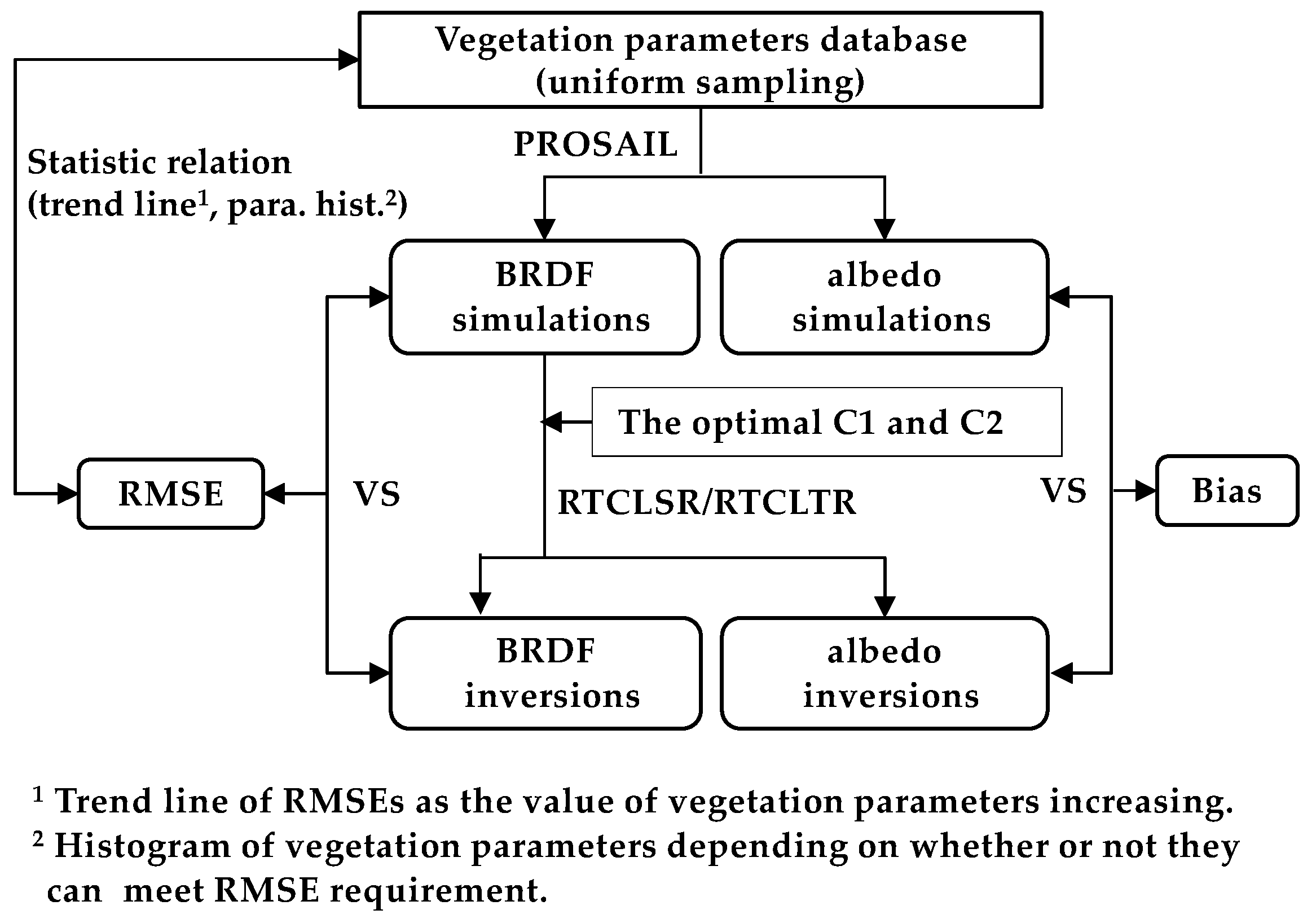
In this study, the BRF and albedo simulations derived by linking the PROSAIL model with the kernel-driven Ross-Li models are compared for the first time to examine their consistency in BRFs. First, 20,000 sets of BRFs were produced through the simulation method by the PROSAIL model, which covered various optical and structural parameters of vegetation canopies and contained 397 angles for each data set. Then, these data were input into the kernel-driven models for calculating the BRFs in the same solar and viewing geometries. The albedos were then calculated from the BRFs of both models. Finally, we compared the two models in terms of their BRFs and albedos and examined how vegetation parameters affect such a model link. To further strengthen such an investigation, 21 sets of multiangle reflectances were also used in this study. Finally, we conclude this study with a summary of the findings.

2. Methods

2.1. The Kernel-Driven BRDF Model and Anisotropy Flat Index (AFX)

The kernel-driven model derived from the Roujean model contains three adjustable coefficients that are used for optimal BRDF fitting based on directional reflectance observations [30,31,33,34,35]. This model characterizes surface reflection as a simple linear combination of three types of scattering, and the general formula is given as Equation (1).
R ( θ i , θ v , φ , λ ) = f i s o ( λ ) f v o l ( λ ) K v o l ( θ i , θ v , φ ) f g e o ( λ ) K g e o ( θ i , θ v , φ ) ,
where R is the surface directional reflectance, isotropic scattering is a constant (1.0), K v o l is the volumetric scattering kernel caused by multiple scattering within canopies, and K g e o represents the geometric-optical scattering kernel associated with single scattering among canopies. θ i , θ v , and φ are the incident zenith angle (generally referred to as the solar zenith angle (SZA)), reflected zenith angle (generally called the view zenith angle (VZA)) and relative azimuth angle, respectively. f i s o , f v o l and f g e o are the weights of the three kernels. The hotspot-revised Ross Thick-Chen (RTC) volume scattering kernel is shown in Equation (2), which is a correction of the Ross Thick model that is done by multiplying a hotspot factor with its first term [33].
K R T C = ( π / 2 ξ ) cos ξ + sin ξ cos θ v + cos θ i × ( 1 + C 1 e ξ C 2 ) π 4 ,
where C1 and C2 refer to the height and width of the hotspot, respectively, and the optimal values of the two hotspot parameters can be first determined based on the minimum root mean square error (RMSE) between hotspot observations and retrievals derived from the combined RTCLSR/RTCLTR model (given in Equation (17)) [33]. ξ is the phase angle, which can be described as follows:
cos ξ = cos θ i cos θ v + sin θ i sin θ v cos φ .
K g e o was first proposed by Roujean [31], and several subsequent versions have been developed, including the sparse canopy-assuming Li Sparse-Reciprocal (LSR) kernel [17,30,34], Li Dense Reciprocal (LDR) kernel for a dense canopy [30] and sparse-dense transition Li Transit-Reciprocal (LTR) kernel [36], as shown in Equations (4)–(13) based on a literature review [37].
K L S R = O ( θ i , θ v , t ) sec θ i sec θ v + 1 2 ( 1 + cos ξ ) sec θ v sec θ i ,
K L D R = ( 1 + cos ξ ) sec θ v sec θ i sec θ i + sec θ v O ( θ i , θ v , t ) 2 ,
O ( θ i , θ v , t ) = 1 π ( t sin t cos t ) ( sec θ i + sec θ v ) ,
cos t = h b D 2 ( tan θ i tan θ v sin φ ) sec θ i + sec θ v ,
D = tan 2 θ i + tan 2 θ v 2 tan θ i tan θ v cos φ ,
cos ξ = cos θ i cos θ v + sin θ i sin θ v cos φ ,
θ i = tan 1 ( b r tan θ i ) ,   and
θ v = tan 1 ( b r tan θ v ) .
The dimensionless relative crown height h / b and shape b / r included in Equations (7), (10) and (11) are set to values of 2 and 1, respectively, for MODIS BRDF processing [17]. The LSR and LDR models are combined to develop the LTR model and perform accurate forecasting using Equation (12). The LSR model is applied at small viewing angles, and the LDR model is used at large VZAs when the critical value of B is greater than 2 [36]. Consequently, the LTR model retains the robust fitting ability of the widely used LSR model and improves the extrapolation process at large zenith angles. Therefore, to identify the model that is ideal for model coupling, the widely used LSR model, which is used as the operational algorithm of the MODIS BRDF product, and the optimal LTR model were analyzed in this study.
K L T R = { K L S R , B 2 L L D R = 2 B K L S R , B > 2 ,
where
B = sec θ i + sec θ v O ( θ i , θ v , φ ) .
Based on Equation (1), we retrieved the three optimal kernel coefficients of multiangle observations using the least squares method, where the three coefficients were constrained to be non-negative. Then, the all-directional reflectance was calculated for any incident and reflected geometry in direct mode. Therefore, BRDF inversion was conveniently performed at custom source and view directions. Next, we obtained the black sky albedo (BSA) and white sky albedo (WSA) used for the albedo comparison in Section 3.3. These parameters are integrals over only the reflected hemisphere or bi-hemisphere and are given in Equations (14) and (15).
B S A ( θ i , λ ) = 1 π 0 2 π 0 π 2 R ( θ i , θ v , φ , λ ) sin θ v cos θ v d θ v d φ
W S A ( λ ) = 2 0 π 2 B S A ( θ i , λ ) sin θ i cos θ i d θ i
The angle index AFX, which is shown in Equation (16), was derived from kernel-driven models and has been applied to extract prior BRDF archetypes. Notably, H ker _ v o l and H ker _ g e o are the bi-hemisphere integrals of the two scattering kernels [38,39,40]. AFX was designed to effectively capture surface anisotropy, and values of AFX greater than 1.0 indicate a volume scattering-dominated bowl-like BRDF shape in the principal plane. In contrast, a dome-like BRDF shape associated with the main geometric-optical scattering will appear when the AFX is less than 1.0. The BRDF shape will be flat when the two scatterings are balanced. The index was introduced in this study to examine the potential scattering types of the PROSAIL model and their effects on model coupling.
A F X = W S A ( λ ) f i s o ( λ ) = 1 + f v o l ( λ ) f i s o ( λ ) × H ker _ v o l + f g e o ( λ ) f i s o ( λ ) × H ker _ g e o
The RMSE and weight of determination ( W o D ) are generally used as evaluation criteria for kernel-driven models and are defined in Equations (17) and (18). In Equation (17), R o b s and R m o d e l refer to n observations and retrieved values. Roman et al. analyzed the retrieval accuracies of airborne and satellite observations at several spatial scales (30 m–500 m) for many land cover types and found that the average RMSEs of the RTLSR model were 0.01, 0.02, 0.05 and 0.04 in the 0.472-nm, 0.682-nm, 0.870-nm, and 1219-nm bands, respectively [41]. W o D describes the amplification of noise from observations to inversion for angle sampling, as shown in Equation (18), where K and U are the kernel matrix and its weight vector, respectively [16,35]. The noise amplification of reflectance and albedo retrieval at given angles are included in U . Generally, three quality classes are established (0–0.75, 0.75–1.25 and >2), and a W o D value less than one indicates less noise in the inversion process than in the original measurements.
R M S E = j = 1 n ( R o b s R m o d e l ) 2 n 3
W o D = [ U ] T [ ( K T K ) 1 ] [ U ]

2.2. PROSAIL Canopy Reflectance Model

The PROSAIL model is a mature canopy radiation transfer model with the advantages of simplicity, robustness, and extensive validation. The latest 4SAIL canopy model considers hotspot effects, and the PROSPECT-5 model, which describes leaf optical reflectance and transmittance, is referenced in this study [6,7,14]. Additionally, simulation generation is a critical application for the PROSAIL model, and it can be in favor of the examination of the links among all the variables in the radiative transfer process [2].
At the leaf scale, the PROSPECT model can simulate directional-hemispherical reflectance and transmittance from 400 nm to 2500 nm for monocotyledonous, dicotyledonous and aging leaves [42]. Considering the rough surfaces of leaves, this model uses the maximum incident angle α to represent the diffused features. Meanwhile, an internal leaf is assumed to be composed of N parallel homogeneous layers. Reflectance and transmittance are calculated based on Equations (19) and (20), where ρ 90 and τ 90 denote the reflectance and transmittance of every internal layer, and R N 1 , 90 and T N 1 , 90 are the total reflectance and transmittance of the internal N-1 layers, respectively. Finally, the PROSPECT model can be simplified to include only the plate transmission coefficient θ and the absorption coefficient k , which are given in Equations (21) and (22), where k is related to the absorption K i of biochemistry component i , its weight C i and the absorption of albino leaf k e before 500 nm.
ρ l ( λ ) = R N , α = ρ α + τ α τ 90 R N 1 , 90 1 ρ 90 R N 1 , 90
τ l ( λ ) = T N , α = τ α T N 1 , 90 1 ρ 90 R N 1 , 90
θ ( 1 k ) e k k 2 k x 1 e x d x = 0
k ( λ ) = k e ( λ ) + i C i K i ( λ ) N
The SAIL model is one of the earliest CR models based on the four-flux theory with 4 up- and down-scattering and absorption fluxes that are assumed for homogeneous, horizontal and infinitely extended vertical leaf layers [29]. The modified 4SAIL model is numerically robust and speed optimized, as given in Equation (23) [3].
ρ c ( λ ) = 4 S A I L ( L A I , A L A , ρ l ( λ ) , τ l ( λ ) , P s o i l ( λ ) , S Z A , V Z A , φ , H s p o t , S K Y L ) ,
where ρ c is the canopy reflectance, which couples ρ l and τ l from the PROSPECT model. Other input parameters are shown in Table 1, and the reasonable ranges of parameters are based on previous studies of model intercomparison and sensitivity analysis [43,44]. Considering all the parameters, the extinction and scattering of the radiant flux of each leaf layer from the bottom to top of the canopy can be obtained, and CR can be calculated based on the cumulative energy transition.

2.3. Data and Experimental Design

Experimental design is the foundation of model comparison, and the overall design is shown in Figure 1. Almost all possible canopies simulated by the PROSAIL model can be considered via numerous simulations. In total, 20,000 vegetation parameter combinations were generated using the Saltelli periodic function [45] by the uniform sampling of nine leaf and canopy parameters over the ranges that are shown in Table 1 with reference to the experimental designs of previous studies [43,44], except for Cbrown and SKYL. Considering that most leaves do not contain brown pigment [43] and the intrinsic BRDF is not necessarily related to the component of diffuse irradiance [46], the two remaining parameters were set to zero. Subsequently, the parameters were randomly combined to ensure diverse canopies. Then, we calculated the corresponding directional reflectances and albedos by direct simulation using the PROSAIL model in the red band (659 nm) and near-infrared (NIR) band (865 nm), where the angle distribution reflects the general geometry in remote sensing observations [47]. The intervals were 15°, 10° and 30° for the SZA (0–60°), VZA (0–80°) and φ (0–330°) with a total angle number of 397, respectively, based on typical angle ranges and experimental design [47,48]. POLDER can yield directional reflectance when SZA and VZA are close to 70° [49], and VZA ranges from nadir to 75° off-nadir for the airborne Cloud Absorption Radiometer (CAR) data set and MODIS satellite [33,41]. In addition, we set the maximum VZA to 80° for robust inversion ability, even at large angles close to 90° [17]. A W o D of 0.0027 was observed, which indicated a good angle distribution with negligible noise, as discussed in Section 2.1.
As observations, the directional reflectances obtained from the PROSAIL model were then input into the kernel-driven RTCLSR/RTCLTR model to reconstruct the reflectance anisotropy. First, for the two adjustable hotspot factors C1 and C2 in the RTC model, the optimal values corresponding to the minimum RMSE of hotspot observations in each data set were determined [33]. Then, the optimal C1 and C2 factors were applied to the RTCLSR/RTCLTR model to retrieve the three kernel coefficients based on the database of 20,000 directional reflectances discussed in Section 2.1. There were 5390 and 1092 sets of data in the red and NIR bands, for which the volumetric scattering kernels were zero without hotspot effects. Subsequently, reflectances at the simulated angles and albedos (BSA at the five SZAs and WSA) were inverted based on the forward algorithm of the RTCLSR/RTCLTR model. Finally, we compared the directional reflectances and albedos of the two models based on the RMSE and bias. Notably, we called the comparison of directional reflectances “BRDF comparison” because the simulated data set of directional reflectance captured the main BRDF effects, which benefited from sufficient sampling at multiple angles. Before the comprehensive comparison, BRDF and albedo consistency was preliminarily examined for a typical canopy, and the BRDF effect was compared in the viewing hemisphere and principal plane. Additionally, we determined the reasons for model discrepancies by conducting statistical analyses based on vegetation parameters and RMSEs, including trend line and parameter distribution analyses based on whether error requirements were met, as noted in Section 2.1.
To further analyze the BRDF consistency of linking the two models, 21 sets of multiangle reflectances capturing a wide range of forest-grass-crop vegetation types were collected, where the LAI measurements were inferred from an LAI-2000 instrument. Most of these datasets are from PARABOLA radiometer measurements in the First International Satellite Land Surface Climatology Project (ISLSCP) Field Experiment (FIFE) [50], and the remaining data are from radiometer measurements by Kimes and Ranson [51,52,53]. The datasets were collected under nearly clear-sky conditions and have been widely used in the validation of the kernel-driven model [54,55,56] as well as extracting BRDF prior knowledge [40]. The central wavelength is 662 nm and 826 nm from PARABOLA radiometer from data 6 to data 18. For the remaining 8 sets of data that did not describe their central wavelength, we still used the 659 nm and 865 nm for PROSAIL simulation. There are 6801 BRF samplings altogether in which the VZA varies from 0 to 80°, and the SZA ranges from 16° to 82° with a total number of 126. Their detailed information is shown in Table 2, and the SKYLs for the remainder of the data were determined based on the observation of data 7 (SKYL varies with SZA and band), 16 and 17 (average SKYL), except for the first five groups which had been corrected based on the simulated diffuse fraction [53]. In addition, the Ns of some data were given based on vegetation classification and their fraction of dead leaves [57], and ρ l and τ l for data 1 and 5 as well as ρ c for data 1 and 4 were observed. Because of the lack of vegetation measurements in these early campaigns, the other eight input parameters of the PROSAIL model were determined by looking for the optimal BRF fitting compared to the observations from the 20,000-parameter database mentioned above. Leaf inclination of the typical canopies for corn and soybean (data 1 and 5) presented a random distribution all over the range of φ [53], so we did not limit the scope of ALA during the parameter matching. Detailed information can be found in the footer of Table 2. Finally, we evaluated the two models based on their simulated or retrieved BRFs in comparison with the reflectance observations, and the resulting albedos were used for the cross-comparison.

3. Results

3.1. A Case Study for a Typical Canopy

In this section, we first provide an extreme example to parameterize a typical canopy as given in Table 1. The reflectance in the viewing hemisphere and principal plane that exhibits the most significant BRDF effect with SZA = 30° as well as the albedo, are shown in Figure 2. The polar plots have a common scale ranging from the minimum to the maximum for each row. The dome-shaped BRDF indicates that surface scattering is more obvious in the red band (Figure 2f), while volume scattering dominates in the NIR band, leading to a bowl-shaped BRDF (Figure 2i). The significant difference in scattering type is caused by high chlorophyll absorption in the red band and high leaf transmission in the NIR band, which lead to dominant single and multiple scattering effects, respectively. A slight overestimate can be seen in the forward direction, whereas backward scattering is slightly underestimated. This pattern is closely related to the solar principal plane because reflectance anisotropy is most significant in the principal plane, and discrepancies between models are easier to observe [31]. The hotspot-fits are somewhat better for the RTCLSR model than for the RTCLTR model, which demonstrates that the hotspot-corrected RossThick kernel (i.e., KRTC) plays a better role in conjunction with the LSR kernel than the LTR kernel [30,36] in this case. The inconsistency can also be seen at large view angles in the red band, which shows that the RTCLTR model presents better fits than the RTCLSR model because the derivation of the LTR kernel includes the mutual shadowing effect [37,40]. These two models are highly consistent in the NIR band.
Figure 2d,e,g,h imply that bias between the kernel-driven model and PROSAIL models for the entire viewing hemisphere is less than 0.01 and 0.04 in the two bands. In addition, the absolute and relative RMSE of reflectances at 397 sampling angles between the two kinds of models are 0.0020 (1.10%, red, RTCLSR), 0.0017 (0.96%, red, RTCLTR), 0.0185 (2.53%, NIR, RTCLSR) and 0.0184 (2.53%, NIR, RTCLTR), respectively. Smaller RMSEs are found for the entire hemisphere with the statistic of 0.0012 (0.68%), 0.0010 (0.57%), 0.0082 (1.12%) and 0.0080 (1.10%). Notably, a significant difference can be seen at large relative azimuth angles especially for the NIR band, which may be related to the assumption of leaf distribution in the two models. There is an asymmetric BRDF shape along the principal plane due to the random leaf azimuth distribution for the PROSAIL model [29], whereas a symmetric shape is assumed in the kernel-driven model. In addition, a somewhat low-level accuracy at large angles for the semi-empirical Ross-Li model also contributes to such discrepancies [30,31]. Such a comparison for a typical example demonstrates that the BRFs by linking these two models are not necessarily consistent although the consistency between them is dominant.
The variability in BSA is similar to that of the BRFs, with a high value from the PROSAIL simulation when the SZA is greater than 40° and low values at smaller view angles (Figure 2). Notably, the largest deviations can arrive at 0.004 and 0.075 at 89° in the two bands. Despite these discrepancies, WSA exhibits good agreement between models, as shown in Figure 2. This result shows that once these two models are linked to evaluate the potentials in retrievals of biophysical/structural parameters using a simulation method, such a divergence between models should also be appropriately considered, although a generally good consistency exists between PROSAIL-generated BRFs and the fitting results by selecting an apt kernel-driven BRDF model.

3.2. General Consistency in BRFs between the Two Models

3.2.1. Comparison of Directional Reflectance Based on the Fit-RMSE and AFX Statistics

Using 20,000 sets of BRF simulations generated by the PROSAIL model that cover the main variations of the inputs from various biophysical/structural variables (Table 1), the comparison of BRFs between the RTCLSR and PROSAIL models is shown in Figure 3. The results of the RTCLTR model are generally similar to those of the RTCLSR model, so the results are not presented due to space limitations. Scatter plots are used to illustrate how the correlations are shown between the two models. The scatter plots are sliced into five equal-density levels in terms of the reflectance magnitude from 1 (maximum) to 5 (minimum) with the interval of 0.01 (Figure 3a,b). Figure 3a,b shows that the total R2 is greater than 0.92, with negligible biases in the red and NIR bands, indicating that the two models are generally in good agreement for various canopies. 80% of the BRFs with density levels from 1 to 4 fall within the tolerance range although a few errors reach 0.11 and 0.17 in the two bands, as shown in Figure 3c and Table 3. Furthermore, 88.6% of the 20,000 fit-RMSEs are less than 0.02 in the red band, and 79.0% of canopies are within the tolerance range of 0.05 in the NIR band (Figure 3c). The total RMSEs are 0.0131 and 0.0436 (Figure 3a,b), with average fit-RMSEs of 0.0092 and 0.0355 in the two bands, respectively, as shown in Table 3.
The hemispherical distribution of average biases for the 20,000 sets of BRFs between the two models is calculated, where the angular bins refer to the BRDF sampling in Figure 1b and two of the SZAs that are shown in Figure 3d–i. When the SZA is within 30°, a slight underestimation of the PROSAIL-simulated hotspot BRFs by kernel-driven models can be found in the red band. As the SZA increases from 0° to 60°, model discrepancies tend to occur in large view zenith angles, and an obvious overestimation of the PROSAIL simulation BRFs by the kernel-driven BRDF model appears at the largest 80° VZA and 330° φ of the angle sampling. For the red band, the bias at large view zenith angles for the RTCLTR model is more significant than the result of the RTCLSR model (i.e., Figure 3d,e) except for the SZA of 60°, where fewer discrepancies are found for the RTCLTR model (Figure 3f,g). Unlike the red band, the presentation of model discrepancy between the PROSAIL model and the two kernel-driven models is generally similar in the NIR band. All results show that there is a general consistency in BRFs between these two models; however, few discrepancies in BRFs between two models mainly arise from hotspot direction and larger view zenith angles, somewhat depending on the variation of solar zenith angle. The RTCLTR model performs similarly in fitting these simulation BRFs generated by the PROSAIL model, although fitting results are somewhat better in a large view zenith angle (e.g., VZA > 65°). This result is generally consistent with the result examined in the case study in Section 3.1.
The AFX was applied to examine the scattering types among diverse canopies simulated from the PROSAIL model, as shown in Table 3 and Figure 4a. The AFX approximately satisfies the normal distribution clustered near 0.85 in the red band and the skewed distribution clustered at 0.95 in the NIR band (Figure 4a). To analyze the main BRDF properties in the two bands, 1.0 was taken as the critical value of AFX based on its characteristic [40]. Notably, 91.7% of AFXs are less than 1.0 in the red band, and the average value is 0.85, which implies that geometric-optical scattering is dominant. However, the numbers of data points are almost equal on either side of 1.0 and concentrated at approximately 0.95 when AFX is less than 1.0 in the NIR band. Additionally, the average value is 1.05. These results indicate primary isotropic scattering and volumetric scattering. Moreover, the range of AFX in the red band is wider than that in the NIR band, which is consistent with MODIS but over a narrower range [38,39,40]. The leading type of scattering in each band is related to high chlorophyll absorption in the red band and high leaf transmission in the NIR band, as discussed in Section 3.1. These factors strengthen single and multiple scattering. As a result, different scattering characteristics are observed for the two bands, and these characteristics indicate that the red band can capture more variability in the surface reflectance anisotropy than can the NIR band. The dominant volumetric scattering in the NIR band is theoretically caused by the multiple scattering of foliage leaves within canopies in the PROSAIL model. Furthermore, AFX variation has no significant impact on fit-RMSE in the red band (Figure 4b), while the RMSEs tend to increase as AFX increases in the NIR band (Figure 4c). This indicates that these models should be cautiously combined over canopies that represent extreme volume scattering effect (large AFX values), as is generally characterized by a dramatic BRDF shape, especially in the NIR band [40].

3.2.2. Model Discrepancies regarding Vegetation Parameters

To further explore the reason for the discrepancies of linking the RTCLSR and PROSAIL models, we examined the relationships between BRDF fit-RMSE of the two models and nine biophysical and background vegetation parameters. Figure 5a–f shows that the LAI and ALA can affect the RMSE in both the red and NIR bands and that C a b and P s o i l can affect the RMSE in the red band, all of which are sensitive parameters to CR [43,44]. Except for the sensitivity of fit-RMSE to the four input parameters of the PROSAIL model, other canopy structures exhibit subtle variations in RMSE throughout their ranges.
First, LAI is a critical factor that contributes to CR [23], and model discrepancies vary with LAI values. For a sparse or small-leaf canopy (LAI ≤ 1.0), RMSE exhibits an upward tendency, followed by a downward trend (LAI > 1.0) in the red band, as shown in Figure 5a, and a slight increase in the NIR band, as shown in Figure 5e. Meanwhile, large RMSEs are obtained when the LAI is less than 1.0 (Figure 5g). In contrast, as the LAI increases, the RMSE in the NIR band becomes more stable (Figure 5k). Notably, a relatively significant correlation can be found only for small LAIs in the NIR band, where R2 is 0.2600. Consequently, model coupling is more applicable to low-density leaf or sparse canopies in the NIR band, whereas high-density leaf or dense canopies can be analyzed using the red band. These differences in relation to the LAI range may be associated with the different sensitivities of the LAI to CR. Notably, significant sensitivity can be observed at small LAIs in the two bands, while large LAIs are only sensitive in the NIR band [43,44].
Another essential canopy parameter is ALA, which is sensitive to CR in the NIR band [43,44] and displays similar tendencies in the two bands. Nevertheless, the fit-RMSE increases more significantly at large leaf angles in the NIR band, where R2 is 0.5298, than in the red band (Figure 5b,f), and all the RMSEs that exceed 0.05 are associated with large ALAs (ALA > 60°) (Figure 5l). In addition, large ALAs also induce greater error in the red band (Figure 5b,h). Therefore, the kernel-driven model and PROSAIL model should be cautiously linked for vegetation estimation at large ALAs (mainly erectophile canopies), especially for the NIR band.
Contrary to the LAI, the fit-RMSE appears to decline at low-density leaf component C a b values and then levels off as C a b increases (Figure 5c). Simultaneously, the aggregation of large errors can be observed when C a b is less than 20 μg/cm2 (Figure 5i). As a result, small C a b values are not a reasonable choice for the joint model.
The final parameter that contributes to the discrepancy between the kernel-driven model and PROSAIL model is P s o i l . A subtle increase can be observed when the background soil becomes brighter, and consequently, most large errors accumulate when the soil exhibits high brightness. Therefore, in future studies, we should not focus on vegetation growing on bright soil, such as saline land, and should instead perform experiments on black soil.

3.3. General Consistency in Albedos between the Two Models

Land surface albedo is an essential factor in energy balance, as introduced in Section 2.1, and an absolute accuracy of 0.02~0.05 is usually required in many applications [58,59]. The GCOS report of 2016 (GCOS 2016) proposed the requirement that the absolute error of 0.0025 or relative deviation of 5% should be achieved within the next 10 years [60]. Additionally, land surface albedo is one of the main inversion parameters of the kernel-driven model, which is the integral of directional reflectance and can reflect the energy transfer. Therefore, we examined the consistency of linking the two models to provide some advice regarding albedo estimation. In this section, we do not show the results of the RTCLTR model because they exhibit little difference from those of the RTCLSR model. Despite the discrepancies in directional reflectance, Figure 6 shows good overall agreement between WSA and BSA at the 5 SZAs of simulations with R2 values greater than 0.98 in the red and NIR bands. Moreover, less discrepancy is found in the WSA than in the BSA. Notably, a subtle overestimate of WSA is shown by the red band, whereas slight underestimates are found for the total BSA in both bands and for the WSA in the NIR band. Furthermore, the RMSEs of WSA between the two models are 0.0029 and 0.0156 in the two bands, which are within the relevant precision range. Although a wider range of AFX change is found in the red band, WSA and BSA exhibit better agreement in the red band than in the NIR band, which is consistent with the directional reflectance results in Figure 3a.
To assess the contribution of the SZA to the BSA in detail, the percentages of the albedo deviations in six ranges were calculated, as shown in Table 4 and Figure 6c,f. Figure 6c,f clearly shows that most of the albedo deviations are less than 0.02 between these two models (red and blue areas), especially for the red band. However, some extreme errors ( | d e v i a t i o n | > 0.05) can be observed, particularly for the BSA when the SZA is 0° or 15° in the NIR band. The BSA varies greatly as the SZA changes, exhibiting the most similar error distribution to that of WSA at 60°, among the five SZAs tested. The transition from underestimation to overestimation can be clearly observed as the SZA increases, and this change is in agreement with the finding that the BSA exhibits an increasing trend as the SZA increases (Figure 2) [14]. This phenomenon is more obvious in the red band, and the largest difference is observed when the SZA is at nadir. Extremely high consistency is found at the turning point, at which almost all the canopies meet the 0.02 tolerance threshold.
Overall, the percentages of deviations less than 0.02 are 99.98% (WSA) and 98.65% (total BSA) in the red band and 97.99% and 86.51% in the NIR band. For a tolerance of 0.05, the percentages reach 99.99% and 99.97 in the red band, whereas 1.11% and 3.73%, respectively, of the canopies do not exhibit good agreement in the NIR band. In addition, the total relative deviations of WSA are 5.74% and 1.04% in the red and NIR bands, which can basically meet the requirement of GCOS 2016. We analyzed the reason given rise to these outliers especially for WSA in the NIR band (Figure 6d), where we found that the two sensitive parameters of LAI and ALA have a similar effect on WSA consistency compared to the result of reflectance in Figure 5e,f. In addition, little content of Cm seems to cause a larger difference. The good consistency in terms of the WSA may be explained by the compensatory effects of the BSA at different SZAs, which cause dramatic variance in the estimation accuracy as the SZA changes. Despite some extreme changes in the directional reflectance, the albedo is highly consistent, especially for the WSA, between the RTCLSR inversion and PROSAIL simulation results. Therefore, further research on albedo can be performed by coupling the two models and assessing their estimations.

3.4. Consistency in BRFs and Albedos between the Two Models Based on Field Observations

Similar to the comparison for the 20,000 PROSAIL simulation, the comparison of the simulated (PROSAIL) and retrieved (RTLSR) BRFs and albedos were also implemented based on 21 sets of BRF observations as shown in Figure 7, which is helpful in further exploring the BRDF consistency. For all the 6801 BRFs (Figure 7a–d), there is good agreement overall with the observation results. In addition, a better fitting of BRF observations for the RTLSR model can be seen than PROSAIL simulations in the red and NIR bands, which may be related to the uncertainty caused by vegetation parameter matching. Additionally, we preliminarily explored the relationship between angle index AFX and model error for each set of data (Figure 7e), from which we can see that the absolute biases between RTLSR retrievals and observations for all 21 data are close to the zero line with values less than 0.002, as well as in Figure 7f,g. Notably, bias presents a downward trend as AFX increases in the NIR band for PROSAIL simulations, which is inconsistent with the result of the 20,000 PROSAIL simulations (Figure 4c); therefore the influence of the AFX on model must still be investigated. In total, there are 14 sets of data where the absolute values of bias are less than 0.02 in the red band, and results for 12 sets of data are less than 0.05 in the NIR band for the PROSAIL simulations. For fit-RMSEs, the number is 19 and 14 in the two bands for RTLSR models, whereas smaller numbers are observed for the PROSAIL simulations, which are 7 and 5. The uncertainty from BRF measurements contribute to the model discrepancies, where each dataset was collected in a period by assuming a stable land surface [52]. The better fitting result from Ross-Li model is related to the extra error introduced by parameter matching of the PROSAIL model. In addition, the semi-empirical RTLSR model can be more flexible to fit the observations by the interpolation (or extrapolation) method than the physically-based PROSAIL model [56,61].
In terms of the relationship between the vegetation parameter and model discrepancy, similar patterns of fitting-error with the change of vegetation parameters are observed compared to Figure 5; this excludes soil reflectance, which seems to show no change. Bias between the PROSAIL simulation and observations is significant when LAI is less than 2.0 in the red band as shown in Figure 7f, which agrees with the results (Figure 5a). Nevertheless, the result for LAI is inconsistent in the NIR band (Figure 5e). In addition, bias is smaller when ALA is less than 30°, whereas larger bias is observed when ALA is greater than 50° in Figure 7f, which matches the early results well (Figure 5b,f). The statistics of average error for the four parameters mentioned in Figure 5 are shown in Table 5, where it is apparent that most of the error distribution is consistent with the results from the 20,000 sets of PROSAIL simulations in Figure 5. For a few of data that have a different trend with the results in Figure 5, these discrepancies may be due to the uncertainty mentioned above.
Finally, we inter-compared the albedo retrievals for the two models due to the lack of true values, including WSA and BSA at the 126 observed SZAs. As a whole, the values of WSA for RTLSR retrievals are lower than those of the PROSAIL simulations in the red band, whereas a better agreement is observed in the NIR band. For the fitting-error, all the R2 values are greater than 0.76, and the total RMSE is 0.0212 and 0.0545 (with the relative deviation of 24.00% and 5.67%) for WSA in the two bands. In addition, there is a smaller RMSE for BSA. The albedo consistency for the 21 sets of observations is not as good as the result of the 20,000 sets of PROSAIL simulations, which may be caused by the uncertainty from BRF measurements and parameter matching as mentioned in the analysis for BRFs. In addition, the two models show a relatively good consistency without the effect of external uncertainty as shown in Figure 6, which confirms that these uncertainties are probably the major source that causes the somewhat large RMSE in Figure 8. In general, the two models have a generally good consistency in matching BRFs and albedos.

4. Discussion

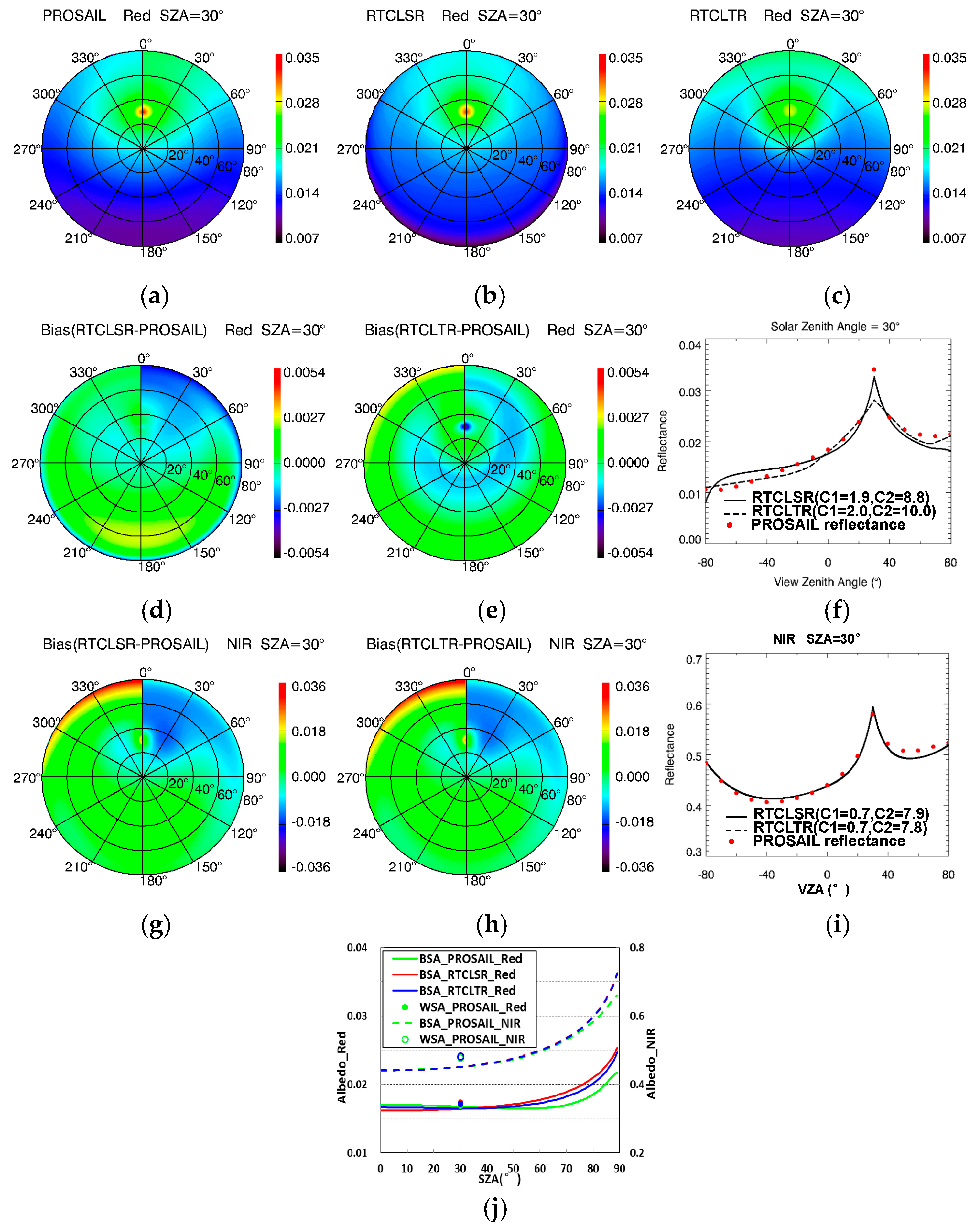
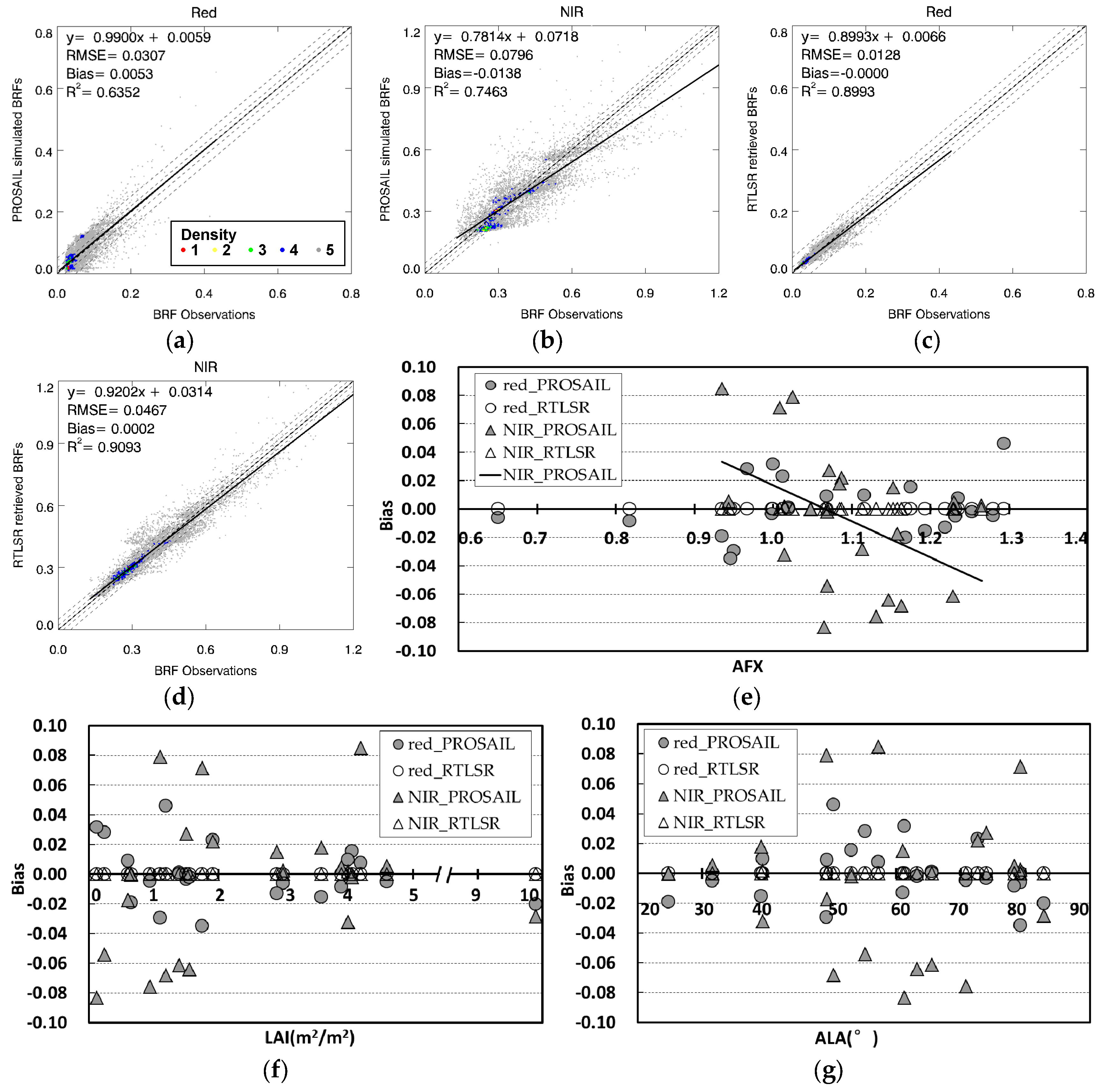
In this study, the directional reflectance and albedo results of PROSAIL simulations as well as a variety of types of observations and their inversions using the hotspot-revised RTCLSR/RTCLTR model were compared for the first time, and good global agreement was observed, despite a few extreme discrepancies. The AFX was utilized to explore the scattering types among diverse canopies of PROSAIL simulations. Furthermore, the sensitivity of the model consistency to the vegetation structure was investigated to obtain a better understanding of the model linking. Additionally, the albedo, which is an essential factor in the models, was considered for further comparison to offer advice regarding albedo inversion by combining the two models.
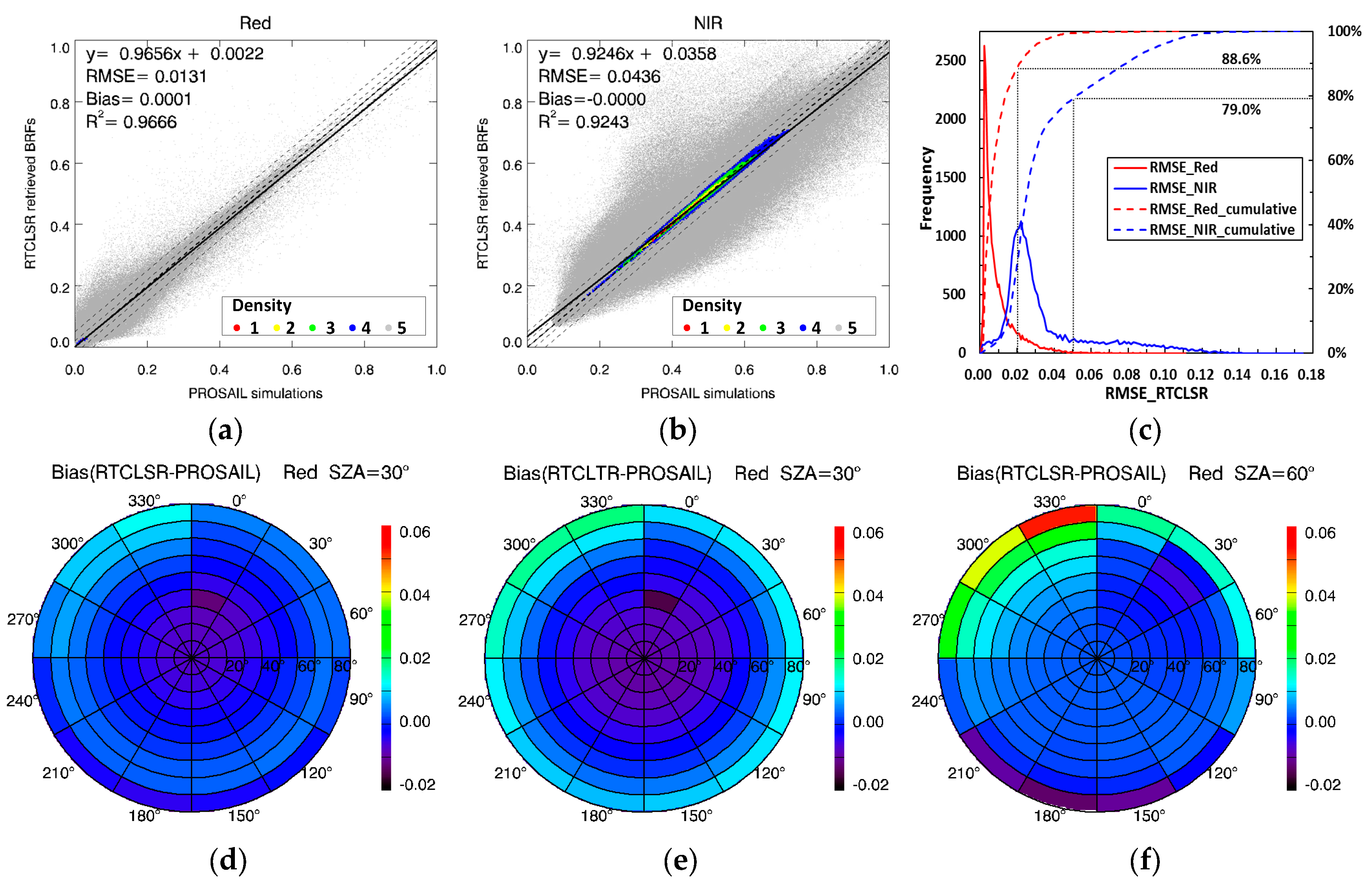
The generally similar BRDF results of the RTCLSR model and the optimal RTCLTR model may be due to the robustness of the MODIS operational LSR model. Therefore, the commonly used RTCLSR model can be used in future model coupling. The case study results involving a common canopy exhibited good overall agreement, indicating that model coupling can be performed when only typical vegetation is considered. Despite the extreme error in the directional reflectance (Figure 3), 88.6% and 79.0% of canopies can meet tolerances of 0.02 and 0.05 in the red and NIR bands, respectively. On one hand, the kernel-driven model has proven to be reliable for various canopies [56,62,63], and therefore such a consistency is not surprising. On the other hand, however, discrepancies between these two models remain and may be caused by the differences in model theory, as discussed in the introduction. In addition, the diverse combinations of vegetation parameters required to cover complete canopies may be responsible for these differences because unreasonable combinations that do not exist in the real world may be included. However, no better way of performing a complete analysis has been developed to date, and the method of random combination has been widely applied in comprehensive analyses [43,44]. Therefore, further studies of the interactions among vegetation variables are necessary to guide the experimental design. Nonetheless, we have obtained an overall understanding of the consistency between the two models within the capacity of the PROSAIL model, and these findings will facilitate further studies on joining these two models. In terms of the field measurements, the RTLSR model presents better fitting compared to the PROSAIL model, which may imply that the semi-empirical kernel-driven models have more potentials in flexibly fitting actual multiangle observations than the physical models that require the parameterization of various biophysical/structural and spectral variables as inputs. In addition, more discrepancies were observed in the result for the field data than that of the 20,000 simulations, which may be related to the uncertainties during the BRF measurements and vegetation parameter matching.
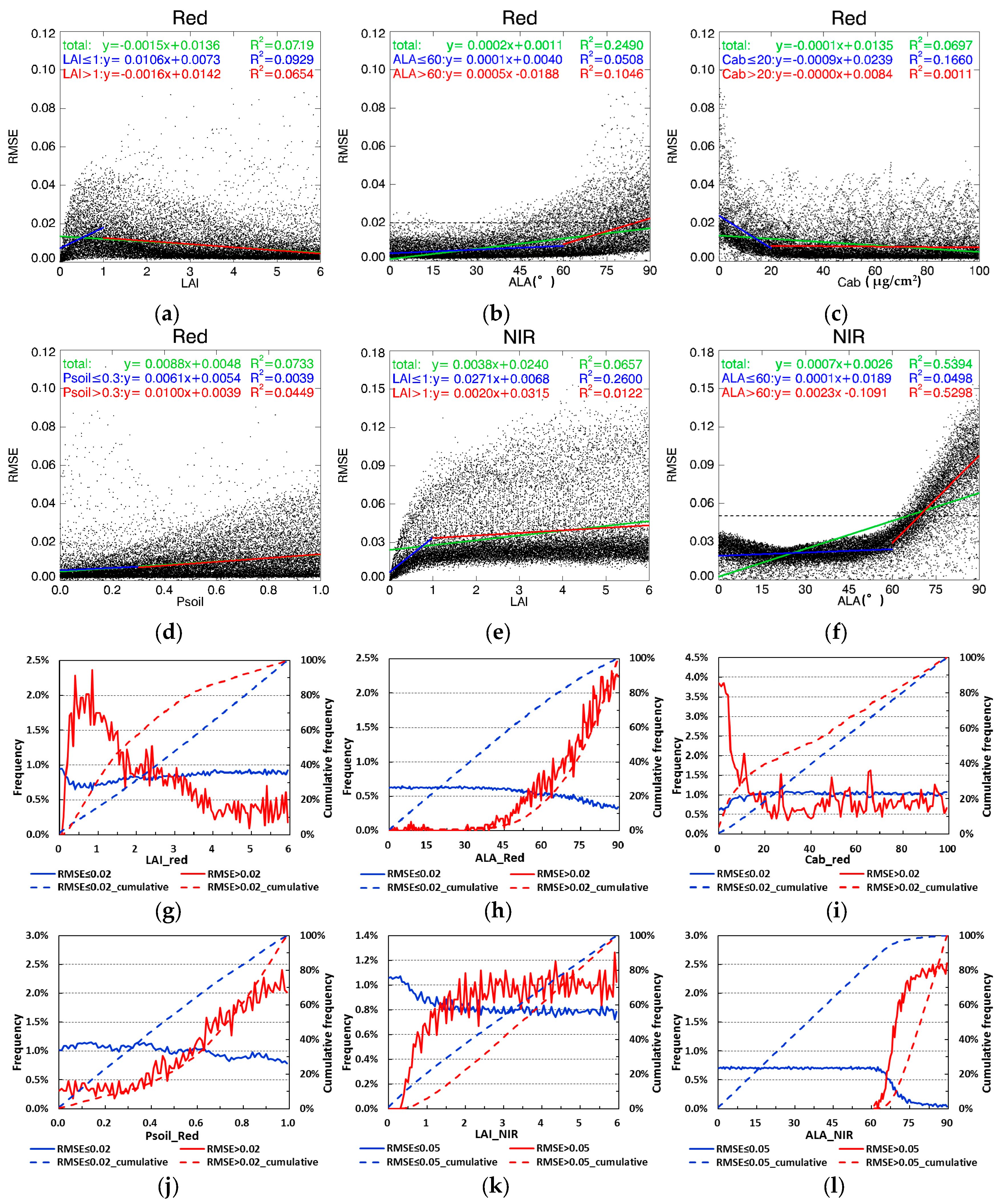
To further explore the reasons underlying these discrepancies, the links between the vegetation structure and model differences were analyzed in detail, and canopy parameters, including LAI, ALA and P s o i l , were shown to be sensitive in the red band. Similarly, LAI and ALA can also affect the fit-RMSE in the NIR band. At the leaf level, variations can only be observed as C a b changes. This result suggests that the largest effect on model discrepancy occurs at the canopy level, especially for ALA, and that the canopy structure can significantly affect reflectance in the red and NIR bands, as shown in previous studies [1]. Because of the equal variation derived from the uniform sampling of every parameter, the sensitivity analysis can be considered reliable. Hence, the analyses of canopies with small LAI and Cab values and those with large ALA and P s o i l values suggest that we should be cautious when combining the two models in the red band and that further examination is required for both large LAIs and erectophile canopies in the NIR band. Notably, a real vertical leaf is limited [29]. This limitation may affect the validation of PROSAIL model simulations and, subsequently, comparisons such as those performed in this study. Moreover, large ALAs (erectophile canopy) generally cause a dramatic change in the BRDF shape [29], for which a large hotspot is generally observed. Our group is working on a hotspot correction for the geometric-optical scattering kernel, and a reexamination of these discrepancies is likely necessary using the updated model.
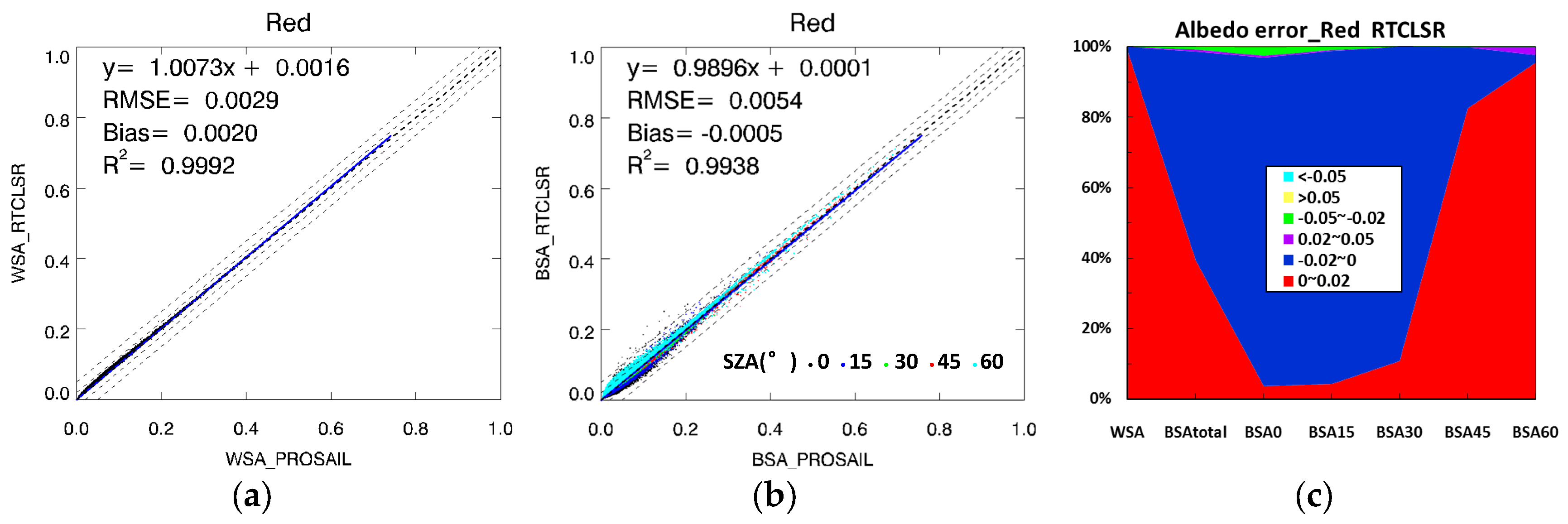
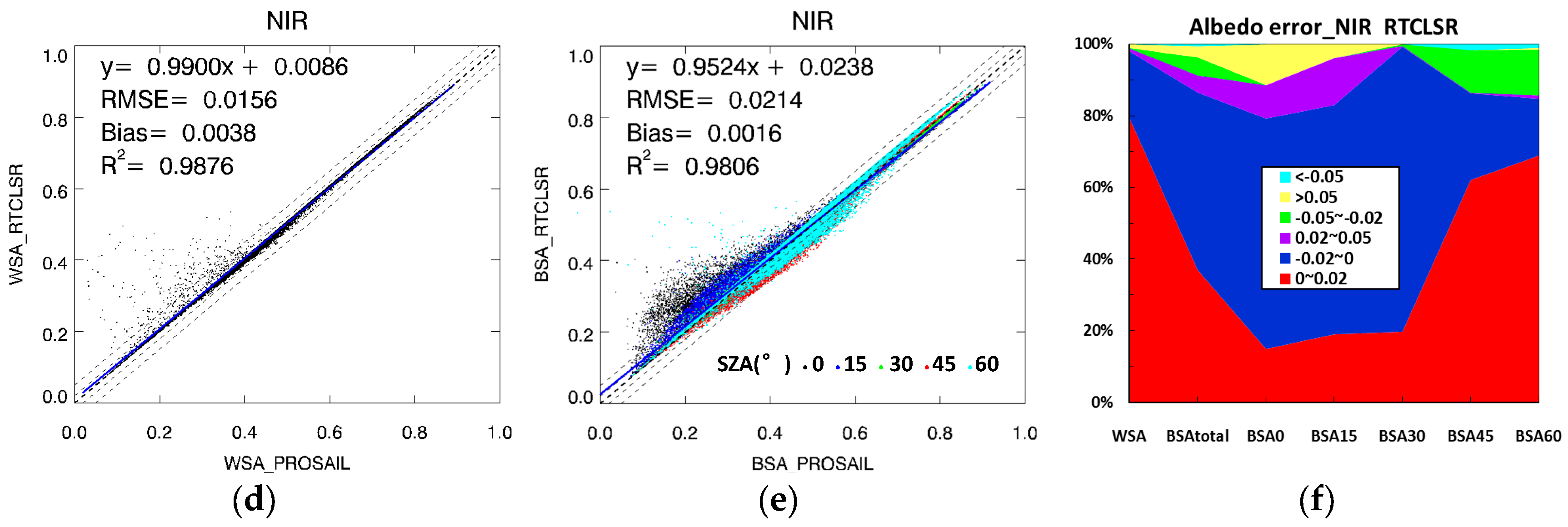
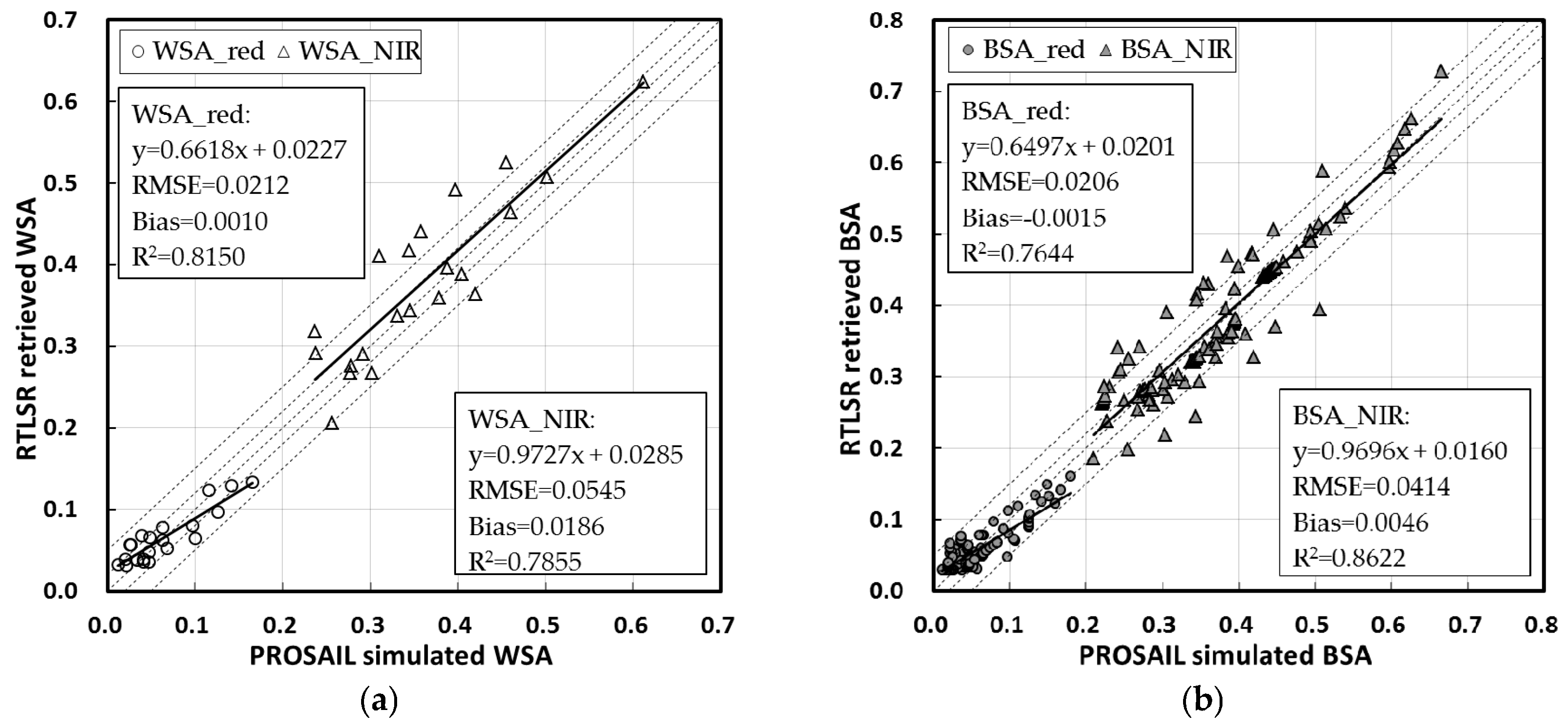
Parameter inversion is a potential application of linking these two models. The two models used in this study benefit from both the complete description of the vegetation structure in the PROSAIL model and the robust BRDF simulation and inversion of the kernel-driven model. In this study, we examined the parameter consistency in terms of albedo as an example. The highly consistent albedo reflects reliable model coupling for estimation and evaluation. Limited to the five SZAs used for BSA comparison, the BSA consistency must be further examined for other SZAs. Similarly, good consistency was observed for the 21 sets of field BRDF observations, in which the lower agreement may be due to error that occurs during the post-processing of the vegetation parameter matching and the uncertainty of from BRF measurements themselves. Based on the parameter matching, the retrieved and measured LAIs were compared. The result shows good consistency with a high R2 of 0.8584 and a total RMSE of 0.95, which can probably meet the precision of current LAI products (around ±1.0) from MODIS and CYCLOPES sensors [64]. Such an attempt for the LAI retrieval may initially demonstrates the feasibility of PROSAIL inversion by linking the two models. The three coefficients f i s o , f v o l and f g e o included in the MODIS BRDF product are promising for estimating vegetation parameters, such as in the CI [25,26] and canopy height [28], as discussed in the introduction. In addition, the AFX has been applied to extract prior BRDF archetypes and can capture the main BRDF variety, which is potentially related to the vegetation architecture [38,39,40]. Thus, these BRDF factors could be added as constraints for parameter retrieval using the PROSAIL model in the future, where the relationships between these BRDF parameters and the vegetation structure can be further studied. Notably, the model consistency analysis in this study provides meaningful guidance for such studies. We preliminarily analyzed the sensitivity of retrieved Ross-Li model coefficients against PROSAIL parameters by using the Extended Fourier amplitude sensitivity test (EFAST) method. The result is consistent with Figure 5, which suggests that sensitive parameters on BRDF effect occurs at the canopy level, especially for the ALA. Additionally, real data, such as sufficient measurements of LAI and ALA as well as other vegetation parameters, can be used to verify the results of these comparisons during their estimations. The strategy of comparison of BRDF for linking different models proposed in this study is still applicable for many other physical BRDF models beyond the PROSAIL model, and it would be promising to estimate various vegetation structure related to the physical models from satellite BRDF data by considering the BRDF consistency of model linking.

5. Conclusions

In this study, the potential in linking two widely used models (i.e., a semi-empirical, hotspot-revised, kernel-driven model, including the RTCLSR and RTCLTR models, and the physical PROSAIL model) was comprehensively investigated in terms of BRDF and albedo. A typical canopy was first exemplified in the comparison in viewing hemispherical and principal planes to examine the potential in linking the two models. In total, 20,000 sets of parameter combinations were applied in a comprehensive analysis based on the PROSAIL model and were used to generate the PROSAIL multiangle reflectance and albedo. Then, BRDF and albedo values were obtained using the kernel-driven model. Finally, the reflectance and albedo values of the two models were compared, and the correlations between vegetation parameters and model discrepancy were further explored. To further strengthen the investigation, 21 sets of field BRDF observations that cover a variety of land surface classes were also introduced into the study.
Overall, similar results were observed for the RTCLTR and RTCLSR models. This finding indicates that the MODIS operational LSR model provides a robust inversion technique, although the LTR model is considered to be the optimal version of the LSR model [36]. Globally, the two models agree well in terms of directional reflectance for diverse canopies (R
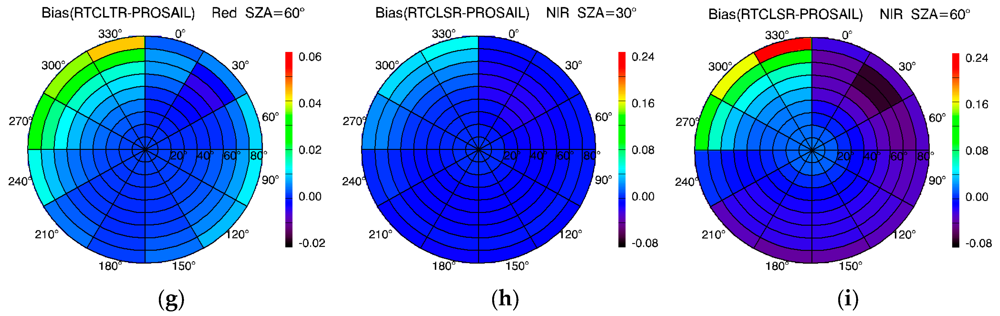
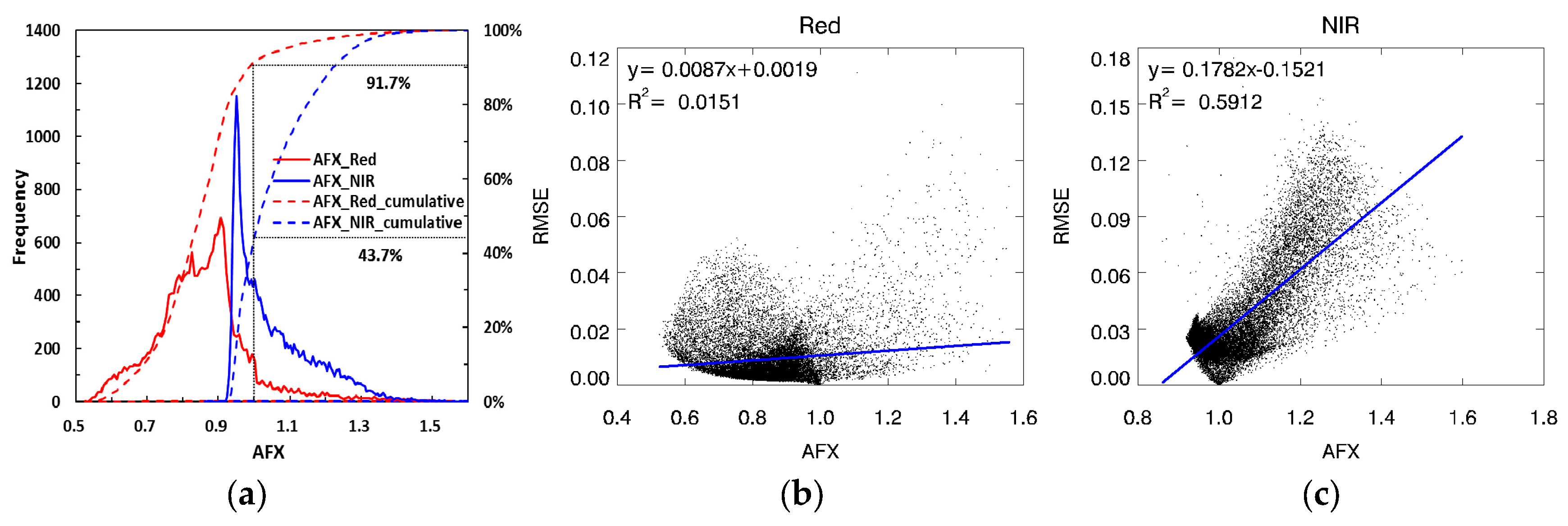
2 > 0.92), where 88.6% and 79.0% of fit-RMSEs are within tolerances of 0.02 and 0.05, respectively, in the two bands. This indicates great potential for linking these two models for potential applications, such as for developing inversion procedures to accurately retrieve vegetation properties from the satellite BRDF parameter product generated by the kernel-driven BRDF model. Limitations may arise from the few inconsistencies in BRFs between the two models in a large VZA beyond 70°, which somewhat depends on the variation of SZAs. In terms of reflectance anisotropy, geometric-optical scattering was dominant in the red band, whereas volumetric scattering was usually dominant in the NIR band. Model differences slightly increase for extreme case of volume scattering (large AFX values), especially in the NIR band. Additionally, attention should be paid to small LAI and Cab values and large ALA and P s o i l values in the red band, and large LAI and ALA values in the NIR band, which tend to result in more errors when linking the two models, especially for erectophile canopies. Great potential in linking the two models should arise based on the good agreement in albedo (R2 > 0.98), and 99.98% and 97.99% of the WSA deviations were less than 0.02 in the two bands. At an SZA of 30°, the BSA tends to perform best among all simulations. In addition, a similar result was found for the 21 sets of field BRDF observations, which presents more consistency between the two models than the result of the 20,000 PROSAIL simulations. This may contribute to the real measurements of BRDF and vegetation structure.
The overall good consistency between the two models suggests a great potential for linking these two models for parameter estimation, especially from the BRDF parameter product generated by the kernel-driven BRDF model, except for extreme cases that involve a few types of canopies. Therefore, future research should focus on the application of prior BRDF knowledge derived from the kernel-driven model, such as global BRDF parameters (e.g., MCD43A) and AFX BRDF archetypes, in conjunction with the PROSAIL inversion to devise an inversion relationship between vegetation structure and model BRDF parameters, based on the findings in this study.

Acknowledgments

This work is supported by the National Key Research and Development Program of China (No. 2016YFB0501404) and the National Science Foundation of China (No. 41571326). We thank the PROSAIL Team for providing the model code online for free. The comments and recommendations by the anonymous reviewers are also greatly appreciated.

Author Contributions

Ziti Jiao helped to conceive the research. Xiaoning Zhang analyzed the data and wrote the original manuscript. Ziti Jiao and Yadong Dong helped review the paper. All authors have approved the manuscript.

Conflicts of Interest

The authors declare no conflicts of interest.

Abbreviations

ACRMA two-layer Canopy Reflectance Model
AFXAnisotropy Flat Index
ALAAverage Leaf Angle
ASKAngular and Spectral Kernel-driven Model
BRDFBidirectional Reflectance Distribution Function
BRFBidirectional Reflectance Factor
BSABlack Sky Albedo
CARCloud Absorption Radiometer
CIClumping Index
CRCanopy Reflectance
DARTDiscrete Anisotropic Radiative Transfer
FIFEFirst International Satellite Land Surface Climatology Project Field Experiment
LAILeaf Area Index
MODISModerate-resolution Imaging Spectroradiometer
NADINew Advanced Discrete Model
NDHDNormalized Difference between Hotspot and Darkspot
NIR Near Infrared
POLDERPolarization and Directionality of the Earth’s Reflectances
PROSAILPROSPECT (an optical Properties Spectra) and SAIL (Scattering by Arbitrarily Inclined Leaves)
RAMIRadiation Transfer Model Intercomparison
RMSERoot Mean Square Error
RTCLSRRoss Thick-Chen-Li Sparse-Reciprocal
RTCLTRRoss Thick-Chen-Li Transit-Reciprocal
RTLSRRoss Thick-Li Sparse-Reciprocal
SZASolar Zenith Angle
VZAView Zenith Angle
WoDWeight of Determination
WSAWhite Sky Albedo

References

  1. Jacquemoud, S.; Verhoef, W.; Baret, F.; Bacour, C.; Zarco-Tejada, P.J.; Asner, G.P.; François, C.; Ustin, S.L. PROSPECT+SAIL Models: A Review of Use for Vegetation Characterization. Remote Sens. Environ. 2009, 113, S56–S66. [Google Scholar] [CrossRef]
  2. Feret, J.; François, C.; Asner, G.P.; Gitelson, A.A.; Martin, R.E.; Bidel, L.P.; Ustin, S.L.; Le Maire, G.; Jacquemoud, S. PROSPECT-4 and 5: Advances in the Leaf Optical Properties Model Separating Photosynthetic Pigments. Remote Sens. Environ. 2008, 112, 3030–3043. [Google Scholar] [CrossRef]
  3. Verhoef, W.; Jia, L.; Xiao, Q.; Su, Z. Unified Optical-Thermal Four-Stream Radiative Transfer Theory for Homogeneous Vegetation Canopies. IEEE Trans. Geosci. Remote Sens. 2007, 45, 1808–1822. [Google Scholar] [CrossRef]
  4. Widlowski, J.L.; Taberner, M.; Pinty, B.; Bruniquel-Pinel, V.; Disney, M.; Fernandes, R.; Gastellu-Etchegorry, J.P.; Gobron, N.; Kuusk, A.; Lavergne, T.; et al. Third Radiation Transfer Model Intercomparison (RAMI) Exercise: Documenting Progress in Canopy Reflectance Models. J. Geophys. Res.-Atmos. 2007, 112. [Google Scholar] [CrossRef]
  5. Pinty, B.; Widlowski, J.L.; Taberner, M.; Gobron, N.; Verstraete, M.M.; Disney, M.; Gascon, F.; Gastellu, J.P.; Jiang, L.; Kuusk, A.; et al. Radiation Transfer Model Intercomparison (RAMI) Exercise: Results from the Second Phase. J. Geophys. Res.-Atmos. 2004, 109, 523–538. [Google Scholar] [CrossRef]
  6. Pinty, B.; Gobron, N.; Widlowski, J.L.; Gerstl, S.; Verstraete, M.M.; Antunes, M.; Bacour, C.; Gascon, F.; Gastellu, J.P.; Goel, N.; et al. Radiation Transfer Model Intercomparison (RAMI) Exercise. J. Geophys. Res.-Atmos. 2001, 106, 11937–11956. [Google Scholar] [CrossRef]
  7. Ren, H.; Liu, R.; Yan, G.; Li, Z.; Qin, Q.; Liu, Q.; Nerry, F. Performance Evaluation of Four Directional Emissivity Analytical Models with Thermal SAIL Model and Airborne Images. Opt. Express 2015, 23, A346–A360. [Google Scholar] [CrossRef] [PubMed]
  8. You, D.; Wen, J.; Liu, Q.; Liu, Q.; Tang, Y. The Angular and Spectral Kernel-Driven Model: Assessment and Application. IEEE J. Sel. Top. Appl. Earth Obs. Remote Sens. 2014, 7, 1331–1345. [Google Scholar]
  9. Kuusk, A. A Two-Layer Canopy Reflectance Model. J. Quant. Spectrosc. Radiat. Transf. 2001, 71, 1–9. [Google Scholar] [CrossRef]
  10. Gobron, N.; Pinty, B.; Verstraete, M.M.; Govaerts, Y. A Semidiscrete Model for the Scattering of Light by Vegetation. J. Geophys. Res.-Atmos. 1997, 102, 9431–9446. [Google Scholar] [CrossRef]
  11. Leblanc, S.G.; Chen, J.M. A Windows Graphic User Interface (GUI) for the Five-Scale Model for Fast BRDF Simulations. Remote Sens. Rev. 2000, 19, 293–305. [Google Scholar] [CrossRef]
  12. Dawson, T.P.; Curran, P.J.; Plummer, S.E. LIBERTY—Modeling the Effects of Leaf Biochemical Concentration on Reflectance Spectra. Remote Sens. Environ. 1998, 65, 50–60. [Google Scholar] [CrossRef]
  13. Chen, J.M.; Leblanc, S.G. A Four-Scale Bidirectional Reflectance Model Based on Canopy Architecture. IEEE Trans. Geosci. Remote Sens. 1997, 35, 1316–1337. [Google Scholar] [CrossRef]
  14. Nicodemus, F.E.; Richmond, J.C.; Hsia, J.J.; Ginsberg, I.W.; Limperis, T. Geometrical Considerations and Nomenclature for Reflectance; Richmond, J., Ed.; National Bureau of Standards: Washington, DC, USA, 1977. [Google Scholar]
  15. Bacour, C.; Breon, F.M. Variability of Biome Reflectance Directional Signatures as Seen by POLDER. Remote Sens. Environ. 2005, 98, 80–95. [Google Scholar] [CrossRef]
  16. Jin, Y.F.; Schaaf, C.B.; Gao, F.; Li, X.W.; Strahler, A.H.; Lucht, W.; Liang, S.L. Consistency of MODIS Surface Bidirectional Reflectance Distribution Function and Albedo Retrievals: 1. Algorithm Performance. J. Geophys. Res.-Atmos. 2003, 108. [Google Scholar] [CrossRef]
  17. Lucht, W.; Schaaf, C.B.; Strahler, A.H. An Algorithm for the Retrieval of Albedo from Space Using Semiempirical BRDF Models. IEEE Trans. Geosci. Remote Sens. 2000, 38, 977–998. [Google Scholar] [CrossRef]
  18. Schaaf, C.B.; Gao, F.; Strahler, A.H.; Lucht, W.; Li, X.W.; Tsang, T.; Strugnell, N.C.; Zhang, X.Y.; Jin, Y.F.; Muller, J.P.; et al. First Operational BRDF, Albedo Nadir Reflectance Products from MODIS. Remote Sens. Environ. 2002, 83, 135–148. [Google Scholar] [CrossRef]
  19. Geiger, B.; Roujean, J.; Carrer, D.; Meurey, C. Product User Manual (PUM) Land Surface Albedo; LSA SAF Internal Documents; Eumetsat: Valencia, Spain, 2005; Volume 41, Available online: https://landsaf.ipma.pt/en/products/albedo/ (accessed on 20 January 2018).
  20. Martonchik, J.V.; Diner, D.J.; Pinty, B.; Verstraete, M.M.; Myneni, R.B.; Knyazikhin, Y.; Gordon, H.R. Determination of Land and Ocean Reflective, Radiative, and Biophysical Properties Using Multiangle Imaging. IEEE Trans. Geosci. Remote Sens. 1998, 36, 1266–1281. [Google Scholar] [CrossRef]
  21. Xiao, Z.; Liang, S.; Wang, J.; Xie, D.; Song, J.; Fensholt, R. A Framework for Consistent Estimation of Leaf Area Index, Fraction of Absorbed Photosynthetically Active Radiation, and Surface Albedo from MODIS Time-Series Data. IEEE Trans. Geosci. Remote Sens. 2015, 53, 3178–3197. [Google Scholar] [CrossRef]
  22. Zhou, H.; Wang, J.; Liang, S.; Xiao, Z. Extended Data-Based Mechanistic Method for Improving Leaf Area Index Time Series Estimation with Satellite Data. Remote Sens. 2017, 9, 533. [Google Scholar] [CrossRef]
  23. Yi, Y.; Yang, D.; Huang, J.; Chen, D. Evaluation of MODIS Surface Reflectance Products for Wheat Leaf Area Index (LAI) Retrieval. Isprs J. Photogramm. Remote Sens. 2008, 63, 661–677. [Google Scholar] [CrossRef]
  24. Wang, L.; Dong, T.; Zhang, G.; Niu, Z. LAI Retrieval Using PROSAIL Model and Optimal Angle Combination of Multi-Angular Data in Wheat. IEEE J. Sel. Top. Appl. Earth Obs. Remote Sens. 2013, 6, 1730–1736. [Google Scholar] [CrossRef]
  25. He, L.; Chen, J.M.; Pisek, J.; Schaaf, C.B.; Strahler, A.H. Global Clumping Index Map Derived from the MODIS BRDF Product. Remote Sens. Environ. 2012, 119, 118–130. [Google Scholar] [CrossRef]
  26. Chen, J.M.; Menges, C.H.; Leblanc, S.G. Global Mapping of Foliage Clumping Index Using Multi-Angular Satellite Data. Remote Sens. Environ. 2005, 97, 447–457. [Google Scholar] [CrossRef]
  27. Jiao, Z.; Dong, Y.; Schaaf, C.B.; Chen, J.M.; Román, M.; Wang, Z.; Zhang, H.; Ding, A.; Erb, A.; Hill, M.J.; et al. An Algorithm for the Retrieval of the Clumping Index (CI) from the MODIS BRDF Product Using an Adjusted Version of the Kernel-Driven BRDF Model. Remote Sens. Environ. 2018, in press. [Google Scholar]
  28. Wang, Z.; Schaaf, C.B.; Lewis, P.; Knyazikhin, Y.; Schull, M.A.; Strahler, A.H.; Yao, T.; Myneni, R.B.; Chopping, M.J.; Blair, B.J. Retrieval of Canopy Height Using Moderate-Resolution Imaging Spectroradiometer (MODIS) Data. Remote Sens. Environ. 2011, 115, 1595–1601. [Google Scholar] [CrossRef]
  29. Verhoef, W. Light-Scattering by Leaf Layers with Application to Canopy Reflectance Modeling—The SAIL Model. Remote Sens. Environ. 1984, 16, 125–141. [Google Scholar] [CrossRef]
  30. Wanner, W.; Li, X.; Strahler, A.H. On the Derivation of Kernels for Kernel-Driven Models of Bidirectional Reflectance. J. Geophys. Res.-Atmos. 1995, 100, 21077–21089. [Google Scholar] [CrossRef]
  31. Roujean, J.L.; Leroy, M.; Deschamps, P.Y. A Bidirectional Reflectance Model of the Earths Surface for the Correction of Remote-Sensing Data. J. Geophys. Res.-Atmos. 1992, 97, 20455–20468. [Google Scholar] [CrossRef]
  32. Lucht, W.; Roujean, J.L. Considerations in the Parametric Modeling of BRDF and Albedo from Multiangular Satellite Sensor Observations. Remote Sens. Rev. 2000, 18, 343–379. [Google Scholar] [CrossRef]
  33. Jiao, Z.; Schaaf, C.B.; Dong, Y.; Roman, M.; Hill, M.J.; Chen, J.M.; Wang, Z.; Zhang, H.; Saenz, E.; Poudyal, R.; et al. A Method for Improving Hotspot Directional Signatures in BRDF Models Used for MODIS. Remote Sens. Environ. 2016, 186, 135–151. [Google Scholar] [CrossRef]
  34. Li, X.W.; Strahler, A.H. Geometric-Optical Bidirectional Reflectance Modeling of the Discrete Crown Vegetation Canopy—Effect of Crown Shape and Mutual Shadowing. IEEE Trans. Geosci. Remote Sens. 1992, 30, 276–292. [Google Scholar] [CrossRef]
  35. Lucht, W.; Lewis, P. Theoretical Noise Sensitivity of BRDF and Albedo Retrieval from the EOS-MODIS and MISR Sensors with Respect to Angular Sampling. Int. J. Remote Sens. 2000, 21, 81–98. [Google Scholar] [CrossRef]
  36. Li, X.; Gao, F.; Chen, L.; Strahler, A.H. Derivation and Validation of a New Kernel for Kernel-Driven BRDF Models. Proc. SPIE 1999, 3868, 368–379. [Google Scholar]
  37. Dong, Y.; Jiao, Z.; Zhang, H.; Bai, D.; Zhang, X.; Li, Y.; He, D. A Visualization Tool for the Kernel-Driven Model with Improved Ability in Data Analysis and Kernel Assessment. Comput. Geosci. 2016, 95, 1–10. [Google Scholar] [CrossRef]
  38. Zhang, H.; Jiao, Z.; Dong, Y.; Du, P.; Li, Y.; Lian, Y.; Cui, T. Analysis of Extracting Prior BRDF from MODIS BRDF Data. Remote Sens. 2016, 8, 1004. [Google Scholar] [CrossRef]
  39. Zhang, H.; Jiao, Z.; Dong, Y.; Li, X. Evaluation of BRDF Archetypes for Representing Surface Reflectance Anisotropy Using MODIS BRDF Data. Remote Sens. 2015, 7, 7826–7845. [Google Scholar] [CrossRef]
  40. Jiao, Z.; Hill, M.J.; Schaaf, C.B.; Zhang, H.; Wang, Z.; Li, X. An Anisotropic Flat Index (AFX) to Derive BRDF Archetypes from MODIS. Remote Sens. Environ. 2014, 141, 168–187. [Google Scholar] [CrossRef]
  41. Roman, M.O.; Gatebe, C.K.; Schaaf, C.B.; Poudyal, R.; Wang, Z.; King, M.D. Variability in Surface BRDF at Different Spatial Scales (30 M–500 M) Over a Mixed Agricultural Landscape as Retrieved from Airborne and Satellite Spectral Measurements. Remote Sens. Environ. 2011, 115, 2184–2203. [Google Scholar] [CrossRef]
  42. Allen, W.A.; Gausman, H.W.; Richards, A.J.; Thomas, J.R. Interaction of Isotropic Light with a Compact Plant Leaf. J. Opt. Soc. Am. 1969, 59, 1376–1379. [Google Scholar] [CrossRef]
  43. Xiao, Y.; Zhao, W.; Zhou, D.; Gong, H. Sensitivity Analysis of Vegetation Reflectance to Biochemical and Biophysical Variables at Leaf, Canopy, and Regional Scales. IEEE Trans. Geosci. Remote Sens. 2014, 52, 4014–4024. [Google Scholar] [CrossRef]
  44. Bacour, C.; Jacquemoud, S.; Tourbier, Y.; Dechambre, M.; Frangi, J.P. Design and Analysis of Numerical Experiments to Compare Four Canopy Reflectance Models. Remote Sens. Environ. 2002, 79, 72–83. [Google Scholar] [CrossRef]
  45. Saltelli, A.; Tarantola, S.; Chan, K. A Quantitative Model-Independent Method for Global Sensitivity Analysis of Model Output. Technometrics 1999, 41, 39–56. [Google Scholar] [CrossRef]
  46. Schaepman-Strub, G.; Schaepman, M.E.; Painter, T.H.; Dangel, S.; Martonchik, J.V. Reflectance Quantities in Optical Remote Sensing-Definitions and Case Studies. Remote Sens. Environ. 2006, 103, 27–42. [Google Scholar] [CrossRef]
  47. Sandmeier, S.R.; Strahler, A.H. BRDF Laboratory Measurements. Remote Sens. Rev. 2000, 18, 481–502. [Google Scholar] [CrossRef]
  48. Qu, Y.; Liu, Q.; Liang, S.; Wang, L.; Liu, N.; Liu, S. Direct-Estimation Algorithm for Mapping Daily Land-Surface Broadband Albedo from MODIS Data. IEEE Trans. Geosci. Remote Sens. 2014, 52, 907–919. [Google Scholar] [CrossRef]
  49. Boréon, F.M.; Maignan, F. A BRDF–BPDF Database for the Analysis of Earth Target Reflectances. Earth Syst. Sci. Data 2017, 9, 31–45. [Google Scholar] [CrossRef]
  50. Privette, J.L.; Eck, T.F.; Deering, D.W. Estimating Spectral Albedo and Nadir Reflectance through Inversion of Simple BRDF Models with AVHRR/MODIS-like Data. J. Geophys. Res.-Atmos. 1997, 102, 29529–29542. [Google Scholar] [CrossRef]
  51. Ranson, K.J.; Biehl, L.L.; Bauer, M.E. Variation in Spectral Response of Soybeans with Respect to Illumination, View and Canopy Geometry. Int. J. Remote Sens. 1985, 6, 1827–1842. [Google Scholar] [CrossRef]
  52. Kimes, D.S.; Newcomb, W.W.; Nelson, R.F.; Schutt, J.B. Directional Reflectance Distributions of a Hardwood and Pine Forest Canopy. IEEE Trans. Geosci. Remote Sens. 1986, GE-24, 281–293. [Google Scholar] [CrossRef]
  53. Kimes, D.S. Dynamics of Directional Reflectance Factor Distributions for Vegetation Canopies. Appl. Opt. 1983, 22, 1364–1372. [Google Scholar] [CrossRef] [PubMed]
  54. Huang, X.; Jiao, Z.; Dong, Y.; Zhang, H.; Li, X. Analysis of BRDF and Albedo Retrieved by Kernel-Driven Models Using Field Measurements. IEEE J. Sel. Top. Appl. Earth Obs. Remote Sens. 2013, 6, 149–161. [Google Scholar] [CrossRef]
  55. Gao, F.; Li, X.; Strahler, A.; Schaaf, C. Evaluation of the Li Transit Kernel for BRDF Modeling. Remote Sens. Rev. 2000, 19, 205–224. [Google Scholar] [CrossRef]
  56. Hu, B.; Lucht, W.; Li, X.; Strahler, A.H. Validation of Kernel-Driven Semiempirical Models for the Surface Bidirectional Reflectance Distribution Function of Land Surfaces. Remote Sens. Environ. 1997, 62, 201–214. [Google Scholar] [CrossRef]
  57. Jacquemoud, S.; Baret, F. PROSPECT: A Model of Leaf Optical Properties Spectra. Remote Sens. Environ. 1990, 34, 75–91. [Google Scholar] [CrossRef]
  58. Enriquez, E.; Fuertes, V.; Cabrera, M.J.; Seores, J.; Munoz, D.; Fernandez, J.F. New Strategy to Mitigate Urban Heat Island Effect: Energy Saving by Combining High Albedo and Low Thermal Diffusivity in Glass Ceramic Materials. Sol. Energy 2017, 149, 114–124. [Google Scholar] [CrossRef]
  59. Dickinson, R.E. Land Surface Processes and Climate Surface Albedos and Energy-Balance. Adv. Geophys. 1983, 25, 305–353. [Google Scholar]
  60. The Global Observing System for Climate: Implementation Needs; GCOS: Geneva, Switzerland, 2016; p. 325.
  61. Jin, Y.F.; Schaaf, C.B.; Woodcock, C.E.; Gao, F.; Li, X.W.; Strahler, A.H.; Lucht, W.; Liang, S.L. Consistency of MODIS Surface Bidirectional Reflectance Distribution Function and Albedo Retrievals: 2. Validation. J. Geophys. Res.-Atmos. 2003, 108. [Google Scholar] [CrossRef]
  62. Shuai, Y.; Schaaf, C.B.; Strahler, A.H.; Liu, J.; Jiao, Z. Quality Assessment of BRDF/albedo Retrievals in MODIS Operational System. Geophys. Res. Lett. 2008, 35, 544–548. [Google Scholar] [CrossRef]
  63. Liu, J.; Schaaf, C.; Strahler, A.; Jiao, Z.; Shuai, Y.; Zhang, Q.; Roman, M.; Augustine, J.A.; Dutton, E.G. Validation of Moderate Resolution Imaging Spectroradiometer (MODIS) Albedo Retrieval Algorithm: Dependence of Albedo on Solar Zenith Angle. J. Geophys. Res.-Atmos. 2009, 114. [Google Scholar] [CrossRef]
  64. Fang, H.; Wei, S.; Liang, S. Validation of MODIS and CYCLOPES LAI Products Using Global Field Measurement Data. Remote Sens. Environ. 2012, 119, 43–54. [Google Scholar] [CrossRef]
Figure 1. Flowchart of model comparison between the kernel-driven model and PROSAIL model.
Remotesensing 10 00437 g001
Figure 2. BRDF and albedo comparison of RTCLSR/RTCLTR inversions and PROSAIL simulations for a typical canopy. (ac) the reflectance obtained by the PROSAIL simulations and RTCLSR and RTCLTR inversions for the entire viewing hemisphere in the red band; (d,e) the deviations in the red band; (f) BRDF of the RTCLSR/RTCLTR models along the principal plane in the red band, where a positive value of VZA on the horizontal axis indicates an observation on the same side as the solar or backward direction; (gi) the same as (df) but for the NIR band; and (j) albedo comparison, where the BSA is related to the SZA from 0 to 89°. Dotted lines refer to the same result as solid lines but for the NIR band, and solid and hollow points refer to the corresponding WSA in the red and NIR bands, respectively.
Remotesensing 10 00437 g002
Figure 3. Comparison of the directional reflectances between the PROSAIL simulation and RTCLSR inversion in the red and NIR bands for diverse canopies, where the two gray dashed lines show the 0.02 and 0.05 tolerances: (a,b) comparison of the directional reflectances of five equal density levels from 1 (maximum) to 5 (minimum) and (c) histogram of fit-RMSE. (dg) refer to the distribution of average biases of BRFs between the two models for the red band, where SZAs of 30° and 60° are involved. (h,i) refer to the similar results as (d) and (f) but for the NIR band.
Remotesensing 10 00437 g003aRemotesensing 10 00437 g003b
Figure 4. Relationships between fit-RMSE and AFX in the red and NIR bands: (a) histogram of AFX; (b) relationship for the red band; and (c) relationship for the NIR band.
Remotesensing 10 00437 g004
Figure 5. Sensitivity of fit-RMSE to vegetation components: (af) relationships between vegetation parameters and fit-RMSE and (gl) the normalized histograms of vegetation parameters inside (blue line, 88.6% [red band] and 79.0% [NIR band] in total) and outside (red line) of the RMSE tolerance, as in Figure 3c, where the ordinate values are the percentages of each total proportion.
Remotesensing 10 00437 g005
Figure 6. Comparison of simulated and inversion-based albedos for diverse canopies, where the two gray dashed lines show the 0.02 and 0.05 tolerances, respectively: (a) WSA comparison in the red band; (b) BSA in the infrared band; (c) WSA and BSA statistics; and (df) results corresponding to those in (ac) for the NIR band.
Remotesensing 10 00437 g006aRemotesensing 10 00437 g006b
Figure 7. Comparison of the directional reflectances between the PROSAIL simulation and RTLSR inversion in the red and NIR bands for 21 sets of observations, where the two gray dashed lines show the 0.02 and 0.05 tolerances: (a,b) comparison of the directional reflectances between the PROSAIL simulation and observations at five equal density levels from 1 (maximum) to 5 (minimum). (c,d) Comparison for RTLSR retrievals and observations. (eg) Relationships between bias and three parameters, which are AFX, LAI and ALA, respectively.
Remotesensing 10 00437 g007
Figure 8. Comparison of simulated and inversion-based albedos for observations, where the two gray dashed lines show the 0.02 and 0.05 tolerances, respectively: (a) WSA comparison in the red and NIR bands; (b) BSA comparison in the two bands.
Remotesensing 10 00437 g008
Table 1. The input parameters of the PROSAIL model.
ParameterUnitsCommon Value (range)
Leaf Scale
leaf structure parameter (Ns)--1.5 (1–3)
chlorophyll a and b contents (Cab)μg/cm250 (0–100)
carotenoid content (Car)μg/cm210 (5–30)
brown pigment content (Cbrown)--0
equivalent water thickness (Cw)cm0.015 (0.004–0.04)
leaf mass per unit leaf area (Cm)g/cm20.009 (0.0019–0.0165)
Canopy Scale
LAIm2/m23.5 (0–6)
average leaf angle (ALA)degrees (°)50 (0–90)
hot spot (Hspot)mm0.2 (0–1)
soil coefficient ( P s o i l )--0.1 (0–1)
diffuse/direct radiation (SKYL)%0 (0–100)
Observation geometry
SZAdegrees (°)30 (0–90)
VZAdegrees (°)0 (0–90)
relative azimuth angle ( φ )degrees (°)0 (0–180)
Table 2. The description of the 21 sets of BRDF field measurements.
NumLand CoverLAI (m2/m2)Coverage (%)Chlorosis (%)Cloud (%)SKYL (%)
1Corn 10.65250–5 400 6
2Hardwood 24.2079 00 6
3Lawn grass 19.90970–5 400 6
4Orchard grass 31.105030–40 400 6
5Soybean 24.60900–5 400 6
6Mixed grass1.50 1015
7Sand shinnery oak1.7560.2 5–10(SZA, λ )
8Grassland 31.39 ± 0.36 68.2 5010
9Grassland1.55 ± 0.53 4.7 5010
10Grassland 31.19 ± 0.53 36.7 5010
11Dense grass-like vegetation 30.94 ± 0.30 65.9 50–510
12Sparse grass 30.24 ± 0.05 42.9 5010
13Dense grass-like vegetation 30.60 ± 0.34 59.1 50–510
14Grassland 31.91 ± 0.49 43.9 50–510
15Sparse grass-like vegetation 30.12 ± 0.04 50.3 5010
16Grassland3.59 58
17Grassland4.06 1015
18Cotton 24.00 010
19Soybean 23.00 ± 0.5072 ± 4 10–2020
20Soybean 23.90 ± 0.6083 ± 3 1–2015
21Soybean 22.90 ± 0.4099 ± 1 010
1 The monocotyledons with Ns ranging from 1.0 to 1.5. 2 The dicotyledons with Ns ranging from 1.5 to 2.5. 3 The senescent leaves with Ns larger than 2.5. 4 The percent of visual chlorosis. 5 The percent of dry weight of standing dead leaves among the total standing dry weight for both green and dead leaves. 6 The fraction of diffuse sky radiance had been corrected for these data.
Table 3. The AFX and fit-RMSE statistics between the RTCLSR/RTCLTR and PROSAIL models for diverse canopies.
StatisticsAFXRedAFXNIRRMSERed(LSR)RMSENIR(LSR)RMSERed(LTR)RMSENIR(LTR)
Minimum0.530.860.00000.00000.00000.0000
Maximum1.561.600.11110.17450.11200.1745
Average0.851.050.00920.03550.01030.0355
Table 4. The albedo deviation percentages between RTCLSR inversion and PROSAIL simulations in different accuracy ranges (%).
BandErrorWSABSAtotalBSA0 1BSA15BSA30BSA45BSA60
Red[0, 0.02]98.7239.353.674.2510.7882.5395.52
[−0.02, 0)1.2659.3093.2594.5789.2117.332.13
(0.02, 0.05]0.010.600.510.290.000.002.21
[−0.05, −0.02)0.000.722.440.890.010.130.14
>0.050.010.030.130.000.000.000.00
<-0.050.000.000.000.000.000.010.00
NIR[0, 0.02]79.3336.9114.9118.9919.6962.0868.90
[−0.02, 0)18.6649.6064.3263.9979.6024.2315.82
(0.02, 0.05]0.814.779.3313.140.220.171.00
[−0.05, −0.02)0.094.990.000.000.4211.8412.71
>0.051.113.1911.443.880.070.030.53
<−0.050.000.540.000.000.001.651.04
1 BSA0 refers to the BSA when the SZA is zero (nadir), and BSA15, BSA30, BSA45 and BSA60 refer to the BSAs for SZAs of 15, 30, 45, and 60°, respectively.
Table 5. The statistics of the average error between the PROSAIL simulations/RTLSR inversions and observations for the four typical parameters in Figure 5, where the bias refers to the mean of their absolute values.
ErrorLAI ≤ 1(>1)ALA ≤ 40(>40)Cab ≤ 20(>20)Psoil ≤ 0.2(>0.2)
Bias_PROSAIL_Red0.0185(0.0151) 10.0125(0.0167) 10.0183(0.0135) 10.0168(0.0149)
RMSE_PROSAIL_Red0.0364(0.0258) 10.0190(0.0306) 10.0299(0.0277) 10.0249(0.0322) 1
RMSE_RTLSR_Red0.0156(0.0096) 10.0110(0.0110) 10.0120(0.0085) 10.0103(0.0118) 1
Bias_PROSAIL_NIR0.0463(0.0367)0.0141(0.0448) 1
RMSE_PROSAIL_NIR0.0743(0.0820) 10.0694(0.0827) 1
RMSE_RTLSR_NIR0.0346(0.0455) 10.0570(0.0395)
1 Error distribution is consistent with the results shown in Figure 5.

