Geometric Insight into the Control Allocation Problem for Open-Frame ROVs and Visualisation of Solution

 ,
,  ,
,
Abstract
:1. Introduction
2. Control Allocation Problem
2.1. Problem Definition
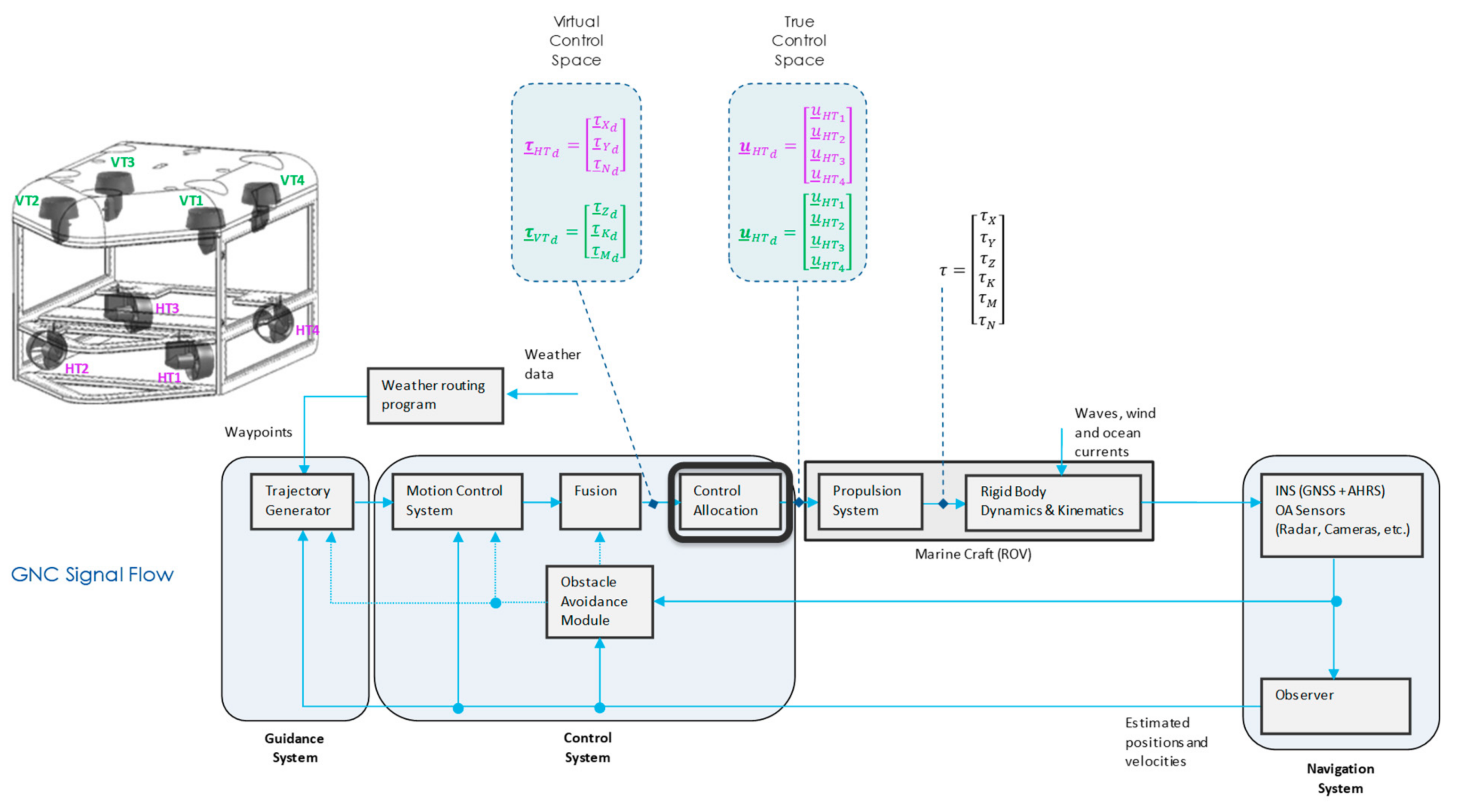
- Guidance: subsystem that continuously computes the reference (desired) position, velocity and acceleration of an ROV to be used by the motion control system.
- Navigation: subsystem to determine position/attitude, course, travelled distance and (optionally) velocity and acceleration of an ROV.
- Control: subsystem to determine necessary control forces and moments to be provided by the ROV to satisfy certain control objective (in conjunction with the guidance system).
- STEP 1 (Regulation Task): Design a control law, which specifies desired virtual control input (normalised vector of forces and moments ) in the virtual control space;
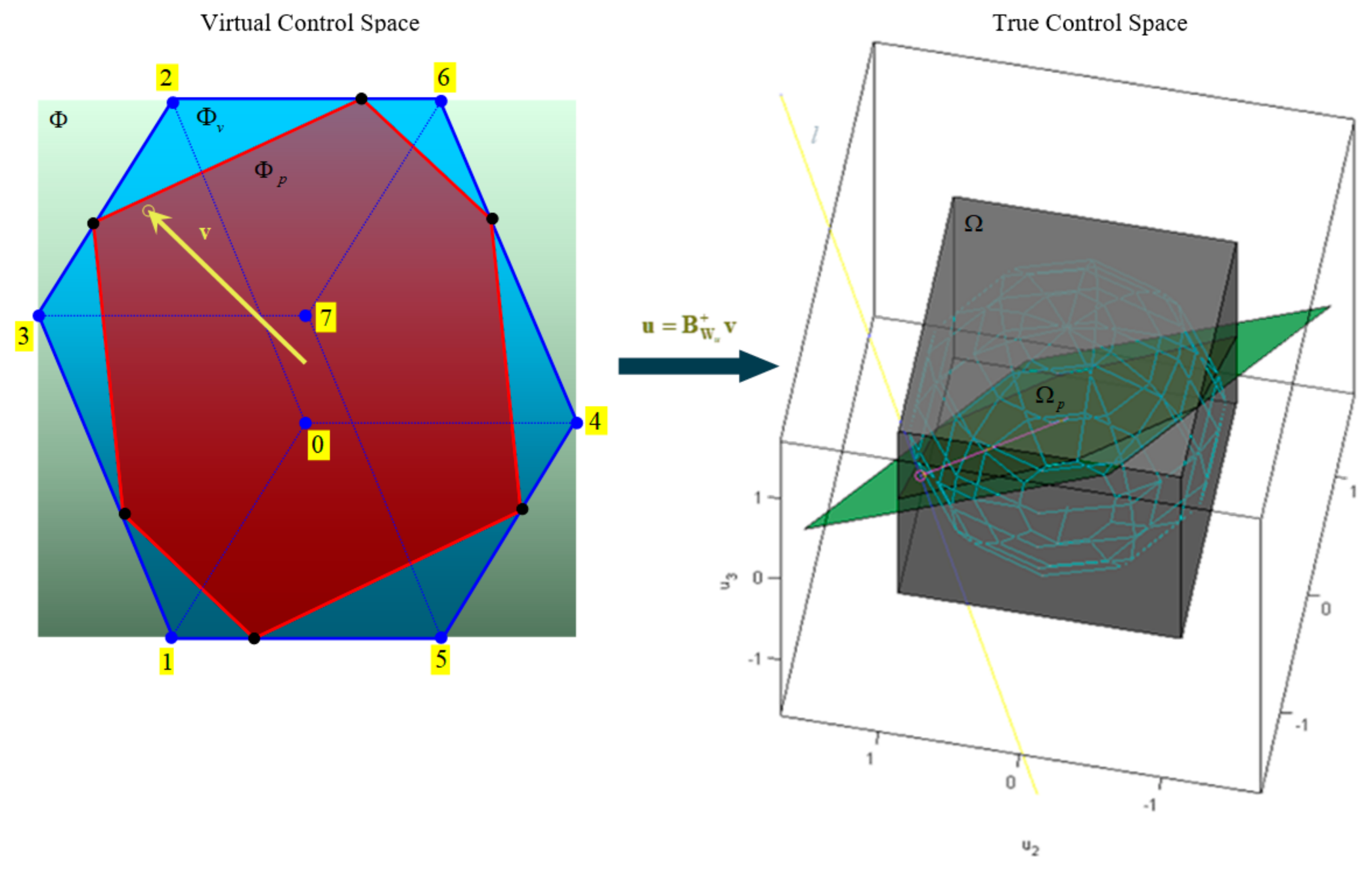
- STEP 2 (Actuator Selection Task): Design control allocator, which finds the “best” feasible true control input (normalised command vector to be applied to individual actuators) in the true control space.
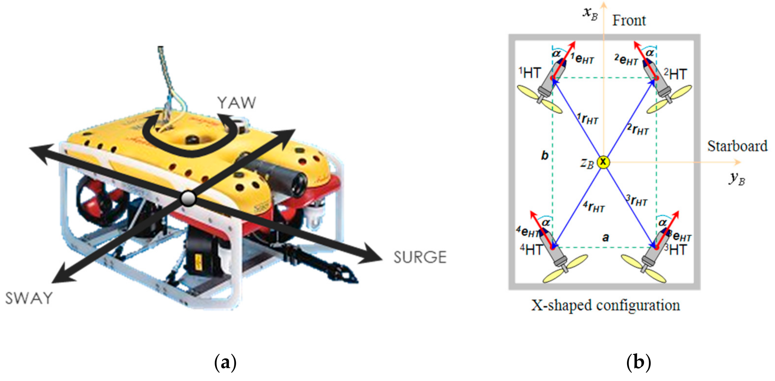
- —longitudinal axes (directed to front side),
- —transversal axes (directed to starboard),
- —normal axes (directed from top to bottom).
- is empty (i.e., no solution exists),
- has exactly one element (i.e., there is one unique solution),
- has more than one element (i.e., there are many solutions).
- If the intersection is a segment, there is an infinite number of solutions (each point that belongs to the segment is a solution),
- If the intersection is a point, there is only one solution,
- If the intersection is an empty set, no solution exists.
2.2. Nomenclature
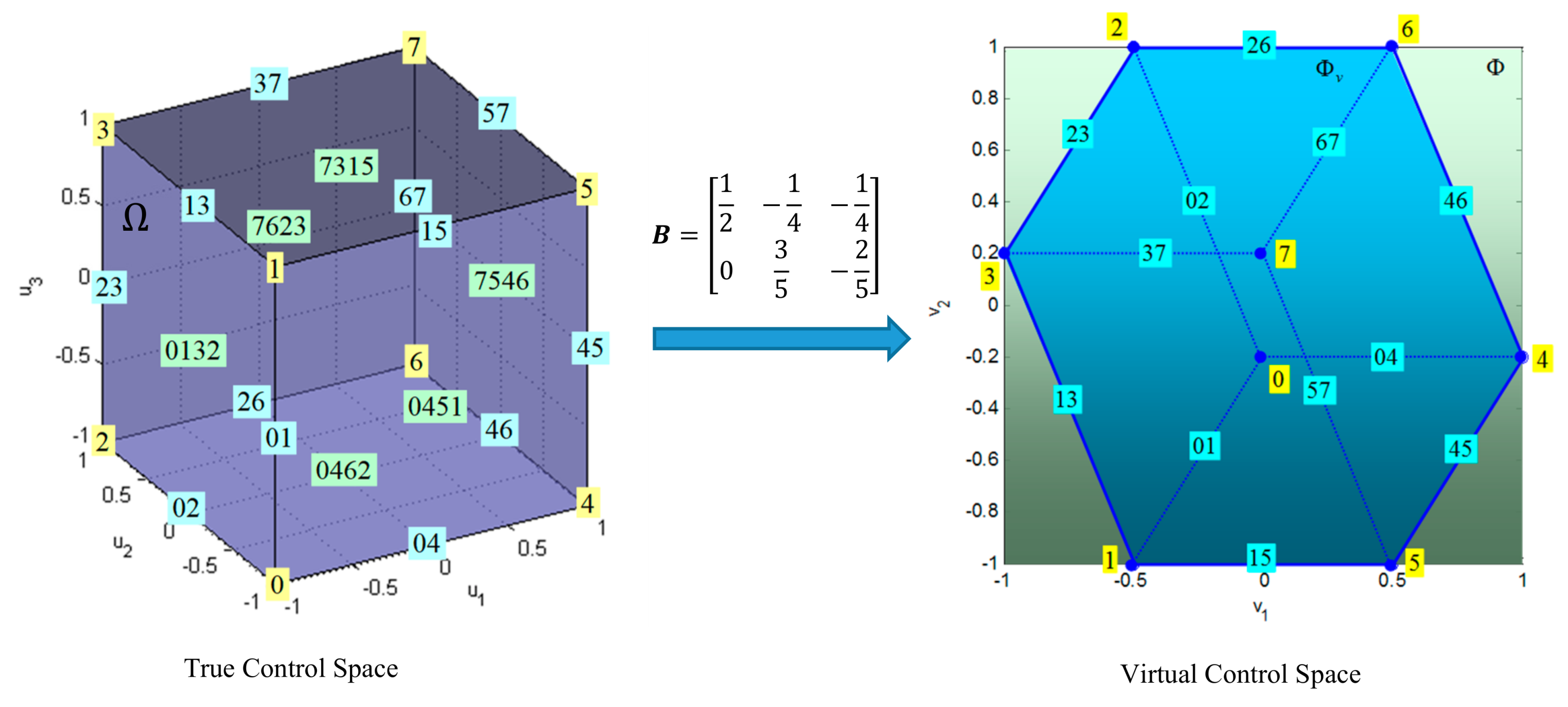
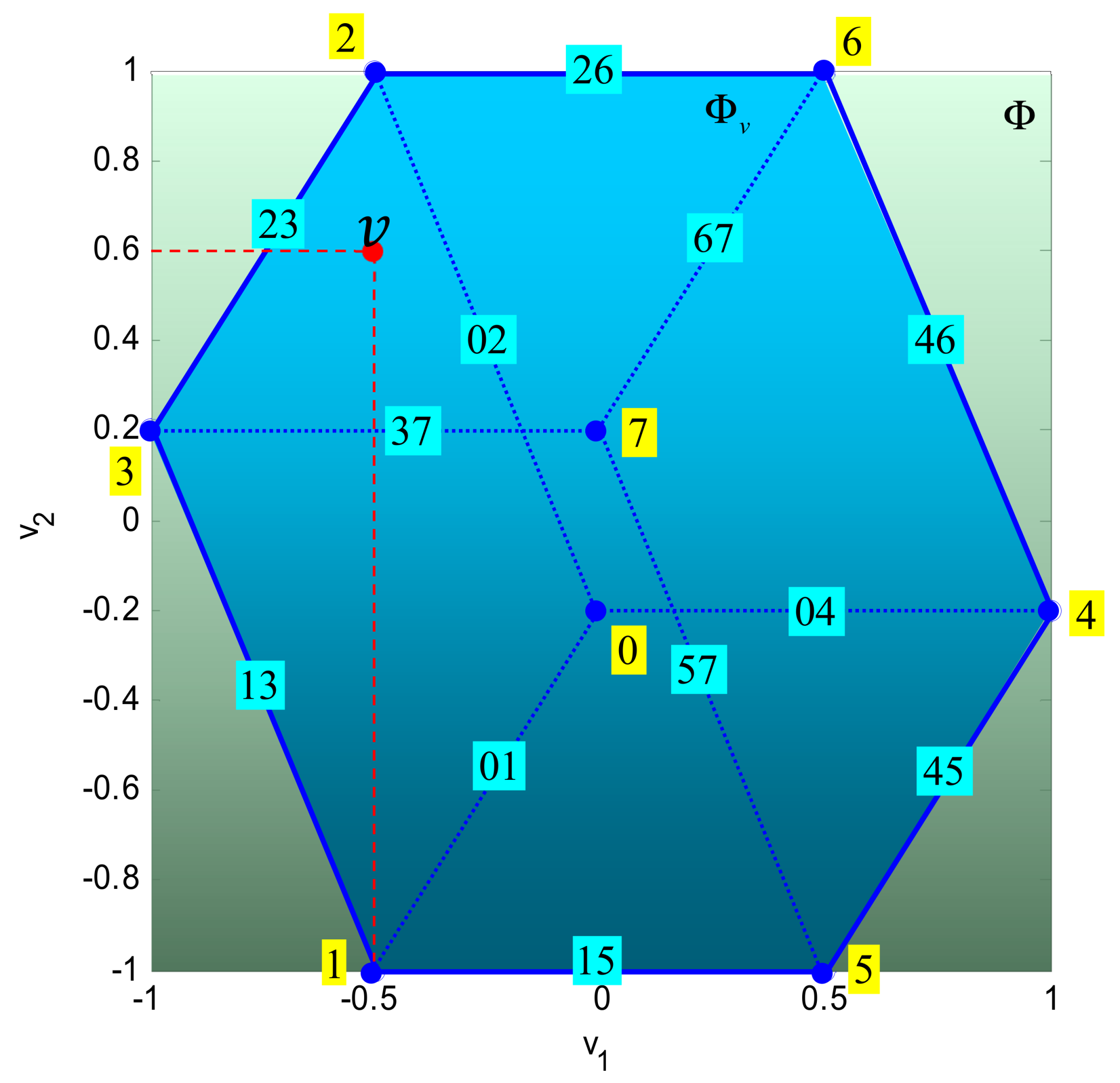
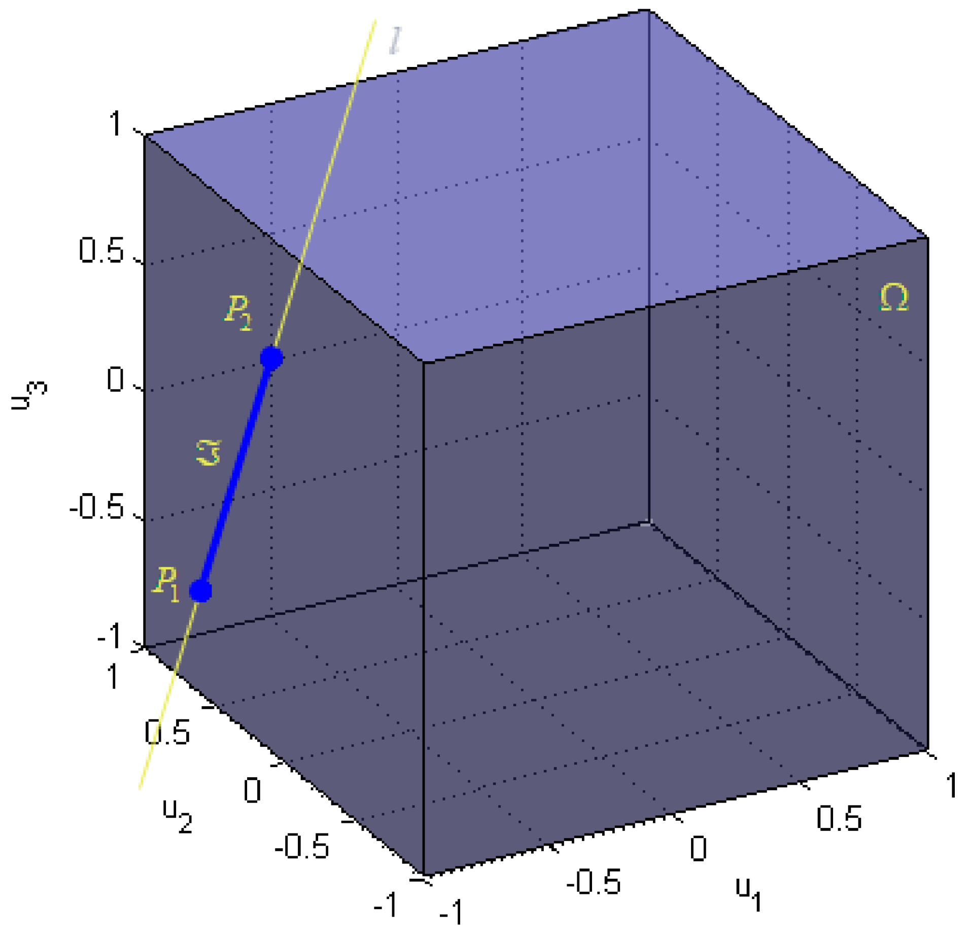
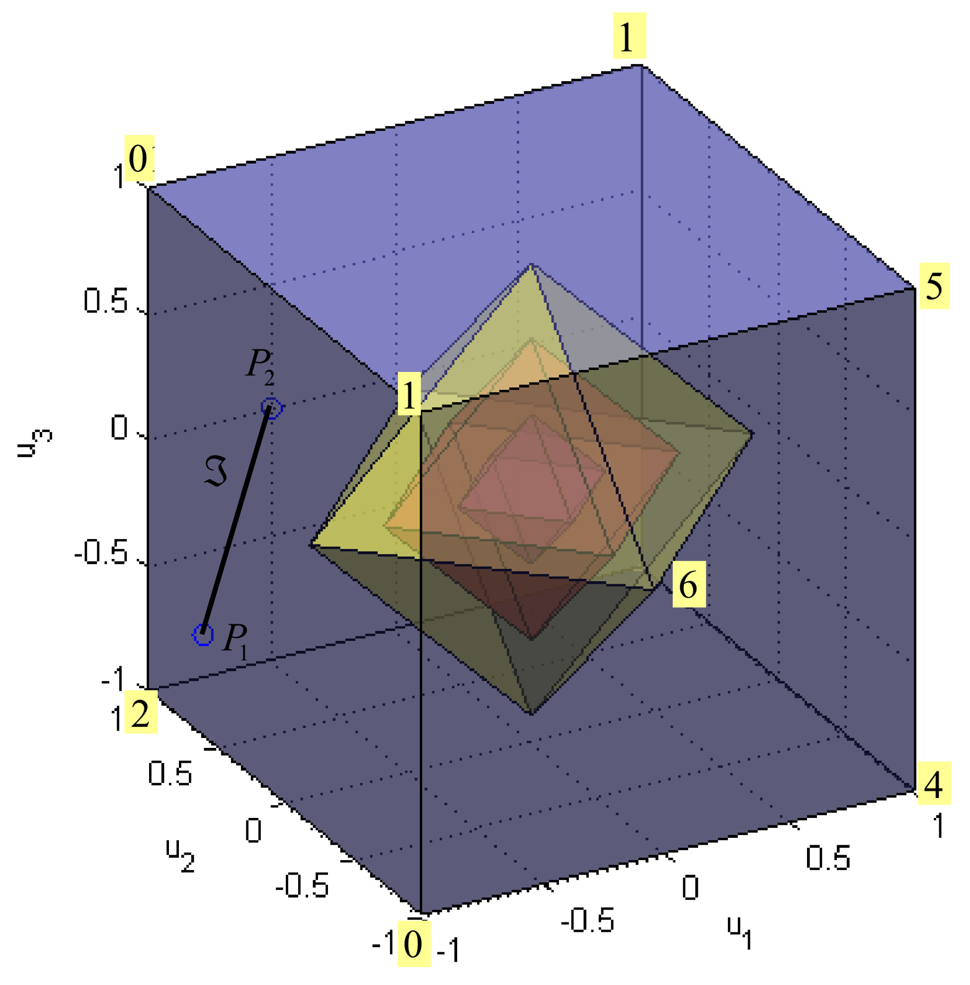
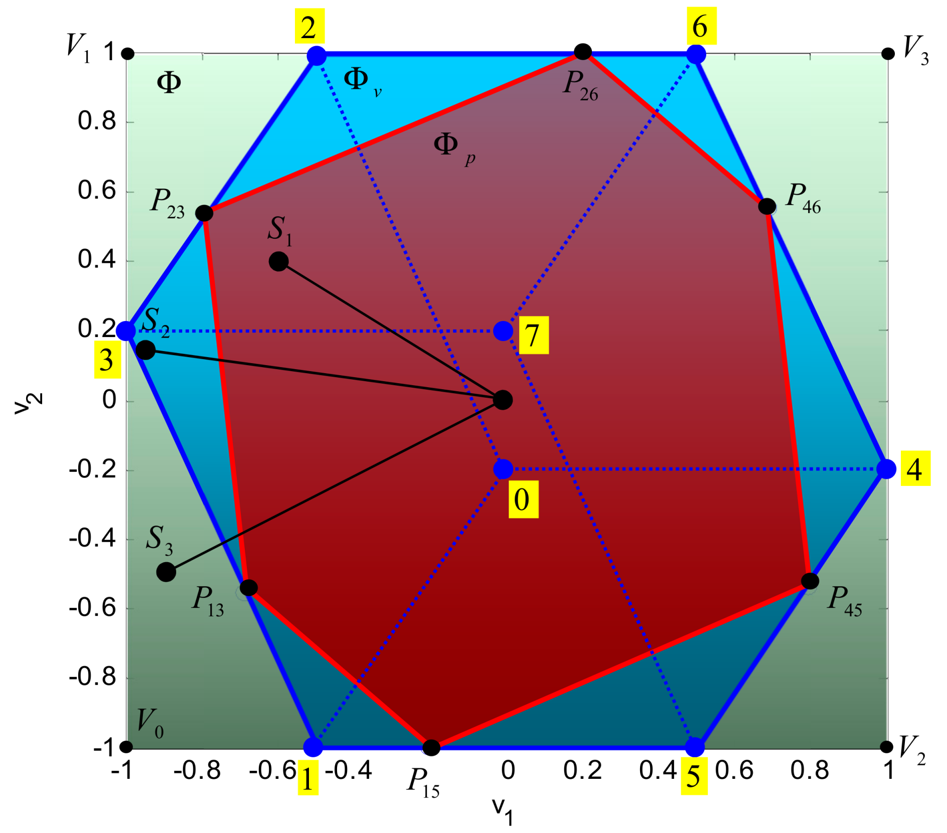
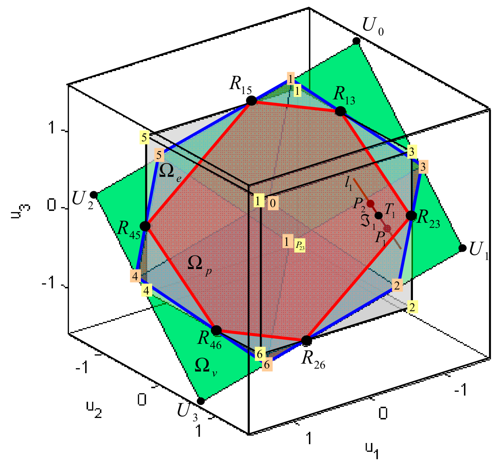
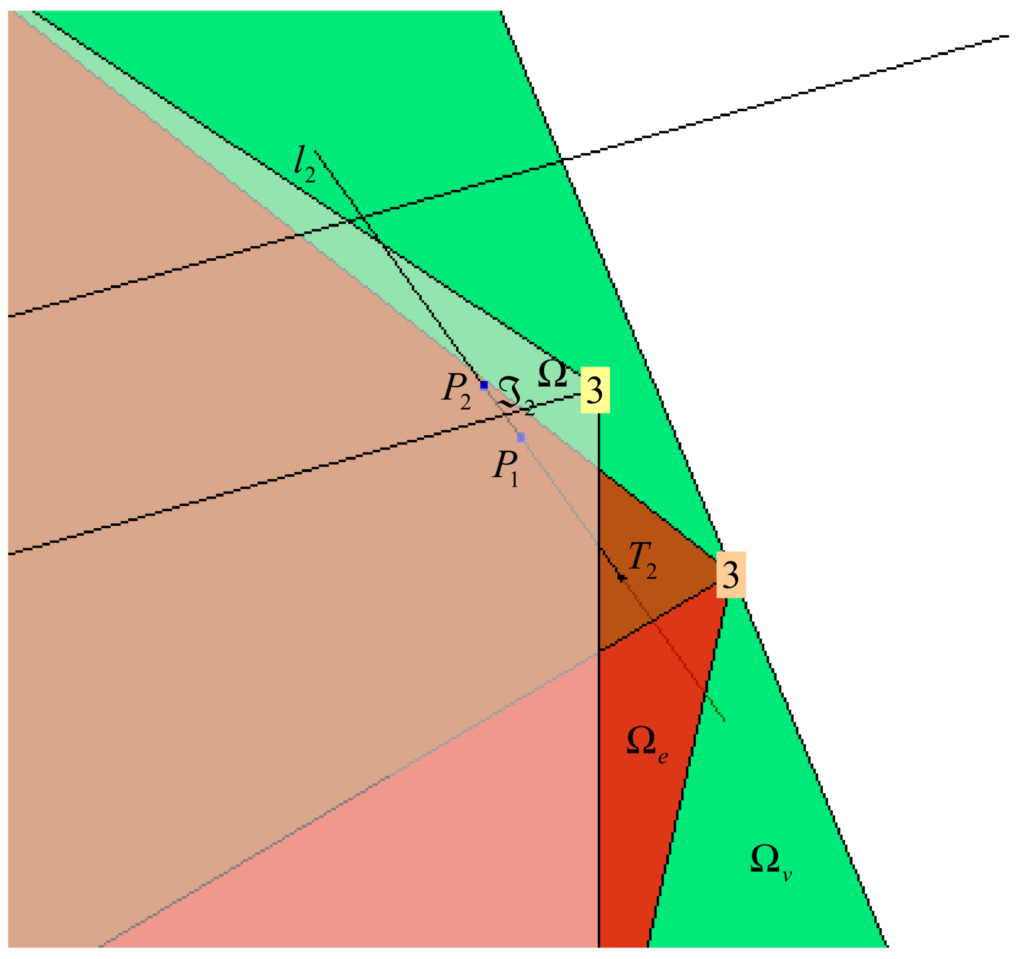
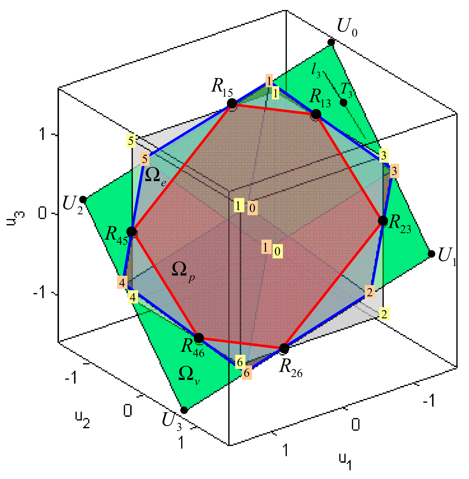
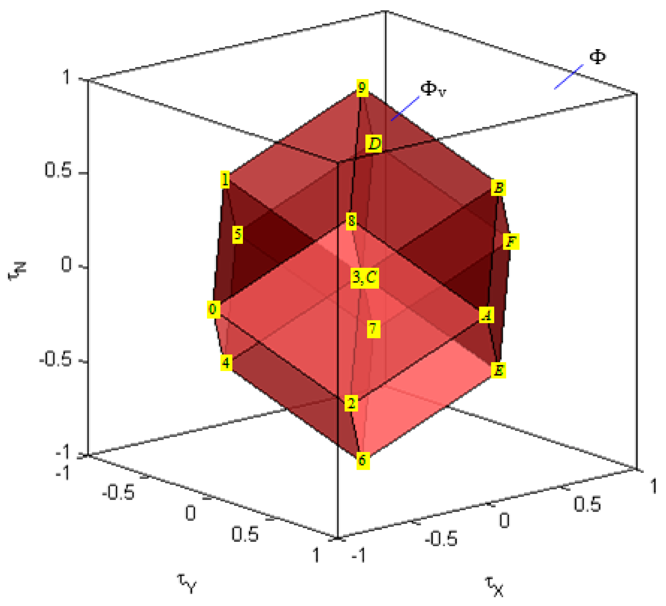
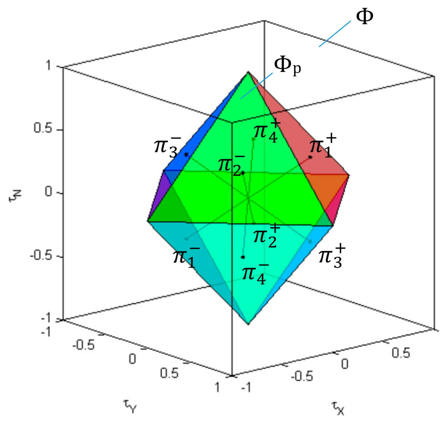
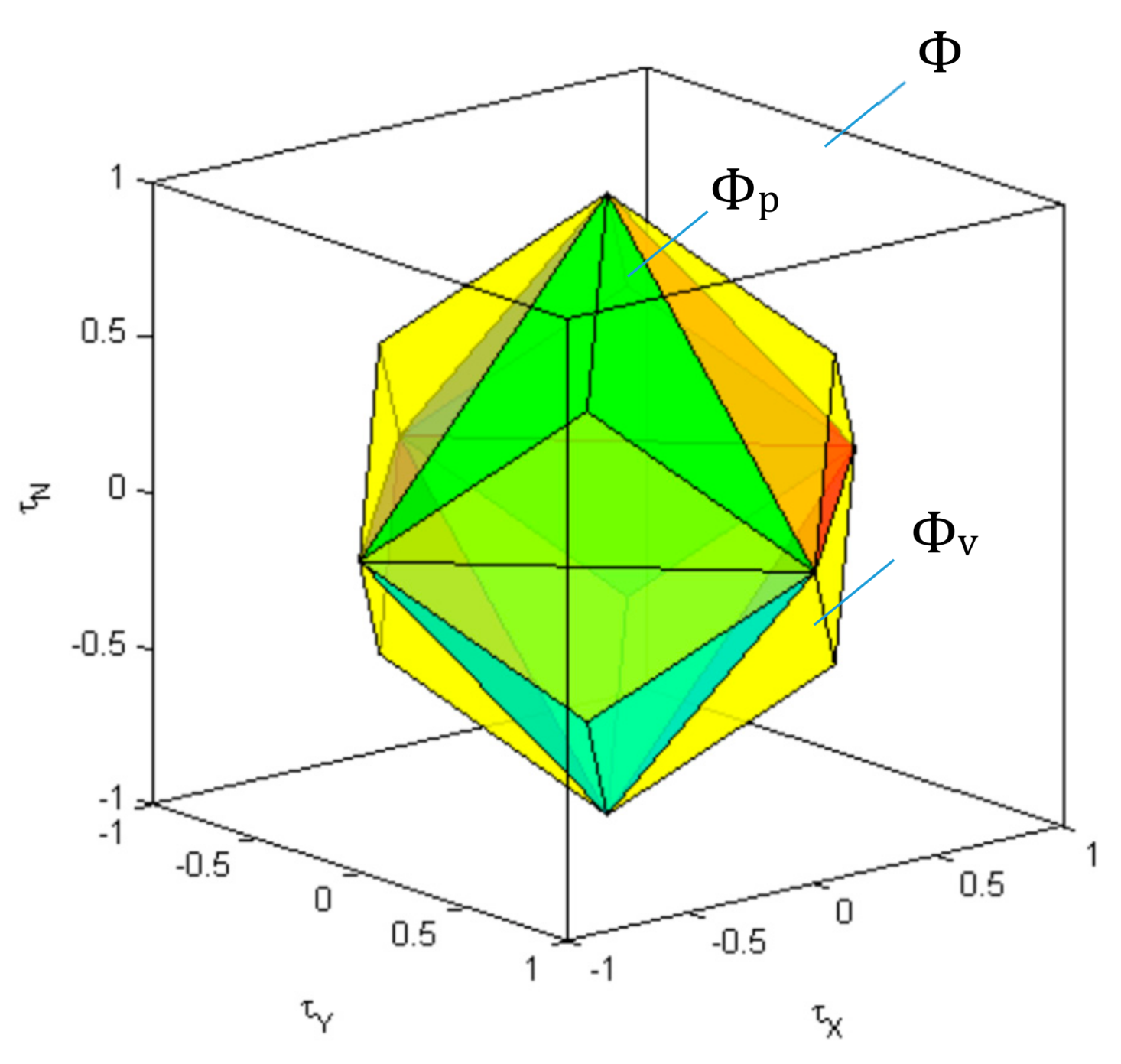
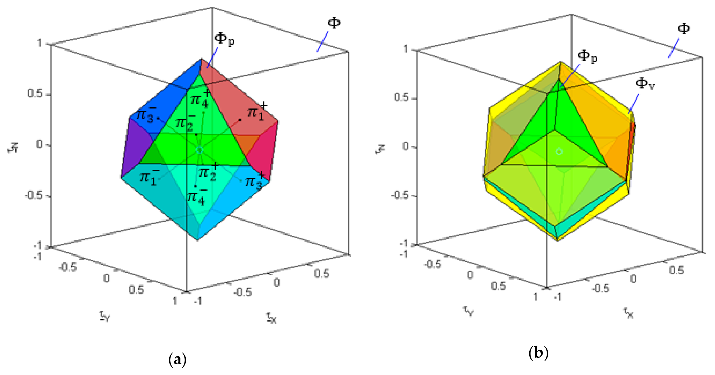
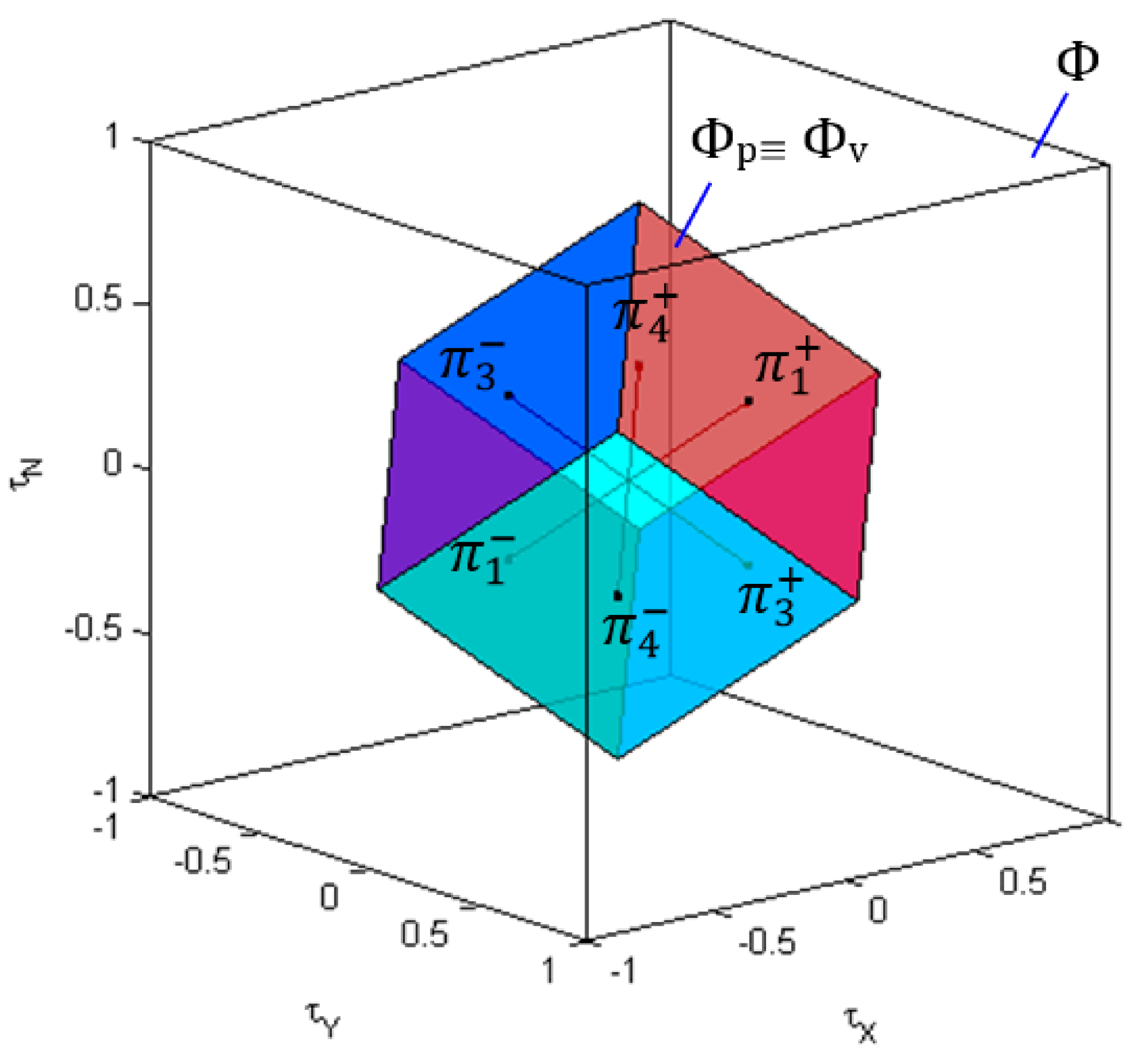
2.3. Geometric Insight into Problem
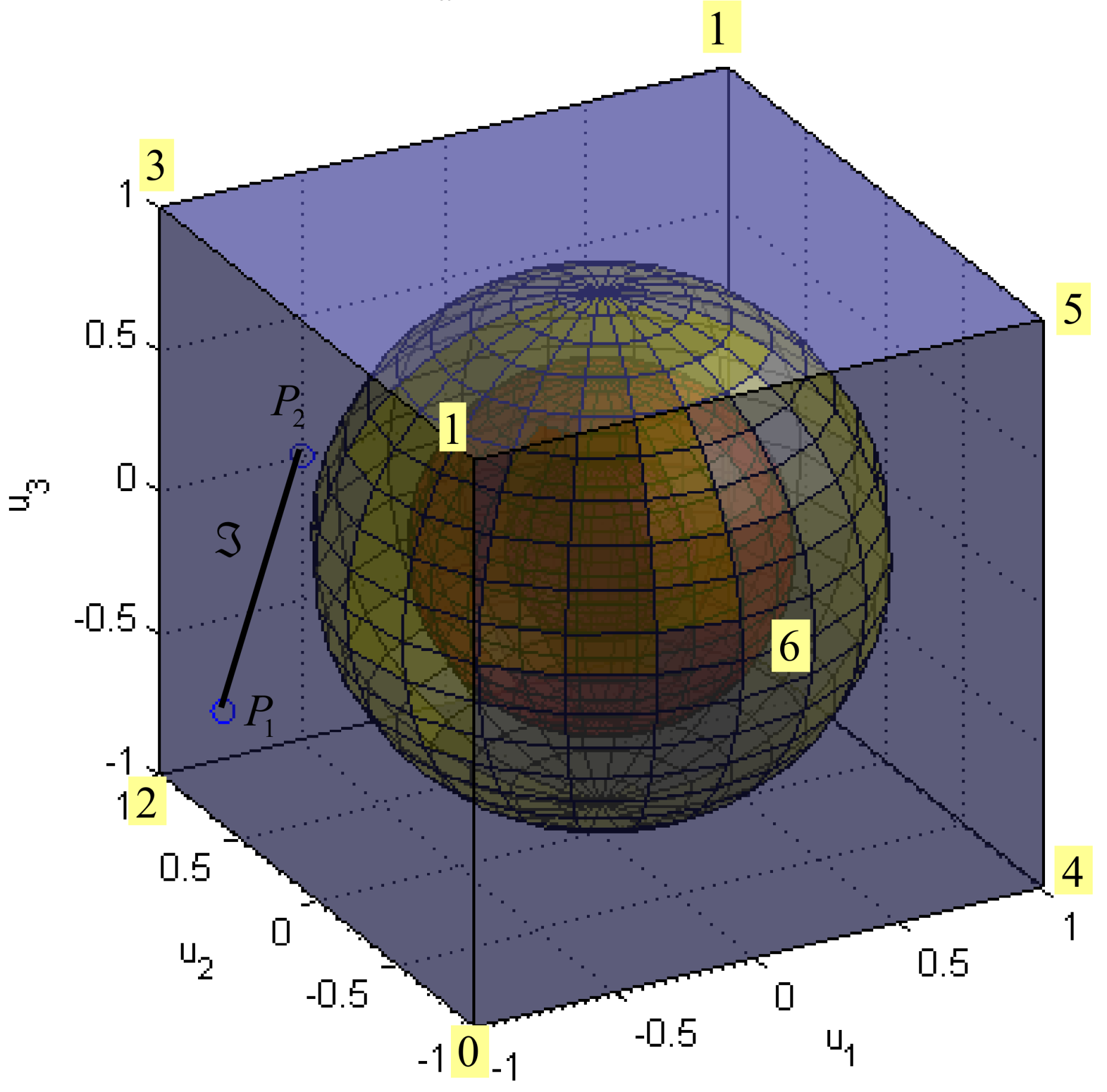
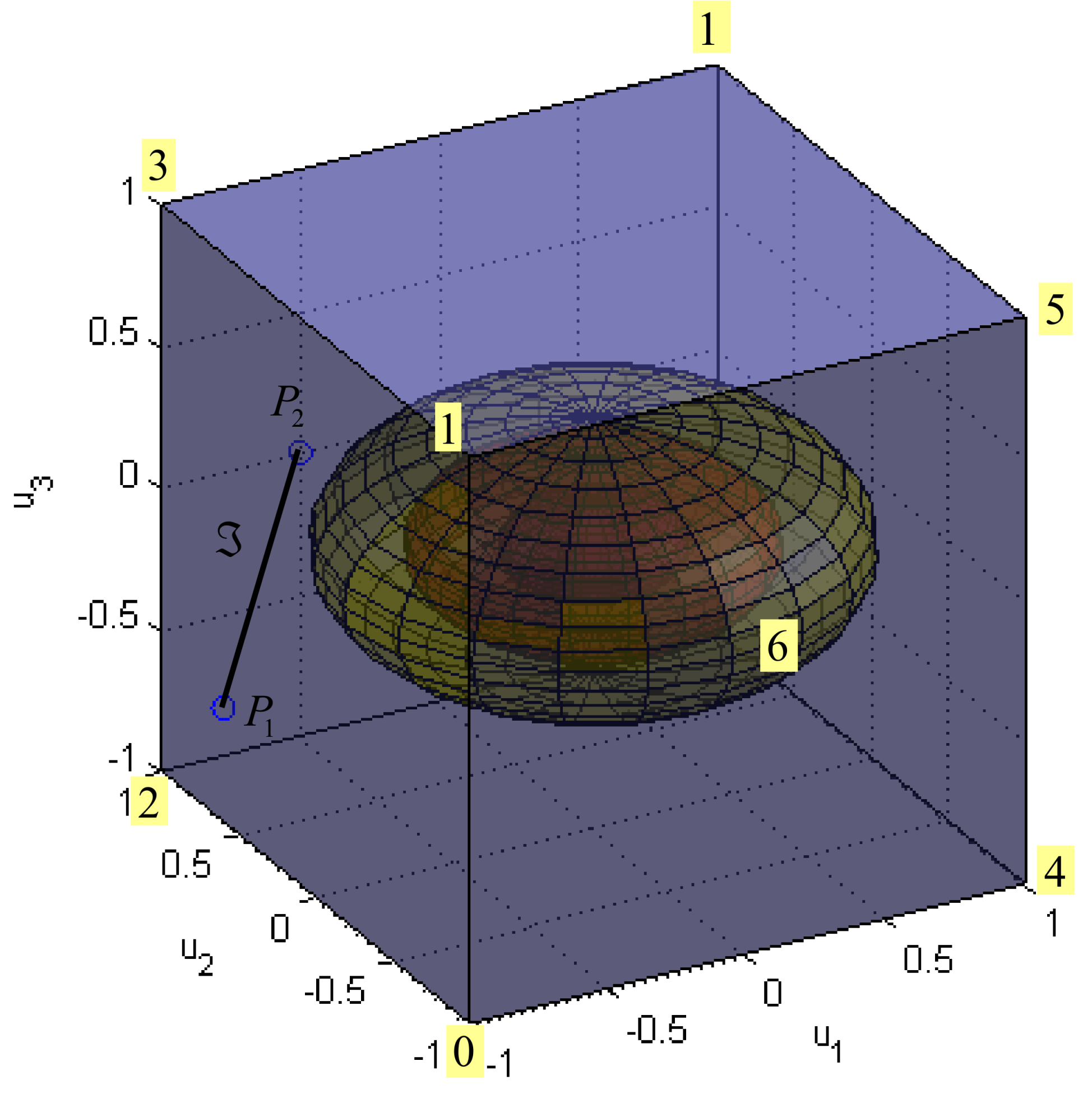
2.4. Choice of Norm
- In the case when is the unity matrix, the norm distributes the virtual control demand among the control inputs in a uniform way, while the solution utilises as few control inputs as possible to satisfy the virtual control demand.
- The solution varies continuously with the parameters (elements) of , while the solution does not. Change in a parameter (element) of will produce the change in the slope of . The solution will vary continuously with , while it can be shown that the solution will have discontinuity for some value of and the solution in the breakpoint is not unique.
- If is a non-singular, the problem has a unique solution for . For , this is not always the case, as discussed above. The reason lies in the fact that the sphere is a strictly convex set, while this is not the case for .
2.5. Choice of the Weighting Matrix
3. Control Allocation Solution: Hybrid Method
3.1. Description
3.2. Weighted Pseudoinverse
3.2.1. Introduction
- Find such that ,
- Find .
- 1.
- ,
- 2.
- ,
- 3.
- .
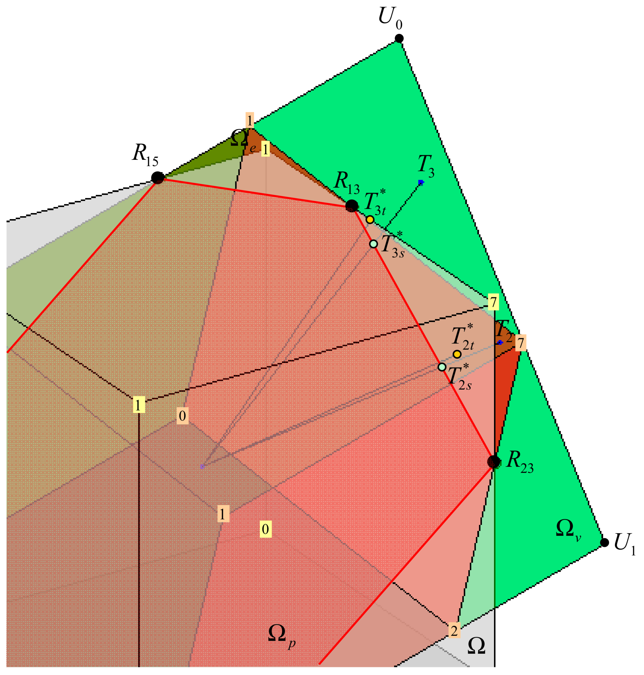
3.2.2. Approximation of Unfeasible Solution
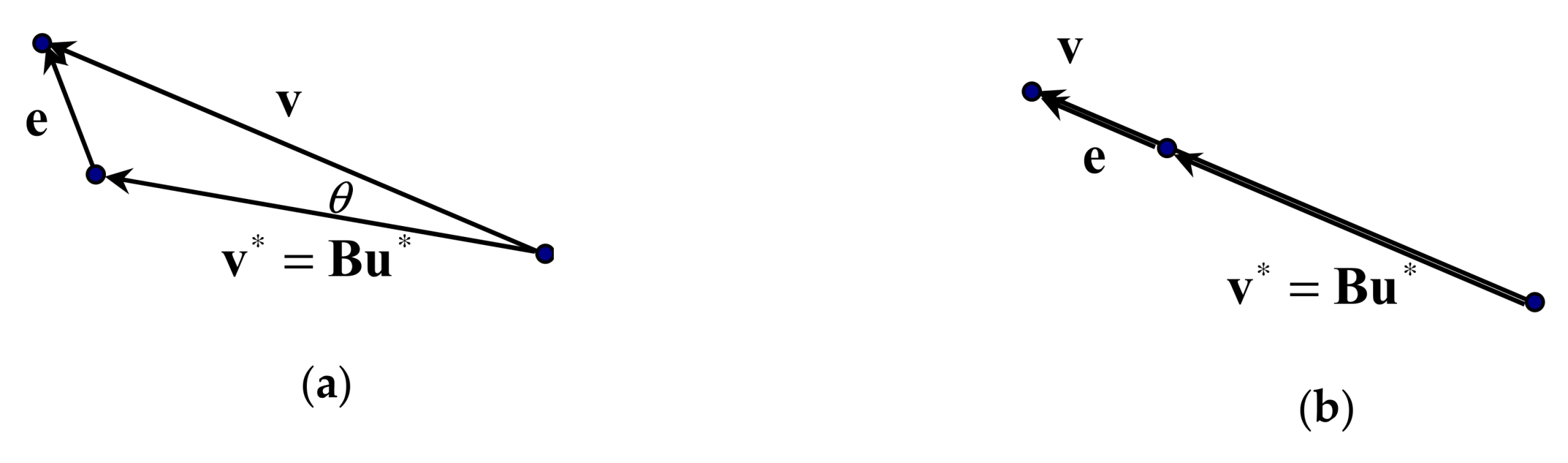
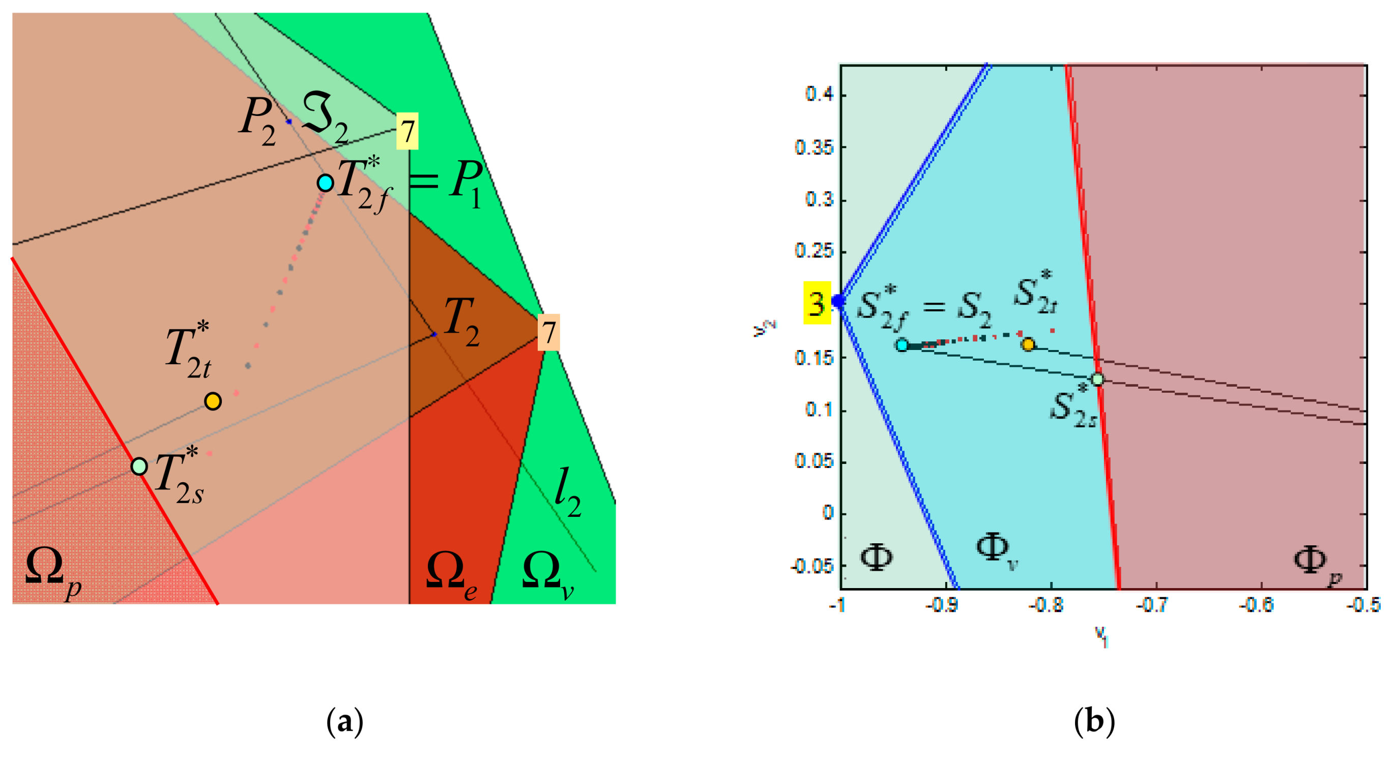
- T-approximation of the unfeasible pseudoinverse solution, introduces direction error , i.e., vectors and have not the same direction. At the same time, the direction error for S-approximation , i.e., vectors and always have the same direction, but the magnitude error is greater than .
- The fixed-point method (Section 3.3) is able to improve the T- or S-approximation of the unfeasible weighted pseudoinverse solution . Approximations or can be used as the initial iteration and the algorithm will find the solution such that is a better approximation of than or . This feature is the main idea of the hybrid approach for control allocation.
3.3. Fixed-Point Method
Introduction
3.4. Algorithm (Hybrid Method)
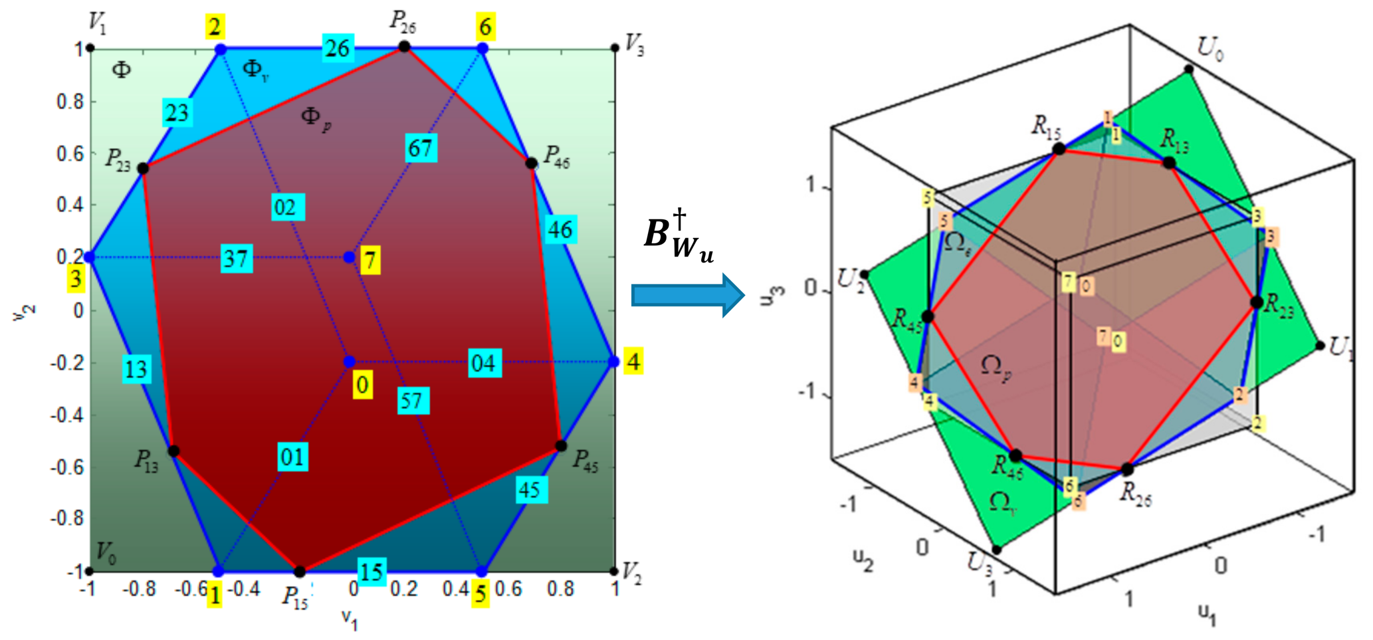
3.5. Extension of Concepts from “virtual” ROV to Open-Frame ROV
- If lies inside , then has an infinite number of points, and the control allocation problem has an infinite number of solutions.
- If lies on the boundary of , then is a single point, the unique solution for the control allocation problem.
- If lies outside , then is an empty set, i.e., no exact solution exists, only approximation.
4. Testing and Validation
4.1. Evaluation of the FTC in Virtual Environment
4.1.1. Partial Fault in HT2
4.1.2. Total Fault in HT2
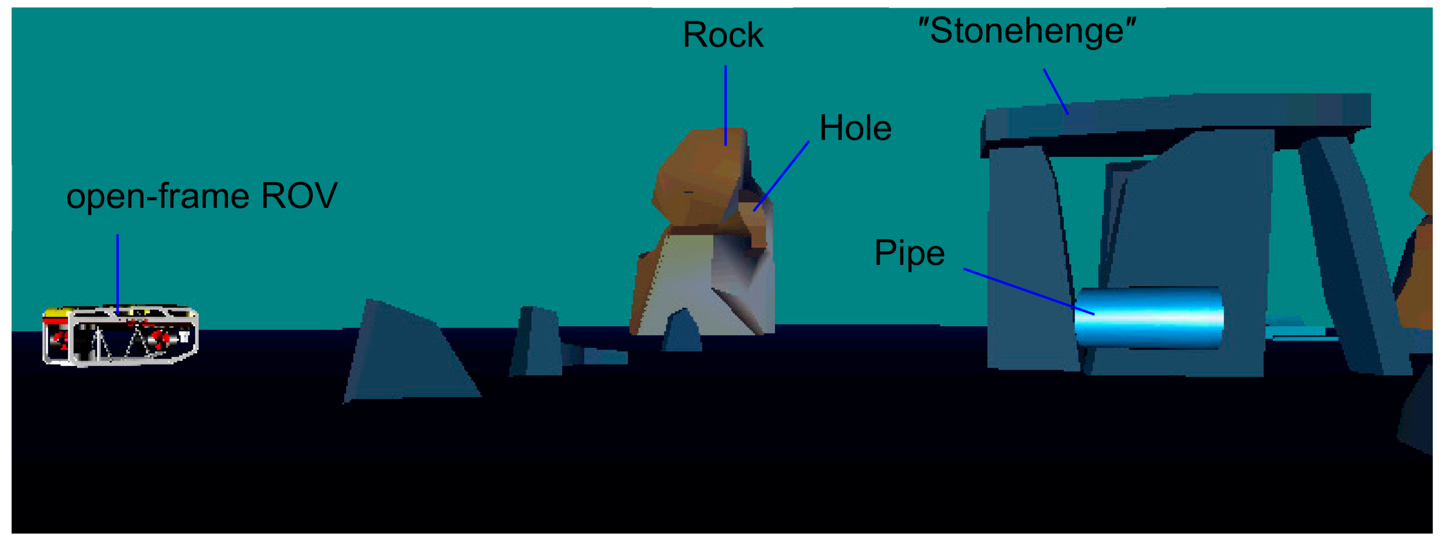
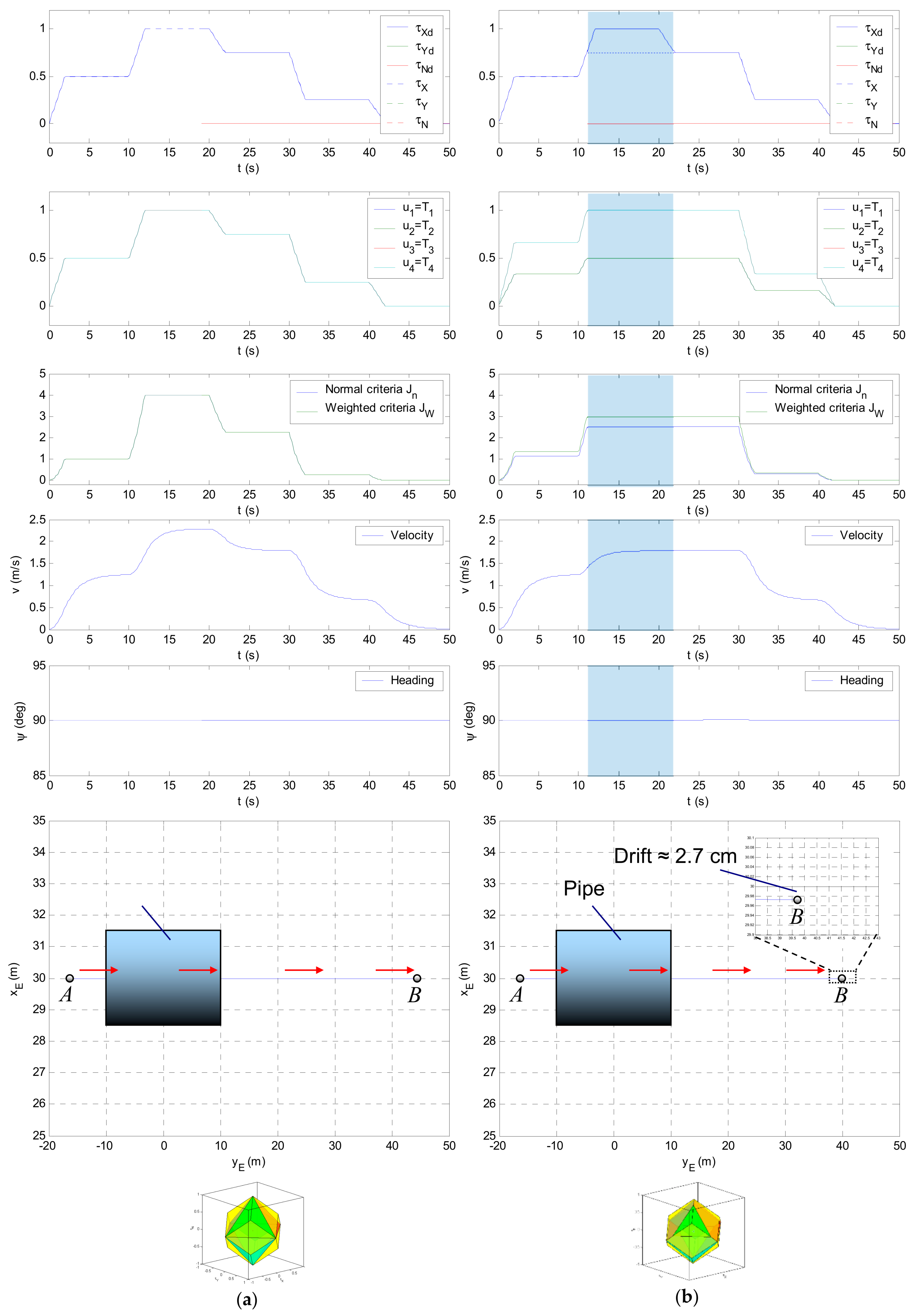
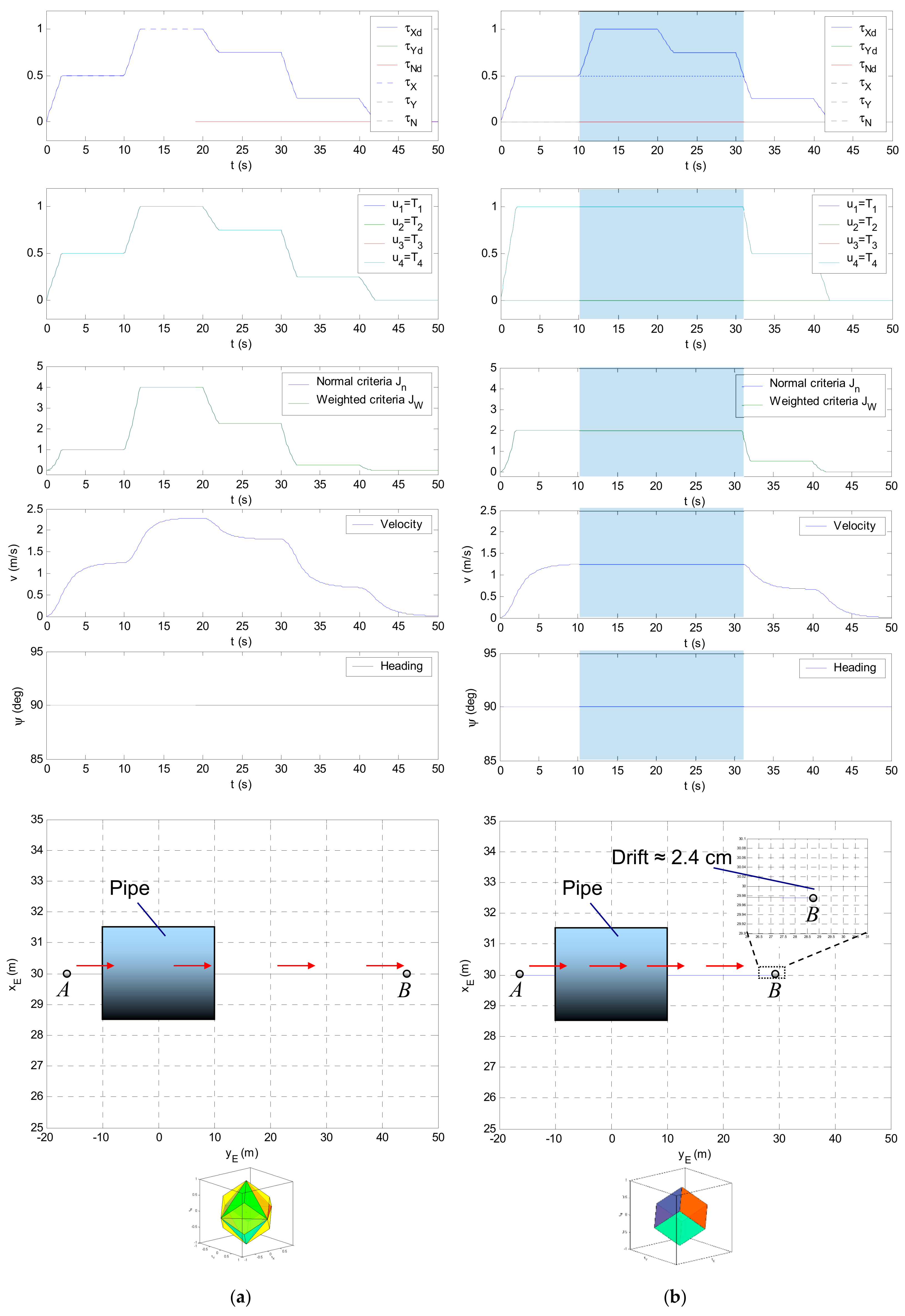
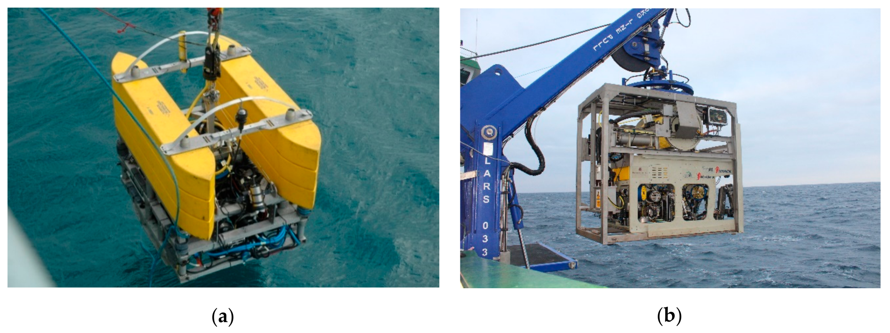
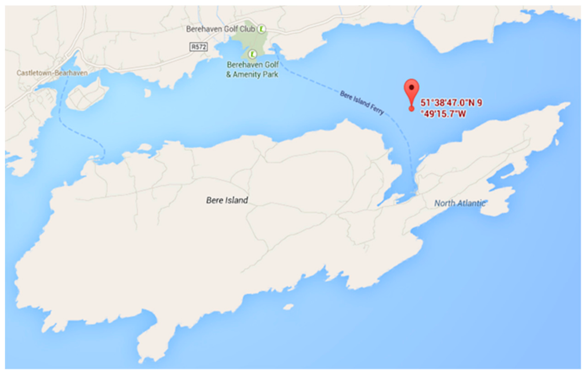
4.2. Evaluation of the FTC in Real-World Environment
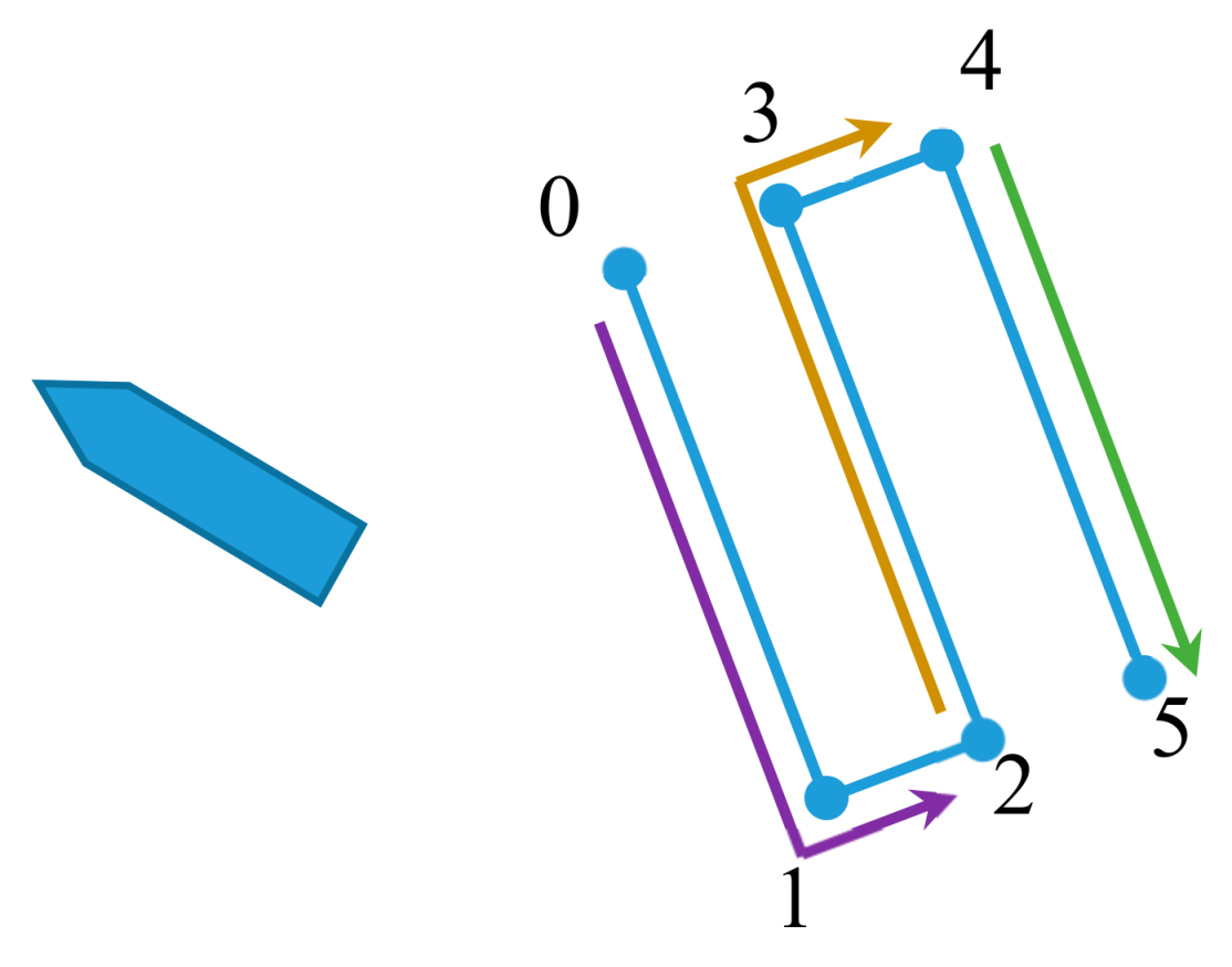
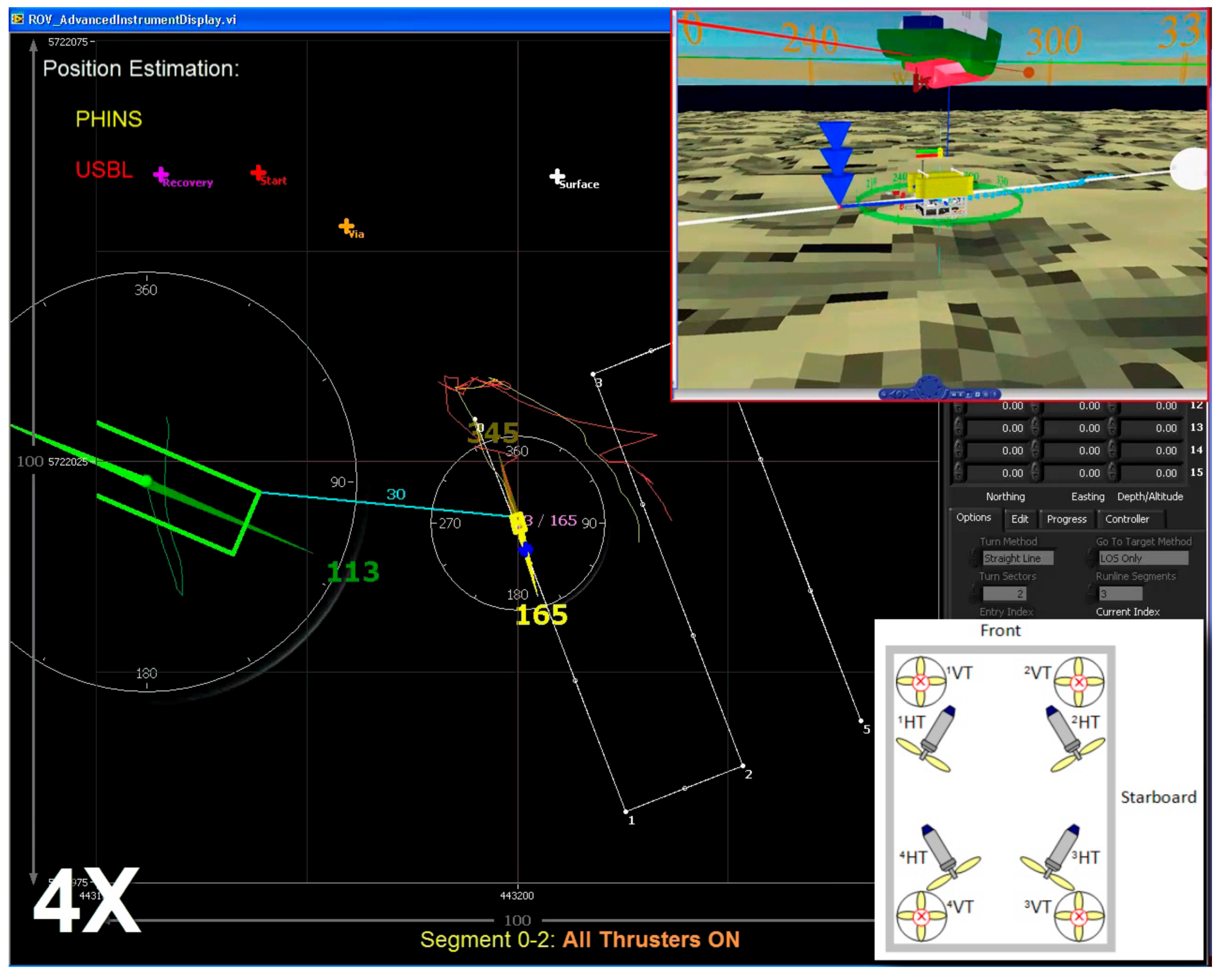
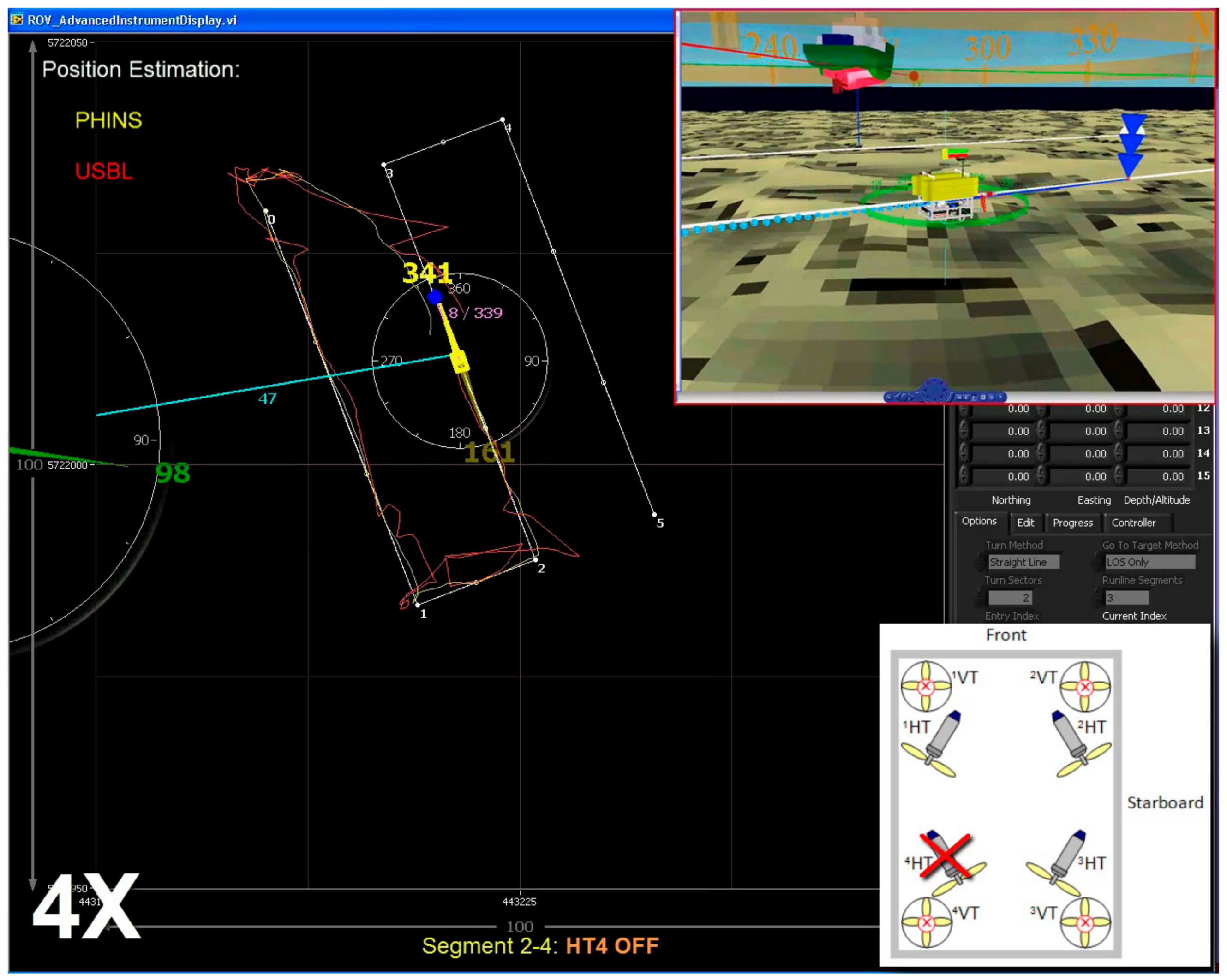
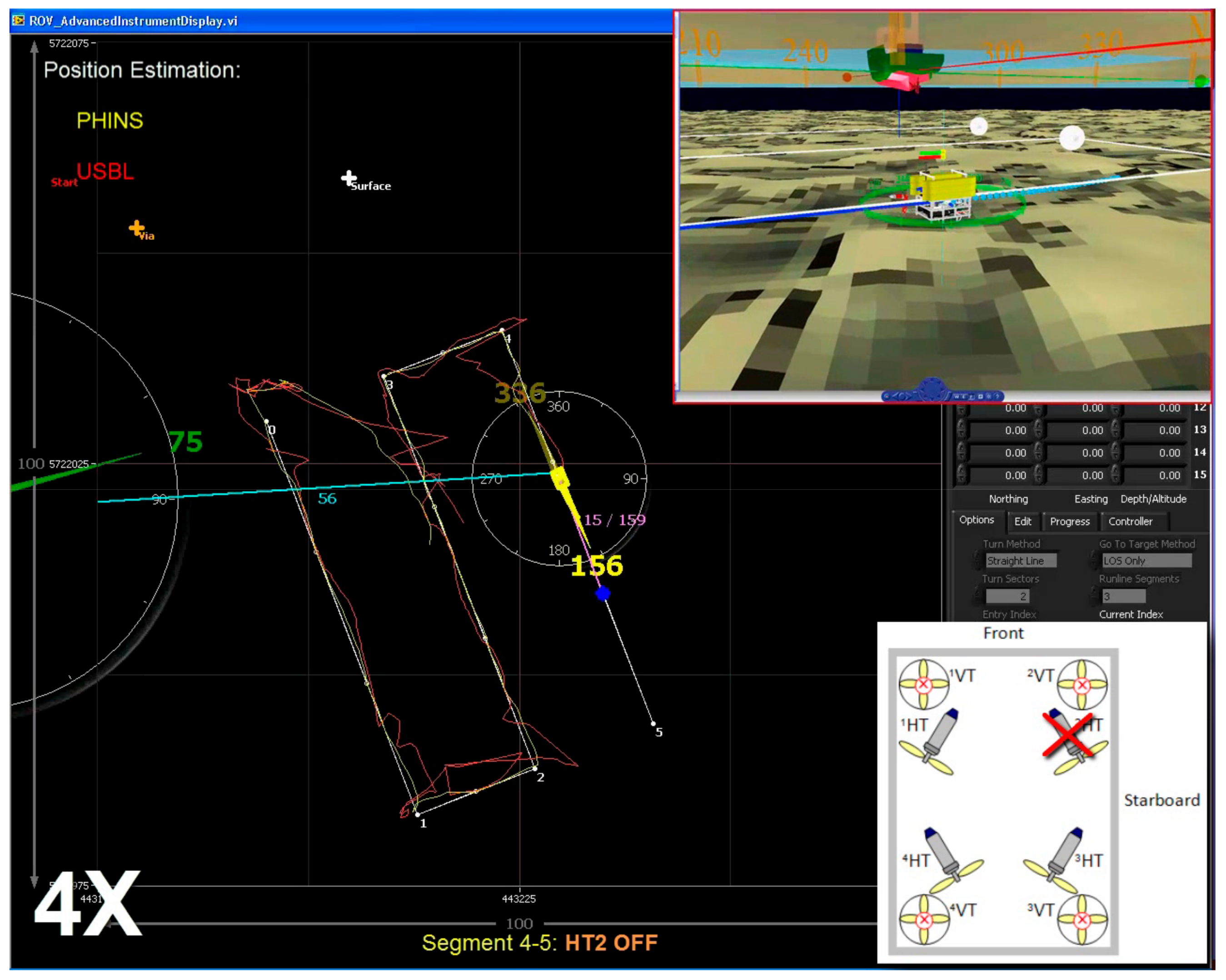
4.2.1. Path Following: Simulated Faults
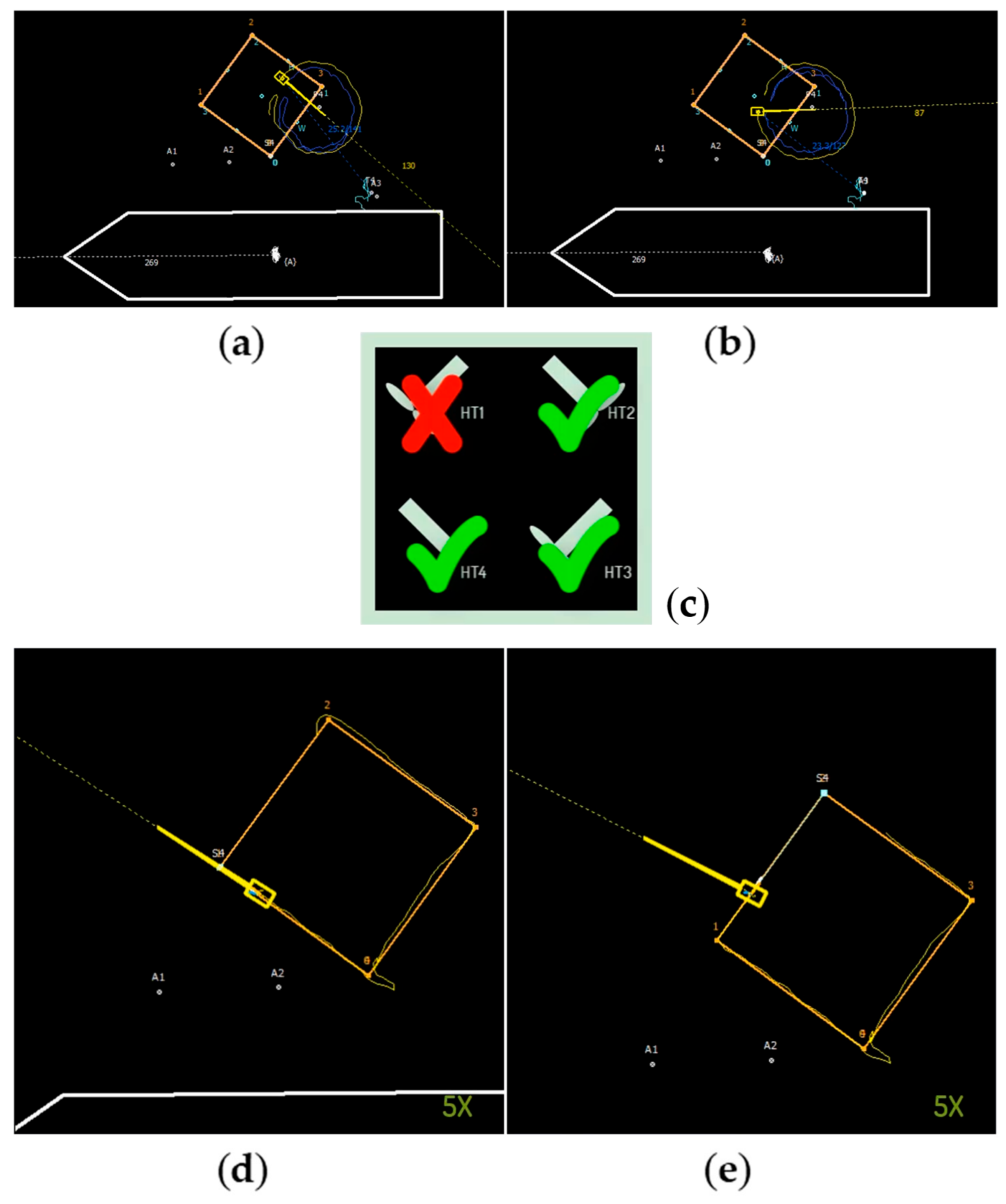
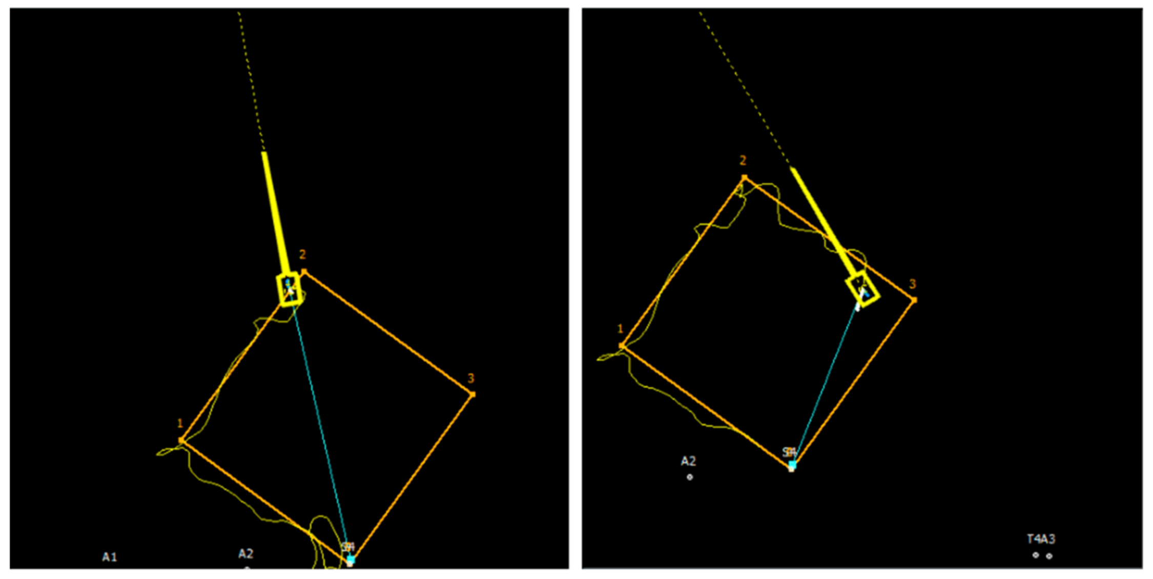
4.2.2. Complex Tasks with Faulty Thruster
5. Conclusions
Author Contributions
Funding
Conflicts of Interest
References
- Blanke, M.; Kinnaert, M.; Lunze, J.; Staroswiecki, M. Diagnosis and Fault-Tolerant Control; Springer: Berlin/Heidelberg, Germany, 2006; ISBN-13 978-3-540-35652-3. [Google Scholar]
- Oppenheimer, M.; Doman, D.; Bolender, M. Control allocation. In The Control Handbook, Control System Applications, 2nd ed.; Levine, W.S., Ed.; CRC Press: Boca Raton, FL, USA, 2010; Chapter 8. [Google Scholar]
- Fossen, T.I.; Johansen, T.A. A survey of control allocation methods for ships and underwater vehicles. In Proceedings of the 14th Mediterranean Conference on Control and Automation, Ancona, Italy, 28–30 June 2006. [Google Scholar]
- Johansen, T.A.; Fossen, T.I. Control allocation—A survey. Automatica 2013, 49, 1087–1103. [Google Scholar] [CrossRef] [Green Version]
- Zhang, Y.; Zeng, J.; Li, Y.; Sun, Y.; Wan, L.; Huang, S. Research on reconstructive fault-tolerant control of an X-rudder AUV. In Proceedings of the OCEANS 2016 MTS/IEEE Monterey, Monterey, CA, USA, 19–23 September 2016. [Google Scholar]
- Chu, Z.; Luo, C.; Zhu, D. Adaptive fault-tolerant control for a class of remotely operated vehicles under thruster redundancy. In Proceedings of the IEEE 8th International Conference on Underwater System Technology: Theory and Applications (USYS), Wuhan, China, 1–3 December 2018. [Google Scholar] [CrossRef]
- Liu, X.; Zhang, M.; Yao, F. Adaptive fault-tolerant control and thruster fault reconstruction for an autonomous underwater vehicle. Ocean Eng. 2018, 155, 10–23. [Google Scholar] [CrossRef]
- Ropars, B.; Lasbouygues, A.; Lapierre, L.; Andreu, D. Thruster’s dead-zones compensation for the actuation system of an underwater vehicle. In Proceedings of the European Control Conference (ECC), Linz, Austria, 15–17 July 2015; pp. 741–746. [Google Scholar]
- Baldini, A.; Ciabattoni, L.; Felicetti, R.; Ferracuti, F.; Freddi, A.; and Monteriù, A. Dynamic surface fault-tolerant control for underwater remotely operated vehicles. ISA Trans. 2018, 78, 10–20. [Google Scholar] [CrossRef]
- Chin, C.S.; Lau, M.W.S.; Low, E.; Seet, G.G.L. Design of Thrusters Configuration and Thrust Allocation Control for a Remotely Operated Vehicle. In Proceedings of the IEEE Conference on Robotics, Automation and Mechatronics, Bangkok, Thailand, 1–3 June 2006. [Google Scholar] [CrossRef]
- De Carolis, V.; Maurelli, F.; Brown, K.E.; Lane, D.M. Energy-aware fault-mitigation architecture for underwater vehicles. Auton. Robot. 2017, 41, 1083–1105. [Google Scholar] [CrossRef]
- Davoodi, M.; Meskin, N.; Khorasani, K. Event-triggered fault estimation and accommodation design for linear systems. In Proceedings of the Second International Conference on Event-based Control, Communication, and Signal Processing (EBCCSP), Krakow, Poland, 13–15 June 2016. [Google Scholar]
- Karras, G.C.; Fourlas, G.K. Model Predictive Fault Tolerant Control for Omni-direct ional Mobile Robots. J. Intell. Robot. Syst. 2019. [Google Scholar] [CrossRef]
- Liu, H.; Wei, Y.; Zhou, X.; Li, G. Operated ROV Thrust Distribution Control System Based on Adaptive Back-stepping controller. In Proceedings of the 35th Chinese Control Conference, Chengdu, China, 27–29 July 2016. [Google Scholar]
- Antonelli, G.; Fossen, T.I.; Yoerger, D.R. Underwater Robotics. In Springer Handbook of Robotics; Siciliano, B., Khatib, O., Eds.; Springer: Berlin/Heidelberg, Germany, 2008; pp. 987–1008. [Google Scholar]
- Antonelli, G. Underwater Robots, 2nd ed.; STAR 2; Springer: Berlin/Heidelberg, Germany, 2006; pp. 79–91. [Google Scholar]
- Omerdic, E.; Roberts, G.N. Thruster fault diagnosis and accommodation for open-frame underwater vehicles. Control Eng. Pract. 2004, 12, 1575–1598. [Google Scholar] [CrossRef]
- Fossen, T.I. Handbook of Marine Craft Hydrodynamics and Motion Control; John Wiley & Sons: Hoboken, NJ, USA, 2011. [Google Scholar]
- Härkegârd, O. Backstepping and Control Allocation with Application to Flight Control. Ph.D. Thesis, Department of Electrical Engineering, Linköping University, Linköping, Sweden, 2003. [Google Scholar]
- Omerdic, E. Thruster Fault-Tolerant Control; VDM Verlag: Riga, Latvia, 2009; ISBN 978-3-639-11739-4. [Google Scholar]
- Bodson, M. Evaluation of Optimisation Methods for Control Allocation. J. Guid. Control Dyn. 2002, 25, 703–711. [Google Scholar] [CrossRef]
- Burken, J.; Lu, P.; Wu, Z.; Bahm, C. Two Reconfigurable Flight-Control Design Methods: Robust Servomechanism and Control Allocation. J. Guid. Control Dyn. 2001, 24, 482–493. [Google Scholar] [CrossRef] [Green Version]
- Omerdic, E.; Toal, D.; Nolan, S.; Ahmad, H. ROV LATIS: Next Generation Smart Underwater Vehicle. In IET Book: Further Advances in Unmanned Marine Vehicles; Inst of Engineering & Technology: London, UK, 2002; Chapter 2; ISBN-10 1849194793, ISBN-13 978-1849194792. [Google Scholar]


| Virtual Control Input | ||||
|---|---|---|---|---|
| —Surge Force —Sway Force —Yaw Moment | —Heave Force —Roll Moment —Pitch Moment | |||
| Virtual ROV | Open-Frame ROV | |
|---|---|---|
| Virtual Control Input | ||
| True Control Input | ||
| Control Effectiveness Matrix | ||
| Actuator Position Constraints | ||
| Control Allocation Problem (Inequalities (2) and (4) apply component-wise.) | For a given , find such that | For a given , find such that |
| −0.7917 | 0.7917 | −0.6875 | 0.6875 | −0.2000 | 0.2000 | |
| 0.5333 | −0.5333 | −0.5500 | 0.5500 | −1.0000 | 1.0000 |
| −1.0000 | 1.0000 | −1.0000 | 1.0000 | −0.4000 | 0.4000 | |
| 1.0000 | −1.0000 | −0.2500 | 0.2500 | −1.0000 | 1.0000 | |
| 0.1667 | −0.1667 | 1.0000 | −1.0000 | 1.0000 | −1.0000 |
| Virtual Control Space | True Control Space | ||
|---|---|---|---|
| Partition | Polygon | Partition | Polygon |
| Initial Point | # Of Iterations | Last Iteration | Limit | Obtained Virtual Control Input | Desired Virtual Control Input | Direction Error | Magnitude Error |
|---|---|---|---|---|---|---|---|
| 19 | |||||||
| 20 |
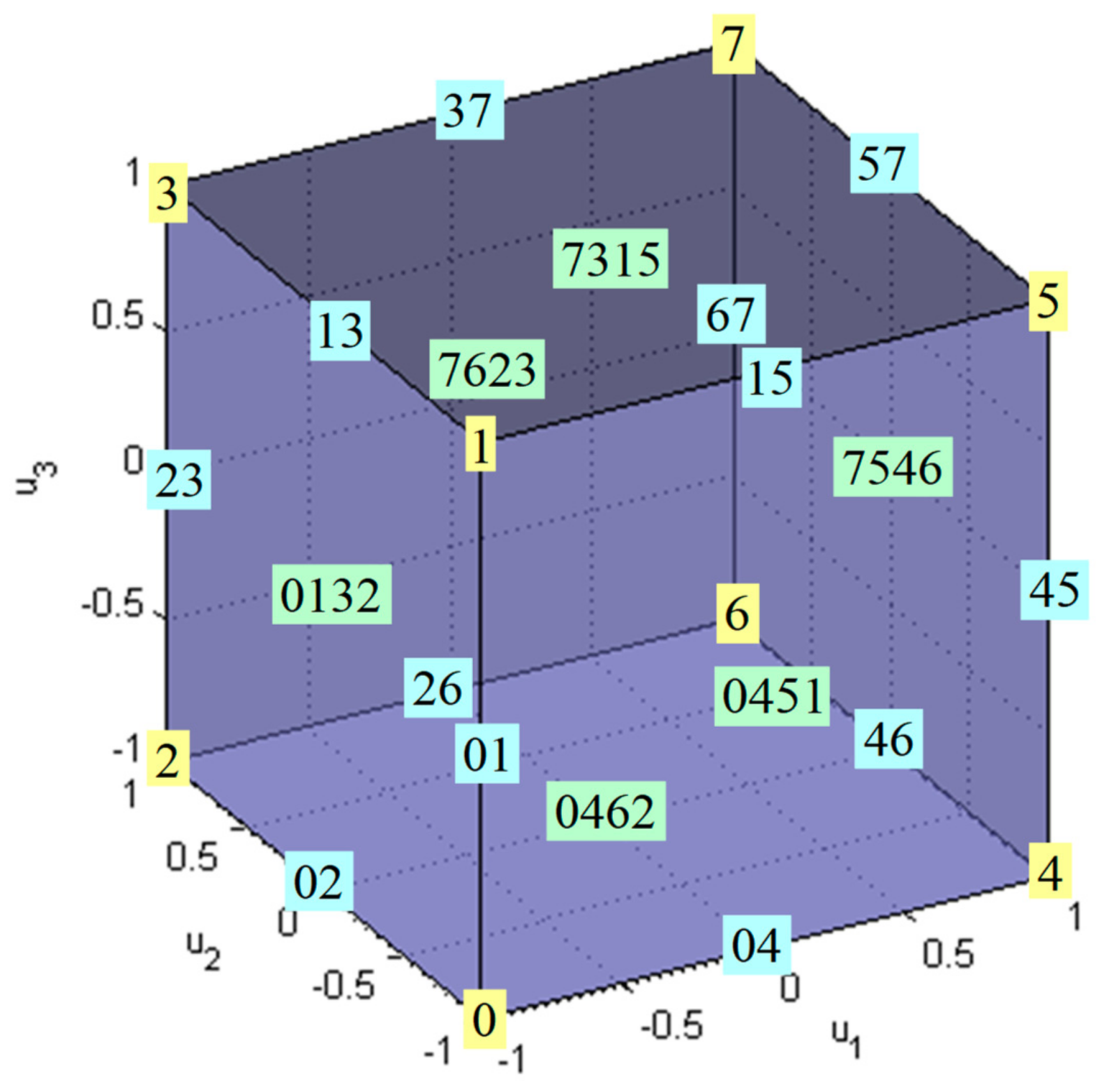
| Label | Coordinates | Label | Coordinates | |||||
|---|---|---|---|---|---|---|---|---|
| 0 | −1 | −1 | −1 | −1 | 0 | −1.0 | 0.0 | 0.0 |
| 1 | −1 | −1 | −1 | +1 | 1 | −0.5 | −0.5 | 0.5 |
| 2 | −1 | −1 | +1 | −1 | 2 | −0.5 | 0.5 | −0.5 |
| 3 | −1 | −1 | +1 | +1 | 3 | 0.0 | 0.0 | 0.0 |
| 4 | −1 | +1 | −1 | −1 | 4 | −0.5 | −0.5 | −0.5 |
| 5 | −1 | +1 | −1 | +1 | 5 | 0.0 | −1.0 | 0.0 |
| 6 | −1 | +1 | +1 | −1 | 6 | 0.0 | 0.0 | −1.0 |
| 7 | −1 | +1 | +1 | +1 | 7 | 0.5 | −0.5 | −0.5 |
| 8 | +1 | −1 | −1 | −1 | 8 | −0.5 | 0.5 | 0.5 |
| 9 | +1 | −1 | −1 | +1 | 9 | 0.0 | 0.0 | 1.0 |
| A | +1 | −1 | +1 | −1 | A | 0.0 | 1.0 | 0.0 |
| B | +1 | −1 | +1 | +1 | B | 0.5 | 0.5 | 0.5 |
| C | +1 | +1 | −1 | −1 | C | 0.0 | 0.0 | 0.0 |
| D | +1 | +1 | −1 | +1 | D | 0.5 | −0.5 | 0.5 |
| E | +1 | +1 | +1 | −1 | E | 0.5 | 0.5 | −0.5 |
| F | +1 | +1 | +1 | +1 | F | 1.0 | 0.0 | 0.0 |
| Segment | HT1 | HT2 | HT3 | HT4 |
|---|---|---|---|---|
| 01 | ON | ON | ON | ON |
| 12 | ON | ON | ON | ON |
| 23 | ON | ON | ON | OFF |
| 34 | ON | ON | ON | OFF |
| 45 | ON | OFF | ON | ON |
© 2020 by the authors. Licensee MDPI, Basel, Switzerland. This article is an open access article distributed under the terms and conditions of the Creative Commons Attribution (CC BY) license (http://creativecommons.org/licenses/by/4.0/).
Share and Cite
Omerdic, E.; Trslic, P.; Kaknjo, A.; Weir, A.; Rao, M.; Dooly, G.; Toal, D. Geometric Insight into the Control Allocation Problem for Open-Frame ROVs and Visualisation of Solution. Robotics 2020, 9, 7. https://doi.org/10.3390/robotics9010007
Omerdic E, Trslic P, Kaknjo A, Weir A, Rao M, Dooly G, Toal D. Geometric Insight into the Control Allocation Problem for Open-Frame ROVs and Visualisation of Solution. Robotics. 2020; 9(1):7. https://doi.org/10.3390/robotics9010007
Chicago/Turabian StyleOmerdic, Edin, Petar Trslic, Admir Kaknjo, Anthony Weir, Muzaffar Rao, Gerard Dooly, and Daniel Toal. 2020. "Geometric Insight into the Control Allocation Problem for Open-Frame ROVs and Visualisation of Solution" Robotics 9, no. 1: 7. https://doi.org/10.3390/robotics9010007