
Design and Control of the Rehab-Exos, a Joint Torque-Controlled Upper Limb Exoskeleton †
by
 , , and
Domenico Chiaradia
1,*,
Gianluca Rinaldi
1,
Massimiliano Solazzi
1,
Rocco Vertechy
2 and
Antonio Frisoli
1 1
Institute of Mechanical Intelligence and Department of Excellence in Robotics & AI, Scuola Superiore Sant’Anna, 56127 Pisa, Italy
2
DIN—Department of Industrial Engineering, University of Bologna, 40136 Bologna, Italy
*
Author to whom correspondence should be addressed.
†
This paper is an extended version of our paper published in Solazzi, M.; Abbrescia, M.; Vertechy, R.; Loconsole, C.; Bevilacqua, V.; Frisoli, A. An interaction torque control improving human force estimation of the rehab-exos exoskeleton. In Proceedings of the 2014 IEEE Haptics Symposium (HAPTICS), Houston, TX, USA, 23–26 February 2014; pp. 187–193.
Robotics 2024, 13(2), 32; https://doi.org/10.3390/robotics13020032
Submission received: 3 January 2024
/
Revised: 12 February 2024
/
Accepted: 15 February 2024
/
Published: 17 February 2024
(This article belongs to the Special Issue AI for Robotic Exoskeletons and Prostheses)
Abstract
:This work presents the design of the Rehab-Exos, a novel upper limb exoskeleton designed for rehabilitation purposes. It is equipped with high-reduction-ratio actuators and compact elastic joints to obtain torque sensors based on strain gauges. In this study, we address the torque sensor performances and the design aspects that could cause unwanted non-axial moment load crosstalk. Moreover, a new full-state feedback torque controller is designed by modeling the multi-DOF, non-linear system dynamics and providing compensation for non-linear effects such as friction and gravity. To assess the proposed upper limb exoskeleton in terms of both control system performances and mechanical structure validation, the full-state feedback controller was compared with two other benchmark-state feedback controllers in both a transparency test—ten subjects, two reference speeds—and a haptic rendering evaluation. Both of the experiments were representative of the intended purpose of the device, i.e., physical interaction with patients affected by limited motion skills. In all experimental conditions, our proposed joint torque controller achieved higher performances, providing transparency to the joints and asserting the feasibility of the exoskeleton for assistive applications.
1. Introduction
Exoskeletons are robotic interfaces for human–robot interaction where the highest physical symbiosis with the human operator is achieved. Unlike many industrial robots designed to exhibit a rigid structure and behavior, to be used with a stiff position control, exoskeletons are designed to satisfy compliance and safety requirements commonly employed by physical human–robot interaction (pHRI) devices [1]. Other performance metrics, inherently depending on actuation and control systems, need to be taken into account when designing an exoskeleton whose main purpose is to provide assistance to patients in need of rehabilitation treatments. An assistive device must be able to support the weight of any impaired limbs of the patient as well as provide sufficient forces to allow the correct completion of the task [2].
Therefore, two of the most relevant metrics for evaluating an assistive device are as follows:
- Transparency: It relates to the ability of the robotic system to not apply any resistance to free motion when interacting with a human user who is moving voluntarily [3], or, equivalently, it means that the robot’s reaction forces perceived by the user are minimal [4]. Although no standard procedures exist for measuring transparency in pHRI, there is a general consensus in the exoskeletons field to refer not only to end effector resistance forces but also to single-joint resistance torques or measurements coming from specific contact points [4];
- Haptic rendering: It refers to the device’s capability to render a desired dynamic behavior such as a virtual impedance or a virtual wall, i.e., a task featuring both very high impedance—when in contact with the wall—and very low impedance—when out of contact [5]. An efficient mechanical structure should be able to predict the maximum stiffness displayed by existing devices by including appropriate dimensioning of sensors and actuators combined with more effective control strategies [6].
In the last two decades, several exoskeleton prototypes have been proposed using different implementation principles depending on the field of application [2], such as neuro-rehabilitation and assistance [7,8,9,10], human power augmentation [11] and telepresence [12,13,14]. The majority of exoskeletons employed in the aforementioned fields—especially for rehabilitation purposes—are active, which means they employ an actuation system capable of actively providing and transmitting the required force to the human user. There are many types of actuator systems, each one employing different solutions for power transmission, such as geared actuators [15,16], tendon drives [17,18], hybrid solutions [19,20] and pneumatic or hydraulic systems [21,22,23]. According to how each actuation system adjusts the impedance displayed to the user, it is possible to classify the actuators employed in pHRI into two main categories, as shown in Figure 1a. There are actuation systems with active impedance by control— i.e., they render impedance by the means of a control system—which mainly rely on position and torque sensors, and others that present inherent impedance—i.e., the impedance is obtained by inherent mechanical properties of the actuator—such as compliance or damping [24].
Actuators employing inherent compliance provide an electric motor coupled with a spring. Depending on whether the spring is fixed—i.e., its value does not change—like mechanical springs, or variable like silicone rubber springs, these actuators can be classified respectively into Series Elastic Actuators (SEAs) and Variable-Stiffness Actuators (VSAs). Both of the solutions are based on the principle that, by adding a series elastic element between load and actuator, it is possible to reduce the peak power requested from the motor. Inherent damping actuators are based on the control of friction by means of eddy currents, controlled rheology or fluid dynamics. Both SEAs and VSAs have been implemented in exoskeletons such as Lopes [25], the NEUROexos elbow exoskeleton [26], the ALTACRO locomotion exoskeleton [27] and the Harmony exoskeleton [28]. These actuators have the great advantage of impact absorption, thus enhancing the system safety. Moreover, SEAs and VSAs are eventually capable of mechanically storing energy during passive phases while releasing it in active phases of the motion cycle. VSAs generally employ two motors, which increase the size, weight and complexity of the whole actuator in comparison with an SEA [29].
On the other side, actuators employing active impedance by control are equipped with electric motors coupled with a transmission/reduction system; they can be classified according to the back-drivability and sensing system. Force-controlled actuators implement a force/torque sensor at the joint level, and they can achieve impedance behavior by closed-loop control. Generally, traditional actuators with no elastic or damping elements are lighter and more compact than passive variable impedance actuators, but their time response and dynamic bandwidth are limited by the control system as well as the electrical properties of actuators, such as motor maximum speed.
Simplified block diagrams of the solutions based on active impedance by control, an SEA and a VSA are reported in Figure 1b.
The majority of recent exoskeletons based on joint torque sensors have been mostly designed for lower limb solutions [30,31,32]. The main advantages of these systems are their compactness and robustness, though when the torque sensor is embedded in the joint, it becomes sensitive to the link inertia, thus affecting the system transparency. A mechanical solution is presented in Ref. [33], and the transparency of a lower limb exoskeleton is improved by positioning the force/torque sensor on the supporting cuffs, that is, at the interaction point between the human leg and the exoskeleton. Sensors generally employed to measure angular deflections are encoders [34] and potentiometers [35]—usually requiring custom mechanical supports to avoid errors related to sensitivity to misalignments. While deflection-based force estimation has become the most widely utilized method for SEAs and VSAs performing reliable force control in various robotic applications, there are still practical difficulties such as errors in spring deflection measurements or noise in the encoder signal [36]. These factors have a very negative impact on high-stiffness SEAs. In [37], a polymer optical fiber is mounted on the torsional spring of an SEA to read angles and torques in a more accurate way without considerably enlarging the actuator size at the cost of more specific (and complex) electronics.
Therefore, the adoption of inherent compliant actuation systems rather than achieving compliance by control is not a trivial choice; it mainly depends on the desired mechanical features, and it is the result of a trade-off among many factors such as compactness and weight, costs, safety and efficiency. The mentioned advantages and disadvantages of the SEA, VSA and active impedance by control solutions are summarized in Table 1.
In this paper, we propose a solution based on active impedance obtained by closed-loop control employing an elastic component to measure and transmit axial torques at the same time. This is a good trade-off favoring compactness and simplicity using just one motor. We implement a joint torque controller based on novel full-state feedback (JTFC1) to obtain a short time response and a high dynamic bandwidth by closed-loop control to achieve a desired impedance behavior.
The design of a closed-loop feedback torque control is an essential aid for managing the identification of human intention in pHRI [2]. Among the broad variety of force/torque controllers available in the literature, and, particularly, among the ones based on direct joint torque sensor readings, Hashimoto et al. proposed a single-joint torque controller based on torque readings estimated from the harmonic drive elasticity [38]. The basic closed-loop controller was tested with different feedforward compensation terms in order to achieve high disturbance reduction and robustness to model error. Moreover, Kugi et al. proposed a passivity-based impedance controller configuration, providing an inner torque feedback loop based on joint torque readings in combination with an outer impedance control loop [39]. This controller configuration was tested with the DLR Light Weight Robot III (LWR III) in several experiments which verified the efficiency of this approach. Both of these aforementioned control approaches have the common goal of providing safe and efficient pHRI by designing a closed-loop controller able to compensate non-linear effects as well as offering accurate estimation of the interaction forces.
Moreover, in this paper, we introduce the design and the experimental characterization of the Rehab-Exos, an upper limb exoskeleton designed for rehabilitation purposes and equipped with actuators based on joint torque sensors and a high reduction ratio. We contribute by designing a joint torque controller based on novel full-state feedback (JTFC1) that takes into account the multi-DOF, non-linear system dynamics and provides compensation for other non-linear effects such as friction and gravity components. This is accomplished by employing a single-joint optimum observer that ensures joint torque tracking while a centralized controller estimates and compensates for the whole system’s dynamics. To validate the proposed controller for the Rehab-Exos, in both transparency and haptic rendering experiments, the full-state feedback controller is compared with two alternative controllers: a feedback controller (JTFC2) inspired by Ref. [38] and a passivity-based feedback controller (JTFC3) inspired by Ref. [39]. The experiments performed with our proposed controller validate the Rehab-Exos as a device able to achieve satisfying pHRI performances, thus asserting the feasibility of the Rehab-Exos for human assistance and rehabilitation purposes.
This paper is structured as follows: Section 2 presents the design of the Rehab-Exos, with a particular focus on the design and issues related to its torque sensors based on strain gauges. Section 3.1 provides a mathematical model of the single joint, whereas, in Section 3.2, the full dynamics model of the Rehab-Exos is described. Section 4 explains the proposed full-state feedback controller and recalls two benchmark torque controllers already known from the literature. Section 5 presents the experiments and the obtained results. Finally, discussions and conclusions are respectively addressed in Section 6 and Section 7.
2. System Design
The Rehab-Exos (Figure 2) is an active robotic exoskeleton designed to be modular and easily re-configurable. Since rehabilitation applications are its final purpose, it is designed to be capable of generating controlled contact forces/torques not only at its end effector handle but also at intermediate contact points with the human user’s arm. By wearing the device, the patient is able to control the full force interaction with the exoskeleton as well as guide—or be guided by—shoulder and elbow articulations. The joint torque sensors monitor the physical interaction between the user and the exoskeleton.
2.1. Mechanical Design of the Rehab-Exos
As depicted in Figure 2, the exoskeleton has a serial architecture which is isomorphic with human kinematics. It comprises a shoulder joint which is fixed in the space, and it is composed of three active joints, , and , an active elbow joint, , and a passive revolute joint, , allowing wrist prono/supination. For a more detailed description of both the Rehab-Exos and actuation groups, the reader can refer to Ref. [40]. The exoskeleton is grounded to a supporting structure that can be easily moved via passive wheels, and the height of the first link can be adjusted; thus, the position of the center of the shoulder of the exoskeleton can be set to fit the center of the shoulder of the user. The actuation stage of the joints , and of the exoskeleton is identical. These joints integrate a compact harmonic drive (HD) component set—which implements a high reduction ratio of 100:1—and a custom-made frame-less, brushless torque motor. The maximum joint output torque of the actuator is equal to 150 Nm with an overall weight of 3.7 kg and a motor shaft inertia, reduced to the joint output shaft , equal to 2.5 kgm2. The adopted mechanical components limit both the back-drivability—when the motor is powered off—and the overall mechanical complexity. Nevertheless, the user never holds the weight of the joints because the gravitational and dynamic contributions are modeled and provided by the torque controller. Then, the reaction torques/forces to the first link are exerted by the supporting structure.
2.2. Design Aspects of the Strain-Gauge-Based Torque Sensor
The three joints , and have a torque sensor featuring a four-spoke shape geometry. Despite increasing the actuation group compliance, the embedded torque sensors enable multi-contact force control. Moreover, it allows the implementation of a stable, high-bandwidth torque closed loop around each joint that is weakly affected by the variable inertia of the robot links; suppresses robot vibrations produced by the inherent transmission compliance (harmonic drive); reduces internal disturbance torques caused by the actuator and reducer as, for example, friction losses, actuators torque ripples and gear-teeth-wedging actions; and measures externally applied forces/moments and complex non-linear dynamic interactions between joints and links.
Each sensor embeds two fully balanced strain gauge bridges, located on different beams of the spoke. The sensor is made of AISI 630 steel, a harmonic steel exhibiting a yield strength of 1950 MPa and a Young’s modulus of 196 GPa, and it is designed to exhibit low weight and high sensitivity to axial moments. The axial torsional stiffness of the sensor is equal to 30 KNm/rad, and it can be computed as in Equation (1).
where the adimensional parameter Q is given by the following:
where, according to Figure 2d, r is the radius of the internal sensor ring, L is length of the beams and a is the side length of the beam section. The characteristic dimensions of the sensor are reported in Table 2. Moreover, the torsional stiffness of the joint reduced to its output shaft k is equal to 11.38 KNm/rad.
The position of the strain gauges on the beam is selected according to a trade-off process. By locating them in the middle of the beam, the sensor sensitivity is low, while locating them near the extremities of the beam results in sensor readings being affected by the non-linearities coming from the beam fillets. Taking this into account, the selected distances from the extremities are selected as and mm. To estimate the strain of the beam at a given point with distance p from the inner ring under a certain axial torque , the normal tension that acts on that point p needs to be computed as follows:
and then the strain is computed as follows:
where E is the Young’s modulus.
Theoretically, i.e., using (4), at 3 mm from the inner ring and under an axial torque of 120 Nm, a maximum strain of is obtained. The same test is conducted using an FEM software tool (Ansys® v.2019 R3.0) because the surface of the strain gauge is not negligible compared to the beam one (see Figure 3). The FEM analysis results in a maximum strain of . The strain of each strain gauge when a 1 Nm load is applied is shown in Table 3.
An important feature of the torque sensor is represented by the sensitivity to non-axial moments. For this reason, an experimental test is conducted to compute the sensitivity, i.e., predetermined non-axial torque is exerted on the sensor in four configurations (angles) of the sensor. Experimental results are reported in Table 4, and the obtained sensitivity is equal to the following:
Observing the results in Table 4, it should be noted that the sensitivity to non-axial moments is relatively high if compared to the one mentioned in Ref. [41]. The issue is investigated according to the steps reported in the roadmap of Figure 4. Indeed, the correct estimation of the joint torque is crucial for obtaining a high level of transparency of the controlled exoskeleton in all the poses of the workspace. To explain the experimental evidence, two possible reasons (or a combination of them) are proposed: the first cause of error could be represented by a strain gauge mounting misalignment; the second one could be related to an excessive deformation of the sensor due to the non-axial moments. Considering the first hypothesis of error, the sensitivity of the strain gauges to non-axial load due to strain gauge misalignment—when a flexible model of the HD is considered—can be modeled as follows:
where is a scaling factor equal to , is the sensitivity to linear mounting misalignment, which is equal to 3, and is the sensitivity to angular mounting misalignment and is equal to , whereas and are the positional and angular misalignment errors, respectively—see Figure 3a. Equation (6), together with the measured sensitivity of 0.067, leads to a misalignment error of millimeters and tens of degrees, but these values are higher than the actual misalignment the installation operator may have introduced, as can be seen in Figure 3b.
Regarding the second hypothesis, it is worth noticing that the sensor from a structural point of view is in series with the HD, and both of them are in parallel with a couple of bearings. This parallel chain composes a hyper-static system (see Figure 5); therefore, the excessive sensitivity may be due to the mounting misalignment of the mechanical parts of the chain.
For the study of the hyper-static system, the system parts are supposed to behave in a linear, elastic way, while the system response at non-axial moments is modeled as mono-dimensional. The overall joint stiffness to non-axial moment is experimentally evaluated, whereas the non-axial moment stiffness of the torque sensor and the HD are computed via FEM analysis. The FEM results are depicted in Figure 3, and the stiffness values are reported in Table 5.
A possible mounting misalignment of the hyper-static chain may consist of a collinear and/or concentric mounting misalignment between the sensor axis and the bearing axis. In this case, the HD works as a universal joint that connects the sensor—connected to the link—with the link. The sensitivity to non-axial moments defined in Equation (5) and the mechanical properties in Table 5 lead to a theoretical mounting misalignment of about 0.5 mm. However, this value does not agree with the design tolerances or the data-sheets of the components, from which a misalignment of about 0.05 mm is considered for the worst case.
To summarize, unwanted sensor readings related to non-axial load may be due to the combination of effects from sensor mounting misalignments and HD excessive deformation. In order to minimize this undesired effect, we adopt a model-free adaptive method based on Artificial Neural Networks (ANNs) to characterize and compensate this non-linear response of the sensors. This proposal represents an alternative method to modeling approaches, and the choice is justified by the complexity of the phenomenon.
Considering the ideal and linear response of the sensor, the torque readings can be expressed as follows:
where v is the measured voltage tension, and represents the voltage constant of the torque sensor. In a real case, it is possible to write the following:
where is the non-linear influence on the sensor readings due to the mounting and non-axial loads. By experimental evidence, it is possible to assert that the term varies in a non-linear way with respect to the exoskeleton pose (joint angles) and load. The mounting errors influence the torque readings in a non-linear way with respect to the joint angle, whereas the non-axial torques depend partially on the interaction with the human user and partially on the dynamics and gravitational torques acting on the considered joint. For all three sensors, the constants are experimentally evaluated. In order to minimize the effect of non-linear, undesired term , an ANN is involved in the process, with seven neurons in the hidden layer and sigmoid activation function. The goal is to estimate the error basing on the four angles and load on each axis. The angular information is useful for inferring the assembly error component, whereas, for the load influence, the gravitational torque is used. To train the neural network, the whole workspace is partitioned into 414 target points. The torque sensor readings are acquired while the exoskeleton is holding the target position. For each joint, the training is performed using the four angles and the gravity torque acting on the joint (and computed by the model) as input data, whereas the output is represented by the residual as follows:
where represents the gravity load on the i-th joint when the pose is given by the angle vector . The set of target points is divided into three parts: 70% for the training set, 20% for the validation set and 10% for the test set. The regression value between the ANN output and the target points is 0.99.
The actual sensor torque estimation is computed as follows:
2.3. Control Hardware
The control architecture of the Rehab-Exos is decentralized and based on the EtherCAT communication bus in order to guarantee both an optimal signal-to-noise ratio in the acquisition of analogical signals—i.e., the force sensors—and higher safety standards. The EtherCAT communication network consists of one master controller and four EtherCAT Slave Controllers (ESCs), one for each actuation joint. The master controller is handled by the Simulink Real-Time™ Operating System, which executes the centralized control model at 2 KHz of frequency. The exoskeleton is equipped with three 170 VDC power-supplied brushless motors on the first, second and fourth joint, each one driven by programmable current drivers, and one 48 VDC power-supplied DC motor on the third joint. Each motor is provided with one incremental encoder and one torque sensor. Each ESC board is a custom control board featuring an ARM7 micro-controller of up to 72 Mhz; four 14-bit DAC output interfaces setting the reference of the current drives; ten 14-bit Analog-to-Digital Converter (ADC) channels acquiring the torque signals through two pre-amplified Wheatstone full-bridge channels; and an EtherCAT ET1100 controller connecting to the double-port Ethernet interface.
3. Dynamic Model
3.1. Single-Joint Model
Each joint is modeled with a two-mass system with a spring and damper (Figure 6) due to the elasticity of the harmonic drive speed reducer and torque sensor for joints , and and due to the cable transmission for joint . The selected single-joint model is as follows.
The single-joint dynamics are represented by the following system of equations:
where, referring to the i-th joint, and represent the motor and joint angles, respectively; and are the stiffness and viscous coefficient of the transmission identified from experimental characterization; the terms and represent the inertia of the motor and the average link inertia considered as constant, respectively; and , and represent the torque of the motor, the disturbance torque acting on the motor rotor and the external torque acting directly on the output link, respectively. The term accounts for both the exogenous input due to the interaction with the human user and the endogenous input, which takes into account the unmodeled non-linear effects, such as dynamic or gravity forces.
Experimental Characterization of the Single Joint’s Performance
As described in Section 2.1, the joint is equipped with a torque sensor which is part of the transmission chain. It is also capable of measuring the elastic torque , which acts between the motor’s rotor and the joint output link. The elastic sensor torque can be expressed by the following:
The joint dynamics can be rewritten by putting in evidence of the readings starting from the definition then taking into account its first and second derivatives, as well as using Equations (11) and (12). As a result, the following equation is obtained:
where . The natural frequency of this system is computed as follows:
and it is experimentally evaluated for a single joint in a test rig by analyzing the response of the when a command torque signal of chirp type is fed to the motor.
From Figure 7, the use of the Half-Power Bandwidth method returns an overall damping coefficient c of the flexible joint equal to 11.8 Nms/rad. The obtained value is also validated via the Logarithmic Decrement method.
Each exoskeleton joint perceives link inertia depending on the pose; thus, the natural frequency of each joint depends on the pose of the exoskeleton. Therefore, the natural frequency for each joint elastic transmission can be obtained by taking into account average link inertia. Results are shown in Table 6.
The three joints referenced in Table 6 share the motor inertia value, which is equal to 3.742 kg/m2.
3.2. Multiple-Joints Model
Given the two-mass model employed for each single joint, the dynamic model of the whole exoskeleton can be formulated in matrix form as follows:
where , , , and are diagonal matrices; and represent, respectively, inertia and viscous friction at the motor; and represent stiffness and damping associated with the elastic transmission; represents the transmission reduction factor introduced by joint gear-heads; accounts for the gravity force effects on the links; and is the torques reflected on the joints due to the interaction forces exchanged between the human and the system where the transposed Jacobian matrix is evaluated in the actual exoskeleton configuration. The multi-joint model introduces cross-coupling among joints and non-linearities by taking into account the term , which is related to Coriolis effects, and the term , representing the links’ inertia. The latter term can be decomposed into a constant diagonal component and a variable one as follows:
By switching variables, this expression can also be introduced for the joint torque as follows:
Then, the dynamics Equation (16) can be rearranged, highlighting the new variables and as follows:
where the term represents the actual control command, while the external disturbance forces are collected within the external load force term —see Appendix A for a detailed derivation of terms.
From the reshaped dynamics equation, we define the full-state feedback control law and the optimal observer to estimate the joint torque.
3.2.1. Joint Acceleration Estimation
The full dynamics model of the exoskeleton is dependent on the acceleration of each joint. In order to estimate and compensate for the dynamics of the device, an observer for the joint acceleration is designed. The observer estimates the acceleration, taking into account the motor encoder readings , the joint torque and the commanded control torque . The term represents the torque measured by the sensor at the joint and can be expressed as in Equation (18). The acceleration can be estimated starting from a model of the actuation group—motor plus gear-head—and, additionally, by modeling the torque acting on the actuation group as and by considering the losses as a static and velocity-dependent viscous friction. Thus, the acceleration can be estimated as follows:
where the terms and represent the static friction torque and the dynamic friction, respectively, both of them previously experimentally evaluated. The torque saturation effects due to power supply voltage limits are modeled as follows:
depending on the electric constants of each motor. Particularly, where is the associated torque constant, the is the velocity constant, R is the winding terminal resistance and represents the maximum supply voltage to the motor.
An optimum observer is used to estimate the acceleration term . Figure 8 shows a diagram scheme of the acceleration estimator, which uses both controller and measured torques.
The model can be expressed in the state variable form as follows:
where
and represents the process noise.
The observer can be formulated as follows:
where L represents the gain matrix of the observer. A scheme of the observer is depicted in Figure 8.
The gain L is found, resolving the problem of the Kalman optimum observer based on the experimental covariance data of measurement and process noise. Measurement noise is derived from motor encoder readings , which mainly take into account the encoder quantization and motor acceleration estimate through (21) thanks to the available torque measurement.
As an example, the comparison between the real-time estimated acceleration—gray dotted line—and the off-line computed acceleration—black solid line—for the first two joints is shown in Figure 9.
3.2.2. Dynamics Compensation
As reported by Equation (A4), the torques measured by joint sensors relate to the human force and to any load applied on the links (). To obtain a good estimation of human forces by the torque sensors, it is necessary to remove the contributions of both gravity and dynamics loads applied to the links from torque measurements. The gravity contribution depends only on the pose of the exoskeleton, and it can be computed by the position signals acquired with the motor encoders. The gravitational term is already compensated in feedforward by the term in , except for the term . On the other side, the dynamics contribution depends on pose, velocity and acceleration of the links. These terms are not directly provided by any sensor, but they can be first approximated as by the observer described in Section 3.2.1.
The dynamic torques—which are generated from the links’ inertia and are measured by the joint torque sensors—can be estimated as the sum of the inertial contribution and the Coriolis effect as follows:
where matrices and are computed by taking into account for each joint the inertia of each part supported by the torque sensor while discarding the inertia of joint actuator.
The estimated dynamic torques are then used to compensate the dynamic effects of the link. The compensation torques , with , are a percentage of the estimated torques . The compensation torques are added to the desired torques as input to the state feedback controller and then fed back with the estimated torque .
4. Full-State, Basic and Passivity-Based Feedback Controllers
From the full dynamic model of the exoskeleton, a novel full-state feedback control law is derived and implemented where the state of the system is estimated through a Kalman filter algorithm—see Section 4.1. This control law is identified in the following with the acronym JTFC1 and explained in Section 4.2. To evaluate the performance of the proposed full-state feedback control, two other torque control methods are implemented. These two control methods are inspired by the existing joint torque controls available in the literature, and, in this work, they are addressed with the acronyms JTFC2 and JTFC3.
The JTFC2 controller—presented in Section 4.3—was first introduced by Hashimoto [38], and it mainly consists of a torque control for a single joint based on torque sensor readings. In order to compare the basic torque control with our full-state feedback control, the Hashimoto formulation is extended and generalized to a multi-DOF case.
The JTFC3 controller—reported in Section 4.4—is inspired by the passivity-based control law designed in Ref. [39] and implemented for the DLR Light Weight Robot III (LWR III) in order to guarantee the passivity of the controlled system. The DLR LWR III is equipped with a joint configuration compatible with the Rehab-Exos one since both systems make use of the joint torque sensor to estimate the interaction of torques/forces with the environment/human.
4.1. An Optimal Observer for Joint Torque Estimation
Since the correct state estimation is essential for the design of a full-state feedback joint torque controller, knowledge of the interaction torques between the human arm and the exoskeleton is required for correct torque control implementation. The joint torque sensor provides a raw measurement that can be fused with the measured joint position to filter the sensed torque and to estimate the full system state, given by , where . Therefore, a full-state Kalman filter cleans out both from quantization noise and from measurement noise , and it estimates the state variables.
Following Ref. [42], the dynamics of the two state components and can be modeled as two distinct Wiener processes—i.e., as two distinct, non-stationary random processes: and . Starting from Equation (20), the following meta-system can be derived:
where represents the meta-state vector, represents the process noise vector with variances and , represents the measurement noise vector with variances and . The matrices are built as follows:
4.2. The Proposed Full-State Feedback Controller—JTFC1
The proposed control law is based on the full-state system obtained from the state observer described by Equations (27) and (28), where the input control is split into one term , implementing force control behavior, and another term , providing gravity compensation, as shown in Equation (29).
The two above terms are expressed as follows:
where is the error in sensor torque given its desired value . Moreover, let us assume the following:
The modified dynamics with the control laws (29)–(31) lead to the following stable error dynamics equation:
The convergence to zero of the error e can be adjusted to obtain the desired dynamic response by using and gains—proportional and derivative gain, respectively.
Based on the above, from the double derivation of Equation (18), we obtain the following dynamics:
Figure 10 reports the proposed full-state feedback control scheme. The selected control method takes into account the dynamic compensation contributions. It should be noted that the torque sensor readings and the commanded motor torques exclude the gravity compensation term .
4.3. A Basic-State Feedback Controller—JTFC2
The basic-state feedback controller is derived assuming the following full model dynamics, extending the model already introduced for a single joint by Hashimoto [38], where feedforward compensation using desired torque values is presented for torque control by using torque sensors with a built-in harmonic drive. The JTFC2 model differs from Equation (16) since it has no damping contribution of the elastic transmission and external forces.
The basic control law used in Ref. [38] can be generalized in the case of a multi-joint robot. Therefore, using the same notation and conditions of Equation (32), the control law can be written as a function of the desired torque value, where refers to Equation (30).
Considering the modified dynamics, and taking into account the control law shown in Equation (35), the following error dynamics equation is computed:
4.4. A Passivity-Based Feedback Controller—JTFC3
The passivity-based state feedback is derived assuming the following full model dynamics—introduced by Ott in Ref. [39]—which differ from the ones depicted in Equation (16) as there is an absence of the motor’s viscous friction term .
In Ref. [39], the control law is designed as in (29), where is the torque due to the gravity, whereas the controller input can optimize the matching with a desired impedance . Taking these computations into account, the term can be written after some algebraic transformations as:
Therefore, the modified dynamics adopting the control law described in Equation (37) lead to the following error dynamics equations, where the error convergence can be set according to the selected value for :
4.5. Haptic Rendering
The three torque control laws are used as an inner feedback loop of the impedance controller used to test the exoskeleton in the haptic rendering task. The desired end effector force is due to the interaction with the virtual environment impedance. In more detail, the desired force is defined by the following:
where represents the coordinate along the axis which is perpendicular with respect to the surface, represents the wall coordinate and and are, respectively, the desired stiffness and damping of the simulated virtual environment.
5. Experiments and Results
The controller performances are assessed in the transparency and haptic rendering task. In the first one, the user imposes a motion on the exoskeleton while the robot controller keeps the desired joint torque at 0 Nm. The second test is the haptic rendering task, consisting of a slanted flat surface with different simulated stiffness.
The implemented control laws (30), (35) and (37) are set using the model parameters. For the proportional and derivative PD gains ( and ), we start from the analytical resolution of the free response of Equation (33) for JTFC1—and the same is performed for JTFC2 and JTFC3— where we impose as desired error dynamics in the form that guarantees the minimum ITAE index for a second-order system, as reported in Equation (40).
where is the natural frequency of the error dynamics. Starting from the theoretical values, we manually fine-tune the control gains to prevent the occurrence of joint oscillations. The actual values of the PD gains are reported in Table 7 for the sake of completeness.
Notice that the control laws (30) and (35) have two degrees of freedom, i.e., and can be independently chosen, whereas the control law (37) exhibits only one degree of freedom; thus, the two control gains are linked, and they are computed as a function of the desired inertia .
5.1. Transparency
For the transparency test, a performance measurement is adopted based on multi-joint transparency as in Ref. [4], where the pHRI torque on each joint was analyzed. In more detail, two kinds of trials are performed: the first type of trial uses the JTFC1 control law described in Section 4.2 in order to verify the amount of improvement the dynamics compensations provide to the desired torque tracking; the second type of trials aims to compare the three control laws in order to understand how the parameters of each controller are related to the desired torque tracking.
The transparency tests are performed by recruiting 10 healthy subjects—all males, eight right-handed—with an average age of 30.9 ± 5.2 years. All subjects are asked to sign a written informed consent form for participating in the study. The two transparency tests have a slight difference: in the first trials, the user moves the exoskeleton, grabbing the end effector handle with no constraints (interaction forces are exerted only at the end effector), whereas, during the second transparency test, the user is anchored at the exoskeleton at two points—arm and forearm—by grasping the end effector handle. An additional force sensor is mounted on the end effector of the exoskeleton to measure the actual forces applied by the user at the handle interface.
For evaluating the transparency index, the mean absolute pHRI torque and the mean peak absolute pHRI torque are computed as in Ref. [4]. The measured end effector forces provide only a qualitative index in the transparency test when a multi-contact interaction with the exoskeleton occurs. On the contrary, the norm of the measured end effector force is used to quantitatively evaluate the controller performances during single-contact interactions.
5.1.1. How Dynamic Compensation Affects the Transparency
In order to understand how the dynamic compensation affects the transparency, the scheme depicted in Figure 10 is implemented using the JTFC1 control law plus the dynamics terms multiplied by the parameter with . In this test, the subject is asked to perform sinusoidal movements at each joint with a range of 10° ( rad) with a frequency of 0.5 Hz; thus, similar acceleration is imprinted to the exoskeleton joint both with (w.) dynamic compensation and without (w.o.) compensation conditions. The experimental results for torque tracking, with a desired torque , are shown for in Figure 11, with being the joint with the highest link inertia. The controller is set to follow the motion at zero torque w. (Figure 11, left) and w.o. (Figure 11, right) dynamic compensation. The upper plots show the joint position (black solid line), and the central plots display the estimated acceleration (gray dashed line) to demonstrate how the movements are similar in both cases. The lower plots represent the interaction torques estimated by the observer (gray dashed line) and measured by the force sensor (black solid line). Even if the estimated torques are similar in both cases, with dynamic compensation, the actual interaction forces are lower, demonstrating that torque tracking is more precise, and the user has to compensate less for the link dynamics.
5.1.2. Comparison between JTFC1, JTFC2 and JTFC3 Torque Controllers
For this kind of trial, the three joint torque controls presented in Section 4 are tested with the desired torque set to zero (). The tests are performed as in Ref. [4]; the participants are asked to track a reference point on a circular path displayed on a screen with the end effector parallel to the coronal plane in front of them. Figure 12 shows a subject while performing the transparency task. The diameter of the circle is equal to 0.3 m, and the center position is set taking the subject’s chest height—as in a hypothetical daily task inside the workplace—as reference. Each circle is performed at two speed levels, a slow one of 45 deg/s and a faster one of 90 deg/s, in accordance with Ref. [4]. A total of 10 repetitions are performed for each speed level. Moreover, the sequence of the controllers is randomly assigned to each participant to mitigate potential order effects.
The comparative multi-joint transparency study is depicted in Figure 13, whereas the real trajectories performed by a representative subject are shown in Figure 14.
Figure 13 shows that the full-state feedback controller (JTFC1) has the lowest mean torque and mean peak torque values in the slow-speed scenario. Moreover, JTFC1 is more transparent with respect to JTFC2 and JTFC3 in terms of interaction torques. Data are statistically compared with a paired t-test ( 0.05), first between JTFC1 and JTFC2, then between JTFC1 and JTFC3. Outliers are removed before any further analysis using a Thompson Tau test. The obtained mean torque results are statistically significant () for joints J1, J2 and J4 in both slow-speed and fast-speed conditions. The joint J3 implements the same PD feedback control in all the experiments, and it performs equally in all speeds and controller conditions. The obtained results for JTFC1 are comparable with the ones presented in Ref. [4] and are reported in detail in Table 8.
The control JTFC1 performs better because it manages to model the joint dynamics in a more accurate and general way. Moreover, JTFC1 compensates for the modeled effects. Taking the joint behavior into account, the control JTFC3 behaves more similarly to JTFC1 than JTFC2; indeed, the torque errors of the controls JTFC1 and JTFC3 seem to be correlated to the link inertia. Moreover, from the analysis of the control torque errors at the joints (Figure 13), it can be seen that the control JTFC2 exhibits an average error that is independent from the link inertia. The torque-error-to-link-inertia ratio for the elbow joint is the highest.
For the sake of completeness, we report the measured end effector position, joint torques and end effector forces coming from a part of the transparency test in Figure 15 for qualitative analysis purposes.
To complete the transparency analysis, we perform a smoothness analysis, as proposed in Equation (3) of Ref. [3]. This type of analysis consists of a jerk metric, i.e., the average rate of change of acceleration during a movement. Large values for the smoothness index indicate that many corrections are made during the movement by the subject. Smoothness index values for the three controllers are reported in Table 9. The controller JTFC1 now behaves differently with respect to the previous mean torque index analysis because it does not show the lowest smoothness value. We suppose this result is related to the less damped behavior performed by the exoskeleton with JTFC1, whereas both JTFC2 and JTFC3 offer a “viscous-like” resistance to the user motion that helps smooth the e.e. trajectory.
5.2. Haptic Rendering
The implemented torque controllers can also be used to render the interaction forces exchanged with a virtual surface equipped with a given stiffness and damping, thus acting as impedance controllers. In these tests, the contact forces at the end effector are proportional to the length of the end effector penetration into the virtual wall surface and to its speed. Forces are then converted to desired joint torques by multiplying Equation (39) by the transpose of the Jacobian, where the control commands (30), (35) and (37) are used for JFTC1, JFTC2 and JFTC3, respectively.
In the experiments, the user grabs the exoskeleton only at the end effector, without applying any other force on the links. In this way, the forces measured by the end effector’s force sensor are used to evaluate the overall system performance since these forces are not involved for the torque control. The rendering experiments are composed of the four following different types of trials, as depicted in Figure 16:
- T1:
- “Sliding along a surface” experiment with moderate forces;
- T2:
- “Sliding along a surface” experiment with high forces;
- T3:
- “Collision with a surface” experiment with moderate speed;
- T4:
- “Collision with a surface” experiment with high speed.
During the T1 and T2 trials, the subject slides the end effector along a virtual wall surface without sudden variations of penetration. The surface is located on a horizontal plane, far from the floor, by a certain offset. The difference between the T1 and T2 trials is the average level of force along the axes that are orthogonal with respect to the surface. In the T3 and T4 trials, the aim is to test the dynamic performance of the controllers; thus, the subject pushes the end effector towards the virtual surface to simulate a collision with the surface itself, which is now located on a vertical plane placed in front of the user with a certain offset of distance. The difference between the T3 and T4 trials is the average slope of the desired force profiles. The four tests are evaluated for each controller and with three different environment parameters in order to consider a low, an intermediate and a high stiff wall.
Table 10 reports the three environment parameters: the average forces involved in the T1 and T2 trials, the average force peaks and the average slope of the T3 and T4 trials.
To evaluate the performances of the three different torque controllers, the following three indexes are proposed:
- The mean of the norm of the error force vectors;
- The mean of the absolute value of the error of the orthogonal component;
- The mean of the angle between the desired forces and the measured ones.
The results are shown in Figure 17. The first graph shows the average difference between the forces rendered by the controllers and the desired forces with an aggregate index, i.e., the norm of the error vector. From this graph, the reader can see that, in all the conditions, the JTFC1 control performs better then the others; in fact, the mean of the error is around 10 N in all three cases.
To decompose the information given in the first graph, another two indexes are considered: the average error of the orthogonal component of the force and the angle between the desired and the rendered forces. Unlike the norm of the error vector, these two indexes give information on the amplitude and the direction of the undesired force components. The second graph highlights that the JTFC1 control leads to an average error of 5 N along the task direction, independently from the environment parameters, which is a good result, coupled with the exhibited stable contact with the surface in every condition. The third graph is substantially in agreement with the previous ones.
6. Discussion
The results exposed in the previous sections highlight the advantages of using a full-state feedback controller that compensates for both estimated disturbance torques and for viscous torque losses of the motor. The major benefit coming from usage of the full-state feedback control is the high transparency exhibited during free motion tasks. This means that the exoskeleton is able to not affect the user’s desired motion and, at the same time, more accurately identify the user’s intention, i.e., the human forces/torques.
Although the basic-state feedback control (JTFC2) presents an average force modulus at the end effector which is similar to that of the passivity-based feedback control (JTFC3), it hinders the user’s voluntary motion with a major impact with respect to the other controllers. Indeed, the end effector trajectory due to the controller JTFC2 is the farthest from the desired one. This is because JTFC1 and JTFC3 take into account (although in different ways) both the link and motor inertia, whereas the JTFC2 control considers only the motor inertia.
The high transparency—the average force modulus at the end effector is less than 6 N for JTFC1—is also due to the effect of the dynamic compensations. A correct estimation of the joint acceleration is crucial for obtaining a transparency enhancement. This is the reason why the dynamic contributions are weighted by a constant . Indeed, a high transparency exhibiting a stable behavior can only be obtained with a very accurate acceleration estimation. The proposed estimation methodology using the torque sensor and motor data can help to further improve the estimation process.
Another important result is the wide range of stable impedance that the system is capable of rendering. The Rehab-Exos is able to render a flat surface with a stiffness equal to 40 kN/m with all the three compared control laws with different performances while still preserving stability. This is certainly due to inherent mechanical damping of the system.
The mechanical design of the Rehab-Exos influences its performances. The residual torques at the joint are basically the effects of unmodeled link inertia and joint friction. A lighter design consisting of smaller motors and a lower transmission ratio could lead to a more back-drivable solution, though at the cost of less torque being available at the joint. This could be a trade-off solution aimed at achieving a more transparent device. Lastly, the torque sensor requires a more robust design. In more detail, in order to obtain a smaller sensitivity to non-axial loads, a spoke with wider beams could be implemented for future developments.
The choice of a joint with active impedance by control based on a torque sensor presents a valid alternative to the passive inherent compliant actuators with the main purpose of achieving more compact and simpler mechanics and electronics. The proposed torque controller, combined with the joint mechanics, allows the building of safe and responsive control strategies suitable for rehabilitation and assistance purposes.
7. Conclusions
This paper presented the Rehab-Exos exoskeleton design and, particularly, the design of the joint torque sensors based on strain gauges. Some sensor issues were highlighted and explained, while two possible hypotheses were proposed related to these issues. In order to validate the design of the Rehab-Exos and its effectiveness towards rehabilitation applications, an interaction torque controller was developed and validated by experimental tests based on common pHRI metrics—transparency and haptic rendering. The kinematics and dynamics of the device were represented by a full dynamics model implemented in centralized torque control. The torque tracking for each joint was performed by a single-joint full-state Kalman filter plus a torque feedback controller. The centralized control provided each single-joint observer with both the desired torque for force feedback and an estimation of the joint torques due to the links’ dynamic loads to be compensated as feedforward contributions. The developed full-state feedback controller was then compared with a basic feedback controller and a passivity-based feedback controller for benchmarking purposes. Results showed how the full-state approach we proposed is effective for estimating the human interaction force in a clean way, i.e., it is not affected by the inertial and gravity contributions due to the non-negligible mechanical properties of the exoskeleton structure. The full-state feedback control was more accurate and transparent with respect to the other two controllers. Our proposed control strategy, combined with the presence of a joint torque sensor, represents a valuable asset in enhancing the performances of exoskeletons in human–robot interaction, even in the presence of non-back-drivability.
We believe these results are promising and that our Rehab-Exos could pave the way towards an enhancement of safety, sustainability and effectiveness in rehabilitation therapies. Indeed, as a first future step, we plan to validate the device with more extensive and focused tests to evaluate the impact on the kinematics and physiology of the users, as well as the perceived ergonomics in prolonged use. Finally, a future direction for this work is the design of a more compact, portable and simple device with all the advantages of the Rehab-Exos but with a smaller level of assistance to be used in the final stage of the rehabilitation process.
Author Contributions
Conceptualization, D.C., G.R., M.S., R.V. and A.F.; methodology, D.C., M.S., R.V. and A.F.; software, D.C. and G.R.; validation, D.C., G.R., M.S., R.V. and A.F.; formal analysis, D.C., G.R, M.S., R.V. and A.F.; investigation, D.C. and M.S.; resources, D.C., G.R., M.S., R.V. and A.F.; data curation, D.C., G.R. and M.S.; writing—original draft preparation, D.C., G.R., M.S., R.V. and A.F.; writing—review and editing, D.C., G.R., M.S., R.V. and A.F.; visualization, D.C., G.R., M.S., R.V. and A.F.; supervision, M.S. and A.F.; project administration, D.C. and A.F.; funding acquisition, M.S., R.V. and A.F. All authors have read and agreed to the published version of the manuscript.
Funding
This research was funded in part by the European Union FSE-REACT-EU, PON Research and Innovation 2014–2020 DM1062/2021, and in part by the NEXTGENERATIONEU (NGEU) and the Ministry of University and Research (MUR), National Recovery and Resilience Plan (NRRP) through project BRIEF under grant IR0000036—Biorobotics Research and Innovation Engineering Facilities (DN. 103, 17 June 2022).
Informed Consent Statement
Informed consent was obtained from all subjects involved in the study.
Data Availability Statement
The raw data supporting the conclusions of this article will be made available by the authors on request.
Conflicts of Interest
The authors declare no conflicts of interest.
Appendix A
Let us study the effect under static condition when applying motor torque compensating for the non-linearity due to gravity, estimated as with the following:
where represents the actual control command. Under static conditions, the following can be found:
since .
Under dynamic conditions, we can introduce a disturbance term because of a not-perfect cancellation of the gravity component due to the elasticity of the joint transmission which can be summed up as as a disturbance noise supported by the operator.
Therefore, a variable and apparent dynamic contribution of the force can be modeled such that the following applies:
The new variable , representing uncompensated and/or unmodeled dynamics, can be considered as a disturbance force and also as a term contributing to the overall external load force , as expressed by the following:
This generally states that the external forces are the sum of exogenous——and endogenous——inputs. While exogenous inputs are unknown a priori and depend largely on the human subject’s behavior, endogenous inputs can be estimated and compensated to some extent.
Therefore, by introducing the variable substitution expressed in (18), the dynamic equations can be reformulated as follows:
Since we know that
then substituting (A7) into (A8) to eliminate leads us to obtain the following:
References
- Bajcsy, A.; Losey, D.P.; O’malley, M.K.; Dragan, A.D. Learning robot objectives from physical human interaction. In Proceedings of the 1st Annual Conference on Robot Learning 2017, Mountain View, CA, USA, 13–15 November 2017; Volume 78, pp. 217–226. [Google Scholar]
- Gull, M.A.; Bai, S.; Bak, T. A Review on Design of Upper Limb Exoskeletons. Robotics 2020, 9, 16. [Google Scholar] [CrossRef]
- Jarrasse, N.; Tagliabue, M.; Robertson, J.V.; Maiza, A.; Crocher, V.; Roby-Brami, A.; Morel, G. A methodology to quantify alterations in human upper limb movement during co-manipulation with an exoskeleton. IEEE Trans. Neural Syst. Rehabil. 2010, 18, 389–397. [Google Scholar] [CrossRef]
- Just, F.; Özen, Ö.; Bösch, P.; Bobrovsky, H.; Klamroth-Marganska, V.; Riener, R.; Rauter, G. Exoskeleton transparency: Feed-forward compensation vs. disturbance observer. At-Automatisierungstechnik 2018, 6, 1014–1026. [Google Scholar] [CrossRef]
- Colgate, J.E.; Brown, J.M. Factors affecting the z-width of a haptic display. In Proceedings of the 1994 IEEE International Conference on Robotics and Automation, San Diego, CA, USA, 8–13 May 1994; IEEE: New York, NY, USA, 1994; pp. 3205–3210. [Google Scholar]
- Diolaiti, N.; Niemeyer, G.; Barbagli, F.; Salisbury, J.K. A criterion for the passivity of haptic devices. In Proceedings of the 2005 IEEE International Conference on Robotics and Automation, Barcelona, Spain, 18–22 April 2005; IEEE: New York, NY, USA, 2005; pp. 2452–2457. [Google Scholar]
- Lo, H.S.; Xie, S.Q. Exoskeleton robots for upper-limb rehabilitation: State of the art and future prospects. Med Eng. Phys. 2012, 34, 261–268. [Google Scholar] [CrossRef]
- Pirondini, E.; Coscia, M.; Marcheschi, S.; Roas, G.; Salsedo, F.; Frisoli, A.; Bergamasco, M.; Micera, S. Evaluation of the effects of the arm light exoskeleton on movement execution and muscle activities: A pilot study on healthy subjects. J. Neuroeng. Rehabil. 2016, 13, 1. [Google Scholar] [CrossRef]
- Crea, S.; Cempini, M.; Moisè, M.; Baldoni, A.; Trigili, E.; Marconi, D.; Cortese, M.; Giovacchini, F.; Posteraro, F.; Vitiello, N. A novel shoulder-elbow exoskeleton with series elastic actuators. In Proceedings of the 6th IEEE International Conference on Biomedical Robotics and Biomechatronics (BioRob), Singapore, 26–29 June 2016; pp. 1248–1253. [Google Scholar] [CrossRef]
- ALEx Arm. Available online: http://www.wearable-robotics.com/kinetek/ (accessed on 3 January 2024).
- Kim, M.J.; Lee, W.; Choi, J.Y.; Park, Y.S.; Park, S.H.; Chung, G.; Han, K.L.; Choi, I.S.; Suh, I.H.; Choi, Y.; et al. Powered upper-limb control using passivity-based nonlinear disturbance observer for unknown payload carrying applications. In Proceedings of the 2016 IEEE International Conference on Robotics and Automation (ICRA), Stockholm, Sweden, 16–21 May 2016; IEEE: New York, NY, USA, 2016; pp. 2340–2346. [Google Scholar]
- Buongiorno, D.; Sotgiu, E.; Leonardis, D.; Marcheschi, S.; Solazzi, M.; Frisoli, A. Wres: A novel 3dof wrist exoskeleton with tendon-driven differential transmission for neuro-rehabilitation and teleoperation. IEEE Robot. Autom. Lett. 2018, 3, 2152–2159. [Google Scholar] [CrossRef]
- Rebelo, J.; Sednaoui, T.; Den Exter, E.B.; Krueger, T.; Schiele, A. Bilateral robot teleoperation: A wearable arm exoskeleton featuring an intuitive user interface. IEEE Robot. Autom. Mag. 2014, 21, 62–69. [Google Scholar] [CrossRef]
- Porcini, F.; Chiaradia, D.; Marcheschi, S.; Solazzi, M.; Frisoli, A. Evaluation of an Exoskeleton-based Bimanual Teleoperation Architecture with Independently Passivated Slave Devices. In Proceedings of the 2020 IEEE International Conference on Robotics and Automation (ICRA), Paris, France, 31 May–31 August 2020; IEEE: New York, NY, USA, 2020; pp. 10205–10211. [Google Scholar] [CrossRef]
- Mihelj, M.; Nef, T.; Riener, R. Armin ii-7 dof rehabilitation robot: Mechanics and kinematics. In Proceedings of the 2007 IEEE International Conference on Robotics and Automation (ICRA), Rome, Italy, 10–14 April 2007; IEEE: New York, NY, USA, 2007; pp. 4120–4125. [Google Scholar]
- Carignan, C.; Liszka, M.; Roderick, S. Design of an arm exoskeleton with scapula motion for shoulder rehabilitation. In Proceedings of the 12th International Conference on Advanced Robotics 2005, Seattle, WA, USA, 18–20 July 2005; IEEE: New York, NY, USA, 2005; pp. 524–531. [Google Scholar]
- Frisoli, A.; Salsedo, F.; Bergamasco, M.; Rossi, B.; Carboncini, M.C. A force-feedback exoskeleton for upper-limb rehabilitation in virtual reality. Appl. Bionics Biomech. 2009, 6, 115–126. [Google Scholar] [CrossRef]
- Perry, J.C.; Rosen, J.; Burns, S. Upper-limb powered exoskeleton design. IEEE/ASME Trans. Mechatron. 2007, 12, 408–417. [Google Scholar] [CrossRef]
- Garrec, P.; Friconneau, J.; Measson, Y.; Perrot, Y. Able, an innovative transparent exoskeleton for the upper-limb. In Proceedings of the 2008 IEEE/RSJ International Conference on Intelligent Robots and Systems, Nice, France, 22–26 September 2008; IEEE: New York, NY, USA, 2008; pp. 1483–1488. [Google Scholar]
- Rinaldi, G.; Tiseni, L.; Xiloyannis, M.; Masia, L.; Frisoli, A.; Chiaradia, D. Flexos: A Portable, SEA-Based Shoulder Exoskeleton with Hyper-redundant Kinematics for Weight Lifting Assistance. In Proceedings of the 2023 IEEE World Haptics Conference (WHC), Delft, Netherlands, 10–13 July 2023; pp. 252–258. [Google Scholar] [CrossRef]
- Tsagarakis, N.G.; Caldwell, D.G. Development and control of a soft-actuated exoskeleton for use in physiotherapy and training. Auton. Robot. 2003, 15, 21–33. [Google Scholar] [CrossRef]
- Klein, J.; Spencer, S.; Allington, J.; Bobrow, J.E.; Reinkensmeyer, D.J. Optimization of a parallel shoulder mechanism to achieve a high-force, low-mass, robotic-arm exoskeleton. IEEE Trans. Robot. 2010, 26, 710–715. [Google Scholar] [CrossRef]
- O’Neill, C.T.; Phipps, N.S.; Cappello, L.; Paganoni, S.; Walsh, C.J. A soft wearable robot for the shoulder: Design, characterization, and preliminary testing. In Proceedings of the International Conference on Rehabilitation Robotics (ICORR) 2017, London, UK, 17–20 July 2017; pp. 1672–1678. [Google Scholar] [CrossRef]
- Vanderborght, B.; Albu-Schäffer, A.; Bicchi, A.; Burdet, E.; Caldwell, D.G.; Carloni, R.; Catalano, M.; Eiberger, O.; Friedl, W.; Ganesh, G.; et al. Variable impedance actuators: A review. Robot. Auton. Syst. 2013, 61, 1601–1614. [Google Scholar] [CrossRef]
- Veneman, J.F.; Kruidhof, R.; Hekman, E.E.; Ekkelenkamp, R.; Van Asseldonk, E.H.; Van Der Kooij, H. Design and evaluation of the lopes exoskeleton robot for interactive gait rehabilitation. IEEE Trans. Neural Syst. Rehabil. 2007, 15, 379–386. [Google Scholar] [CrossRef]
- Vitiello, N.; Lenzi, T.; Roccella, S.; De Rossi, S.M.M.; Cattin, E.; Giovacchini, F.; Vecchi, F.; Carrozza, M.C. Neuroexos: A powered elbow exoskeleton for physical rehabilitation. IEEE Trans. Robot. 2013, 29, 220–235. [Google Scholar] [CrossRef]
- Cherelle, P.; Grosu, V.; Beyl, P.; Mathys, A.; Van Ham, R.; Van Damme, M.; Vanderborght, B.; Lefeber, D. The maccepa actuation system as torque actuator in the gait rehabilitation robot altacro. In Proceedings of the 2010 3rd IEEE RAS & EMBS International Conference on Biomedical Robotics and Biomechatronics, Tokyo, Japan, 26–29 September 2010; IEEE: New York, NY, USA, 2010; pp. 27–32. [Google Scholar]
- Kim, B.; Deshpande, A.D. An upper-body rehabilitation exoskeleton Harmony with an anatomical shoulder mechanism: Design, modeling, control, and performance evaluation. Int. J. Robot. Res. 2017, 36, 414–435. [Google Scholar] [CrossRef]
- Wolf, S.; Eiberger, O.; Hirzinger, G. The dlr fsj: Energy based design of a variable stiffness joint. In Proceedings of the IEEE International Conference on Robotics and Automation (ICRA) 2011, Shanghai, China, 9–13 May 2011; IEEE: New York, NY, USA, 2011; pp. 5082–5089. [Google Scholar]
- Kim, J.-H.; Shim, M.; Ahn, D.H.; Son, B.J.; Kim, S.-Y.; Kim, D.Y.; Baek, Y.S.; Cho, B.-K. Design of a knee exoskeleton using foot pressure and knee torque sensors. Int. J. Adv. Robot. Syst. 2015, 12, 112. [Google Scholar] [CrossRef]
- Aguirre-Ollinger, G.; Colgate, J.E.; Peshkin, M.A.; Goswami, A. Design of an active one-degree-of-freedom lower-limb exoskeleton with inertia compensation. Int. J. Robot. Res. 2011, 30, 486–499. [Google Scholar] [CrossRef]
- Hwang, B.; Jeon, D. A method to accurately estimate the muscular torques of human wearing exoskeletons by torque sensors. Sensors 2015, 15, 8337–8357. [Google Scholar] [CrossRef] [PubMed]
- Zanotto, D.; Lenzi, T.; Stegall, P.; Agrawal, S.K. Improving transparency of powered exoskeletons using force/torque sensors on the supporting cuffs. In Proceedings of the IEEE 13th International Conference on Rehabilitation Robotics (ICORR) 2013, Seattle, WA, USA, 24–26 June 2013; IEEE: New York, NY, USA, 2013; pp. 1–6. [Google Scholar]
- dos Santos, W.M.; Caurin, G.A.; Siqueira, A.A. Design and control of an active knee orthosis driven by a rotary series elastic actuator. Control. Eng. Pract. 2017, 58, 307–318. [Google Scholar] [CrossRef]
- Junior, A.G.L.; de Andrade, R.M.; Bento Filho, A. Series elastic actuator: Design, analysis and comparison. Recent Adv. Robot. Syst. 2016, 36, 1698–1705. [Google Scholar]
- Lee, C.; Oh, S. Integrated transmission force estimation method for series elastic actuators. In Proceedings of the 2018 IEEE 15th International Workshop on Advanced Motion Control (AMC), Tokyo, Japan, 9–1 March 2018; IEEE: New York, NY, USA, 2018; pp. 681–686. [Google Scholar]
- Leal-Junior, A.G.; Frizera, A.; Marques, C.; Sánchez, M.R.; dos Santos, W.M.; Siqueira, A.A.; Segatto, M.V.; Pontes, M.J. Polymer optical fiber for angle and torque measurements of a series elastic actuator’s spring. J. Light. Technol. 2018, 36, 1698–1705. [Google Scholar] [CrossRef]
- Hashimoto, M.; Kiyosawa, Y. Experimental study on torque control using harmonic drive built-in torque sensors. J. Robot. Syst. 1998, 15, 435–445. [Google Scholar] [CrossRef]
- Ott, C.; Albu-Schaffer, A.; Kugi, A.; Hirzinger, G. On the passivity-based impedance control of flexible joint robots. IEEE Trans. Robot. 2008, 24, 416–429. [Google Scholar] [CrossRef]
- Vertechy, R.; Frisoli, A.; Dettori, A.; Solazzi, M.; Bergamasco, M. Development of a new exoskeleton for upper limb rehabilitation. In Proceedings of the 2009 IEEE International Conference on Rehabilitation Robotics, Kyoto, Japan, 23–26 June 2009; IEEE: New York, NY, USA, 2009; pp. 188–193. [Google Scholar]
- Kashiri, N.; Malzahn, J.; Tsagarakis, N.G. On the sensor design of torque controlled actuators: A comparison study of strain gauge and encoder-based principles. IEEE Robot. Autom. Lett. 2017, 2, 1186–1194. [Google Scholar] [CrossRef]
- Solazzi, M.; Abbrescia, M.; Vertechy, R.; Loconsole, C.; Bevilacqua, V.; Frisoli, A. An interaction torque control improving human force estimation of the rehab-exos exoskeleton. In Proceedings of the IEEE Haptics Symposium (HAPTICS), Houston, TX, USA, 23–26 February 2014; pp. 187–193. [Google Scholar] [CrossRef]
Figure 1.
(a) Classification scheme for variable impedance actuation systems in pHRI. (b) Block diagrams of three different physical human–robot interaction solutions.
Figure 1.
(a) Classification scheme for variable impedance actuation systems in pHRI. (b) Block diagrams of three different physical human–robot interaction solutions.

Figure 2.
(a) The Rehab-Exos, a 5 DOF upper limb exoskeleton with four actuated joints. The joints , and share the same characteristics: high reduction ratio (100:1) obtained by harmonic drive, an embedded torque sensor and maximum actuation torque of 150 Nm. The joint is composed of a semi-circular guide actuated by a DC motor through tendon transmission. Joint is passive. The exoskeleton is equipped with a force/torque sensor at the end effector that is used for evaluation purposes. (b) Joint and link schematic view of the Rehab-Exos exoskeleton. (c) The section view of the actuators of , and . (d) Two-dimensional dimensions of the torque sensor.

Figure 3.
(a) A possible cause of the high sensitivity to non-axial load is the strain gauge mounting misalignment. The value represents the linear displacement, while the angular one is represented by the value . (b) A detail of the mounted strain gauges on the torque sensor. (c) Regarding the FEM analysis, a more dense grid mesh for the zone of interest is used. For each area, the average strain along the radial direction is computed. (d) Results of the FEM analysis on the torque sensor and on the flexible spline deformation under non-axial load (e).

Figure 4.
Roadmap of the analysis conducted on the sensitivity to non-axial load of the torque sensor.
Figure 4.
Roadmap of the analysis conducted on the sensitivity to non-axial load of the torque sensor.

Figure 5.
(a) Schematic view of the joint. The torque sensor connects in series the motor and the link n; nevertheless, it is not structural and is designed to transmit only axial torque. (b) The kinematic chain of the joint to non-axial loads. and represent the stiffness of the torque sensor and of the harmonic drive to non-axial load, respectively, whereas is the bearing stiffness.

Figure 6.
The two-mass model selected for each joint.

Figure 7.
Experimental open-loop response (Bode magnitude plot) of joints , and : joint sensor torque vs. motor torque command in standardized testbed conditions.
Figure 7.
Experimental open-loop response (Bode magnitude plot) of joints , and : joint sensor torque vs. motor torque command in standardized testbed conditions.

Figure 8.
Block scheme of the acceleration estimator basing on torque measurements. The left side of the scheme models the motor dynamics, and it takes into account saturation effects. The right side of the scheme shows the implementation of the observer.
Figure 8.
Block scheme of the acceleration estimator basing on torque measurements. The left side of the scheme models the motor dynamics, and it takes into account saturation effects. The right side of the scheme shows the implementation of the observer.

Figure 9.
Comparison between estimated (gray dashed line) and actual (solid black line) joint acceleration. Joints and are chosen for reference only. Similar results are obtained for all the joints.
Figure 9.
Comparison between estimated (gray dashed line) and actual (solid black line) joint acceleration. Joints and are chosen for reference only. Similar results are obtained for all the joints.

Figure 10.
Schema of the full-state feedback controller that implements the dynamic compensation. Inertial and Coriolis effects make use of the estimated joint accelerations and velocities (see scheme of Figure 8).
Figure 10.
Schema of the full-state feedback controller that implements the dynamic compensation. Inertial and Coriolis effects make use of the estimated joint accelerations and velocities (see scheme of Figure 8).

Figure 11.
Comparison between the two experiment conditions: w. (left) and w.o. dynamic compensation (right, in gray). The three sets of rows show, respectively, the measured angular position of the joint, its estimated acceleration and a comparison between actual and estimated joint torque. The latter is computed by the force sensor for the joint . Without dynamics compensations, the actual torques differ from the estimated ones, resulting in a loss of transparency.

Figure 12.
Experimental setup for the transparency test. The user is connected to the exoskeleton at shoulder level and at the end effector, grabbing the handle. The user’s elbow and the exoskeleton’s one are in contact during the trial execution. The subject moves the exoskeleton, performing a circular trajectory at a constant angular speed, whose reference is displayed on a screen.

Figure 13.
Multi-joint transparency study. Mean absolute torque and mean absolute peak torque for the four Rehab-Exos actuated joints for the 10 subjects are visualized as boxplots (+ indicates the outlier samples). The interaction torques are evaluated for the three controllers in slow (45 deg/s) and fast (90 deg/s) speed conditions, as proposed in Ref. [4]. JTFC1 offers the lowest resistive torque in both conditions for all the joints with high statistical significance (*, ; **, ).

Figure 14.
The trajectories performed during the transparency test using the three control laws in the slow-speed (first row) and fast-speed (second row) conditions. The red dashed lines are the circular reference trajectories.
Figure 14.
The trajectories performed during the transparency test using the three control laws in the slow-speed (first row) and fast-speed (second row) conditions. The red dashed lines are the circular reference trajectories.

Figure 15.
Results of the transparency test with the JTFC1 controller. The user can perform circular trajectories in the XY plane at constant speed (first row). On the second row, the residual joint torques are reported. The controlled joints exhibit a good transparency, as highlighted by the limited value of the residual torque compared to the maximum exertable one. The plot on the third row reports the interaction forces measured at the end effector, always smaller than 25 N.

Figure 16.
The four trials of the whole haptic rendering test. The desired forces are plotted with a black solid line, whereas the measured orthogonal forces are plotted with a gray dotted line in the first row. The two tangential components and are shown in the second and third rows, respectively.
Figure 16.
The four trials of the whole haptic rendering test. The desired forces are plotted with a black solid line, whereas the measured orthogonal forces are plotted with a gray dotted line in the first row. The two tangential components and are shown in the second and third rows, respectively.

Figure 17.
The first row shows the average of the modulus of the error force vectors at the end effector of the three controllers in the rendering task. For this test, three stiffnesses are evaluated: 5 KN/m (small), 20 KN/m (medium) and 40 KN/m (high). The second row shows the average error forces of the orthogonal component. The third row shows the average angle between the desired force vectors and the measured ones.


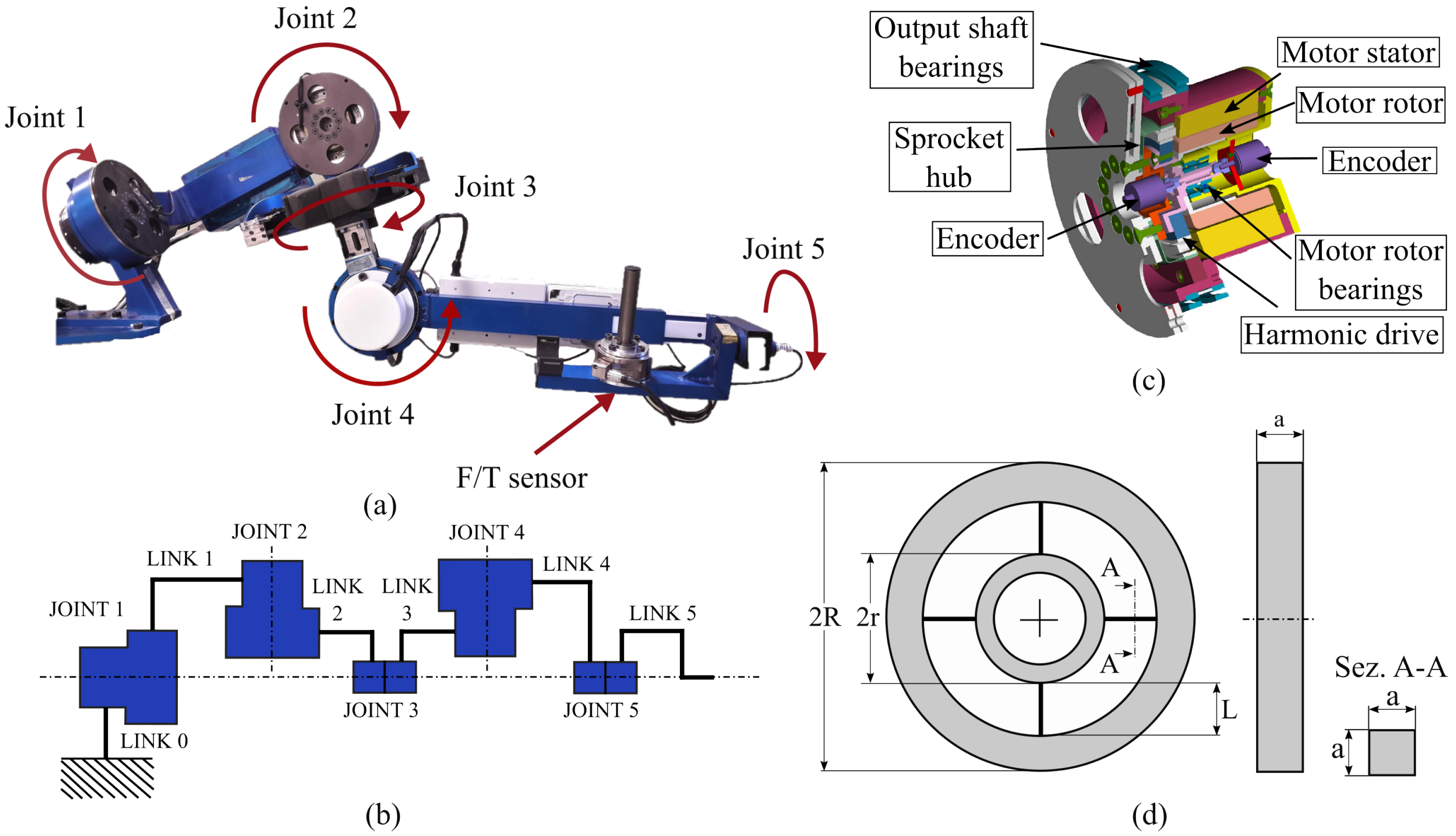
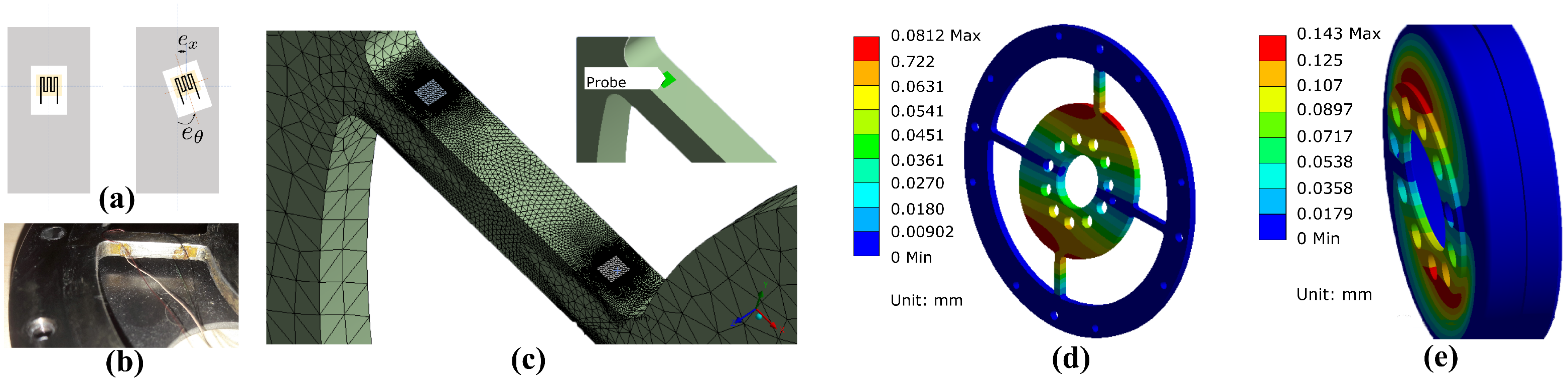
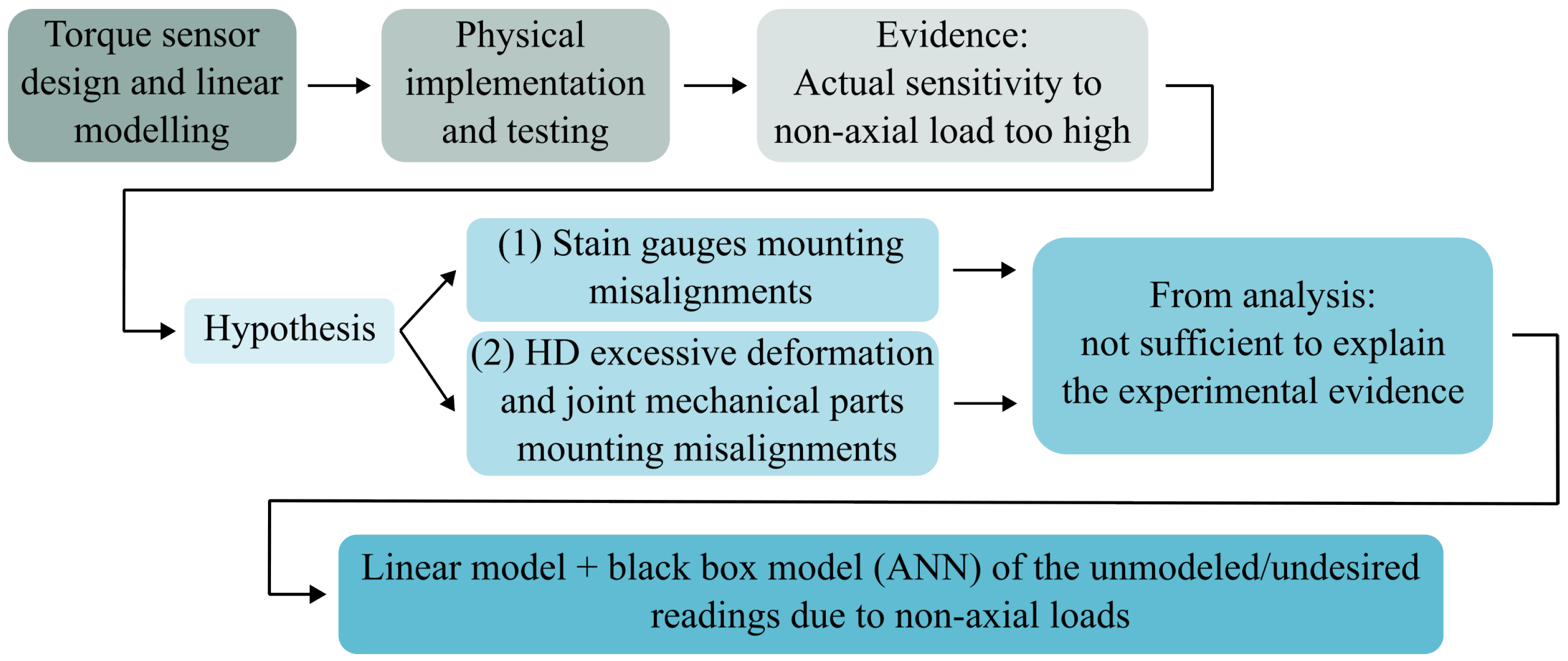
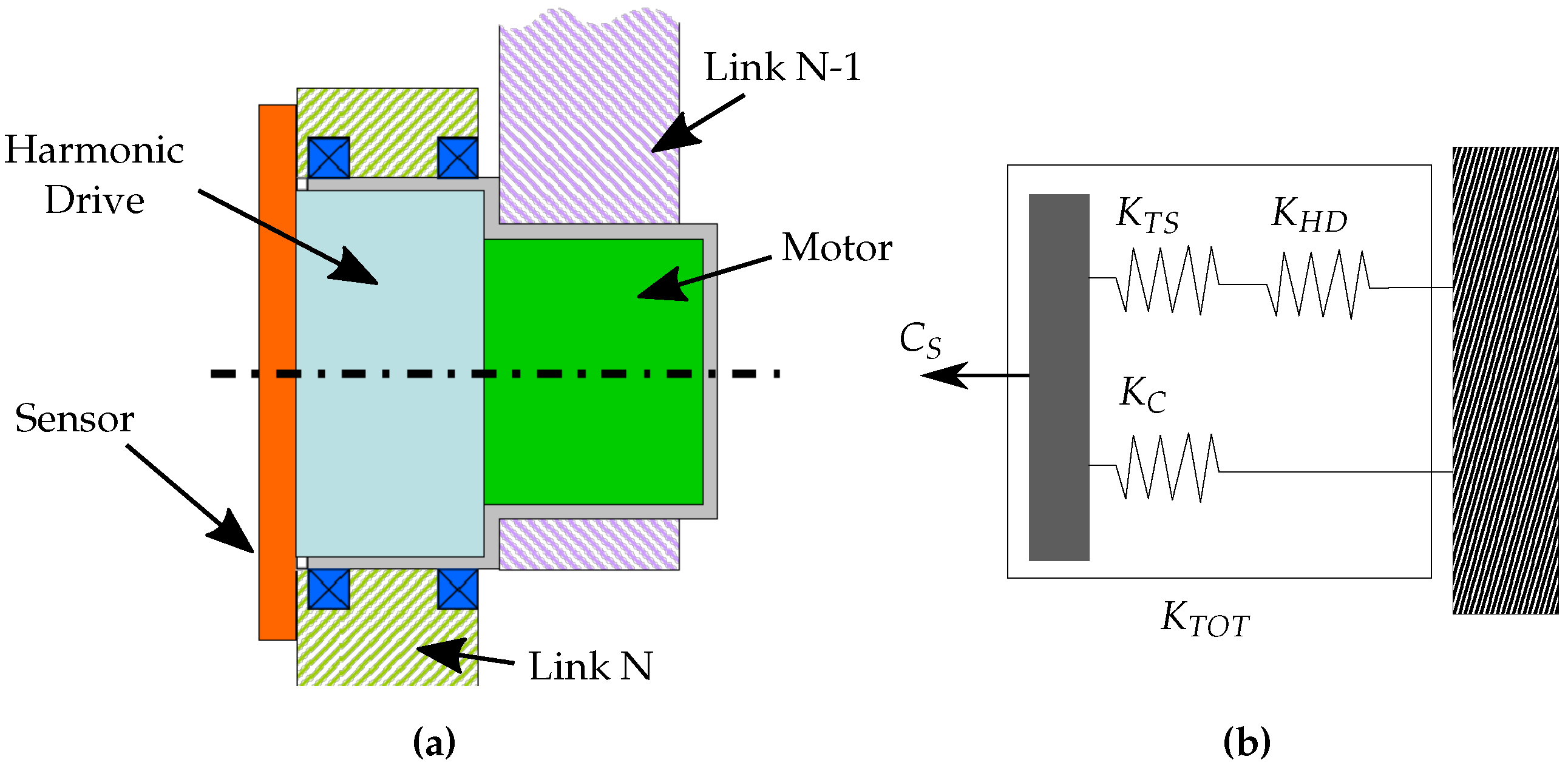
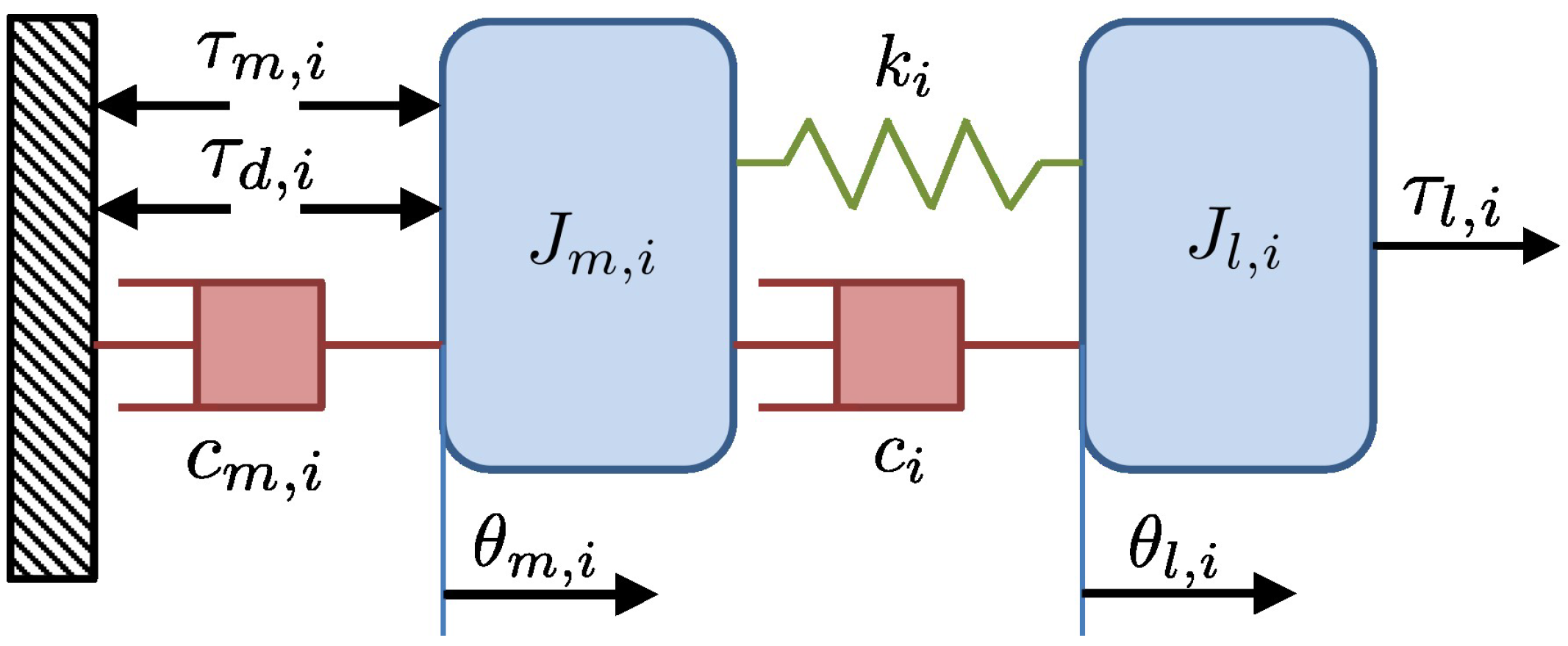
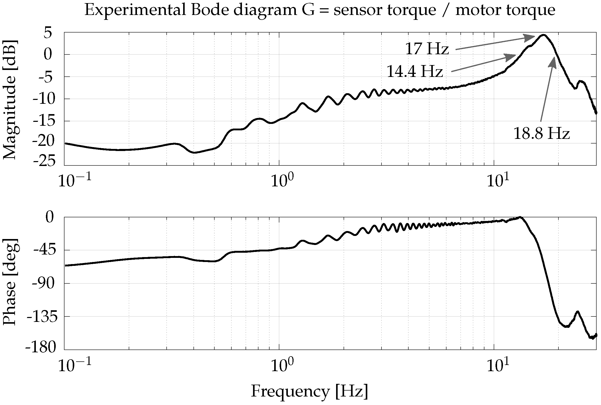
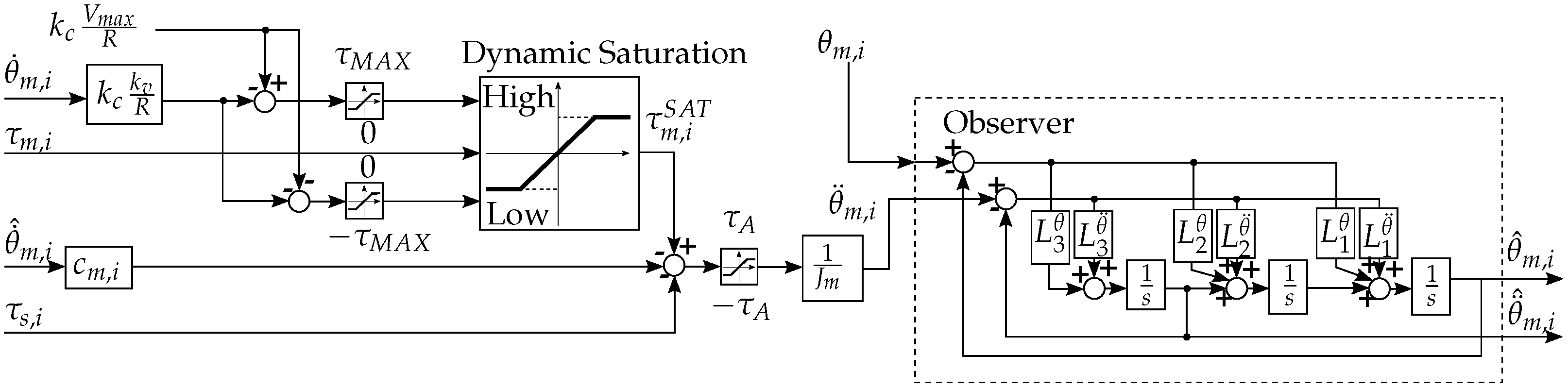
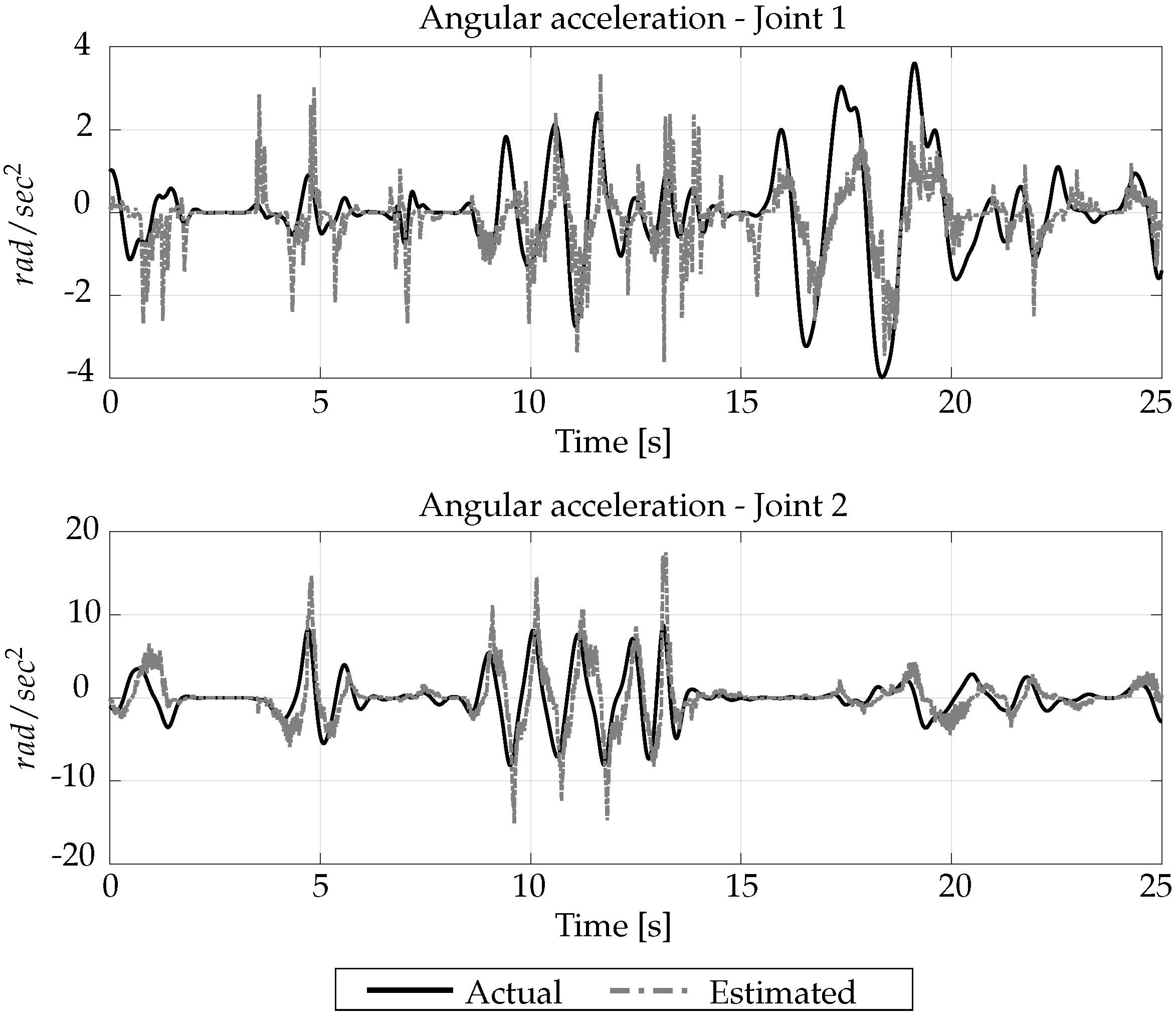
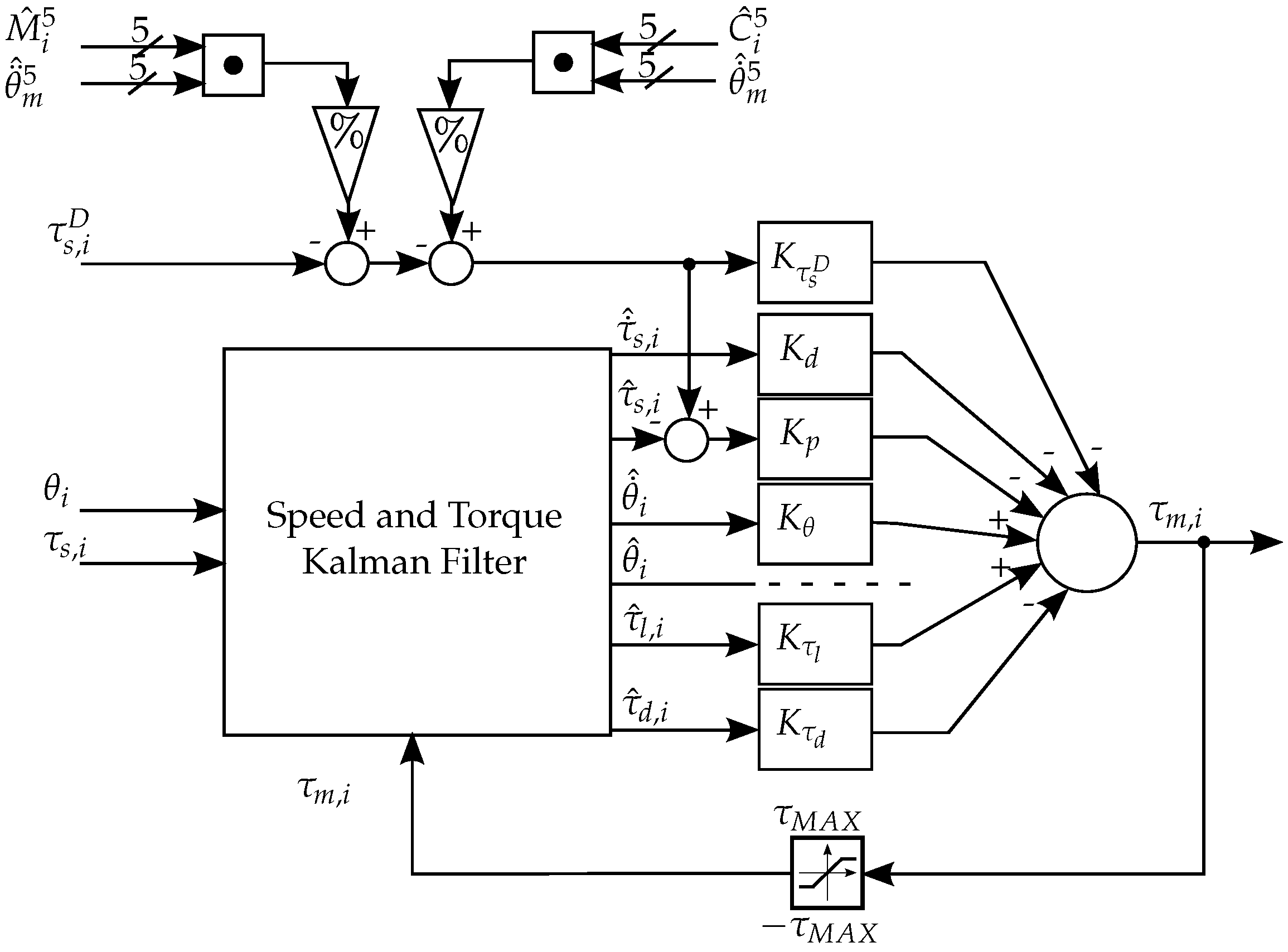
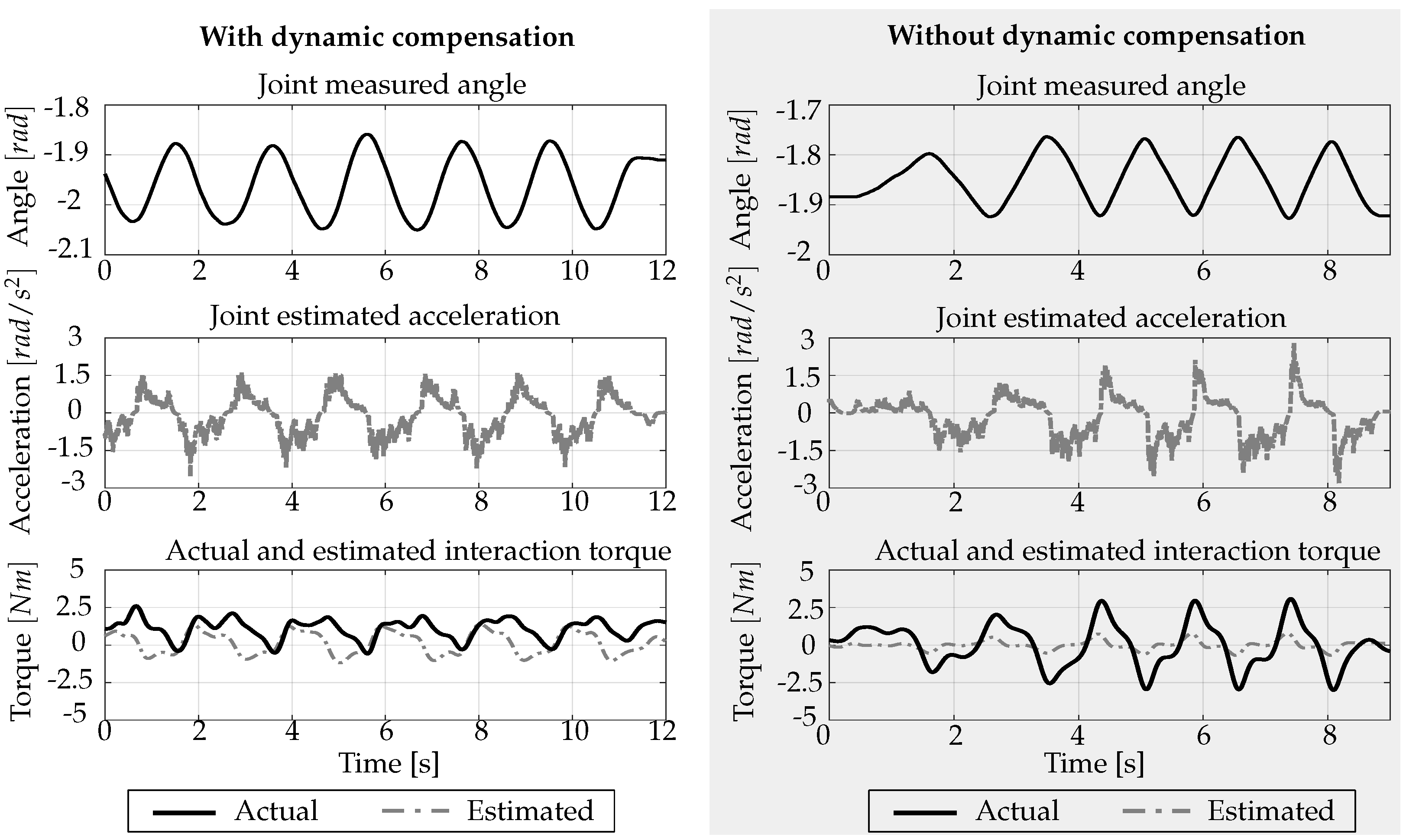
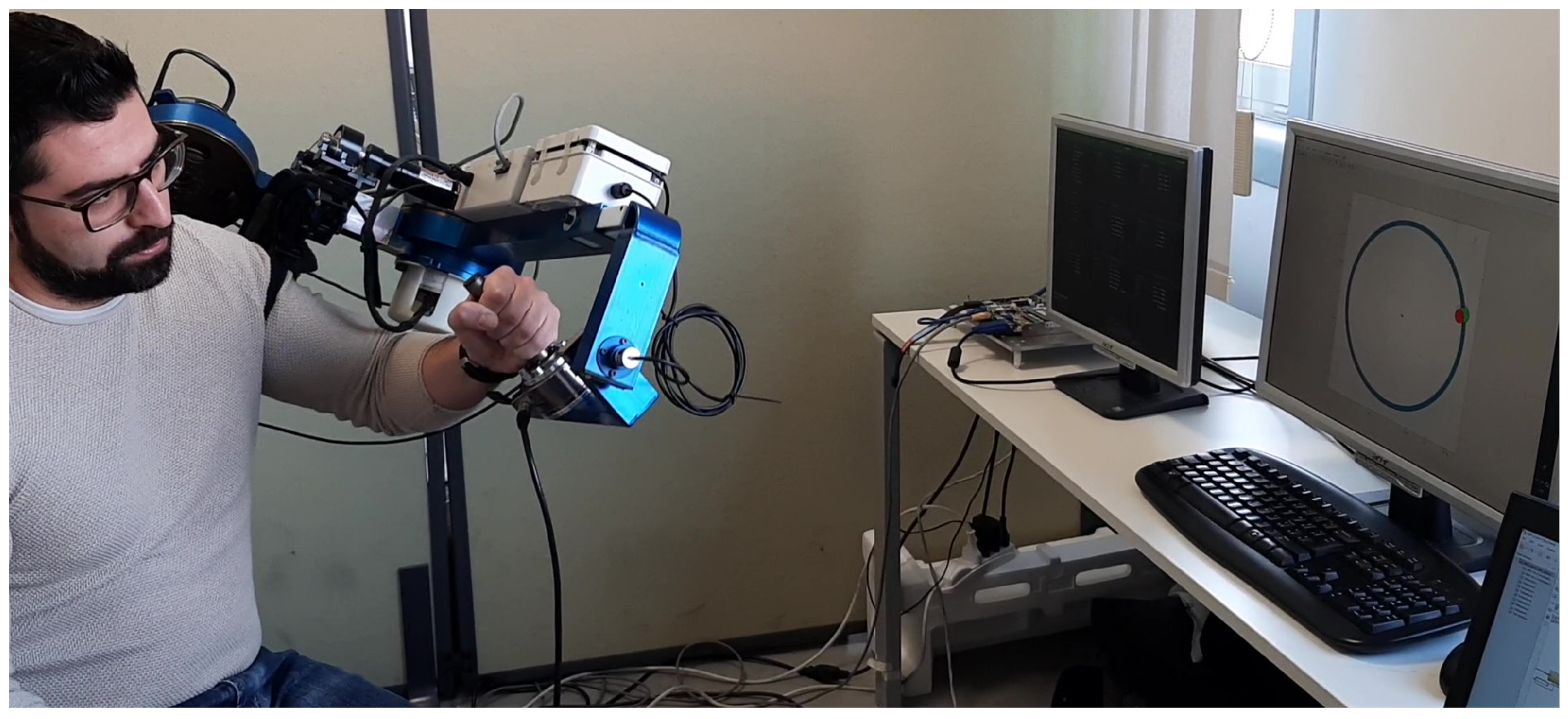
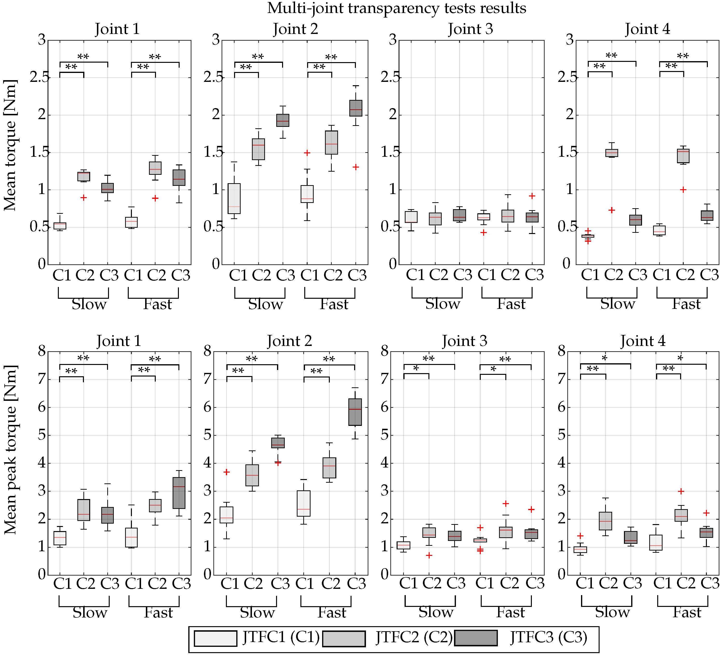
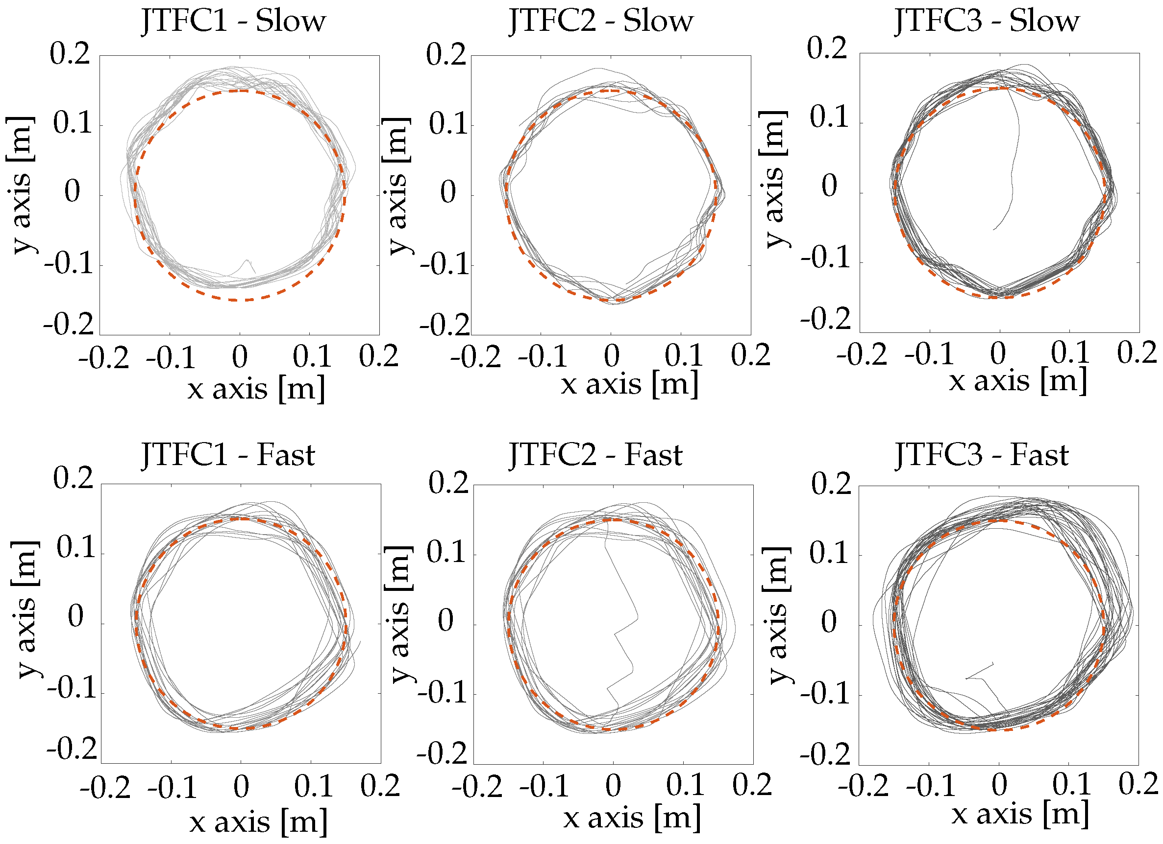
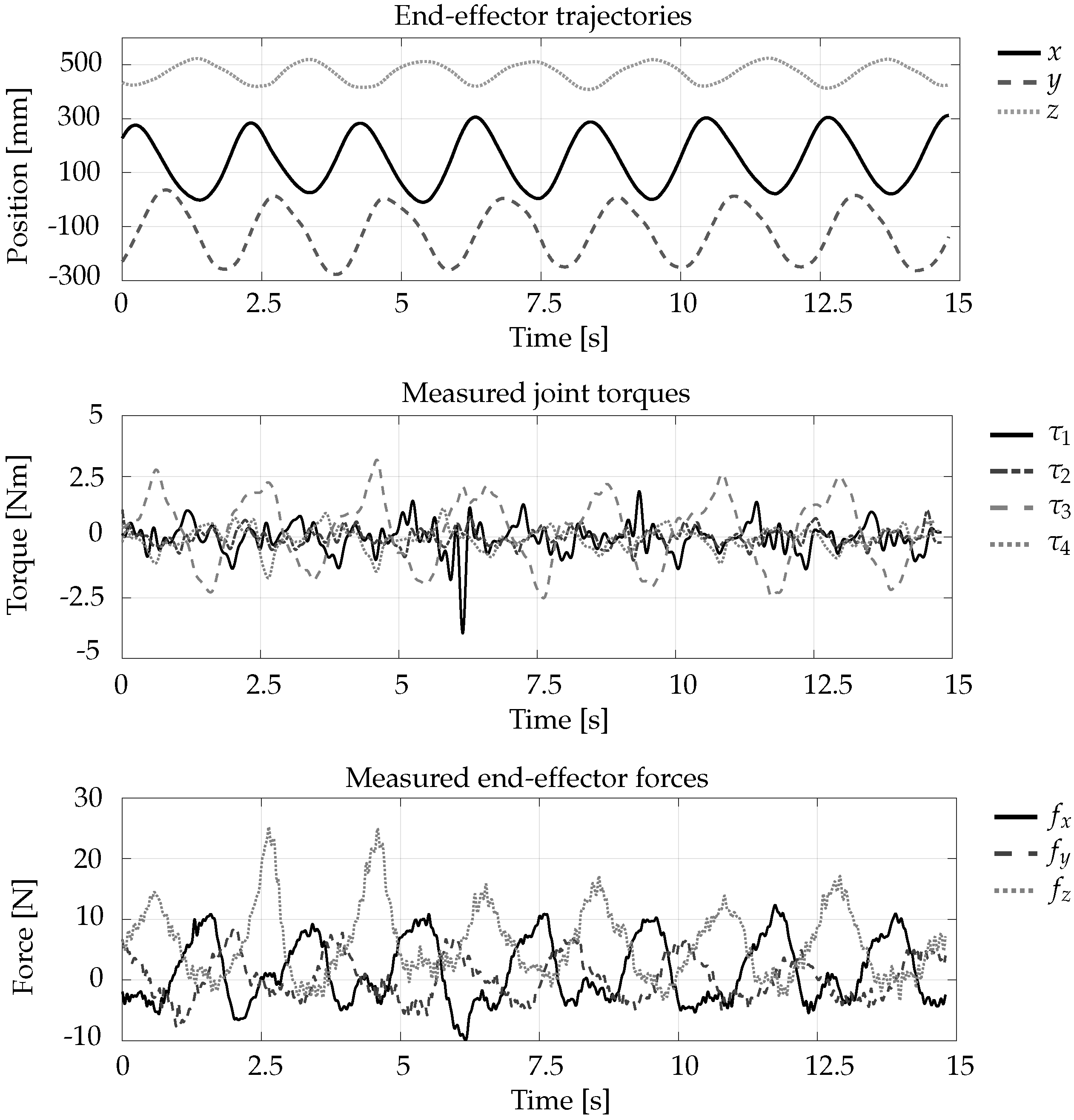
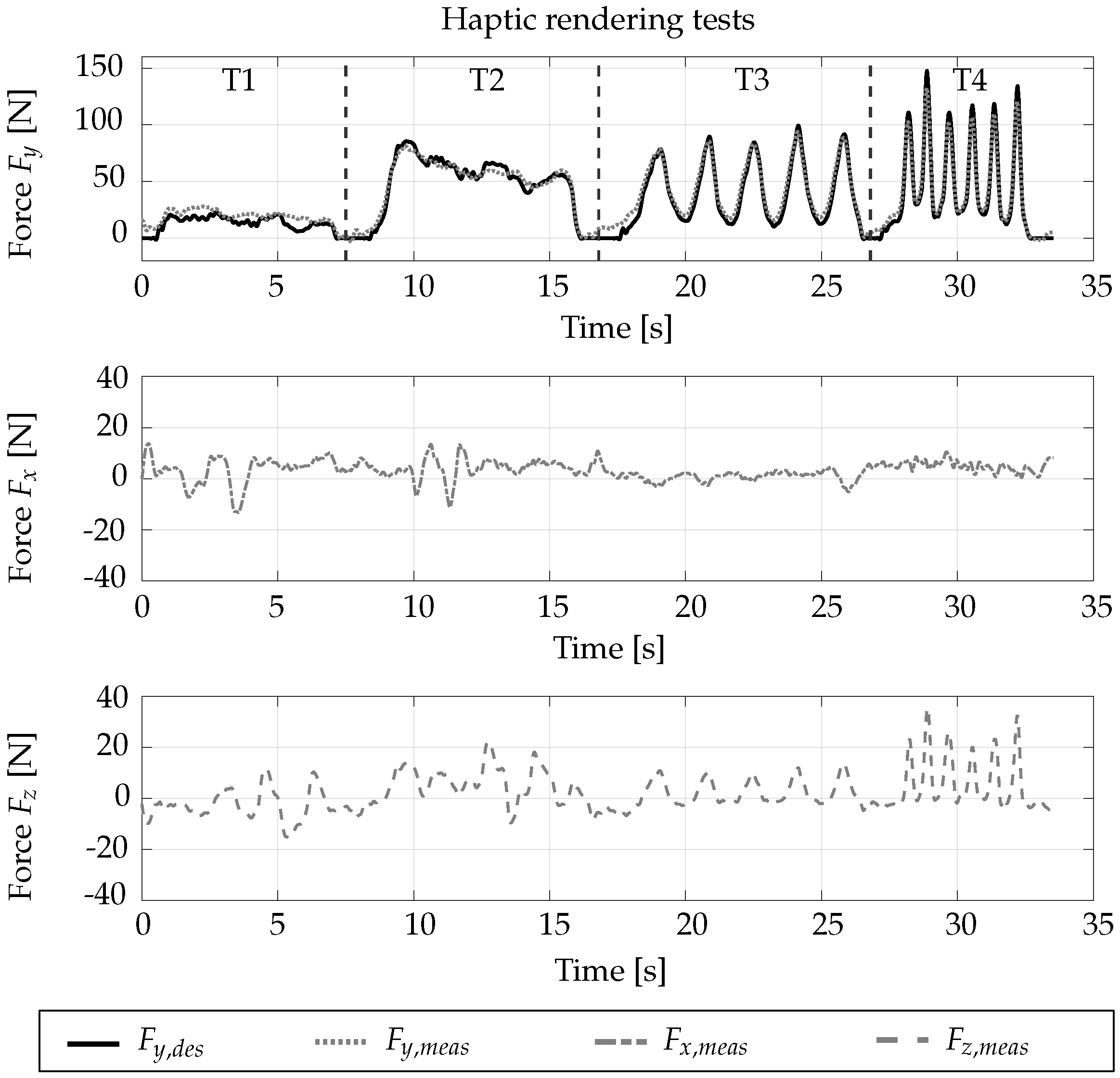
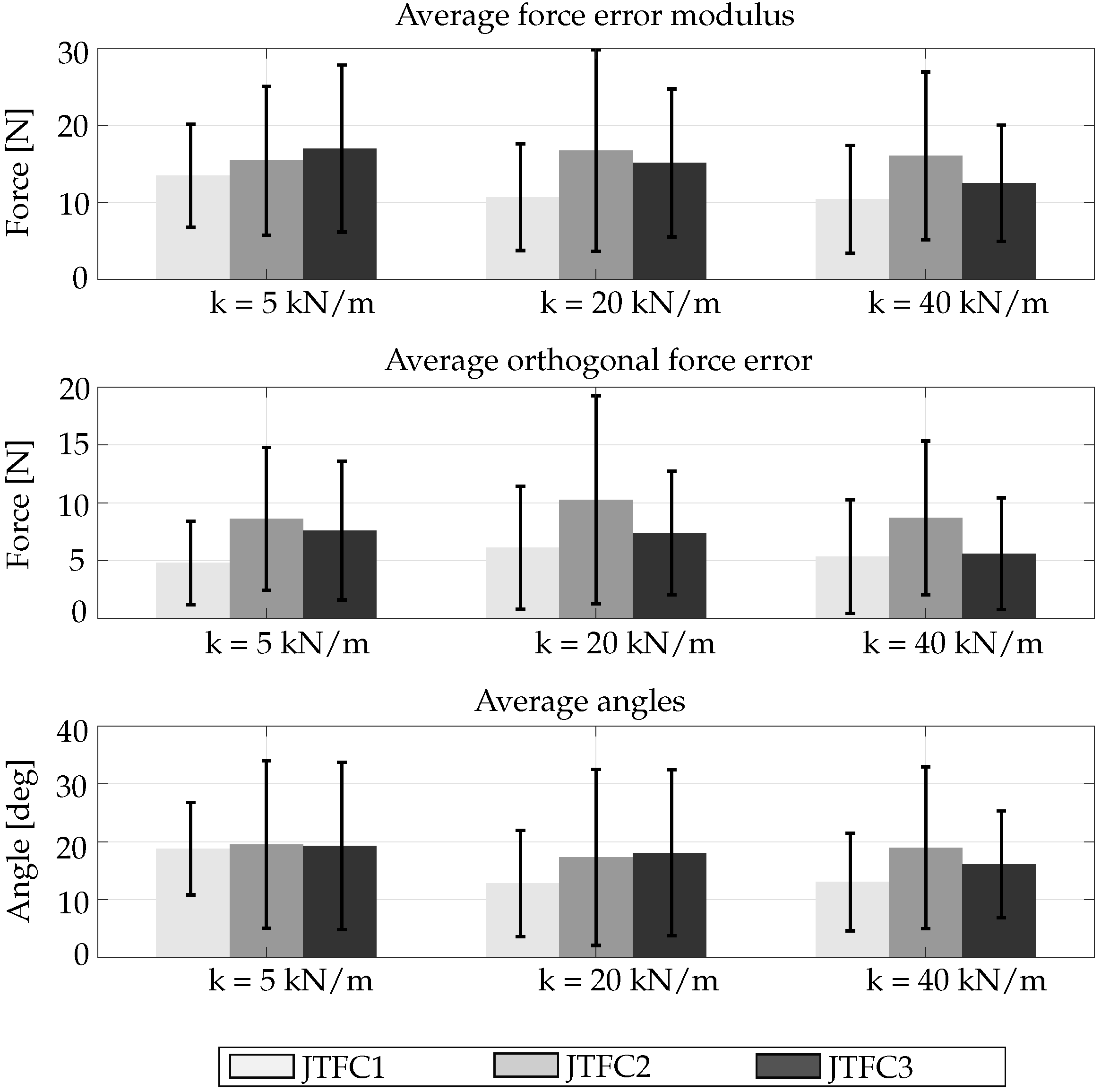
Table 1.
List of advantages and disadvantages of the SEA, VSA and active impedance by control solutions. This list is not exhaustive.
Table 1.
List of advantages and disadvantages of the SEA, VSA and active impedance by control solutions. This list is not exhaustive.
| pHRI Actuator Solution | Advantages | Disadvantages |
|---|---|---|
| SEA | Smaller requested motor peak power; safety | Fixed stiffness; torque estimation relies on the encoder readings and sensor accuracy |
| VSA | Versatility; smaller requested motor peak power; safety | Increased complexity; need for auxiliary motor, mechanics and control; more weight |
| Active impedance by control | Lightness; compactness; robustness | Time response and dynamic bandwidth is limited by the control system and actuators’ electrical properties |
Table 2.
Characteristic dimensions of the torque sensor.
| Dimension | R | r | L | a |
|---|---|---|---|---|
| Value (mm) | 78 | 38 | 24 | 4 |
Table 3.
Strain of the four strain gauges.
| Probe 1 | Probe 2 | Probe 3 | Probe 4 |
|---|---|---|---|
Table 4.
Sensor readings referring to non-axial moment sensitivity.
| Applied Torque (Nm) | Sensor Readings Per Angle (Nm) | |||
|---|---|---|---|---|
| 0° | 45° | 90° | 180° | |
| 32 | 1.6 | 2.4 | 2.2 | 2.3 |
| 64 | 2.9 | 4.8 | 4.4 | 4.4 |
| 96 | 4.5 | 7.5 | 6.9 | 6.9 |
Table 5.
Stiffness of the components.
| Component | Stiffness (kNm/rad) |
|---|---|
| 4.1 | |
| 0.4 | |
| 23.6 | |
| 24 |
Table 6.
The natural frequency of the joints.
| Joint | Avg. Link Inertia (kg/m2) | Natural Freq. (Hz) |
|---|---|---|
| 1 | 0.9639 | 19.3930 |
| 2 | 1.11 | 18.3501 |
| 4 | 0.1925 | 39.6797 |
Table 7.
Values of the parameters of each joint for the JTFC1, JTFC2 and JTFC3 controllers.
| JTFC1 | JTFC2 | |||||
| d | 3.2 | 6 | 2 | 4 | 7 | 2 |
| 15.89 | 0.82 | 0.33 | 34.39 | 13.89 | 12.01 | |
| 0.26 | 0.25 | 0.16 | 0.45 | 0.54 | 0.21 | |
| JTFC3 | ||||||
| d | 0.11 | 0.09 | 0.16 | |||
| 9.43 | 5.21 | 9.84 | ||||
| 0.005 | 0.0027 | 0.005 | ||||
Table 8.
Mean torque and mean peak torque for JTFC1.
| Speed | J1 | J2 | J3 | J4 | |
|---|---|---|---|---|---|
| Mean | Slow | 0.54 | 0.77 | 0.57 | 0.39 |
| torque (Nm) | Fast | 0.58 | 0.88 | 0.63 | 0.44 |
| Mean peak | Slow | 1.35 | 2.05 | 1.07 | 0.93 |
| torque (Nm) | Fast | 1.36 | 2.36 | 1.24 | 1.06 |
Table 9.
Smoothness index for the 3 controllers.
| Speed | JTFC1 | JTFC2 | JTFC3 |
|---|---|---|---|
| Slow | 80.87 | 47.10 | 47.80 |
| Fast | 107.46 | 85.48 | 119.08 |
Table 10.
The average forces involved in the T1 and T2 trials, the average force peaks and the average slope of the T3 and T4 trials.
Table 10.
The average forces involved in the T1 and T2 trials, the average force peaks and the average slope of the T3 and T4 trials.
| 5 kN/m | 20 kN/m | 40 kN/m | |
|---|---|---|---|
| 2 Ns/m | 7 Ns/m | 10 Ns/m | |
| Avg. force T1 (N) | 22.22 | 22.81 | 24.98 |
| Avg. force T2 (N) | 50.79 | 66.14 | 59.37 |
| Avg. peaks T3 (N) | 83.33 | 103.97 | 88.32 |
| Avg. slope T3 (N/s) | 127.28 | 159.25 | 120.39 |
| Avg. peaks T4 (N) | 112.33 | 136.97 | 126.20 |
| Avg. slope T4 (N/s) | 518.49 | 550.99 | 616.03 |
Disclaimer/Publisher’s Note: The statements, opinions and data contained in all publications are solely those of the individual author(s) and contributor(s) and not of MDPI and/or the editor(s). MDPI and/or the editor(s) disclaim responsibility for any injury to people or property resulting from any ideas, methods, instructions or products referred to in the content. |
© 2024 by the authors. Licensee MDPI, Basel, Switzerland. This article is an open access article distributed under the terms and conditions of the Creative Commons Attribution (CC BY) license (https://creativecommons.org/licenses/by/4.0/).
Share and Cite
MDPI and ACS Style
Chiaradia, D.; Rinaldi, G.; Solazzi, M.; Vertechy, R.; Frisoli, A. Design and Control of the Rehab-Exos, a Joint Torque-Controlled Upper Limb Exoskeleton. Robotics 2024, 13, 32. https://doi.org/10.3390/robotics13020032
AMA Style
Chiaradia D, Rinaldi G, Solazzi M, Vertechy R, Frisoli A. Design and Control of the Rehab-Exos, a Joint Torque-Controlled Upper Limb Exoskeleton. Robotics. 2024; 13(2):32. https://doi.org/10.3390/robotics13020032
Chicago/Turabian StyleChiaradia, Domenico, Gianluca Rinaldi, Massimiliano Solazzi, Rocco Vertechy, and Antonio Frisoli. 2024. "Design and Control of the Rehab-Exos, a Joint Torque-Controlled Upper Limb Exoskeleton" Robotics 13, no. 2: 32. https://doi.org/10.3390/robotics13020032
Note that from the first issue of 2016, this journal uses article numbers instead of page numbers. See further details here.