
A Passivity-Based Framework for Safe Physical Human–Robot Interaction


1
Electrical and Computer Engineering Department, University of Central Florida (UCF), Orlando, FL 32816, USA
2
ECE and NanoScience Technology Center, University of Central Florida (UCF), Orlando, FL 32816, USA
*
Author to whom correspondence should be addressed.
Robotics 2023, 12(4), 116; https://doi.org/10.3390/robotics12040116
Submission received: 21 July 2023
/
Revised: 6 August 2023
/
Accepted: 11 August 2023
/
Published: 14 August 2023
(This article belongs to the Section Humanoid and Human Robotics)
Abstract
:In this paper, the problem of making a safe compliant contact between a human and an assistive robot is considered. Users with disabilities have a need to utilize their assistive robots for physical human–robot interaction (PHRI) during certain activities of daily living (ADLs). Specifically, we propose a hybrid force/velocity/attitude control for a PHRI system based on measurements from a six-axis force/torque sensor mounted on the robot wrist. While automatically aligning the end-effector surface with the unknown environmental (human) surface, a desired commanded force is applied in the normal direction while following desired velocity commands in the tangential directions. A Lyapunov-based stability analysis is provided to prove both the convergence as well as passivity of the interaction to ensure both performance and safety. Simulation as well as experimental results verify the performance and robustness of the proposed hybrid controller in the presence of dynamic uncertainties as well as safe physical human–robot interactions for a kinematically redundant robotic manipulator.
1. Introduction
While assistive robotic devices such as Wheelchair-Mounted Robotic Arms (WMRAs) [1,2,3,4,5] and Companion Robots [6,7,8,9,10] traditionally help users with object retrieval [11,12] or pick-and-place tasks [13], they are quite capable of physical human–robot interaction (PHRI) with the user themselves. Users with disabilities have a need for assistance with activities of daily livings (ADLs) such hair-grooming, scratching, face-sponging, etc.; these ADLs require physical interaction with various surfaces on the human body. Under this need, the assistive robot’s end-effector (tool) has to be able to align with the unknown (human) surface, and also apply a desired force in the normal direction while following the surface based on desired velocity profiles that the user can command to the robot. During interaction, it is paramount to ensure that the assistive robot can establish safe and compliant contact with the human user.
Researchers have proposed various methods to achieve hybrid position/force control on a surface. In [14], the author used the exact CAD model for polishing position/force control. With the CAD/CAM model, they are able to track the desired trajectory, force, and contact direction. Since it requires an exact CAD model of the environment, this method will not work for the PHRI problem considered in this paper, which is likely to be implemented in unmodeled real-world environments. In [15], the authors designed and implemented a compliant arm to perform bed baths for patient hygiene. A bang-bang controller was utilized to maintain the z-axis force against the body between 1 and 3 N while a laser range finder was utilized to retrieve the skin surface point cloud of the skin followed by selection of wiping area by the operator. This method also requires obtaining the point cloud of the environment. The authors of [16] proposed a contact force model for wiping and shaving tasks. They captured the face point cloud and the force profile of healthy participants performing daily living tasks such as wiping and shaving. Then, they built a three-parameter trapezoidal force model of each stroke and the force dependency on the facial area. Besides assuming previous knowledge of the environment, there are other approaches for unknown environments. In [17], the author proposed two methods for exploring unknown surfaces with discontinuities by using only a force/torque sensor. They rotated the direction of the desired motion/force instead of rotating the end-effector to keep moving and inserting force on an unknown surface; however, this method cannot be used for certain PHRIs which need continuously variable alignment between the end-tool and human body, such as during shaving. In [18], the authors proposed a hybrid position/force sliding mode control for surface treatment such as polishing, grinding, finishing, and deburring—the end-effector can apply the desired pressure on the surface and also keep the end-effector orientation perpendicular to the surface; however, the orientation constraint is not considered for moving along a frictional environment. In [19], the authors proposed deformation-tracking impedance control for interacting with unknown surfaces by using an extended Kalman filter to estimate the parameters of the environment, thereby controlling the interaction force indirectly by tracking the desired deformation without force sensing. However, this method cannot estimate the interaction torque; therefore, during the alignment phase of the assembly task, their desired interaction torque is just determined experimentally. In [20], the authors proposed an inverse differential kinematics-based position/force control for cleaning an unknown surface. They utilized a force/torque sensor to provide feedback for the force control part. However, this velocity-control-based algorithm is not considered safe for human–robot interaction; furthermore, the evaluation of surface alignment is also missing.
In this paper, we propose a robust hybrid force/velocity/attitude controller which guarantees passivity of a robot manipulator with respect to unknown environments. By using measurements of robot states as well as interaction forces/torques at the end-effector, we are able to reshape the end-effector impedance (namely inertia, damping, and stiffness) to desired values needed for a safe and compliant interaction. Sliding mode control is utilized to compensate for exogenous disturbances, model uncertainty, and friction effects which can otherwise degrade the performance of the impedance controller. Within the sliding mode controller, we are able to achieve the desired system dynamics with a general assistive robot, which has a lower cost and less precision than industry collaboration robots. The resulting controller is able to align the end-effector with the unknown environmental surface while simultaneously tracking desired force and velocity profiles, respectively, in the normal and tangential directions. This work is novel in terms of the guarantees of 6-DOF exponential stability and passivity of our hybrid controller while interacting with an unknown environment.
The remainder of this paper is organized as follows. Section 2 and Section 3 deal, respectively, with the problem statement and the modeling. In Section 4, we present the controller design, stability analysis, proof of passivity, and simulation results for a frictionless environment. In Section 5, we present the corresponding control design and stability analysis for a real environment with friction. Experimental results with a kinematically redundant collaborative robot are presented in Section 6 (see [21] for visual demonstrations of the simulations and experiments). Section 7 concludes the paper.
2. Problem Statement
The research objective is to align the robot end-effector with the unknown environment and apply a desired force in the normal direction while following a commanded velocity profile along the tangential directions. In order to guarantee safe human–robot interaction, another research objective is to ensure that the robot acts as a passive system while transmitting user intent to and during interaction with the environment. To design and implement our robust impedance control framework, we assume knowledge of the joint position/velocity measurements as well as the interaction force at the end-effector using a wrist-mounted six-axis force/torque sensor. We assume uncertainty in the robot dynamics and no prior knowledge of the location/orientation of the environmental surface with respect to the robot coordinate system. While we assume that the surface presents damping and stiffness in the normal direction and pure damping along the surface, we assume no prior knowledge of the parameters; being model-free in this sense allows the controller the ability to interact with a variety of unknown environments.
3. Modeling
3.1. Manipulator Model
The dynamics of an n-degree-of-freedom robot are given by
where is the symmetric positive-definite inertia matrix, is the matrix of Coriolis and centrifugal torques, is the vector of gravitational torques, denote, respectively, the joint angle, joint velocity, and joint acceleration vectors, is the control input vector of joint torques, is the external torque registered at the robot joints, is the interaction force measured with the force/torque sensor mounted on the wrist, is the Jacobian matrix, while denotes joint friction. The joint velocity and acceleration for a redundant robot (i.e., ) can be written as follows:
where denote end-effector velocity and acceleration vectors, respectively, and are the end-effector translation and angular velocity expressed in the base frame, denotes the right pseudoinverse of the Jacobian matrix, while is an arbitrary vector utilized to accomplish secondary objectives such as joint limit, collision avoidance, etc. For ease of presentation, we choose for the remainder of the paper. After replacing the joint acceleration and velocity with (2) and (3), we can obtain the task space robot dynamics as follows:
To accomplish our velocity tracking objective, we define error in the end-effector frame as follows:
where denotes the desired translational velocity in the end-effector frame, and are, respectively, the end-effector translation and angular velocity expressed in the end-effector frame, while denotes the rotation matrix between the robot base frame and the end-effector frame. By utilizing the velocity tracking error expressed in the end-effector frame, can be related to the end-effector velocity variables in the base frame as follows
By rearranging (5) and taking its time derivative, one can obtain the following expressions for and :
By substituting (6) and (7) in (4), we can obtain the open-loop error dynamics as follows:
where We denote the best-guess estimates of and U, respectively, as , and , while , and denote the corresponding uncertainties. Based on these definitions, we can rewrite the open-loop error dynamics as follows:
where
is a lumped model uncertainty term. Before proceeding further, we are motivated by the structure of the robot dynamics and the ensuing control development and stability analysis to assume the existence of the following properties:
- Property 1
- All kinematic singularities are always avoided and the pseudoinverse of the manipulator Jacobian, denoted by , is assumed to always exist.
- Property 2
- Property 3
- The inverse of the inertia matrix is assumed to be bounded by a known positive constant as , where denotes a known positive bounding constant [23].
- Property 4
- Based on Properties 2 and 3, the lumped model uncertainty term D defined above in (10) can be upper bounded by a function of the joint velocity as follows:where , and denote known positive bounding constants.
3.2. Environment Model
We model the environment as a spring-damper which provides the environmental force in the object (environment) frame as follows:
where are diagonal matrices of environment stiffness and damping, respectively, denotes the standard basis vector in the z-direction, while is the z-axis neutral position of the environment in the object frame, and is the current z-axis position of the end-effector expressed in the object frame. Here, is the velocity of the end-effector with respect to the object expressed in the object frame, is the end-effector translational velocity as defined earlier, while is the unknown rotation matrix between the object frame and end-effector frame. In the end-effector frame, the environmentally exerted torque on the end-effector can be defined as follows:
where is the unknown position vector from the center of the sensor to the contact point while is the environmental force expressed in the end-effector frame. The model of the interaction between the end-effector and the environment is shown in Figure 1.
We also model the end-tool for the manipulator as a rigid partial sphere as specified in Figure 2. In the figure, denotes the center of the robot wrist where the six-axis force/torque sensor is mounted, denotes the center of the sphere, is the position vector from the sphere center of the end-tool to the contact point, while is the position vector from the sphere center to the robot wrist center and is parallel with the end-effector z-axis denoted by .
4. Control Design and Stability Analysis: Non-Dissipative Environment
4.1. Control Design
The proposed control design has an inner and an outer loop. While the inner loop is a robust controller to compensate for the system uncertainties and linearize the robot dynamics, the outer loop reshapes the linearized dynamics to the desired dynamics. In what follows, we discuss the design of control strategies within the two loops that guarantee robust stability, convergence, as well as passivity. For lucidity of presentation, we first demonstrate PHRI stability and passivity when interacting with a non-dissipative (frictionless) environmental surface.
4.1.1. Design of the Inner Loop
Based on the structure of the open-loop error dynamics in (8) and our desire to obtain an impedance controller, we first design a computed torque inner-loop controller to linearize the dynamics as follows:
By substituting (14) into (9), we can obtain
In (14), is an auxiliary control term that is designed to compensate for the disturbance using a sliding mode controller as follows:
where is a yet-to-be-designed auxiliary control term related to the desired dynamics. Motivated by the bound in (11) and in a manner similar to [22], we design the gain, Q, for the function (the standard signum) as follows:
where is a positive design constant, , and have been introduced earlier in (11), while S denotes a sliding surface which is defined as follows:
such that
Then, we have the following result for the inner loop:
Lemma 1.
4.1.2. Design of the Desired Dynamics
To meet our velocity and force control objectives while projecting desired impedance characteristics on the environment, we propose the following desired dynamics in the translational axes:
where denote desired mass, damping, and stiffness matrices (note all non-zero matrix elements are positive design constants), while denotes the force error with denoting the desired force in the z-direction. In order to achieve the desired dynamics of (23), the auxiliary control term can now be designed as follows:
For the angular axis, we design a quaternion-based controller to align the end-effector with the unknown environment. The rotation between the end-effector z-axis and the environmental normal can be represented by a unit quaternion where , and and n are the angle and the rotation axis between and . The quaternion can be extracted from the torque and force feedback as follows. Based on the definition of the environment torque from (13) and the geometry of the end-tool in Figure 2, we can rewrite the environmental interaction torque as follows:
Since the environmental surface is assumed frictionless and based on the geometry of the end-tool shown in Figure 2, it is evident that and , where the notation ‖ denotes parallel vectors. Then, we can simplify the relationship expressed in (25) as
Now, it is possible to calculate the rotation axis n as follows:
Since the rotation direction is already contained in the vector n, the range of the angle between and is . From (26), we can calculate the angle between and as
The dynamics of the unit quaternion are as follows:
To reshape the angular dynamics in a desired mass/damper form, we begin by designing the desired rotational dynamics as follows:
where is the desired rotational inertia, while and u are, respectively, a damping matrix and an auxiliary control input which are yet to be designed. By taking the time derivative of a filtered tracking error ( is diagonal positive-definite) and premultiplying by , we obtain
which, by substitution of (29) and (30), can be rewritten as
Motivated by the ensuing stability analysis, we design u as follows:
such that
where is a positive-definite matrix. Now, it is possible to rewrite the desired rotational dynamics in the following compact form:
where is a positive time-varying damping matrix, while
is an auxiliary torque vector which is well defined everywhere on the domain of the problem. Finally, we can design the auxiliary control term defined in (16) as follows:
The overall proposed controller is shown in Figure 3.
4.2. Stability Analysis
Before presenting the main results, we state the following lemmas which will be invoked later.
Lemma 2.
The desired dynamics of the angular axis in (35) are locally exponentially stable at the equilibrium point () in the sense that , when , which implies that when the robot is interacting with a frictionless environment.
Proof.
Inspired by [25], we define a non-negative function as follows
which can be upperbounded as follows
by utilizing the fact that . After taking the derivative of (37) along (34) and (29) and canceling common terms, we can obtain
It is easy to see from (37) and (39) that From this and previous definitions, it follows that . Then, one can utilize Barbalat’s Lemma [23] to prove that which implies that . Since can be lowerbounded as follows:
it is easy to see from (38) and (40) that , where Thus we can conclude that the equilibrium point () is exponentially stable in the sense specified in the statement of the Lemma. □
Lemma 3.
The desired dynamics of the translational axes in (23) are globally exponentially stable (GES) at the equilibrium point () when the robot is interacting with a frictionless environment. Furthermore, , , , while
Proof.
We begin our analysis in the x- and y-axes. The desired dynamics in the x- and y-axes are as follows:
where the notation is obvious from context given the previous definitions. Since (41) is a second-order LTI system with eigenvalues in the strict LHP, the equilibrium point () is GES. As for the z-axis, the desired dynamics of (23) in that direction can be written as follows:
Since we are assuming no environmental friction, we can simplify (12) as
the time derivative of which can be written as
To facilitate the analysis, we take the time derivative of (42) and obtain the dynamics as
which is a second-order linear system with perturbation defined in (A1) in Appendix A. By utilizing (A2)–(A4), we can upperbound as follows:
where is a state vector. Given this definition, we rewrite (45) as follows:
where denotes the standard basis vector in the x-direction while A is a Hurwitz matrix defined in Appendix A. We also define a positive- definite function whose derivative along (47) is
where P and Q are defined in the Appendix A. After utilizing the growth bound of (46), we can upperbound (48) as follows
which implies exponential stability of in the following sense
where and denotes the unit step function. Therefore, is exponentially stable in the sense that where is a sufficiently large constant of analysis. Following the same process as in the proof for Lemma 2, it can be shown that , which implies, according to (42), that and that . Since it is evident that . □
Remark 1.
From Lemma 1, it can be seen that the closed-loop dynamics converge to the desired dynamics in (23) and (35) such that the desired impedance characteristics can be projected on the frictionless environment. Based on Lemma 2, the quaternion q (which represents the tool–environment misalignment) converges to zero, which implies that the robot end-effector aligns with the frictionless environment. Furthermore, according to Lemma 3, the end-effector can reproduce the commanded end-effector velocities on the environmental tangential plane while applying the desired amount of force in a direction normal to the environment.
From the above Lemmas, we can also have the main passivity result for the proposed controller in the following theorem:
Theorem 1.
The proposed control law can ensure the work performed by the robot on the frictionless environment (human) is bounded in the sense that where is the force/torque applied by the robot on the environment.
Proof.
We split the work performed by the robot into two phases: (Part a) Work performed before reaching the desired dynamics: Since the sliding mode control has finite-time convergence, it will drive the system dynamics to the desired dynamics in finite time . So, the work performed by the robot from to is as follows:
Based on the stability analysis of the sliding mode controller, we know that , . During ,
Therefore, we can write
Given the definition of (24), we can rewrite (51) as follows:
which is nothing but a perturbed version of the desired translational dynamics driven by the additional input , which remains bounded between and is zero thereafter. Since we know from previous analysis that the solution for the desired dynamics of (23) stays bounded, the solution for the perturbed version driven by a bounded input over a finite time period will also stay bounded. A similar argument can be made for the angular velocity desired dynamics. Thus,
where is a positive constant of analysis. (Part b) After reaching the desired dynamics: The work performed by the robot on the environment is denoted by , and can be bounded as follows:
since as previously shown. Since we can bound
given that and where . Since and , it is easy to see that . Since as previously shown, it is clear to see that . Therefore, we can conclude that the total work performed by the robot end-effector during Parts a and b is , which proves passivity. □
4.3. Simulation Results
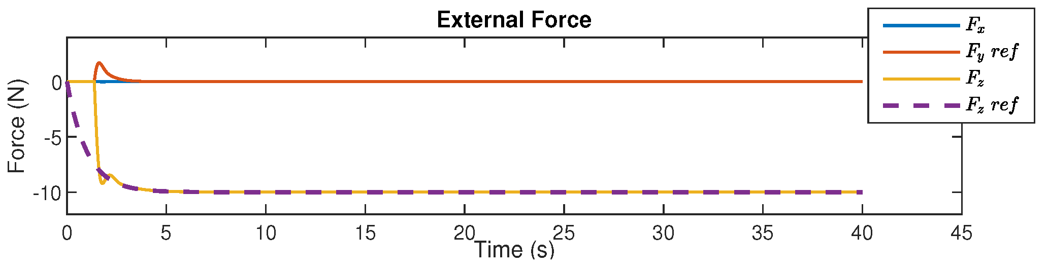
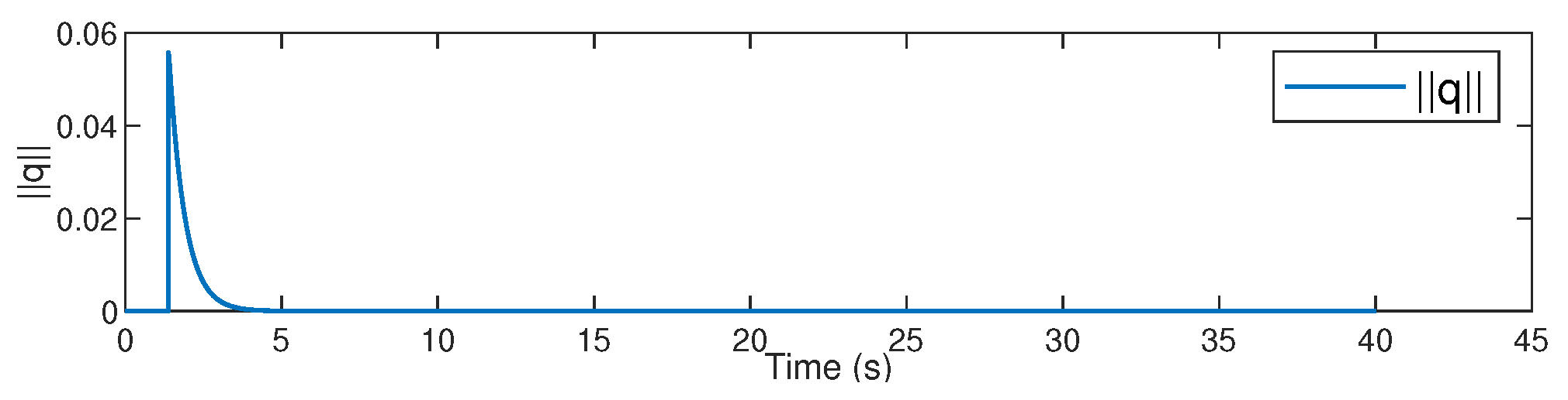
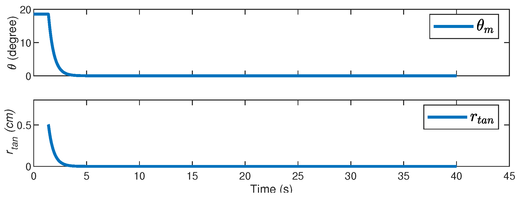
During the simulation, we choose 0–5 s as the initial alignment phase during which the commanded velocities in the x- and y-directions are both chosen to be 0 cm/s. Between 5–20 s and 20–35 s, we, respectively, command the desired velocity to be ±1.5 cm/s along the end-effector y-direction. Finally, between 35 and 40 s, we command 0 cm/s velocity in the tangential direction of the end-effector. From Figure 4, Figure 5, Figure 6, Figure 7 and Figure 8, we can see that the proposed controller can regulate the force error in end-effector z-direction to zero after the initial alignment process. The end-effector velocity along the tangential directions also tracks the desired velocity with nearly zero tracking error. As for the alignment, the norm of the quaternion and the misalignment angle decrease to 0. To evaluate the alignment, we define the so-called equivalent lever , which represents the length of projection of the lever arm in the end-effector x-y plane. When the end-effector is aligned with the environment, it is clear to see from Figure 8 that also converges to zero.
5. Control Design and Stability Analysis for Dissipative Environment
5.1. Control Design
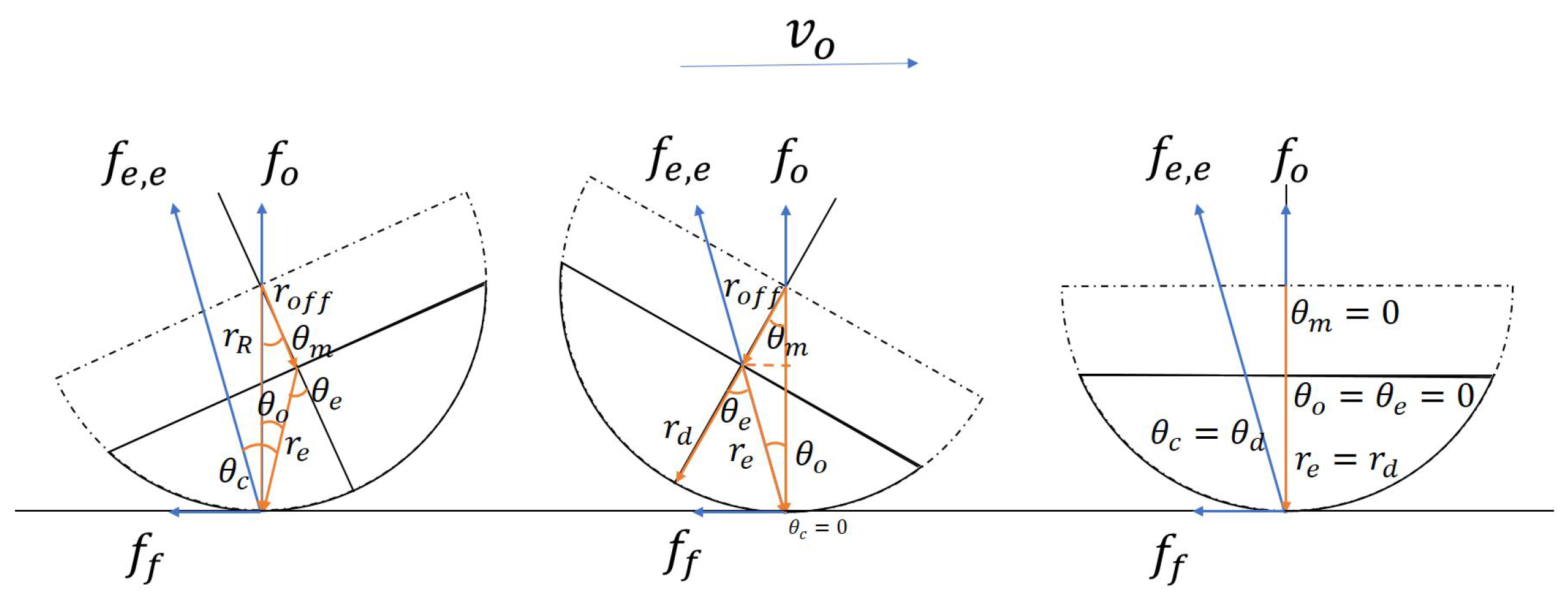
In the previous section, it is seen that the proposed controller is stable and passive during interaction with a frictionless environment. In this section, we will introduce the controller for a dissipative (frictional) environment, which is a better model for the real world. For the case with friction, we can design the sliding mode control and torque input as similarly carried out in Section 4.1, but if friction is not compensated for, even though the equilibrium for the angular axis remains the same (), the quaternion now represents the rotation between and ; therefore, the equilibrium represents . Since is the resultant of the friction force and the normal force from the object, the angle between the environment normal and is as for the geometry of the problem, there exists a non-zero misalignment angle between the end-effector and the environment normal which is related to the surface friction and the environment normal force. The orientation between the end-effector and environment can be seen in Figure 9.
To compensate for the misalignment due to friction, we design a desired torque and extract the desired quaternion , which represents the rotation between the desired lever arm and the environment force . Similar to the case without friction in Section 4.1.2, we can define and as follows:
where is the angle between and , while , where is the angle between and . Then, we define the quaternion error based on and
The quaternion dynamics are as follows:
With a process similar to that in Section 4.1.2, the desired dynamics of the rotation axis are designed as follows:
where
such that the dynamics of can be written as
Finally, we design the auxiliary control term as follows:
5.2. Stability Analysis
Lemma 4.
The desired dynamics of the angular axis in (59) is locally exponentially stable at the equilibrium point () when the robot is interacting with a frictional environment, in the sense that , for and a positive constant γ. Furthermore, the states of the angular axis
Proof.
For the environment with friction, our sliding mode control remains the same, but the desired dynamics in the angular axis are different. Based on the desired dynamics in (59) and the dynamics of quaternion error in (58), we can define a positive function similar to (37) as follows
where . After taking the time derivative of (62) along (58) and (60) and simplifying, we can obtain
With a process akin to that followed in the proof of Lemma 2 in Section 4.2, it is easy to see that the angular axis is exponentially stable at the equilibrium point () such that we can have and , which clearly implies that □
Lemma 5.
The desired dynamics of the translational axis in (23) are globally exponentially stable at the equilibrium point () when the robot is interacting with a frictional environment. Furthermore, , while
Proof.
The analysis for the x- and y-axes remains the same as in Section 4.2 but the model of the environmental force has the damping term due to non-zero as shown in (12). The time derivative of the the desired dynamics of (23) in the z-axis can be written as follows:
Given that can be written as
the second-order dynamics can of (63) can be compactly written after algebraic manipulations as follows:
where has been previously defined while is an additional term defined and bounded, respectively, in (A7) and (A8). It is now clear to see from (46) and (A8) that can be norm-bounded as follows:
where are positive constants. It is now possible to follow the analysis as pursued in Section 4.2 for the non-dissipative case to obtain exponential stability in the sense that , where and are positive constants of analysis. Since , it can be seen from (42) and (12) that , from which it is clear that since as shown in the Appendix A. This implies from (12) and (13) that . It can now be seen from (23) that □
Remark 2.
To summarize the analysis for the dissipative case, Lemma 1 shows that we can project the desired impedance on the frictional environment, which is then followed up by Lemmas 4 and 5, which show that the robot end-effector aligns with the environment and tracks the end-effector velocity along the environmental tangential axes while also applying the desired amount of force in the environmental normal direction.
Given the above Lemmas, the passivity result for the proposed controller can be stated in the following theorem:
Theorem 2.
The proposed control law can ensure the work performed by the robot over and above the dissipation expected from relative motion at the desired surface velocity between the end-effector and the frictional environment(human) is limited in the sense that where is the essential power expended.
Proof.
As similarly carried out in the proof of Theorem 1, we split the work performed by the robot into two phases: (Part a) Work performed before reaching the desired dynamics: Proof is identical to that for the frictionless environment shown earlier. (Part b) After reaching the desired dynamics: The work performed by the robot on the frictional environment is denoted by , and can be bounded as follows:
since as previously shown. After some algebraic manipulations as shown in the Appendix A, we can bound the first time in the above inequality as follows
Since , we can clearly see from (65) and (67) that . Putting together the results from Part a and Part b proves the passivity result as stated in the statement of the theorem. □
5.3. Simulation Results
In order to closely mirror experimental reality, we add joint friction, measurement noise, imperfect gravity compensation, and imperfect robot inertial matrix to the simulation studies. The joint friction model utilized is as follows
where are the Coulomb, static, and viscous friction coefficients, while is the Stribeck parameter. We also add measurement noise which follows a normal distribution with . We assume there is imperfect gravity compensation in the simulation. As for the imperfect robot inertial matrix, we assume there is a constant error in the inertial matrix for the last three joints. We assume a planar surface for the simulation. We also replace the function in the sliding mode control with a continues function to mitigate the chattering phenomenon. The parameters utilized for each joint are listed in Table 1.
During implementation, we treat and defined in (55) and (56) as immeasurable since is impractical to assume that the lever arm (as shown in Figure 2) is measurable. Instead, we replace the unknown value of with a known upperbound and redefine and as follows:
where and have been previously defined, while , , , . Here, is a constant, while is a function of . While the proof using the redefined quaternions is beyond the scope of this manuscript, it can be easily shown (see Appendix A) that the exponential convergence of to implies the exponential convergence of to .
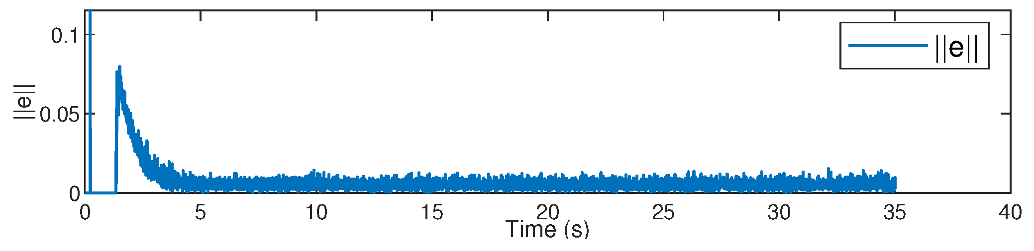
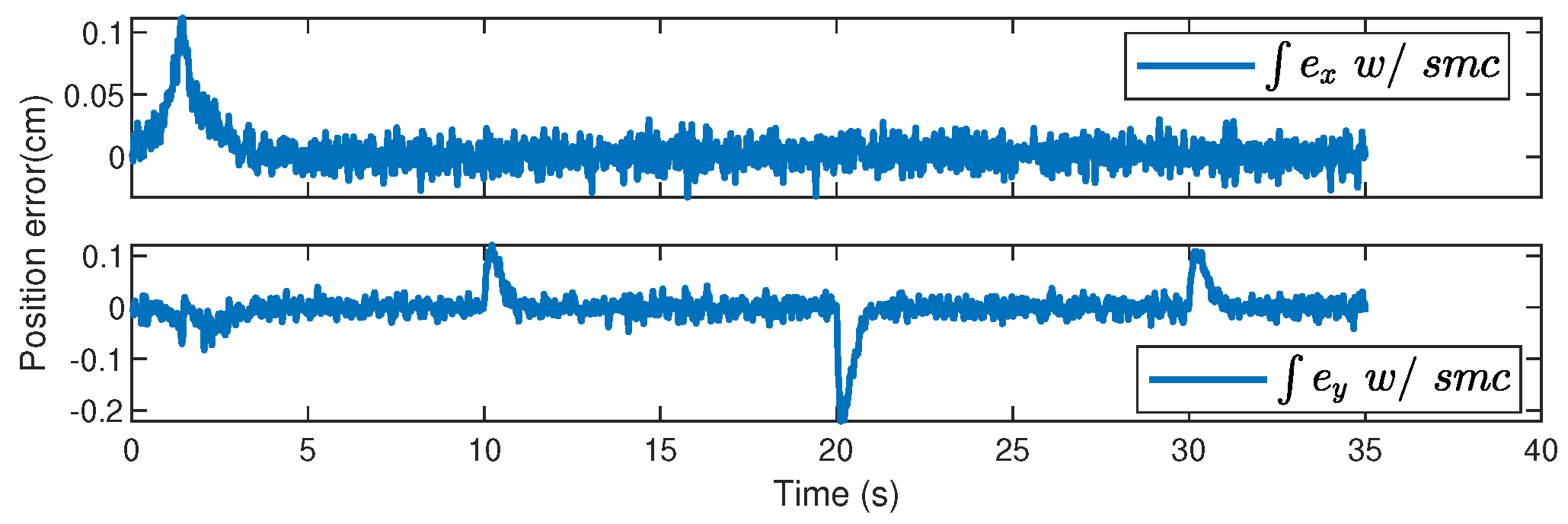
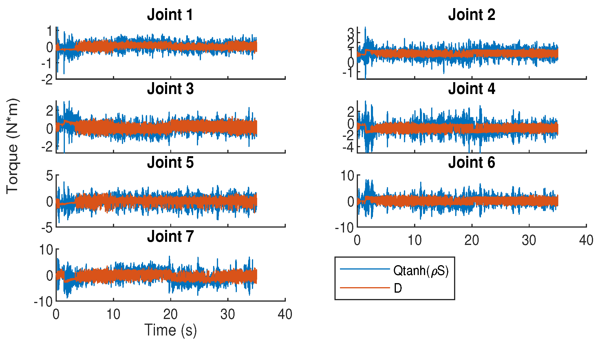
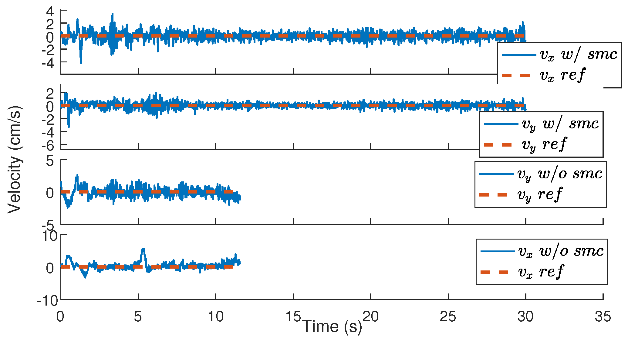
From Figure 10, Figure 11, Figure 12, Figure 13 and Figure 14, we can see similar performance as obtained with the frictionless environment. The force error in the z-axis is regulated within 0.5 N. The force in the y-axis is the friction force from the environment surface. The quaternion error is also regulated to within 0.01, which means that the relative attitude between the end-effector z-axis and environment normal converges to . Alignment results from Figure 13 show that the misalignment angle converges to 0. The velocity and position tracking in the x- and y-axes also perform as expected and the tracking error is regulated to within 0.2 cm. From Figure 14, we can see that the sliding mode control signal compensates for the disturbance, thereby converging the system dynamics to the desired dynamics.
6. Experiment
6.1. Implementation
For experimentation, the Baxter robot from Rethink Robotics was used as the testbed. The ATI Mini45 force/torque sensor was mounted on the wrist of the Baxter to sense the interaction force/torque. The sensor was covered with soft rubber to lower the stiffness of the end-tool. As for the signal processing, we utilized an averaging filter with a 45-sample window on the Baxter status publish node. For ease of implementation, we modified the controllers (16) and (61) as follows:
where is a constant diagonal matrix, while and denote desired rotational inertia and damping matrices.
6.2. Experimental Results
The following experiments were conducted: (1) alignment of the end-effector with a yoga ball, (2) moving the end-effector along the yoga ball, and (3) moving the end-effector along the back of a mannequin.
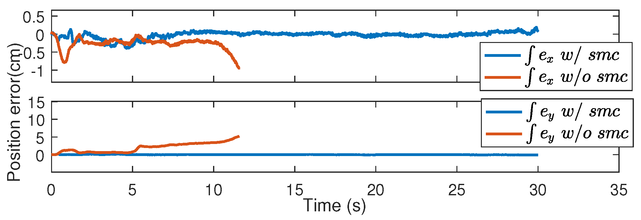
The first experiment focused on the alignment and stabilization of the end-effector with respect to the environment in order to highlight the critical role of sliding mode control (SMC). Here, we commanded 0 cm/s desired x and y velocities to the end-effector and as the desired force in the end-effector z-direction. From Figure 15, Figure 16, Figure 17, Figure 18 and Figure 19, it can be seen that use of SMC leads to the interaction force along the end-effector z-direction being regulated to around 10N with error while the position error was less than 0.2 cm after the end-effector aligned with the surface. The figures also show that the system does not converge without application of SMC. The interaction torque was seen to decrease to less than , and the equivalent lever converged to around 0.3 mm; both results clearly illustrate that the end-effector aligned along the yoga ball surface with high fidelity through the course of the experiment.
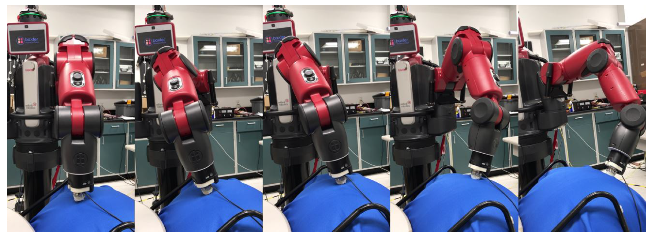
In the second experiment, we commanded as the desired force in the end-effector z-direction and the desired velocity was set to 0 from 0–10 s for the initial alignment and ±1.5 cm/s along the end-effector x-direction during the movement. The movement of the manipulator is shown in Figure 20.
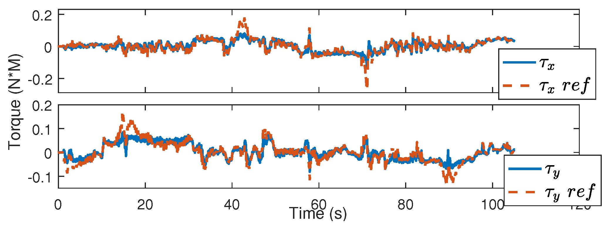
From Figure 21, Figure 22, Figure 23, Figure 24 and Figure 25, it can be seen that the force along the end-effector z-direction was regulated around 10 N while moving on the yoga ball with the desired velocity/position. It can be noticed that there was a minuscule torque error on the pitch axis of around during movement. Since the controller design assumes a level environment, this torque error drives the end-effector to perform a constant angular velocity to align with the curvature of the surface during the movement.
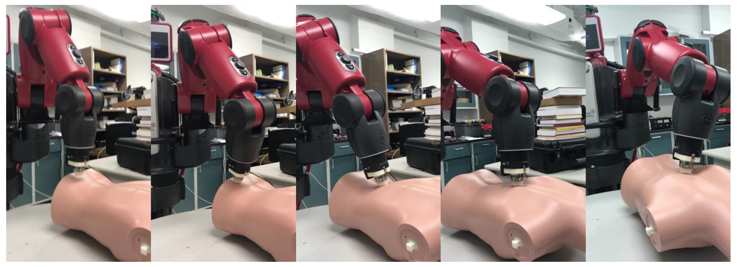
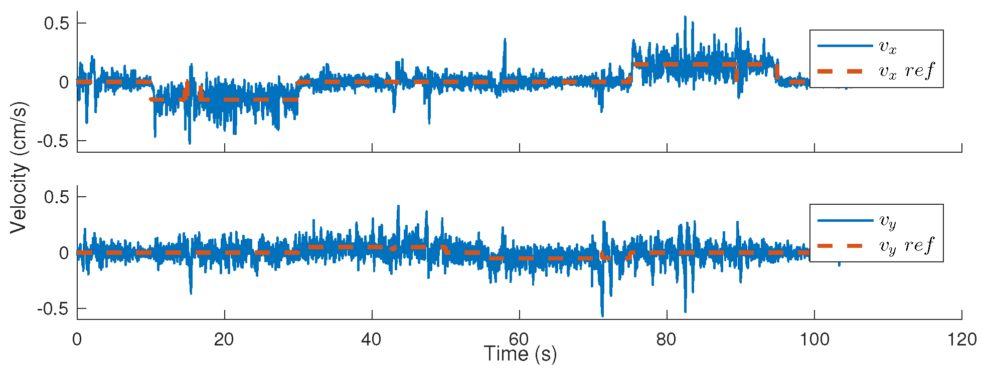
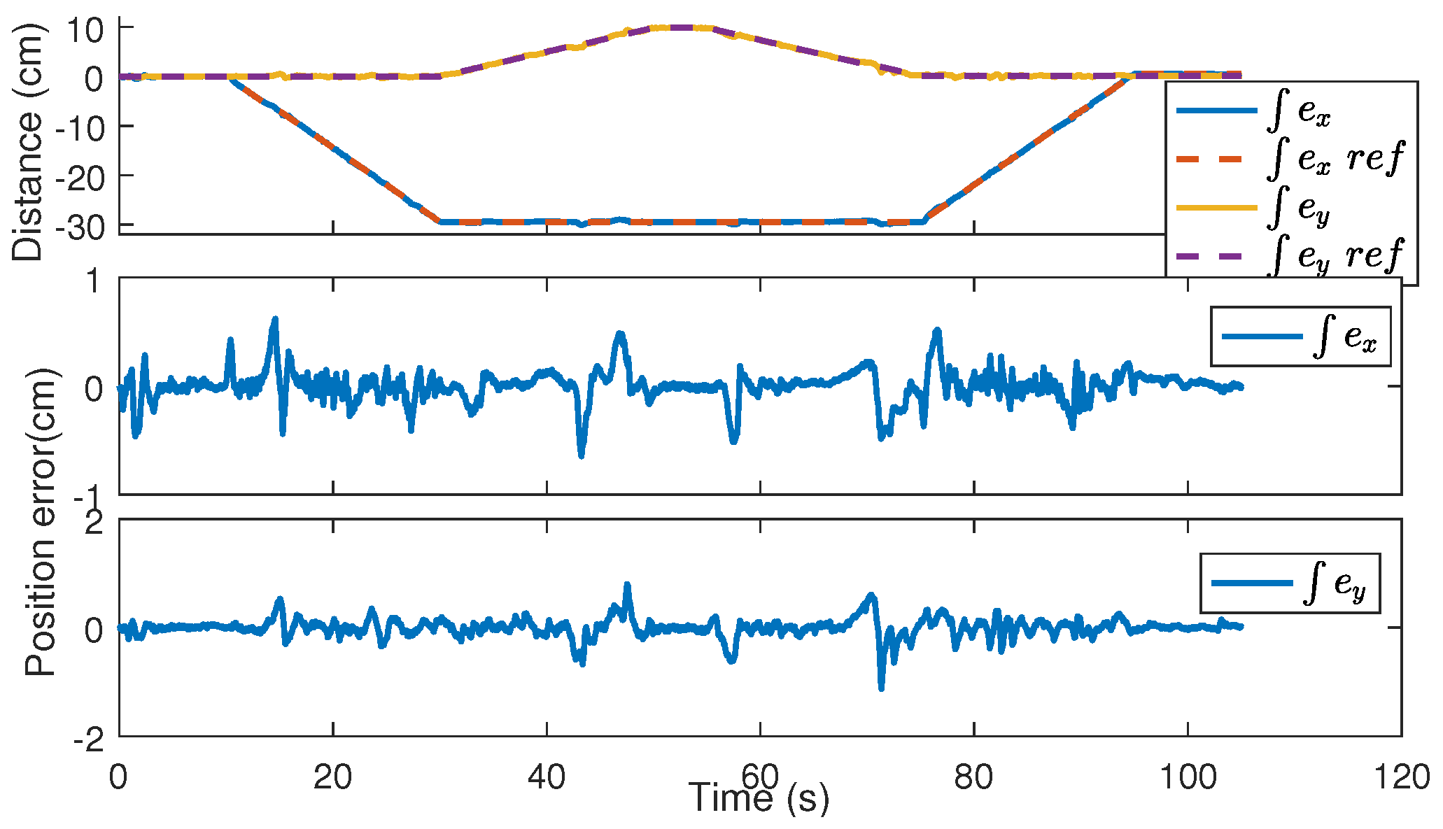
For the third experiment, we replaced the ball environment with a mannequin with an irregular surface typical of the back of a human torso. The movement of the manipulator is shown in Figure 26. From 0 to 10 s, we commanded the same force along the end-effector z-direction. Then, we set for 10–30 s, , for 30–50 s, , for 50–55 s, and then commanded the same velocities in the opposite direction. From Figure 27, Figure 28, Figure 29, Figure 30 and Figure 31, it can be seen that the overall position/velocity tracking and force regulation performance was close to expected. However, the performance was comparatively degraded with respect to the results in the second experiment due to the high stiffness and the sharp curvature changes in the surface of the mannequin. During the time periods when the end-effector moved over the sharp curvature regions on the mannequin back, such as 13–18 s, 40–45 s, 70–73 s, and 88–93 s, the force tracking and position tracking and alignment were affected. The force in the end-effector z-direction reduced to 4 N for about 0.1 s, the position error increased to 0.6 cm, the equivalent lever also increased to between 1 and cm, but the degradation was seen to happen for short periods and the force and position/velocity tracking profiles recovered each time.
7. Conclusions
In this paper, a robust hybrid controller has been implemented relying on the wrist force/torque and robot joint position/velocity feedback. A Lyapunov-based stability analysis is provided to prove both the convergence as well as passivity of the interaction to ensure both performance and safety. Simulations as well as experimental results verify the performance and robustness of the proposed impedance controller in the presence of dynamic uncertainties as well as the safety compliance of physical human–robot interactions for a redundant robot manipulator. The design and implementation of verifiably safe PHRI controllers is important for deploying such controllers in the real world without the need for specialized hardware (sensors and/or actuators), which can be expensive. This is especially important for assistive robotics applications where cost is among the most critical factors in technology adoption. Our future work will be focused on adapting impedance parameters during interaction to limit force amplitudes.
Author Contributions
Conceptualization, A.B.; methodology, A.B.; software, Z.D. and M.B.; validation, Z.D. and M.B.; formal analysis, Z.D.; investigation, Z.D.; resources, A.B.; writing—original draft preparation, Z.D.; writing—review and editing, A.B.; visualization, Z.D.; supervision, A.B.; project administration, A.B.; funding acquisition, A.B. All authors have read and agreed to the published version of the manuscript.
Funding
This study was funded in part by NIDILRR grant #H133G120275, and in part by NSF grant numbers IIS-1409823 and IIS-1527794. However, these contents do not necessarily represent the policy of the aforementioned funding agencies, and you should not assume endorsement by the Federal Government.
Data Availability Statement
Not applicable.
Conflicts of Interest
The authors declare no conflict of interest.
Appendix A
Appendix A.1. Definition and Growth Bound of G1(t)
The time derivative of (42) can be written as
where we have utilized (42) and (43) to substitute for as well as the identity that . By utilizing the identity that , we can simplify
where
and
which can be bounded as
which is an exponential bound owing to the exponential boundedness for q from Lemma 2. By decomposing as
we can rewrite the perturbation system (A1) as follows
where
The denominator term in and can be lowerbounded as follows:
since and converges exponentially to 1. Since and H converge exponentially to the origin, we can upperbound as follows:
where are system-parameter-dependent constants.
Appendix A.2. Definitions of A, P and Q
The matrices A, P, and Q are defined as follows:
for sufficiently small .
Appendix A.3. Definition and Linear Growth Bound of G2(t)
Appendix A.4. Bound for
Appendix A.5. Exponential Convergence of to Implies Exponential Convergence of θc to θd
Based on the relation between , and , , we can write
Since and , it is easy to see that all the bracketed terms in (A9) can be bounded by constants such that
which clearly shows that the exponential convergence of to the origin implies the same convergence result for
References
- Engelberger, J. Robotics in Service; The MIT Press: Cambridge, MA, USA, 1989. [Google Scholar]
- Kwee, H.H.; Duimel, J.J.; Smits, J.J.; Tuinhof de Moed, A.A.; van Woerden, J.A. The MANUS Wheelchair-Borne Manipulator: System Review and First Results. In Proceedings of the IARP Workshop on Domestic and Medical & Healthcare Robotics, Newcastle, UK, 1989; pp. 385–395. [Google Scholar]
- Van der Loos, M.; Michalowski, S.; Leifer, L. Design of an Omnidirectional Mobile Robot as a Manipulation Aid for the Severely Disabled. In Interactive Robotic Aids, World Rehabilitation Fund Monograph #37; Foulds, R., Ed.; World Rehabilitation Fund: New York, NY, USA, 1986. [Google Scholar]
- Mahoney, R.M. The Raptor Wheelchair Robot System. In Integration of Assistive Technology in the Information Age; Mokhtari, M., Ed.; IOS: Amsterdam, The Netherlands, 2001; pp. 135–141. [Google Scholar]
- Prior, S.D. An electric wheelchair mounted robotic arm—A survey of potential users. J. Med. Eng. Technol. 1990, 14, 143–154. [Google Scholar] [CrossRef] [PubMed]
- Nguyen, H.; Anderson, C.; Trevor, A.; Jain, A.; Xu, Z.; Kemp, C. El-E: An Assistive Robot that Fetches Objects from Flat Surfaces. In Proceedings of the Human-Robot Interaction 2008 Workshop on Robotic Helpers, Amsterdam, The Netherlands, 12 March 2008. [Google Scholar]
- Bien, Z.; Kim, D.-J.; Chung, M.J.; Kwon, D.S.; Chang, P.H. Development of a Wheelchair-Based Rehabilitation Robotic System (KARES II) with Various Human Robot Interaction Interfaces for the Disabled. In Proceedings of the IEEE/ASME International Conference on Advanced Intelligent Mechatronics, Kobe, Japan, 20–24 July 2003; pp. 902–907. [Google Scholar]
- Neveryd, H.; Bolmsj, G. WALKY, an Ultrasonic Navigating Mobile Robot for the Disabled. In Proceedings of the TIDE, Paris, France, 26–28 April 1995; pp. 366–370. [Google Scholar]
- Dario, P.; Guglielmelli, E.; Laschi, C.; Teti, G. Movaid: A Mobile Robotic System Residential Care to Disabled and Elderly People. In Proceedings of the First MobiNet Symposium, Athens, Greece, 1997; pp. 9–14. [Google Scholar]
- Bischoff, R. Design, Concept, and Realization of the Humanoid Service Robot HERMES. In Field and Service Robotics; Zelinsky, A., Ed.; Springer: London, UK, 1998; pp. 485–492. [Google Scholar]
- Ding, Z.; Paperno, N.; Prakash, K.; Behal, A. An Adaptive Control-Based Approach for 1-Click Gripping of Novel Objects Using a Robotic Manipulator. IEEE Trans. Control Syst. Technol. 2019, 27, 1805–1812. [Google Scholar] [CrossRef]
- Al-Mohammed, M.; Adem, R.; Behal, A. A Switched Adaptive Controller for Robotic Gripping of Novel Objects With Minimal Force. IEEE Trans. Control Syst. Technol. 2023, 31, 17–26. [Google Scholar] [CrossRef]
- Kim, D.; Wang, Z.; Behal, A. Motion Segmentation and Control Design for UCF-MANUS—An Intelligent Assistive Robotic Manipulator. IEEE/ASME Trans. Mechatron. 2012, 17, 936–948. [Google Scholar] [CrossRef]
- Nagata, F.; Hase, T.; Haga, Z.; Omoto, M.; Watanabe, K. CAD/CAMbased Position/Force Controller for a Mold Polishing Robot. Mechatronics 2007, 17, 207–216. [Google Scholar] [CrossRef]
- King, C.; Chen, T.L.; Jain, A.; Kemp, C.C. Towards an assistive robot that autonomously performs bed baths for patient hygiene. In Proceedings of the 2010 IEEE/RSJ International Conference on Intelligent Robots and Systems, Taipei, Taiwan, 18–22 October 2010; pp. 319–324. [Google Scholar]
- Hawkins, K.P.; King, C.H.; Chen, T.L.; Kemp, C. Informing assistive robots with models of contact forces from able-bodied face wiping and shaving. In Proceedings of the RO-MAN, Paris, France, 9–13 September 2012; pp. 251–258. [Google Scholar]
- Jamisola, R.S.; Kormushev, P.; Bicchi, A.; Caldwell, D.G. Haptic exploration of unknown surfaces with discontinuities. In Proceedings of the 2014 IEEE/RSJ International Conference on Intelligent Robots and Systems, Chicago, IL, USA, 14–18 September 2014; pp. 1255–1260. [Google Scholar]
- Gracia, L.; Solanes, J.E.; Muz-Benavent, P.; Miro, J.V.; Perez-Vidal, C.; Tornero, J. Adaptive Sliding Mode Control for Robotic Surface Treatment Using Force Feedback. Mechatronics 2018, 52, 102–118. [Google Scholar] [CrossRef]
- Roveda, L.; Vicentini, F.; Tosatti, L.M. Deformation-tracking impedance control in interaction with uncertain environments. In Proceedings of the 2013 IEEE/RSJ International Conference on Intelligent Robots and Systems, Tokyo, Japan, 3–7 November 2013; pp. 1992–1997. [Google Scholar]
- Moura, J.; Mccoll, W.; Taykaldiranian, G.; Tomiyama, T.; Erden, M.S. Automation of Train Cab Front Cleaning With a Robot Manipulator. IEEE Robot. Autom. 2018, 3, 3058–3065. [Google Scholar] [CrossRef] [Green Version]
- Ding, Z. Robust Impedance Control Design of a Robot Manipulator for Passive Physical Human-Robot Interaction. Available online: https://youtu.be/IAccCLQKWuY (accessed on 12 August 2023).
- Feng, Y.; Yu, X.; Man, Z. Non-singular terminal sliding mode control of rigid manipulators. Automatica 2002, 38, 2159–2167. [Google Scholar] [CrossRef]
- Behal, A.; Dixon, W.E.; Dawson, D.M.; Xian, B. Lyapunov-Based Control of Robotic Systems; CRC Press: Boca Raton, FL, USA, 2009; ISBN 0-8493-7025-6. [Google Scholar]
- Khalil, H.K. Nonlinear Systems, 3rd ed.; Prentice Hall: Upper Saddle River, NJ, USA, 2002. [Google Scholar]
- Tayebi, A.; McGilvray, S. Attitude stabilization of a VTOL quadrotor aircraft. IEEE Trans. Control Syst. Technol. 2006, 14, 562–571. [Google Scholar] [CrossRef] [Green Version]
Figure 1.
Spring-damper environmental model.

Figure 2.
End-tool geometry, where and are the spring- and damper-induced forces from the environment.
Figure 2.
End-tool geometry, where and are the spring- and damper-induced forces from the environment.

Figure 3.
Block diagram of proposed physical human–robot interaction controller.

Figure 4.
External force profile.

Figure 5.
Velocity tracking profile.

Figure 6.
Position tracking profile.

Figure 7.
Quaternion tracking profile.

Figure 8.
Misalignment evaluation: (Top) Misalignment angle between the end-effector z-direction and the normal of the contact surface. (Bottom) Equivalent lever in end-effector tangential direction.
Figure 8.
Misalignment evaluation: (Top) Misalignment angle between the end-effector z-direction and the normal of the contact surface. (Bottom) Equivalent lever in end-effector tangential direction.

Figure 9.
Geometry of the end-tool. Left plot is the general misalignment case for the environment with friction. Middle plot is the equilibrium of the controller in last section applied to the frictional environment. The right plot is the desired equilibrium for the frictional environment.
Figure 9.
Geometry of the end-tool. Left plot is the general misalignment case for the environment with friction. Middle plot is the equilibrium of the controller in last section applied to the frictional environment. The right plot is the desired equilibrium for the frictional environment.

Figure 10.
Force tracking profile for frictional environment.

Figure 11.
Quaternion error tracking profile for frictional environment.

Figure 12.
Velocity tracking profile for frictional environment.

Figure 13.
Alignment evaluation for frictional environment.

Figure 14.
SMC performance for frictional environment.

Figure 15.
External force for ball alignment.

Figure 16.
External torque for ball alignment.

Figure 17.
Velocity tracking for ball environment alignment experiment.

Figure 18.
Position tracking and error for ball environment alignment experiment.

Figure 19.
Alignment evaluation for ball environment alignment.

Figure 20.
Video frames from the experiment on the yoga ball environment.

Figure 21.
External force for moving on ball environment.

Figure 22.
External torque profile for moving on ball environment.

Figure 23.
Velocity tracking for moving on ball environment.

Figure 24.
Position tracking for moving on ball environment.

Figure 25.
Alignment evaluation for moving on ball environment.

Figure 26.
Video frames from the experiment on the mannequin environment.

Figure 27.
External force profile for moving on mannequin back. During initial alignment (0–10 s), force error is less than 0.5 N. During movement, force error stays less than 2 N except when end-effector moves on regions of sharp curvature where force error goes to 4 N for less than 0.2 s.
Figure 27.
External force profile for moving on mannequin back. During initial alignment (0–10 s), force error is less than 0.5 N. During movement, force error stays less than 2 N except when end-effector moves on regions of sharp curvature where force error goes to 4 N for less than 0.2 s.

Figure 28.
External torque profile for moving on mannequin. To orient end-effector during changes in surface curvature, torque error increases up to 0.1 Nm, otherwise it remains regulated to within 0.05 Nm.
Figure 28.
External torque profile for moving on mannequin. To orient end-effector during changes in surface curvature, torque error increases up to 0.1 Nm, otherwise it remains regulated to within 0.05 Nm.

Figure 29.
Velocity tracking for moving on mannequin back.

Figure 30.
Position tracking and error profile for moving on mannequin back.

Figure 31.
Equivalent lever in the tangential plane of end-effector. At 13 s, 41 s, 70 s, and 88 s, end-effector moves on regions of sharp curvature on mannequin which affects alignment during the transient, but the controller always recovers alignment in steady-state.
Figure 31.
Equivalent lever in the tangential plane of end-effector. At 13 s, 41 s, 70 s, and 88 s, end-effector moves on regions of sharp curvature on mannequin which affects alignment during the transient, but the controller always recovers alignment in steady-state.


Table 1.
Simulation parameters.
Disclaimer/Publisher’s Note: The statements, opinions and data contained in all publications are solely those of the individual author(s) and contributor(s) and not of MDPI and/or the editor(s). MDPI and/or the editor(s) disclaim responsibility for any injury to people or property resulting from any ideas, methods, instructions or products referred to in the content. |
© 2023 by the authors. Licensee MDPI, Basel, Switzerland. This article is an open access article distributed under the terms and conditions of the Creative Commons Attribution (CC BY) license (https://creativecommons.org/licenses/by/4.0/).
Share and Cite
MDPI and ACS Style
Ding, Z.; Baghbahari, M.; Behal, A. A Passivity-Based Framework for Safe Physical Human–Robot Interaction. Robotics 2023, 12, 116. https://doi.org/10.3390/robotics12040116
AMA Style
Ding Z, Baghbahari M, Behal A. A Passivity-Based Framework for Safe Physical Human–Robot Interaction. Robotics. 2023; 12(4):116. https://doi.org/10.3390/robotics12040116
Chicago/Turabian StyleDing, Zhangchi, Masoud Baghbahari, and Aman Behal. 2023. "A Passivity-Based Framework for Safe Physical Human–Robot Interaction" Robotics 12, no. 4: 116. https://doi.org/10.3390/robotics12040116
Note that from the first issue of 2016, this journal uses article numbers instead of page numbers. See further details here.