

A Hybrid Motion Planning Algorithm for Multi-Mobile Robot Formation Planning
by
 , and
, and
Haojie Chen
1,
Zifan Wang
1,
Xiaoxu Liu
1,
Wenke Ma
2,
Qiang Wang
2,
Wenjun Zhang
3 and
Tan Zhang
1,* 1
College of Sino-German Intelligent Manufacturing, Shenzhen Technology University, 3002 Lantian Road, Shenzhen 518118, China
2
Shenzhen Research Institute of Northwestern Polytechnical University, 45 Gaoxin South 9th Road, Shenzhen 518057, China
3
Department of Mechanical Engineering, University of Saskatchewan, 57 Campus Drive, Saskatoon, SK S7N5A9, Canada
*
Author to whom correspondence should be addressed.
Robotics 2023, 12(4), 112; https://doi.org/10.3390/robotics12040112
Submission received: 19 June 2023
/
Revised: 24 July 2023
/
Accepted: 27 July 2023
/
Published: 4 August 2023
(This article belongs to the Special Issue The State-of-the-Art of Robotics in Asia)
Abstract
:This paper addresses the problem of relative position-based formation planning for a leader–follower multi-robot setup, where the robots adjust the formation parameters, such as size and three-dimensional orientation, to avoid collisions and progress toward their goal. Specifically, we develop a virtual sub-target-based obstacle avoidance method, which involves a transitional virtual sub-target that guides the robots to avoid obstacles according to obstacle information, target, and boundary. Moreover, we develop a changing formation strategy to determine the necessity to avoid collisions and a priority-based model to determine which robots move, thus dynamically adjusting the relative distance between the followers and the leader. The backstepping-based sliding motion controller guarantees that the trajectory and velocity tracking errors converge to zero. The proposed robot navigation method can be employed in various environments and types of obstacles, allowing for a formation change. Furthermore, it is efficient and scalable under various numbers of robots. The approach is experimentally verified using three real mobile robots and up to five mobile robots in simulated scenarios.
1. Introduction
The multi-robot formation has been widely used in multi-robots [1], surface vessels [2], and satellites [3]. Formation planning is a multi-agent architecture that relies on the agents’ relative motion [4], aiming to maintain a specified geometrical shape of a robotic group by adjusting the agents’ pose [5], following the formation-forming, maintaining, and switching process.
The control community suggests various approaches to ensure formation planning for multi-agent systems, namely behavior-based [6], virtual structure-based [7], and leader–follower-based [8]. In the behavior-based approaches, each agent of the formation acts according to some predefined behavior, which limits its motion options. The virtual structure-based approach introduces a virtual vehicle for each actual vehicle in the formation and transforms the formation problem into a trajectory-tracking problem. Since the virtual vehicles are not exposed to environmental disturbance, the followers usually break the formation in unexpected real environmental disturbances. The leader–follower-based formation planning with unknown obstacles involves controlling multi-mobile robots to maintain a certain geometric formation, aiming to collaboratively complete the obstacle avoidance task. Although the leader–follower approach is easy to implement and all agents react to any environmental change, the network delay must be considered to maintain the formation. Multi-robot formation control, collision, and obstacle avoidance are big challenges due to their uncontrollability and complexity, with only a few works considering collision-free obstacle avoidance during a changing robotic formation.
In [9], the authors combined flocking with distance-based shape control using the steepest descent formation planning method, which is appropriate for a multi-agent system to achieve formation planning. The artificial potential field (APF) method features a simpler controller and involves fewer parameters and therefore has been widely used for real-time formation control [10] and collision and obstacle avoidance [11]. The work in [12] proposed a method based on a finite control set model predictive method to solve the formation collision. The work in [13] proposed a potential field-based formation control approach for agents, enabling them to achieve formation control by regulating their relative positions. In [14], the authors combined the leader–follower formation approach and the APF method to address the formation control problem with obstacle avoidance. However, the authors did not consider the local minimum of the potential function in a complex environment. Considering the agent’s dimensions, a repulsive potential function was proposed to solve the problem of avoiding a local minimum solution [15], where a modified artificial goal technique and several virtual obstacle methods were developed to avoid obstacles. However, the methods above analyze the local minimum of one agent, ignoring the formation control and collision avoidance.
Therefore, this paper proposes a formation planning method for online obstacle avoidance. Compared with state-of-the-art approaches, the contributions of this work are as follows:
- In obstacle avoidance planning, the leader robot plans a safe path using the virtual goal control method.
- Based on the new desired distances and bearing angles, we design a priority model where the follower robots change the formation to avoid obstacles exploiting the desired distance and bearing angles between the leader and follower robots.
We propose a tracking control algorithm based on Backstepping and Sliding Motion to guarantee that the trajectory and velocity tracking errors converge to zero.
2. Kinematics Model
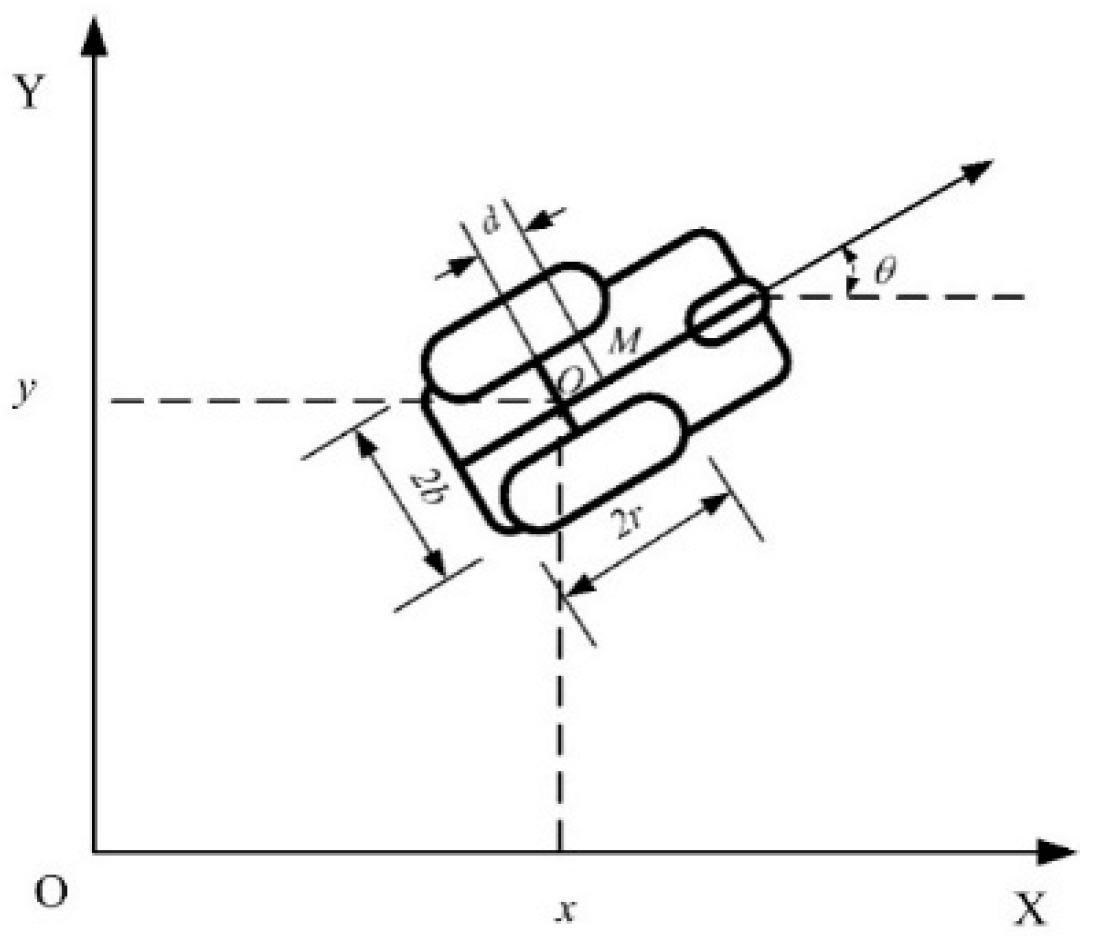
Figure 1 illustrates the kinematics model of a wheeled mobile robot comprising two coaxial driving rear wheels and an auxiliary front wheel, where O is the geometric center point of the line connecting the left and right wheels of the robot, and M is the mass point of the robot. Let vector represent the robot’s pose in the generalized coordinate system XOY, where are the coordinates of the center point O, and is the angle between the moving direction of the robot and the horizontal line.
The robot can only move in the direction perpendicular to the drive wheel axis and must meet the conditions of pure rolling and no sliding. The nonholonomic constraints on this robot are as follows:
The robot’s kinematic model is:
where v denotes the linear velocity of the mobile robot and w is the angular velocity of the mobile robot. This work considers , i.e., the robot’s geometric center coincides with the center of mass.
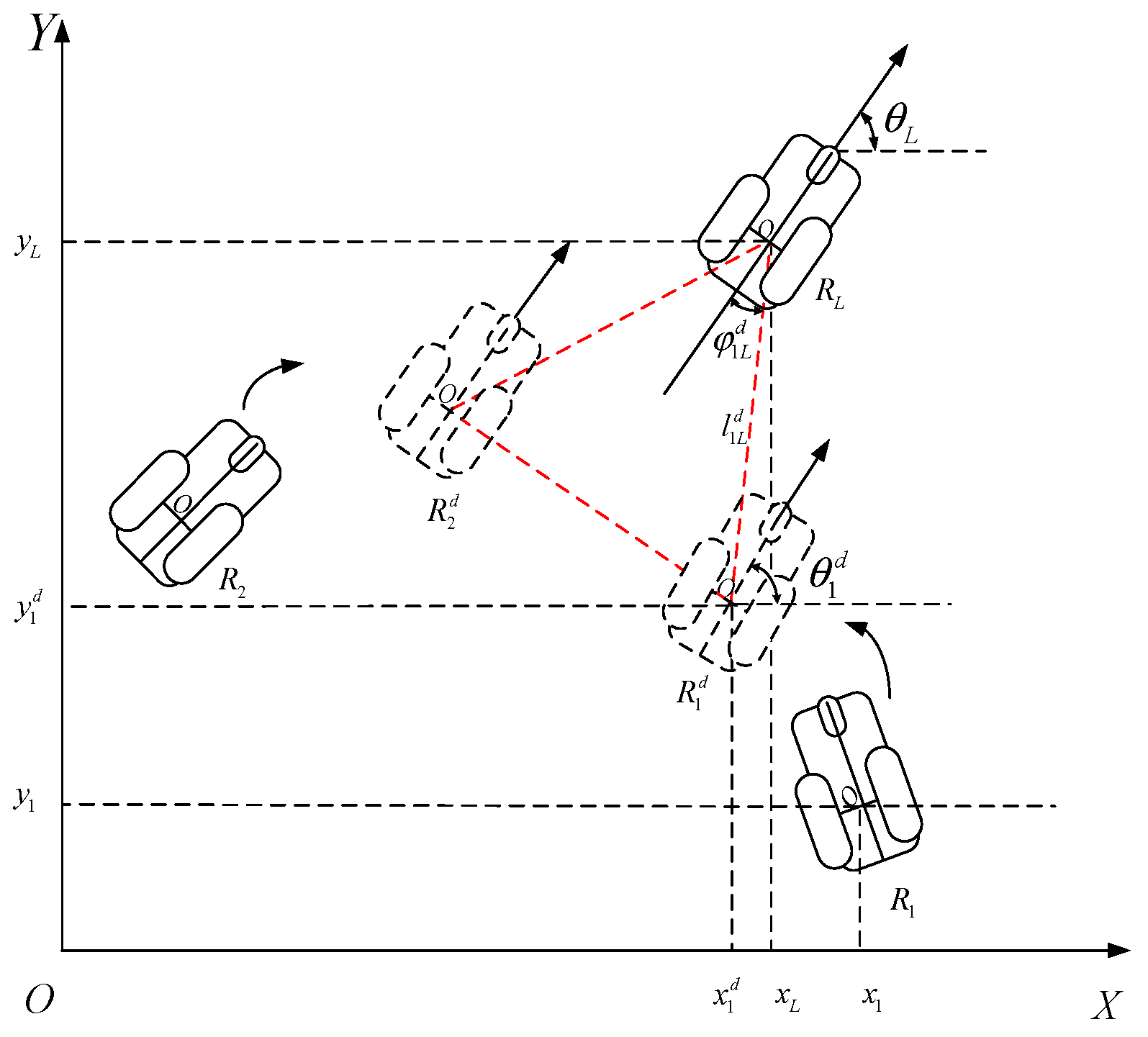
Leader–Follower Formation Kinematics Model
Figure 2 depicts the kinematics model of the leader–follower formation. The leader is responsible for the formation’s main trajectory and determines its overall direction online. The following robots form a formation by tracking the virtual robot (see the dotted line). The ideal pose of the follower is as follows:
where is the ideal pose of the ith follower, is the pose of the leader, and and are the distance and angle during formation. The actual pose of the robot is , and the tracking pose error of the follower is as follows:
where is the error between the follower and its ideal pose. Thus, the goal of the formation planning is to minimize the tracking error.
3. Leader–Follower Formation Planning
The leader–follower formation refers to the leader robot leading the follower robot to obtain obstacle information online (moving and stationary obstacles) using its sensors. Based on that information, a series of key points are planned, creating an obstacle-avoidance path for the entire formation. The leader robot leads the formation to track the target point and is responsible for perceiving the unknown environment and identifying the obstacles that must be avoided. The online motion planning of the leader–follower formation is conducted under certain constraints and assumptions: (1) the formation is formed before the obstacle is detected, (2) the formation already knows the final destination point, and (3) the formation has no communication delay, no signal loss, and no mechanical failure.
3.1. Virtual Sub-Goal-Based Motion Planning
When a single obstacle must be avoided, the leader establishes a series of virtual transition sub-goals in real time based on the sensor information obtained and the boundary of a single obstacle. Then, the leader guides the formation to avoid obstacles. When multiple obstacles must be avoided, the robot establishes a series of virtual transition sub-targets in real time based on the sensor information and the position of the target point by exploiting the inner and outer boundaries of the two obstacles closer to the target point. Following that, the leader guides the formation to avoid obstacles. Although the traditional artificial potential field (APF) solves the real-time formation path planning problem without global map information, it is prone to oscillation and wandering between narrow and long areas of multiple obstacles. Thus, this paper uses the “virtual sub-goal” strategy that adds online virtual sub-goals to the leader robot in an unknown environment.
3.1.1. Online Motion Planning with A Single Obstacle
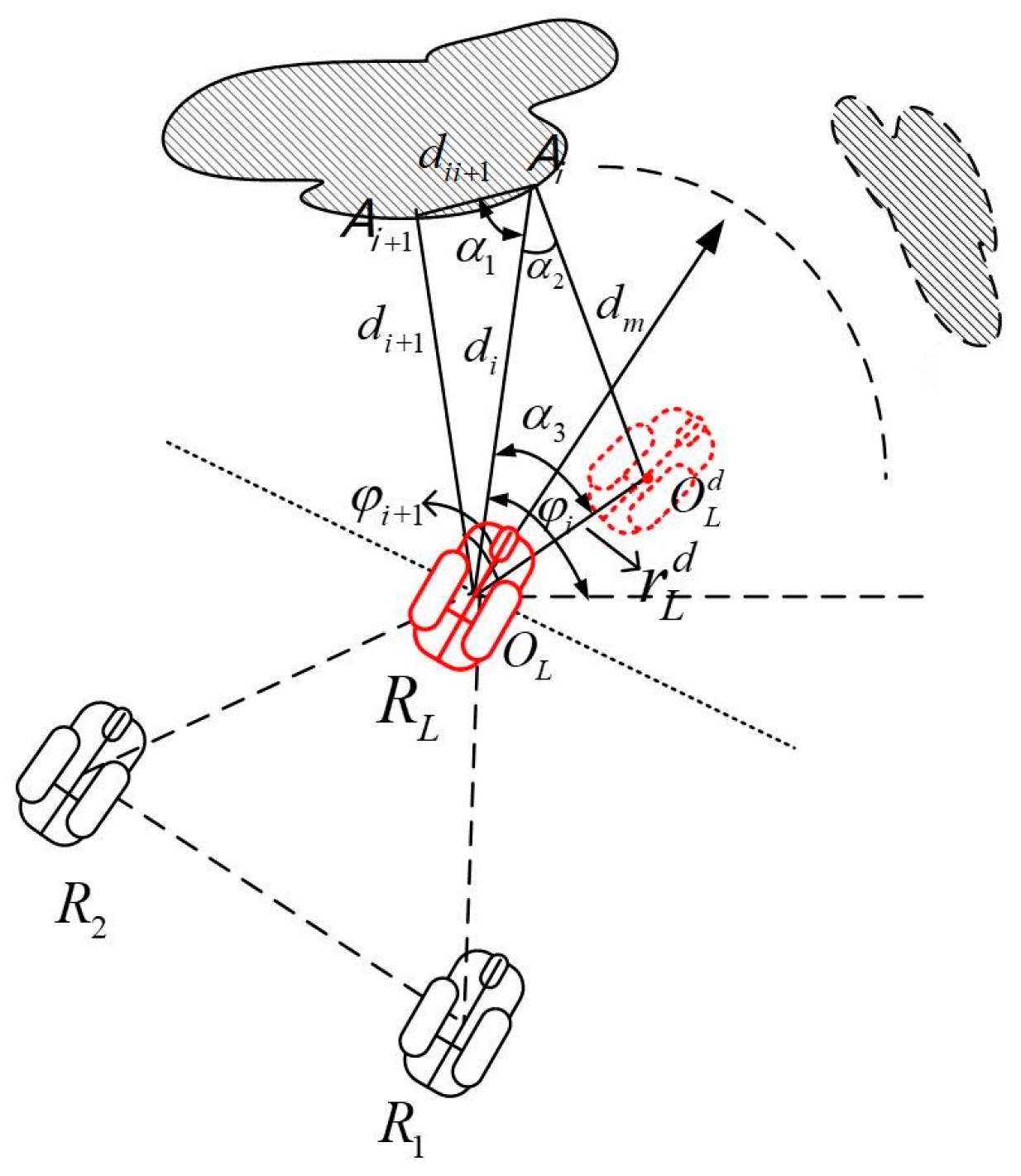
Suppose the leader robot encounters a single obstacle in the detection area. In that case, the passable area from the current position to the target point is obtained by calculating the sensor output of the target-obstacle distance information. This is illustrated in Figure 3, where the red-dotted robot is the virtual sub-target of the leader robot at the next moment, and its position coordinates are calculated through the process presented next.
Specifically, first, the leader robot obtains the real-time distance between two adjacent points on the obstacle to be avoided and calculates and angle between the target and the beam close to the moving direction of the robot. The robot conducts obstacle avoidance planning in its forward direction.
where , is the angle between the adjacent points on the obstacle boundary that must be avoided at time and the horizontal line. , is the distance between the point on the boundary of the obstacle that must be avoided at time and the leader robot.
During the robot’s motion, if the boundary of an obstacle is too small, i.e., if and only if the only light beam emitted along the direction of the robot’s movement detects the obstacle and its angle is perpendicular to the boundary of the obstacle, the robot cannot judge where to move at the next moment, forcing the robot to stop. To avoid this situation, we added a very small disturbance item .
Equation (7) assists the leader robot in approaching point where the red solid line robot is located in Figure 3 and moves where the red dashed robot is located at . The distance traveled is:
where is a positive value related to the formation, set to a small number.
Next, we found the angle that the leader robot must deviate from beam , and the angle in Figure 3 was calculated as follows:
According to Equation (5), the virtual sub-goal of the leader robot at the next moment is finally obtained as follows:
The ideal angle to set the leader robot for the next moment is as follows:
3.1.2. Online Motion Planning with Double Obstacles
When multiple obstacles must be avoided, the robot establishes a series of virtual sub-targets based on the obtained obstacle distribution information and the position of the target point to guide the formation to avoid obstacles. This process relies on the inner and outer boundaries of the two obstacles closer to the target point.
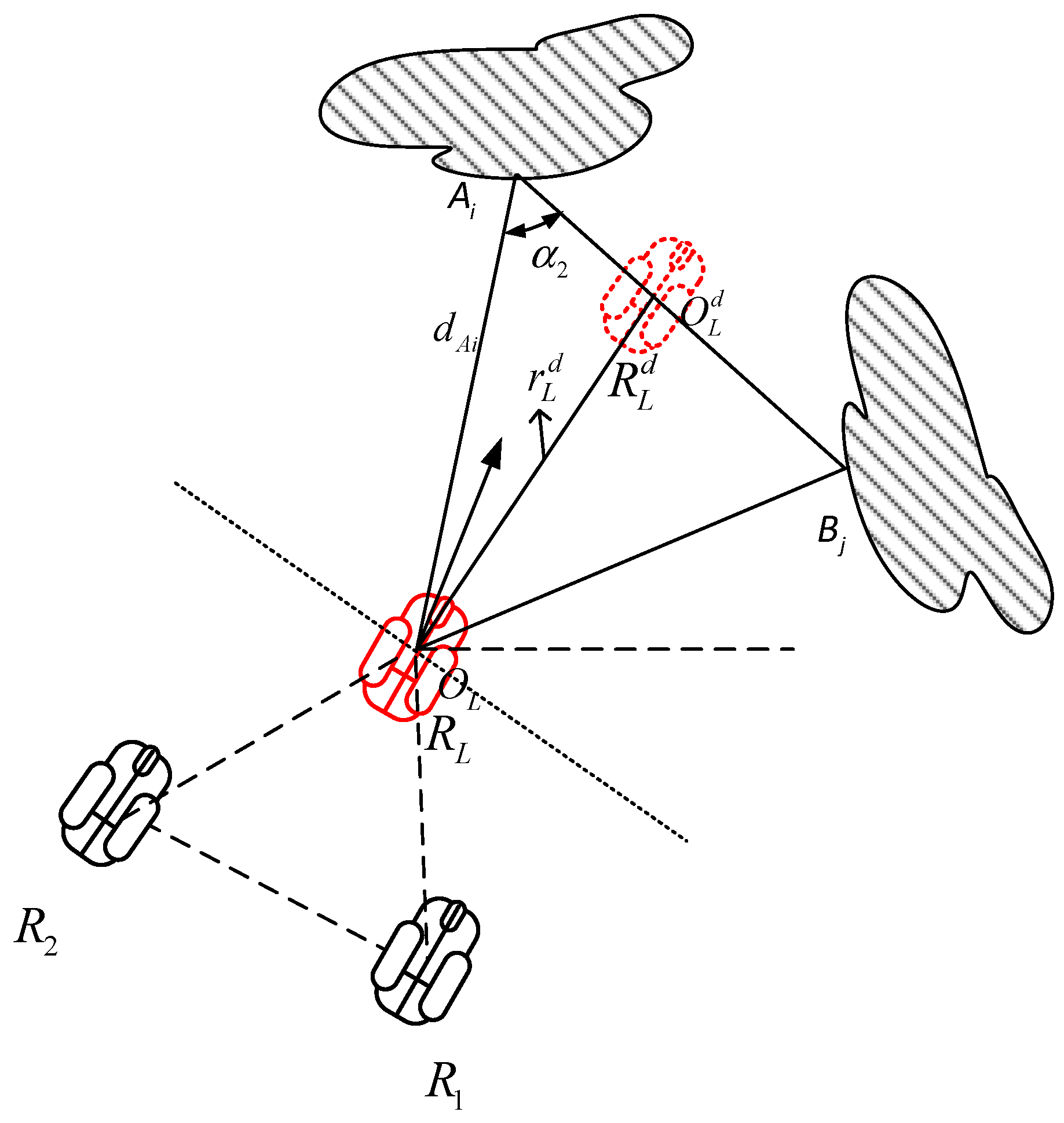
If the leader robot must avoid two obstacles, the leader’s moving direction is between the two obstacles, as depicted in Figure 4. According to the obstacle merging rules, the area between adjacent obstacles is sufficient for the leader robot to pass through and avoid the obstacles.
For the double obstacle scenario, the leader robot detects two points on the boundary of different obstacles that must be avoided , (see Figure 4). According to the detection results, online motion planning is conducted to obtain the virtual sub-target of the leader at the next moment, and the virtual sub-goal of the leader is specified for the next moment. Given the midpoint coordinates of used to solve the point coordinates, the following calculations need to be performed:
The distance between two points on the boundary of this double obstacle , is:
where , is the angle between the point on the boundary of the two obstacles to be avoided at time and the horizontal line. , is the distance between the points on the boundary of the two obstacles that must be avoided at time relative to the leader robot.
According to the relative distance information between the obstacle point and the leader robot, first, we find the angle between any beam on the obstacle and the figure . Following that,
The leader robot moves from the point where the red solid line robot is located in the figure to the point where the red dotted line robot is located in the figure , and the corresponding distance:
According to the angle and moving distance, we calculated the relative angle between the robot and a light beam, namely:
For the leader at the previous moment and the angle between the beam and the X-axis, the virtual sub-target of the leader at the next moment is calculated as follows:
Following that, the ideal angle that must be adjusted from the current position towards the virtual sub-goal is defined as follows:
So far, the obstacle avoidance path planning of the leader robot at two adjacent moments before and after was obtained under double obstacles.
3.2. Priority-Based Multi-Robot Motion Planning
The leader robot evaluates the distribution of the obstacle that must be avoided and then establishes a series of virtual sub-targets along the free area to guide the formation. The follower robots avoid the obstacles online according to the distribution of the obstacles defined by the leader and exploit the priority model to coordinate any internal collisions. This strategy is mainly used for double obstacle scenarios.
3.2.1. Collision Avoidance Coordination Based on the Priority Model
The follower robot in the formation compares , which is the distance between itself and the leader and the relative angle with the leader in real time. Following that, the priority of the follower robot is established, which involves the distance priority and angular priority. The following priority model is:
where and are the distance and angular priority of the following robot.
Moreover, the dynamic priority model includes the following steps (Algorithm 1):
(1) Determine the distance priority, compare the distance between each follower robot and the leader robot in the current state, and the priority of the smaller distance is higher.
(2) Determine the angular priority. When the distance is equal, determine the angle between the follower and leader robots. The counterclockwise direction is considered positive, and thus the angle is positive, and the priority is higher.
(3) Final judgment. When the signs of the included angles are the same, compare the absolute value of the included angle. The robot with the smaller absolute value has a higher priority.
| Algorithm 1: Algorithm of intra-group priority of the robot. |
| 1: Input: current formation distance , and current bearing angle , of the i, jth robot. |
| 2: if (), Update the priority Pi > Pj, |
| else |
| 3: if () and (), Update the priority Pi > Pj, else |
| 4: if (||<||), |
| Update the priority Pi > Pj, 5: end |
3.2.2. Online Motion Planning Based on Formation Adjustment Strategy
We propose an adjusting strategy before the robot formation to reduce the total computational burden to detect the necessity for collision avoidance. (1) If there is no collision, each follower robot preserves its position, which is only adjusted relatively to the leader robot. (2) Otherwise, the follower robot with high priority remains the same as the leader robot’s leader and only changes its relative azimuth with the leader robot to obtain the obstacle avoidance path point. The follower robot with low priority changes its position related to the formation leader and the relative azimuth with the leader robot and obtains the obstacle avoidance path point.
3.2.3. Online Motion Planning for the Follower Robot without Collision Problem
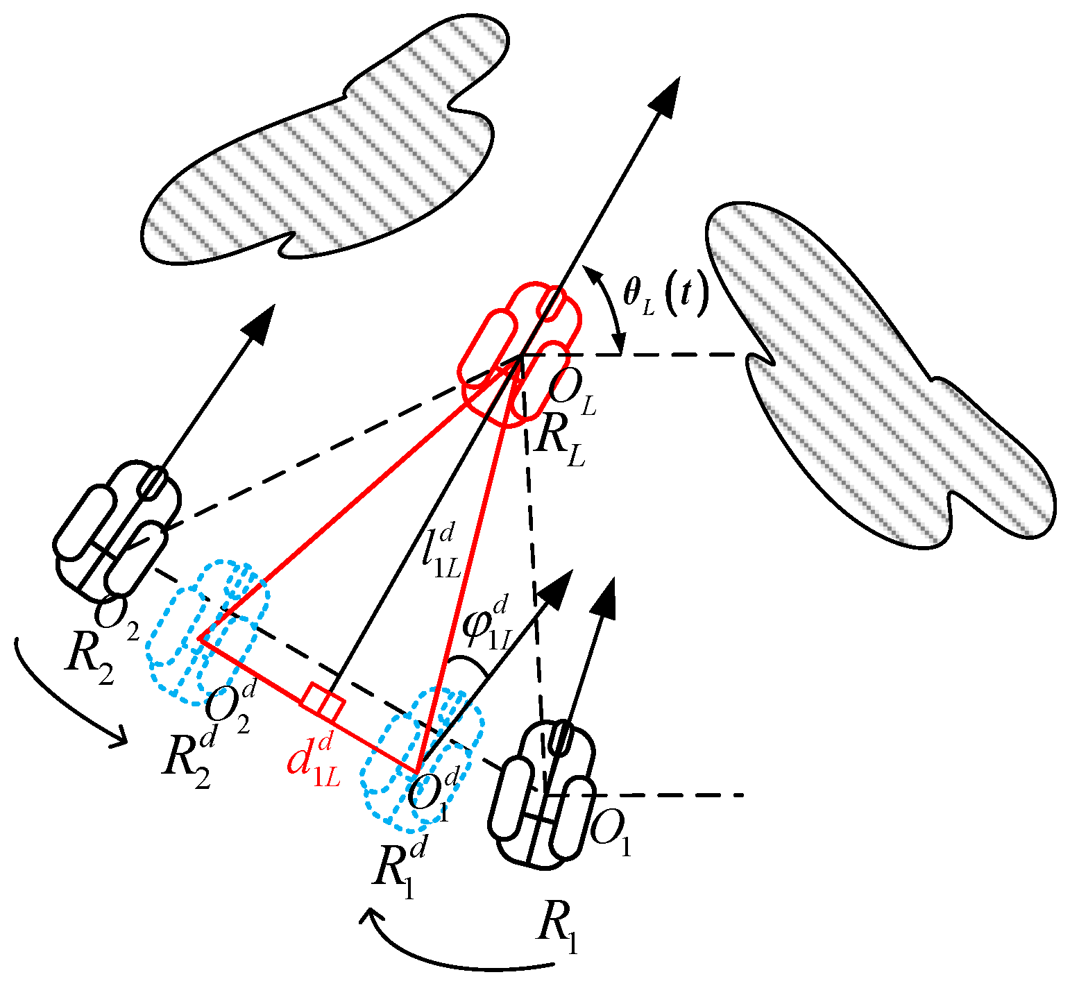
The follower robot maintains a constant distance from the leader robot, dynamically adjusts the relative angles between each following robot and the leader robot, and finally, follower robot and reach the points where the blue dashed line robot is located in Figure 5. The desired distance for the obstacle avoidance formation is the same as the desired distance for the predefined formation . The desired bearing angle is changed as in (21). The specific process is as follows.
To calculate the new desired bearing angle, define a distance , to be related to parameter and the radius of a robot’s protected shell , is as
The new bearing angle of the follower robot is calculated as
The next desired position of follower robot is denoted as and calculated as
The bearing angle for the next step is calculated as
3.2.4. Online Motion Planning for the Follower Robot with A Collision Problem
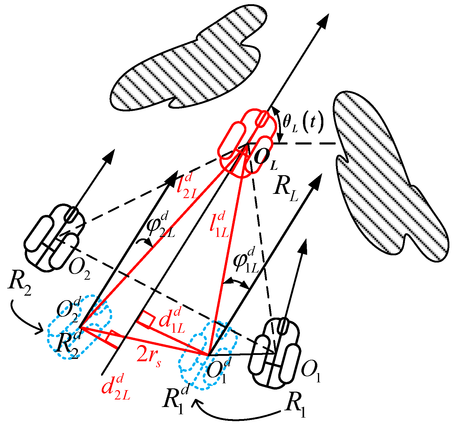
With the consideration of collision avoidance, the distance between two neighboring follower robots should be checked. If the distance between two follower robots is smaller than 2rs, to switch into the safe formation, the follower robot with low priority should change both desired distance and desired bearing angle with the leader robot. The desired position for the follower robot, with high priority, is calculated as (20)–(23), and the desired position for the follower robot with low priority is calculated as follows.
It is presumed that robot R2, with lower priority, calculates both new desired distance and desired bearing angle with leader robot to obtain the desired position in Figure 6. The length of is obtained by (20). The length of equals . The desired distance between the follower robot and the leader robot is calculated as
The new bearing angle of follower robot is calculated as
The next desired position of follower robot is denoted as calculated as
3.3. The Backstepping-Based Sliding Motion Controller
To achieve leader–follower formation through trajectory tracking control, it is necessary to ensure that the trajectory tracking error of the robot tends to zero at all times. In the leader–follower formation control system, each robot has the same inversion sliding mode variable structure motion controller during obstacle avoidance, which controls their respective pose errors to tend to zero. Thus, we combined the principle of sliding mode control and designed an inversion sliding mode variable structure motion controller for establishing a mobile robot formation based on a kinematics model.
According to the design principle of the sliding mode variable structure, the switching function of the tracking error is designed based on an inversion method, and then the control function of the formation tracking error is calculated, which is the motion controller of the robot.
To solve the motion controller of the ith robot, according to the sliding mode variable structure method, the first step is correctly designing the sliding mode switching function. The Lyapunov candidate function is designed based on the inversion method.
According to Equation (15), the differential equation of robot pose error is:
Assuming , calculating the first order partial derivative of the Lyapunov function , then
We get the Equation (22)
We make a detailed analysis about Equation (22) as follows:
- (1)
- if , then , , we can obtain ;
- (2)
- if , then , , we can obtain ;
- (3)
- if , then , , we can obtain ;
In summary, it can be concluded that no matter what value of is taken, can be obtained. Therefore, according to the definition of Lyapunov stability, as long as converges to zero and converges to , the state of the following robot in a multi mobile robot system converges to zero. Therefore, the sliding mode switching function of the robot’s motion controller can be designed as follows:
The discontinuous switching characteristics of the sliding mode control make the sliding mode motion prone to chattering on the sliding mode surface. For a sliding mode variable structure control system, the moving point will suffer from high-speed zigzag oscillation on the sliding surface trajectory, forcing the robot’s tracking error not to approach zero when the mobile robot is moving forward in a formation.
We utilize the double power reaching law to weaken the chattering phenomenon generated in the sliding mode variable structure formation control system. When the bounded disturbance exists, the double-power reaching rate can make the sliding mode and its first-order derivative converge to the steady-state error bound related to the upper bound within a limited time, thereby effectively weakening chattering. Therefore, our strategy affords fast convergence speed and second-order sliding mode after convergence, reducing the chattering of the trajectory tracking error.
Specifically, we set the double power-reaching rate as follows:
where . Si is the sliding mode variable selected in the sliding mode variable structure control design, representing the error variable between the robot’s ideal and the actual poses while moving forward during the trajectory tracking of the multi-mobile robot formation.
To reduce chattering, we employed a continuous function rather than a sign function:
By combining Equations (21)–(25), we obtained the following:
By transforming Equation (26), the speed and deceleration control quantities of the robots in the multi-robot leader-following formation tracking control system are:
where .
For the multi-robot formation generation and maintenance problems, when the trajectory of the leader robot is known, the motion controller drives the follower robot to track its ideal pose all the time, completing the formation and maintaining the formation operation. The leader robot uses the developed controller to track the virtual sub-target point in real time, and the follower robot uses our controller to adjust the formation dynamically.
4. Experiments
We conducted several simulation experiments under various obstacle distributions and number of following robots to verify the effectiveness of the proposed formation planning and obstacle avoidance strategy. The simulations involve five groups.
The initial position coordinates of the robot leader, follower 1, follower 2, follower 3, and follower 4 are (0, 9 m), (0, 8 m), (0, 10 m), (0, 11 m), and (0, 7 m). The initial linear velocity of the leader robot , angular velocity , , and . The controller simulation parameters are:
In the following experiments, the triangular formation refers to the expected triangular formation formed by the leader, follower 1, and follower 2, and the pentagonal formation refers to the expected pentagonal formation formed by the leader and follower 1, follower 2, follower 3, and follower 4.
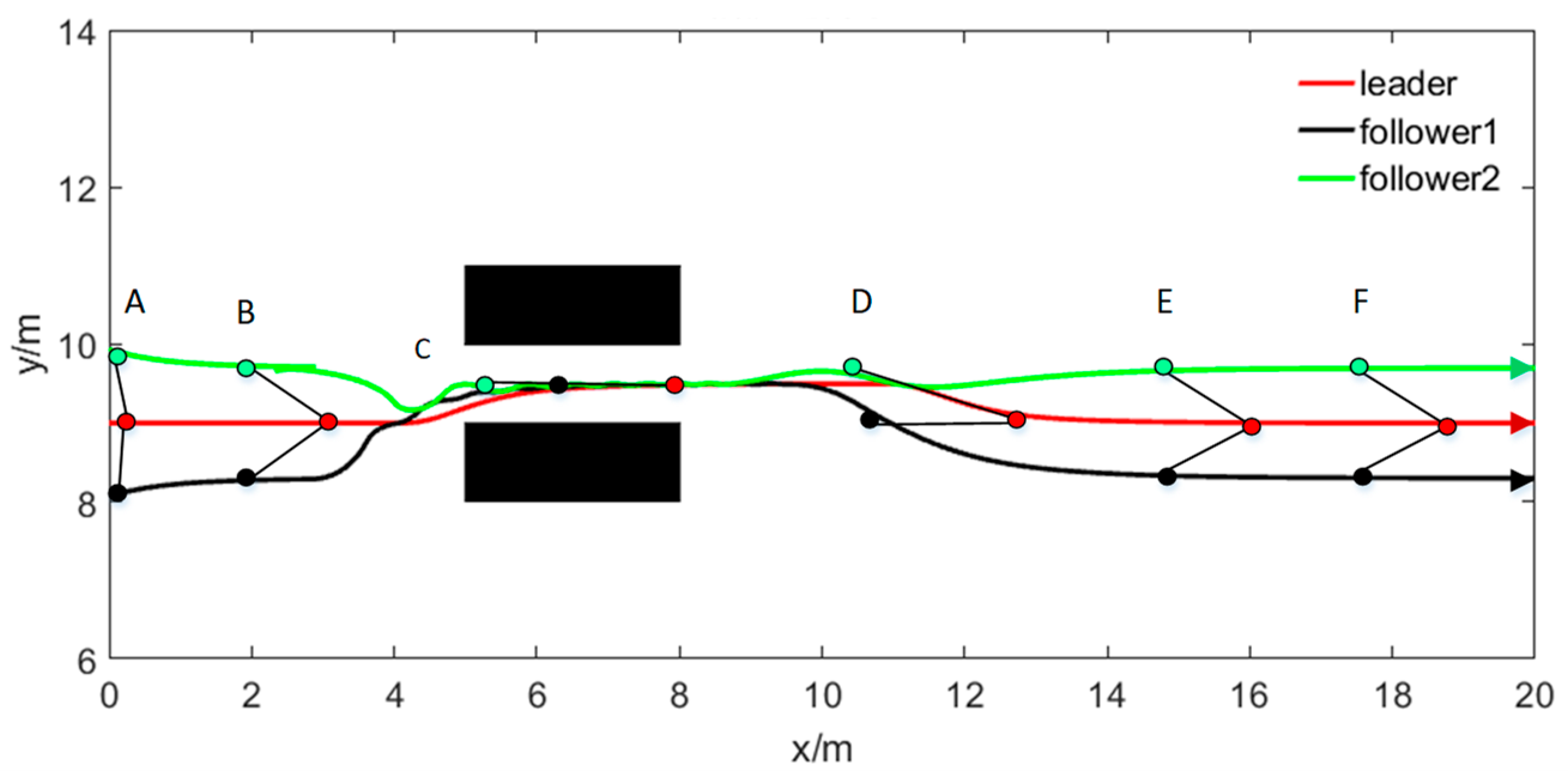
4.1. Online Obstacle Avoidance of Triangular Formation under the Condition of a Single Obstacle
Considering a triangular formation formed by the leader, follower 1, and follower 2 for a single obstacle scenario, the expected formation is = 1.4 m, = 1.4 m, = , =.
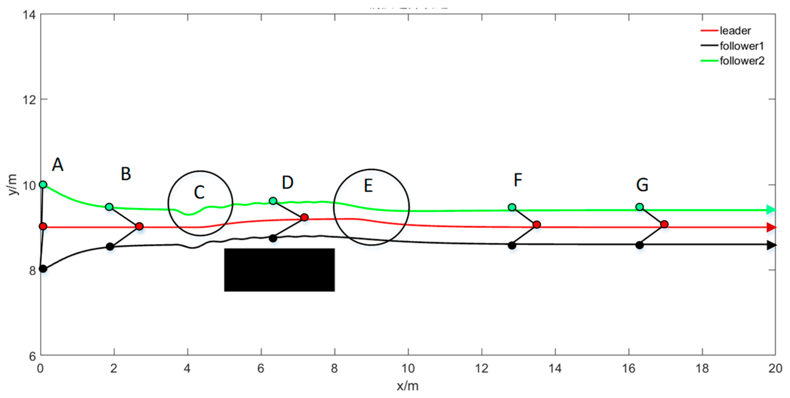
The motion trajectory of the online obstacle avoidance formation is illustrated in Figure 7. Before the formation encounters an obstacle, the entire formation forms a preset desired formation from the initially disordered state (A to B) and continues to move forward in this formation. The formation enters the online collaborative obstacle avoidance mode when the leader robot detects an obstacle ahead of it. Specifically, first, the condition of a single obstacle is judged based on the sensor information, and the leader robot leads the entire formation to bypass the obstacle (C–D–E). When the entire formation has bypassed the obstacle, the formation will continue to move forward after returning to the desired formation (F and G).
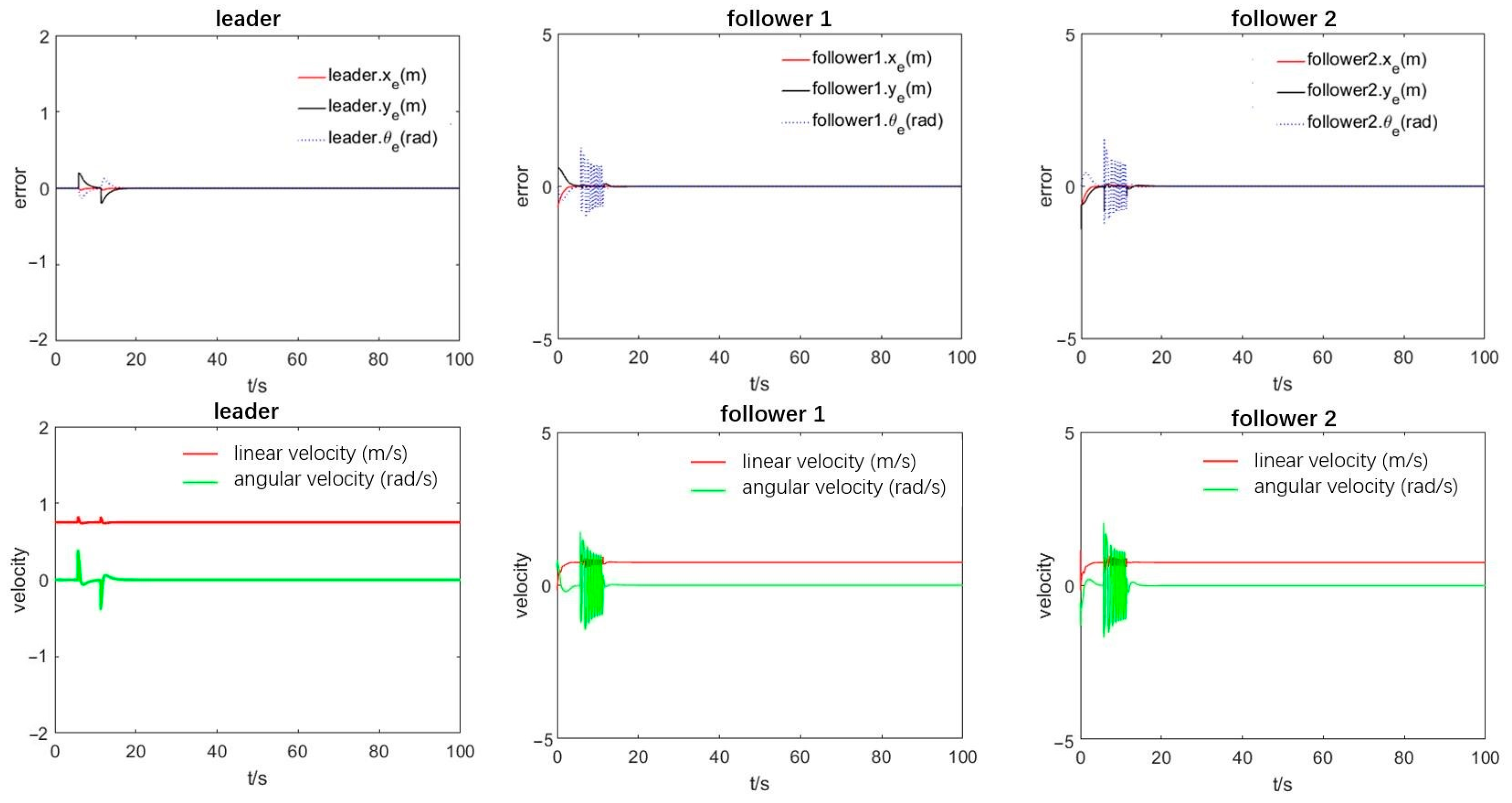
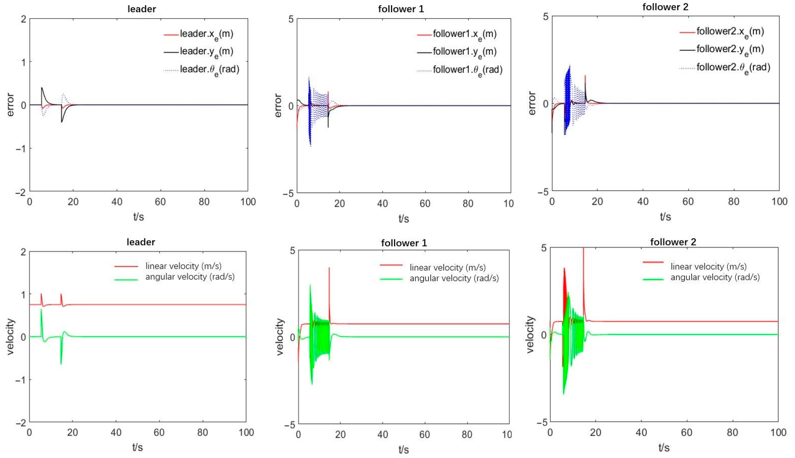
From the speed and position deviation curves of the leader robot presented in Figure 8, we conclude that when the leader robot initially encounters an obstacle, the speed and position will fluctuate significantly due to the leader robot’s real-time obstacle position during the obstacle avoidance process. The leader’s speed and angle are adjusted from the speed and error curves of the following robots in the formation, revealing that when encountering obstacles, each following robot judges if collision avoidance is required under the guidance of the leader robot. Accordingly, the following robots avoid obstacles based on the obstacle avoidance rules. Specifically, the relative azimuth of the leader robot changes to plan the obstacle avoidance path and drives the leader to track the obstacle avoidance path points planned at each moment through the controller. Figure 6 highlights that there will be a jitter during the tracking process, imposing the angular velocity direction to the jitter for a long time and increasing the angular velocity error. Ultimately, the leader’s speed and position gradually adjust according to the path planning to pass the obstacle area, which, once passed, the leader returns to the original formation in a short time after passing the obstacle area. The simulation results show that the proposed leader-following obstacle avoidance strategy is effective for a formation passing a single obstacle.
4.2. Triangular Formation Online Obstacle Avoidance under the Condition of Double Obstacles
In the double obstacle scenario, the triangle formation is considered under the parameters = 1.4 m, = 1.4 m, = , =. To verify the algorithm’s generalization ability and based on the obstacle distribution distance and the different formation shapes after adjusting the formation to avoid obstacles, three groups of double obstacles with distribution distances of 0.8 m, 1.0 m, and 2.0 m were selected.
Figure 9 depicts the trajectory of an online obstacle avoidance formation. During the obstacle-free stage, the formation is formed from the initial state, preserving the desired formation while moving toward the target point (A to B). When the formation arrives at a certain position and the leader robot detects an obstacle along the path, the leader will adjust the local trajectory for online obstacle avoidance, and at the same time, the follower robots conduct a collision avoidance judgment. The priority model determines that the follower 1 robot moves first, then the follower 1 robot keeps the distance from the leader robot unchanged, adjusts the relative angle to the leader robot, and avoids obstacles. Following this, follower 2 adjusts the relative distance and angle with the leader robot to avoid obstacles (B to C). Finally, the entire formation is led by the leader robot to obtain a new formation, and the robots will bypass the obstacle in a newly formed formation (C to D). When the entire formation has bypassed the obstacle, the formation will start to change (D), the robots will acquire the initial formation, and then move forward (E and F).
In the simulation results, Figure 10 presents the position error curves and control input of the leading and the following robots during the obstacle avoidance process. From the error diagram of the leader robot, it is evident that its relative distance error and motion direction error gradually decrease and finally converge to zero, demon-strating the successful tracking of the virtual sub-target. The error diagram of each follower robot shows that the robot’s error oscillation and speed change during the ob-stacle avoidance process are caused due to the various obstacle avoidance planning methods. For example, after about 10 s, each follower robot starts to avoid obstacles, and according to the priority, the follower 1 robot adjusts the angle with the leader ro-bot, presenting a longer angular oscillation than the follower 2 robot. However, obsta-cles can still be crossed. After the obstacle avoidance process completes, the error fi-nally converges to zero within a limited time, and the entire formation returns to the initial formation, verifying our method’s effectiveness.
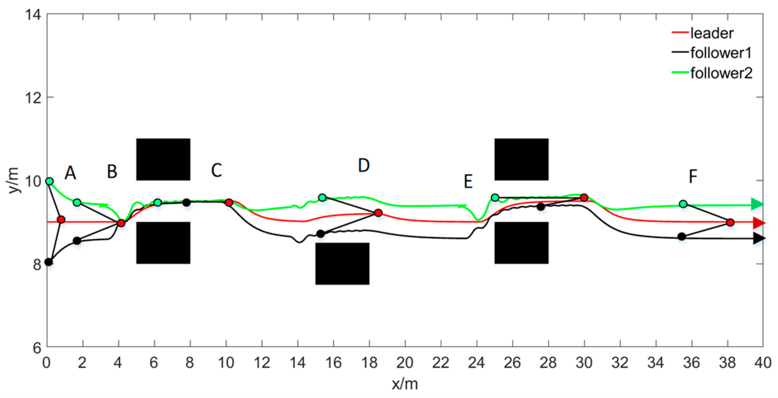
4.3. Triangular Online Obstacle Avoidance Formation under Mixed Obstacles
The simulation experiment was conducted using multiple obstacles in an unknown environment, involving three groups of obstacles: two considered double obstacles and one a single obstacle. The arrangement sequence is that the first double obstacle width is , the second is a single obstacle, and a third is a double obstacle with a width of . The expected formation parameters are , , = , = .
Figure 11 illustrates the online formation obstacle avoidance formation, where, in the obstacle-free stage, the entire formation moves from the initial state to the formation and maintains the initial formation toward the target point (A to B).
When the formation moves to a certain position, the leader robot detects the first obstacle on the path, determines the obstacle type, and adopts the corresponding obstacle avoidance planning method to conduct online obstacle avoidance planning. At the same time, the following robots within the formation apply the coordinated obstacle avoidance and collision avoidance rules. The follower robots avoid collisions after balancing the initial formation and obstacle width constraints. Therefore, according to the priority strategy, the robots independently conduct obstacle and collision avoidance planning and, finally, take the newly formed formation, which crosses the first obstacle (B to C).
After the formation leaves the obstacle avoidance area, it moves toward the target point and simultaneously begins to restore the initial formation. During their motion, the leader robot continues to detect the environment. At t = 20 s, it detects the second obstacle. At this time, the leader robot identifies the obstacle type before it and adopts the obstacle avoidance plan for a single obstacle. The formation starts to enter the online collaborative obstacle avoidance process. After the initial formation and the safe obstacle avoidance distance are balanced, the entire formation autonomously performs obstacle planning, and the formation finally bypasses the second obstacle (D).
When the last robot in the formation leaves the obstacle avoidance area, the formation leaves the obstacle avoidance track and continues to move toward the target point. At the same time, it begins to restore the initial formation. The leader robot continues to detect the environment. At about t = 32 s, it detects the third obstacle area. The leader robot identifies the type of obstacles ahead of it according to the environment modeling strategy and adopts the corresponding path planning. At the same time, the formation starts to enter the online collaborative obstacle and collision avoidance mode. Based on the obstacle width and according to the priority strategy, each robot independently conducts obstacle avoidance and collision avoidance planning, and the formation finally passes through the third obstacle area in a new formation (E). When the last robot in the formation leaves the obstacle-avoidance area, the formation leaves the obstacle-avoidance track, continues moving toward the target point, and restores the initial formation (F).
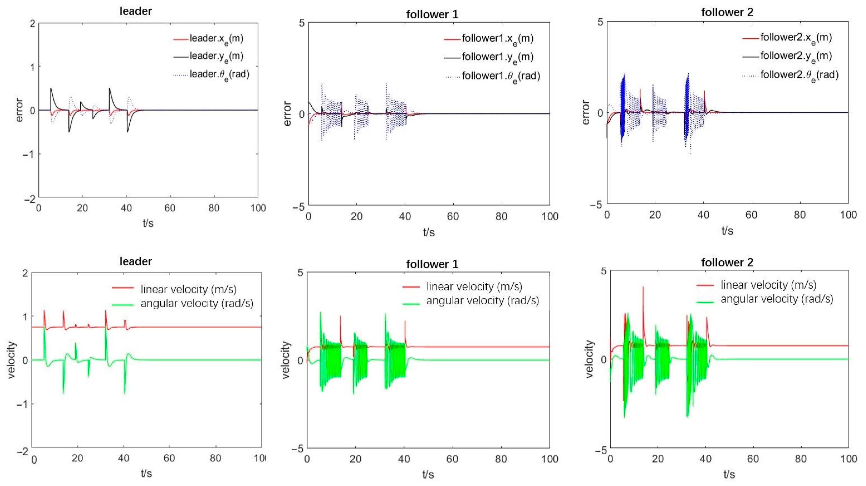
Figure 12 depicts the leading and follower robots’ position error curves and control input during the obstacle avoidance process. The leader’s error graph reveals that the leader robot’s relative distance error and the relative motion direction error gradually decrease and finally converge to zero, achieving successful pose tracking. From the error diagrams of each follower robot, it can be seen that the follower robot is always adjusting the direction of the leader robot during the obstacle avoidance process, and there are error oscillations and sudden speed changes. Moreover, each follower robot successfully passes through each obstacle. After obstacle avoidance, the error finally converges to zero within a limited time, and the entire formation restores its original formation, verifying the validity of the proposed paper to a certain extent.
4.4. Experiments of Leader–Follower Formation Planning
To validate the effectiveness and robustness of our multi-robot formation platform, we conducted a leader–follower formation experiment in the lab (Figure 12). The mobile robot hardware platform includes STM32F407 microprocessor, angular acceleration MPU6050, wireless communication unit ESP8266, and mobile beacons. The Marvelmind Indoor positioning system was used to obtain the positions of the robots. The experiment setup for leader–follower formation control is as follows:
(1) The whole robots connect to the same Wi-Fi network.
(2) TCP-Server1 and TCP-Server2 are created by the leader robot and the host computer, respectively.
(3) Each follower robot as a TCP-Client connects to TCP-Server1 and TCP-Server2. The posture of the leader robot is transmitted to each follower by the Wi-Fi network from TCP-Server1 to each TCP client. Meanwhile, the postures information, including the follower’s posture and the leader’s posture, is transmitted to the host computer from each TCP client to TCP-Server2.
(4) For crossing and avoiding obstacles, the leader robot calculates its posture to avoid obstacles using Virtual Sub-Goal according to Equations (5)–(17). The follower robots check the distance between the neighbor, and if it is without collision avoidance, they calculate the new safe desired bearing angle with the leader robot according to Equations (20)–(23). If a collision occurs, the follower robot with high priority only calculates the new desired bearing angle to obtain a safe posture according to Equations (20)–(23), and the follower robot with lower priority calculates the new desired distance and new desired bearing angle to obtain a safe posture according to Equations (24)–(27).
(5) During the process of controller calculation, the follower robots obtain the control inputs, which is the follower robots’ line velocity and angular velocity according to Equation (28). At last, they move into the desired formation to cross and avoid obstacles.
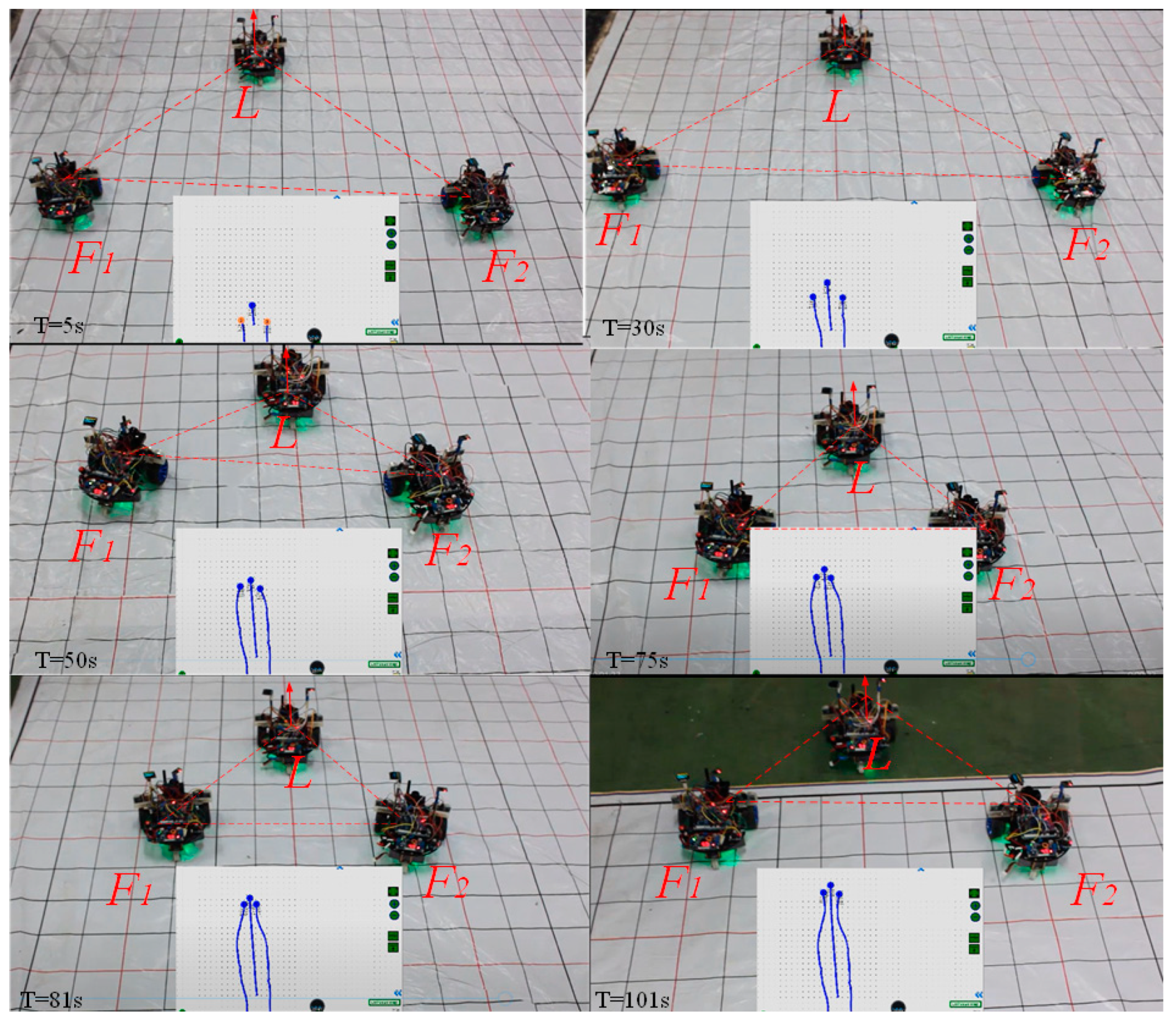
In this experiment, the three robots form a triangular formation from a random state and maintain formation operation along a straight track under external interference. The initial parameters for the leader robot are coordinates (3.24 m, 2.29 m), motion direction leader. θ=π/2, linear velocity , and angular velocity . Regarding the follower robots: follower 1 coordinates (2.61 m, 1.96 m), direction follower1.θ = π/2, and for follower 2 coordinates (3.83 m, 2.10 m), and direction follower2.θ = π/2. The three robots complete the equilateral triangle formation during the operation l = 0.3 m.
From the real-time dynamic display window at the bottom of the figure, it can be seen that multiple mobile robots can generate an equilateral triangle with the expected formation l = 0.3 m from the initially disordered state and preserve it while moving forward. During the running process, the robots can complete the formation switching from l = 0.3 m to l = 0.6 m, which is about t = 50–80 s, and the robots do not fall behind during this process. The video frames presented in Figure 13 highlight that when the formation changes, the angular and linear velocities of the follower 1 and follower 2 robots significantly jitter. After the shape transformation is completed, the linear and angular velocities stabilize, and both follower robots still move at the same speed as the leader to achieve consistency. However, there will be delays, blind connections, and discontinuous movements during the robot communication process. Finally, both followers are adjusted in time through the motion controller to form a formation and keep the formation moving forward.
5. Conclusions
This paper proposes a leader–follower formation and online motion planning strategy. Specifically, we first developed the leader–follower setup’s kinematics model and then proposed a virtual sub-target-based obstacle avoidance method. The leader robot establishes a series of virtual transition sub-targets based on the obtained sensor information and the target point position. The motion planning is based on a changing formation strategy and a priority model. Considering the former, the leader robot adopts the formation adjustment strategy to dynamically adjust the relative distance or relative azimuth to the leader robot and to avoid obstacles. To solve the formation adjustment problem, we developed a priority model to determine the priority movement of the following robots. In the future, we will focus on formation motion planning in dynamic environments.
Author Contributions
Conceptualization, H.C. and T.Z.; methodology, H.C., W.M., X.L., Q.W. and Z.W.; software, H.C. and Z.W.; validation, H.C. and Z.W.; formal analysis, H.C.; writing—original draft preparation, T.Z.; writing—review and editing, T.Z., H.C., X.L. and W.Z.; supervision, T.Z.; funding acquisition, X.L. All authors have read and agreed to the published version of the manuscript.
Funding
This work was funded in parts by National Natural Science Foundation of China (62003218), Stable Support Projects for Shenzhen Higher Education Institutions (20220717223051001), Shenzhen Overseas Talent Program (2021024555101050), University-Industry Cooperation Grant (2022010802011), and Education Center Industry-University Grant (2021JQR003).
Data Availability Statement
Data are available upon request.
Conflicts of Interest
The authors declare no conflict of interest.
References
- Ahmed, A.A.; Abdalla, T.Y.; Abed, A.A. Path planning of mobile robot by using modified optimized potential field method. Int. J. Comput. Appl. 2015, 113, 6–10. [Google Scholar] [CrossRef] [Green Version]
- Arrichiello, F.; Chiaverini, S.; Indiveri, G.; Pedone, P. The null-space-based behavioral control for mobile robots with velocity actuator saturations. Int. J. Robot. Res. 2010, 29, 1317–1337. [Google Scholar] [CrossRef]
- Benzerrouk, A.; Adouane, L.; Martinet, P. Stable navigation in formation for a multi-robot system based on a constrained virtual structure. Robot. Auton. Syst. 2014, 62, 1806–1815. [Google Scholar] [CrossRef] [Green Version]
- Cetin, M. The effect of urban planning on urban formations determining bioclimatic comfort area’s effect using satellitia imagines on air quality: A case study of Bursa city. Air Qual. Atmos. Health 2019, 12, 1237–1249. [Google Scholar] [CrossRef]
- Cruz-Morales, R.D.; Velasco-Villa, M.; Castro-Linares, R.; Palacios-Hernandez, E.R. Leader-follower formation for non- holonomic mobile robots: Discrete-time approach. Int. J. Adv. Robot. Syst. 2016, 13, 46. [Google Scholar] [CrossRef] [Green Version]
- Darmanin, R.N.; Bugeja, M.K. A review on multi-robot systems categorised by application domain. In Proceedings of the 2017 25th Mediterranean Conference on Control and Automation (MED), Valletta, Malta, 3–6 July 2017; IEEE: New York, NY, USA, 2017; pp. 701–706. [Google Scholar]
- Deghat, M.; Anderson, B.D.O.; Lin, Z. Combined flocking and distance-based shape control of multi-agent formations. IEEE Trans. Autom. Control 2015, 61, 1824–1837. [Google Scholar] [CrossRef] [Green Version]
- Di Caro, G.A.; Yousaf, A.W.Z. Multi-robot informative path planning using a leader-follower architecture. In Proceedings of the 2021 IEEE International Conference on Robotics and Automation (ICRA), Xi’an, China, 30 May 2021–5 June 2021; IEEE: New York, NY, USA; pp. 10045–10051. [Google Scholar]
- Fahimi, F.; Rineesh, S.V.S.; Nataraj, C. Formation controllers for underactuated surface vessels and zero dynamics stability. Control Intell. Syst. 2008, 36, 277–287. [Google Scholar]
- Guo, M.; Zavlanos, M.M.; Dimarogonas, D.V. Controlling the relative agent motion in multi-agent formation stabilization. IEEE Trans. Autom. Control 2013, 59, 820–826. [Google Scholar] [CrossRef]
- Li, F.; Ding, Y.; Hao, K. A dynamic leader- follower strategy for multi-robot systems. In Proceedings of the 2015 IEEE International Conference on Systems, Man, and Cybernetics, Hong Kong, China, 9–12 October 2015; pp. 298–303. [Google Scholar]
- Sun, X.; Wang, G.; Fan, Y.; Mu, D.; Qiu, B. A Formation collision avoidance system for unmanned surface vehicles with leader-follower structure. IEEE Access 2019, 7, 24691–24702. [Google Scholar] [CrossRef]
- Liu, X.; Ge, S.S.; Goh, C.-H. Formation potential field for trajectory tracking control of multi-agents in constrained space. Int. J. Control 2016, 90, 2137–2151. [Google Scholar] [CrossRef]
- Lu, Y.; Guo, Y.; Dong, Z. Multiagent flocking with formation in a constrained environment. J. Control Theory Appl. 2010, 8, 151–159. [Google Scholar] [CrossRef]
- Rajvanshi, A.; Islam, S.; Majid, H.; Atawi, I.; Biglerbegian, M.; Mahmud, S. An efficient potential-function based path-planning algorithm for mobile robots in dynamic environments with moving targets. Br. J. Appl. Sci. Technol. 2015, 9, 534–550. [Google Scholar] [CrossRef]
Figure 1.
Geometric structure model of the mobile robot driven by two rear wheels.

Figure 2.
Kinematics model of leader–follower formation.

Figure 3.
Schematic diagram of the leader robot’s online obstacle avoidance planning for a single obstacle.
Figure 3.
Schematic diagram of the leader robot’s online obstacle avoidance planning for a single obstacle.

Figure 4.
Schematic diagram of the online motion planning of the leader robot for a double obstacle scenario.
Figure 4.
Schematic diagram of the online motion planning of the leader robot for a double obstacle scenario.

Figure 5.
Schematic diagram of the online motion planning for the follower robot without the collision problem scenario.
Figure 5.
Schematic diagram of the online motion planning for the follower robot without the collision problem scenario.

Figure 6.
Schematic diagram of the online motion planning for the follower robot with collision problem scenario.
Figure 6.
Schematic diagram of the online motion planning for the follower robot with collision problem scenario.

Figure 7.
Online triangular formation obstacle avoidance trajectory for a single obstacle scenario.

Figure 8.
Trajectory error vs. control input variation curve.

Figure 9.
Online triangular formation obstacle avoidance trajectory for the double obstacles scenario.
Figure 9.
Online triangular formation obstacle avoidance trajectory for the double obstacles scenario.

Figure 10.
Trajectory error vs. control input variation curve under the condition of double obstacles.
Figure 10.
Trajectory error vs. control input variation curve under the condition of double obstacles.

Figure 11.
Triangular online obstacle avoidance trajectories under mixed-obstacle conditions.

Figure 12.
Trajectory error vs. control input variation curve under mixed obstacles.

Figure 13.
Snapshots of the triangle formation (https://youtu.be/mflFBvPQiQQ (accessed on 23 July 2023)).
Figure 13.
Snapshots of the triangle formation (https://youtu.be/mflFBvPQiQQ (accessed on 23 July 2023)).

Disclaimer/Publisher’s Note: The statements, opinions and data contained in all publications are solely those of the individual author(s) and contributor(s) and not of MDPI and/or the editor(s). MDPI and/or the editor(s) disclaim responsibility for any injury to people or property resulting from any ideas, methods, instructions or products referred to in the content. |
© 2023 by the authors. Licensee MDPI, Basel, Switzerland. This article is an open access article distributed under the terms and conditions of the Creative Commons Attribution (CC BY) license (https://creativecommons.org/licenses/by/4.0/).
Share and Cite
MDPI and ACS Style
Chen, H.; Wang, Z.; Liu, X.; Ma, W.; Wang, Q.; Zhang, W.; Zhang, T. A Hybrid Motion Planning Algorithm for Multi-Mobile Robot Formation Planning. Robotics 2023, 12, 112. https://doi.org/10.3390/robotics12040112
AMA Style
Chen H, Wang Z, Liu X, Ma W, Wang Q, Zhang W, Zhang T. A Hybrid Motion Planning Algorithm for Multi-Mobile Robot Formation Planning. Robotics. 2023; 12(4):112. https://doi.org/10.3390/robotics12040112
Chicago/Turabian StyleChen, Haojie, Zifan Wang, Xiaoxu Liu, Wenke Ma, Qiang Wang, Wenjun Zhang, and Tan Zhang. 2023. "A Hybrid Motion Planning Algorithm for Multi-Mobile Robot Formation Planning" Robotics 12, no. 4: 112. https://doi.org/10.3390/robotics12040112
Note that from the first issue of 2016, this journal uses article numbers instead of page numbers. See further details here.