
Trajectory Control of An Articulated Robot Based on Direct Reinforcement Learning
1
Department of Mechanical Engineering, National Taiwan University, No. 1, Sec. 4, Roosevelt Rd., Taipei 106216, Taiwan
2
Department of Mechanical Engineering, National Taiwan University of Science and Technology, No. 43, Sec. 4, Taipei 106335, Taiwan
*
Author to whom correspondence should be addressed.
Robotics 2022, 11(5), 116; https://doi.org/10.3390/robotics11050116
Submission received: 6 September 2022
/
Revised: 13 October 2022
/
Accepted: 17 October 2022
/
Published: 20 October 2022
(This article belongs to the Section Industrial Robots and Automation)
Abstract
:Reinforcement Learning (RL) is gaining much research attention because it allows the system to learn from interacting with the environment. Yet, with all these successful applications, the application of RL in direct joint torque control without the help of an underlining dynamic model is not reported in the literature. This study presents a split network structure that enables successful training of RL to learn the direct torque control for trajectory following a six-axis articulated robot without prior knowledge of the dynamic robot model. The training took a very long time to converge. However, we were able to show the successful control of four different trajectories without needing an accurate dynamics model and complex inverse kinematics computation. To show the RL-based control’s effectiveness, we also compare the RL control with the Model Predictive Control (MPC), another popular trajectory control method. Our results show that while the MPC achieves smoother and more accurate control, it does not automatically treat the singularity. In addition, it requires complex inverse dynamics calculations. On the other hand, the RL controller instinctively avoided the violent action around the singularities.
1. Introduction
Reinforcement Learning allows the system to learn by interacting with the environment. There is no need for a large number of labeled samples, and the system learns as it accumulates experience. Since its introduction, RL has shown great potential in many applications.
This study addresses the direct application of Reinforcement Learning (RL) to the joint force control of an articulated robot to follow pre-specified trajectories. The RL controller uses a neural network to compute the required joint torque. It requires no knowledge of an underlying dynamic robot model and needs no complex inverse kinematics calculation. From the application point of view, a neural network-based robot arm controller is desirable. However, very few available RL robot control examples have addressed the direct torque control of articulated robots. Searching through the literature, one finds that most available results dealt only with the kinematic trajectory planning and left the torque control problem to the controller that came with the robot. Many related results have based their control on model-based inverse dynamic cancellation and used RL to learn the control parameters [1,2]. The others that did address direct joint torque were for SCARA robots with only two links [2,3]. Considering how humans learn to control their limbs, it is still desirable to know if one can train the robot arm the way we train ourselves to use our arm.
Learning control has been around for a long time. In 1995, Nuttin and Van Brussel proposed a learning controller to increase the insertion speed in consecutive peg-into-hole operations; the learning controller could perform the same without increasing the contact force level [4]. In 1997, Schaal examined the types of learning problems that benefit from demonstration [5]. He compared the performance of various learning algorithms on an anthropomorphic robotic arm. In 2006, Peters and Schaal demonstrated the efficiency of Reinforcement Learning in teaching a SARCOS Master Arm to hit a baseball [6]. In 2007, he also performed the Reinforcement Learning approach on the anthropomorphic robotic arm simulation in operational space control [7]. In 2010, Kober et al. explained the technique of learning mappings from circumstances to meta-parameters by using Reinforcement Learning. He showed two robot movement applications: throwing darts and table tennis hitting [8]. In 2016, Gu et al. showed that a Deep Reinforcement Learning algorithm based on the off-policy training of Deep Q-Functions could scale to complex 3D manipulation tasks for a robot [9]. In 2017, Liu et al. proposed an RL learning control for the robotic insertion task [10]. In 2018, Luo et al. used Guided Policy Search in the peg-in-hole insertion in a deformable hole [1].
Many RL approaches are available. The Deep Deterministic Policy Gradients (DDPG) is a state-of-the-art algorithm to simultaneously train the Deep Q Network and the Deep Policy Network. DDPG achieves good performance in continuous control problems by integrating the Deterministic Policy Gradient algorithm. From a comparative viewpoint, the difference between the Stochastic- and Deterministic Policy Gradient is that the Stochastic Policy Gradient integrates over both state and action spaces. In contrast, the Deterministic Policy Gradient only integrates over the state space. Consequently, the Deterministic Policy Gradient requires fewer samples than the Stochastic Policy Gradient, especially if the action space has few dimensions [11]. Survey papers at various stages of development on RL are already available. Kormushev provided a summary describing the RL application in the real world industry [12], and Wang et al. published a review of recent theoretical development [13]. There is also the convergence issue with the training algorithm. When Silver et al. first proposed the deterministic policy gradient (DPG) algorithm [11], they required a linear compatible function as the state-action value function. The DDPG proposed by Lillicrap et al. [14] uses a deep neural network (DNN) as a function approximator. The nonlinear approximator introduces a risk of trapping in the local optimal. Many literature results have shown that the main issue is the compatibility between the actor and critic networks. To avoid this situation, DDPG introduces the noisy state-action value function. Many research efforts have been devoted to exploring ways to improve convergence [15,16,17,18,19,20,21,22]. There are also alternative approaches to DDPG for continuous-time reinforcement learning. Ghavamzadeh and Mahadevan [23] developed a generalization of the MAXQ for continuous-time semi-Markov decision processes. Tiganj et al. [24] developed a logarithmically-compressed time scale model for the future to establish a scale-invariant timeline to overcome the discretization problem. Research by Jiao and Oh [25] proposed using separate threads to execute the “behavior” and the “update policy.” In this research, we adopted the method proposed by [14] to add noise to the actor policy to ensure value function compatibility.
This study used a HIWIN RA605 robotic arm for the target experiment. We defined the simulation’s target trajectory, reward function, policy, and actor-critic network structures. After many trials, it became clear that the direct application of RL to multi-link articulated robot trajectory control without an underlining model is more complicated than one expects. A recent study directly applied the deep learning controller to emulate the inverse dynamics action [26]. They handled the nonlinear behavior by applying the learning control on the separate axis with all the other axes fixed. However, they still used model-based supervised learning. In addition, their effort to train all the axes can be too great for practical implementation. Instead, our study based the training on the trajectory without needing a dynamic model. One can therefore train the RL network along a specific path. We describe the proposed network structure and the result of the training.
This study also compared the control with the Model Predictive Control (MPC), another popular control method, to demonstrate the control effectiveness. MPC based the design on a system model. Instead of conventional feedback, it determines the control action by optimizing a performance index over a finite time horizon [27]. Many previous researchers have proposed different MPC methods. In 2014, Nikdel designed an MPC controller to control a single-degree-of-freedom shape memory alloy (SMA) actuated rotary robotic arm to track the desired joint angle [28]. MPC discovered practices in dynamic and unpredictable environments such as chemical plants and oil refineries [29], as well as power system balancing [30]. More recently, the MPC has also begun to find applications in the control of autonomous vehicles [31] and robotic trajectory control [32,33,34]. In 2016, Best et al. applied MPC to robot joint control. The dynamic model-based control of a soft robot shows significant improvement over the regular controller [35]. In 2017, Lunni et al. applied a Nonlinear Model Predictive Controller (NMPC) to an aerial robotic arm for tracking desired 3D trajectories. They demonstrated online use of the NMPC controller with limited computational power [36]. In 2018, Guechi et al. proposed a combination of MPC and feedback linearization control for a two-link robotic arm [37,38]. In the same year, Car et al. applied an MPC-based position control to an unmanned aerial vehicle (UAV). The onboard computer running linear MPC-based position control communicates through a serial port with the low-level altitude controller [39].
This paper describes using RL to control a HIWIN RA605 robotic arm. The task is for the robot arm to follow a desired trajectory while maintaining a specific attitude for the end effector. We propose a split network structure that allows for the direct application of RL to robot trajectory control. We also compare the control performance to a Twin Delayed Deep Deterministic Policy Gradient (TD3) network and an MPC. The results show that the proposed RL structure can achieve articulated robot control without the help of an accurate robot model. The RL trajectory is oscillatory but instinctively avoids the singularity and requires no background model. The behavior is similar to a human holding out their hand. Although the TD3 controller still converges, it oscillates around a noticeable offset. The MPC is smooth but requires a system model and additional treatments to avoid singularities.
2. Theoretical Background
2.1. Deep Deterministic Policy Gradient (DDPG)
The popular DDPG was first used in this study to train the RL network. The standard reinforcement learning algorithm considers the problem of an agent interacting with an environment . The policy for the agent’s action at state is represented by a probability distribution , where represents the state space and represents the action space. Assuming that the actions can be parameterized with parameters ; the parameterized policy becomes which selects the action in state with parameters by interacting with the environment. At each time step , the agent receives a reward for its action, and the return from a state is defined by the sum of the discounted future reward . As a result, the expected return, or the value function, for the action becomes . The goal of the agent is to maximize the value function by updating and . To allow an iterative learning process, one can express the value function in a recursive form: . One can omit the inner expectation if one chooses a deterministic policy as , and reduces the value function to an expression that depends only on the environment such as . It is now possible to use an off-policy algorithm to learn with a greedy policy .
The standard RL algorithm is not directly applicable to continuous action space due to the need for optimization at every time step. DDPG thus resolves into an actor-critic model structure. The actor specifies the deterministic policy by mapping the states to a specific action. The critic then learns the value function using the Bellman equation. The policy gradient of the expected return can be expressed as:
The basic algorithm for DDPG is shown in Algorithm 1.
Algorithm 1: DDPG
- Initialize and arbitrarily, set and , iterate until they converge.
- For every episode:
- For every time step :
- Given a state , take action based on policy ;
- Obtain reward and the new state ;
- Store all the (,,,) into the buffer.
- Sample a batch of (,,,) from the buffer;
- Set the cost function ;
- Update the parameters of , which is , to minimize .
Set the value function:
Update the parameters of , which is , to maximize .
Update and , where is a factor between 0 and 1.
2.2. The Modified DDPG Method
As mentioned before, the algorithm in the previous subsection adopted the greedy policy to optimize for each time step and is unsuitable for applying to continuous-time robotic motion control. Therefore, modifying the algorithm into an applicable actor-critic algorithm is necessary.
In the DDPG algorithm, is used to represent the decision-making policy that determines the corresponding action in the state . The decision of the action by does not result directly from the information of the state and would require two steps to determine. Suppose there are five possible discrete actions, will first decide on the most probable action and use it as its decision. Nevertheless, due to the greedy selection, the final choice may not be the same as the action with the highest possibility.
In this paper, the action consists of six joint torques; there is an infinitely possible choice of actions because the torque is a continuous variable. As a result, the possibility of all activities being covered cannot be covered. Instead of using to determine the most probable action, the algorithm resolves to using to directly determine the action , which consists of the six joint torques, based on the states . The algorithm also added noise to the action to ensure value function compatibility.
The modified DDPG method (DDPG-1) algorithm is shown as Algorithm 2.
Algorithm 2: DDPG-1
- Initialize and arbitrarily, set and , iterate until converge;
- For every episode.
- For every time step :
- Given a state , take action based on ;
- Obtain reward and each new state ;
- Store all (,, , ) into the buffer.
- Sample a batch of (, , , ) from the buffer;
- Set the cost function.
Update the parameters of , which is to minimize .
Set the value function:
Update the parameters of , which is to maximize .
- Update and , where is a factor between 0 and 1.
Using the DDPG-1 method, one can consistently update the parameters of the critic and the policy consistently during training to obtain the optimized critic and policy . For each training step, the action selected is , where is the noise for value function compatibility. We also explored the TD3 algorithm, but it did not provide too much improvement.
2.3. The Differential Kinematics
The robotic control is slightly more complicated than the standard control systems. Unlike the regular control system that directly takes the control error for feedback, the control system needs to adequately translate the trajectory error in the task space into the various joint torques. In other words, there is a transformation of the measurement from the “task space” into the “joint space,” and the translation involves the differentiation of the Jacobian matrices, which, in turn, introduces Coriolis accelerations. The robotic control system will need to cancel or suppress this nonlinear effect. In a common end-following task, the position and attitude of the robot end-effector in the Cartesian coordinate system contain three position values (, , ) and three attitude angles (,,), for a total of six degrees of freedom. For an RA 605 robotic arm with six joints, the controller will need to perform the inverse kinematics and compute the nonlinear dynamic forces for cancellation and exercise the control. One of the goals of this research is to use a deep learning network for the inverse dynamic model and directly control the robotic arm.
3. The Reinforcement Learning Structure
The RL Network Structure
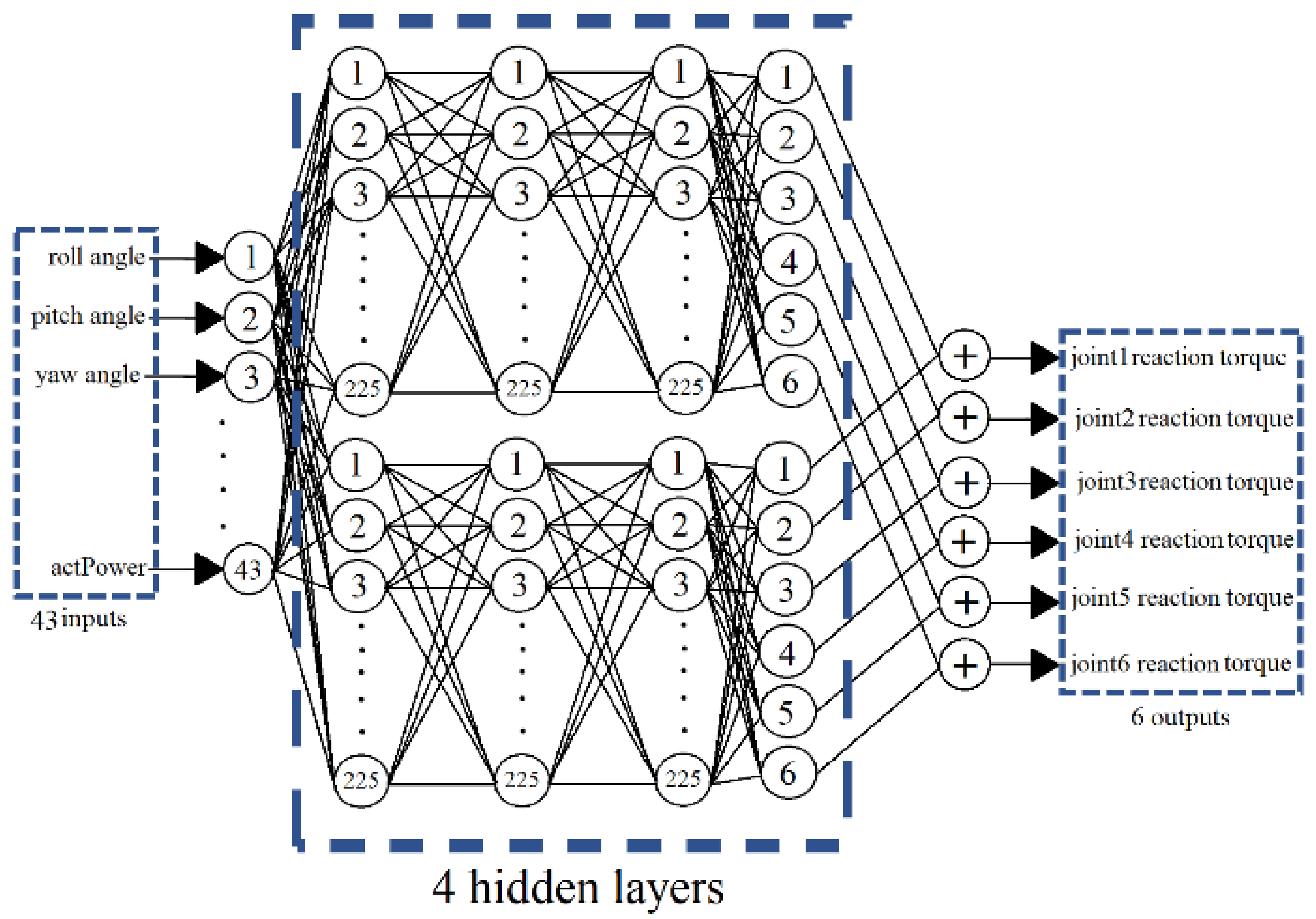
The following section will briefly describe the deep learning network setup. For the agent, we set 43 observed results as the inputs, including the roll angle , pitch angle , yaw angle , the roll angular velocity , pitch angular velocity , yaw angular velocity , the roll angular acceleration , pitch angular acceleration , and yaw angular acceleration . The measurements were made with respect to the end of the last joint relative to the reference coordinate. In addition, there are also three positions (), velocities (), and accelerations () of the endpoint of the robotic arm, also based on the reference coordinate. Furthermore, there are six joint angles (), six joints angular velocities (), six joints angular accelerations (), six joints torques (), and the total power of joints (). The outputs of the actor network are the six joint torques.
Although deep learning is a powerful tool, the computation effort involved in training the network can be too great for practical applications. Our initial attempt to help with the training was to separate the effect of the positioning error and the effect of the velocity error to prevent the conflicting demands from holding position and moving the arm. However, the learning behavior of the network was not predictable. After many attempts, we finally came up with a unique structure for the actor network. The actor network consists of two parallel networks, each with three 225-neuron fully connected hidden layers and a fully connected output layer, as shown in Figure 1.
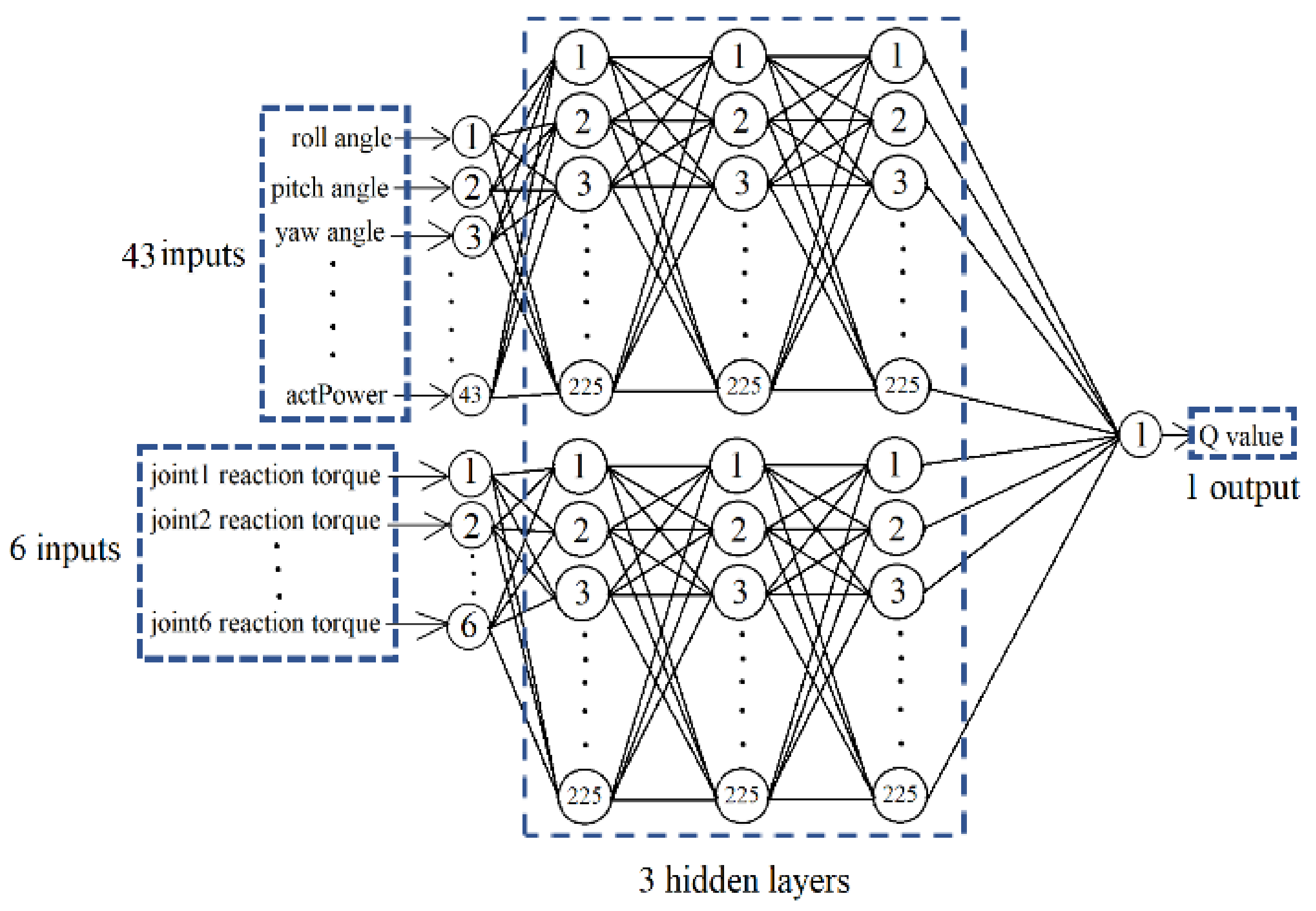
In addition, we also break down the critic network into two parts: one for observation and the other for the robot. The observation part of the network takes the 43 observed results as inputs, and the robot part takes the six joint torques as inputs. The two parts both consist of three fully connected hidden layers with 225 neurons. Their outputs combine to form the network Q value output, as shown in Figure 2.
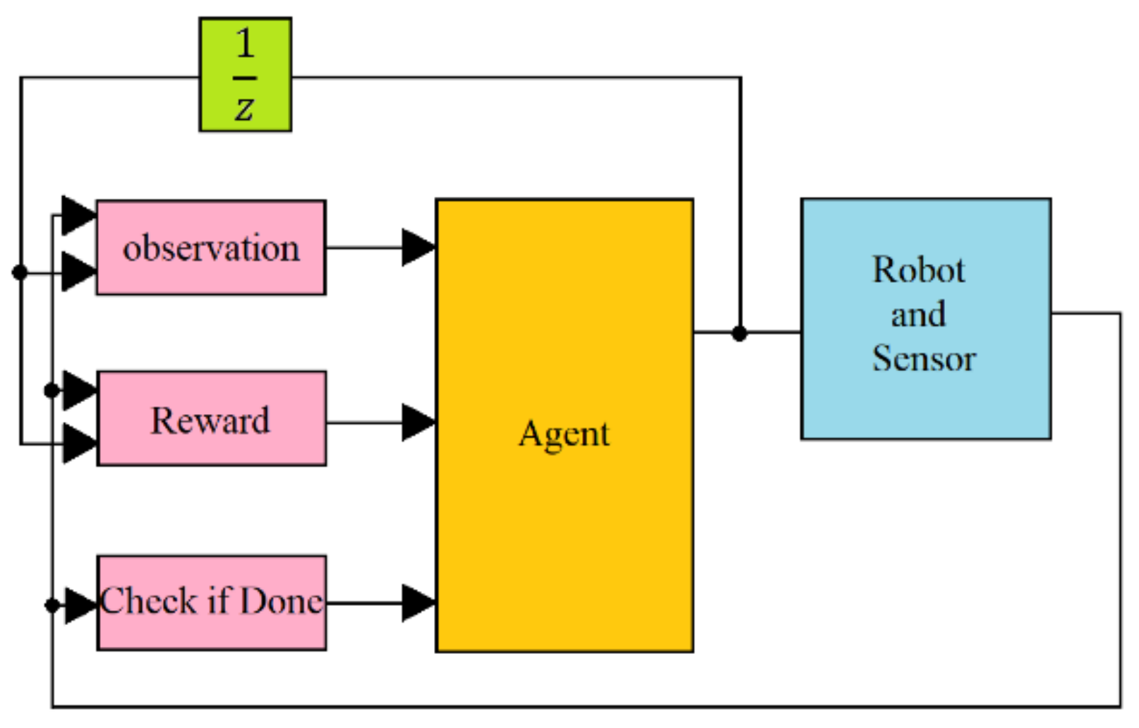
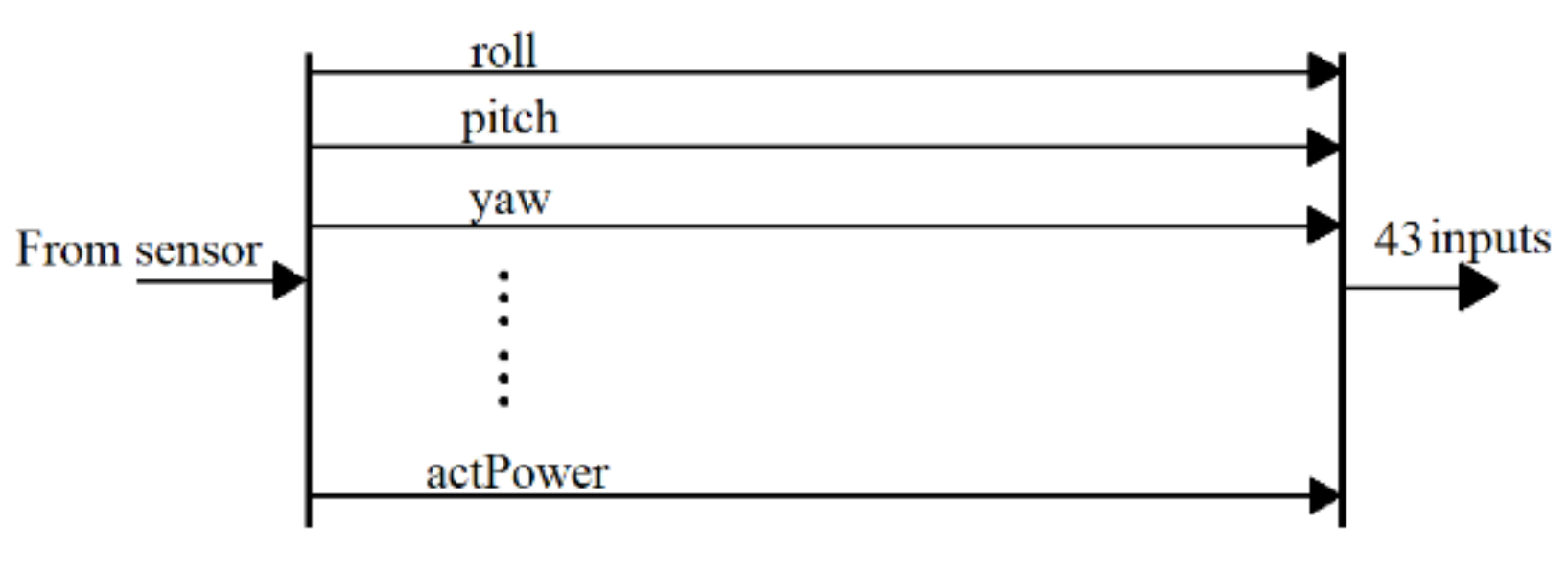
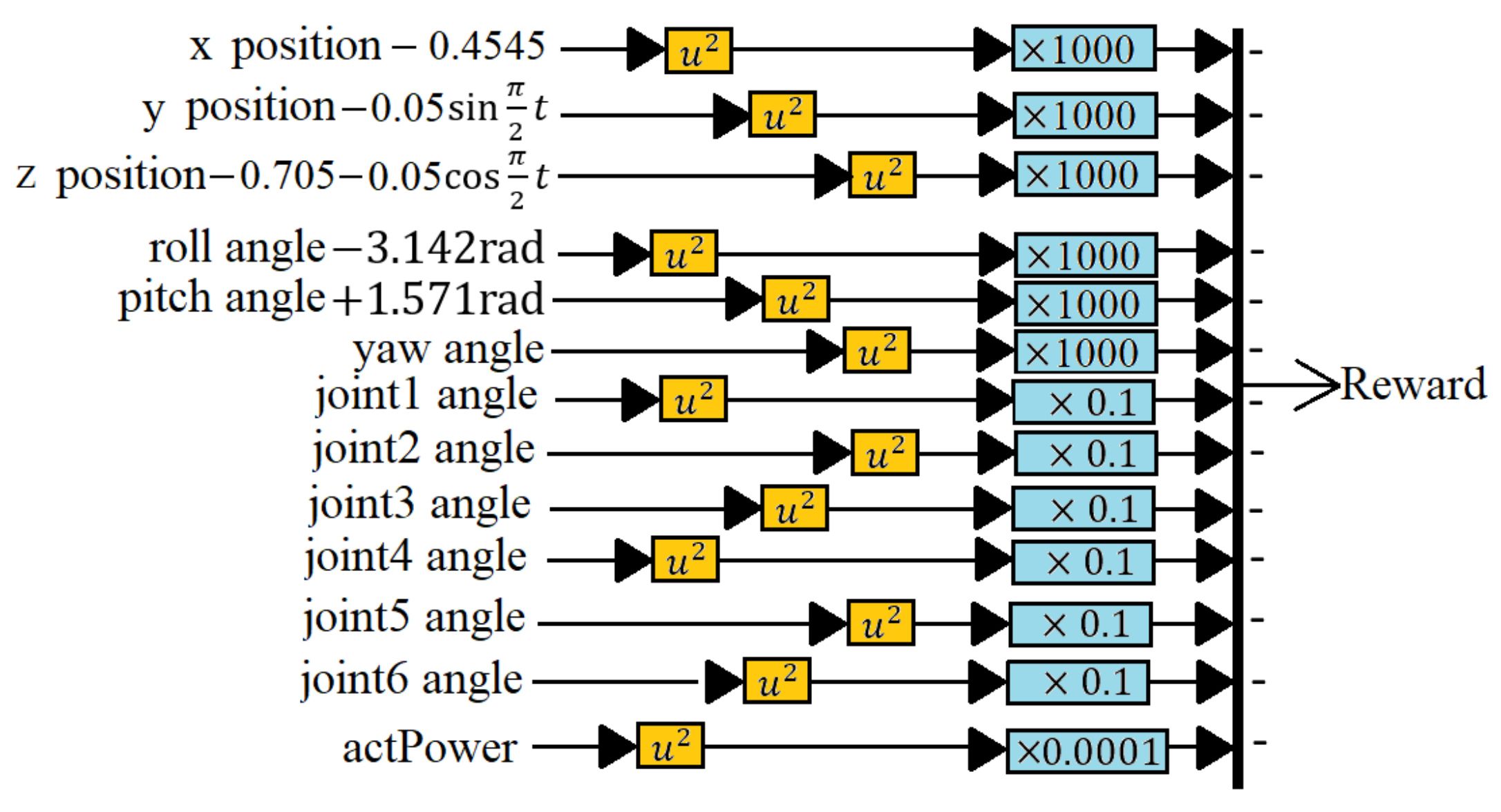
It is now easy to use the RL blocks for training, as shown in Figure 3, consisting of the Observation, Reward, Agent, Robot, and Sensor block. The Observation block receives the resultant states reflecting the attitude of the end effector with 43 inputs, as shown in Figure 4. The Reward block diagram receives the result states and calculates the reward, as shown in Figure 5. The Agent gets the output from the Observation, Reward, and Check-If-Done block, updates the Q function and the function, and outputs the reaction torques to the robot. The Sensor computes the forward kinematics as the resulting states and feeds it back to the three blocks.
4. Model Predictive Control [11,12]
As described before, MPC is based on the system dynamic model. The robot is described by Equation (9). Define the control law, Equation (10), to cancel the nonlinear effect:
The system reduces to a feedback-linearized system (11).
In the MPC, we apply a proportional-derivative (PD) controller given by Equation (12) to stabilize the robotic arm system:
where is the vector of joint variables to reflect the desired trajectory. Consider a time interval , where is the timeslot of the prediction. From Equation (10), we can develop the following two prediction models [12]:
If the target joint angle is , a simplified MPC design is to define a one-horizon time quadratic cost function to stabilize the system as:
where is the predicted angular position error, and is the predicted angular velocity error. In Equation (7), the timeslot and weight are positive real control parameters to be designed. To minimize , one introduces the prediction model Equation (13) into Equation (14) and lets the partial derivative equal 0. Considering that the robot slowly follows the trajectory, the resulting control becomes:
where and are:
By allowing the target joint angle to change over time, and from Equation (8), we obtain a more general control law:
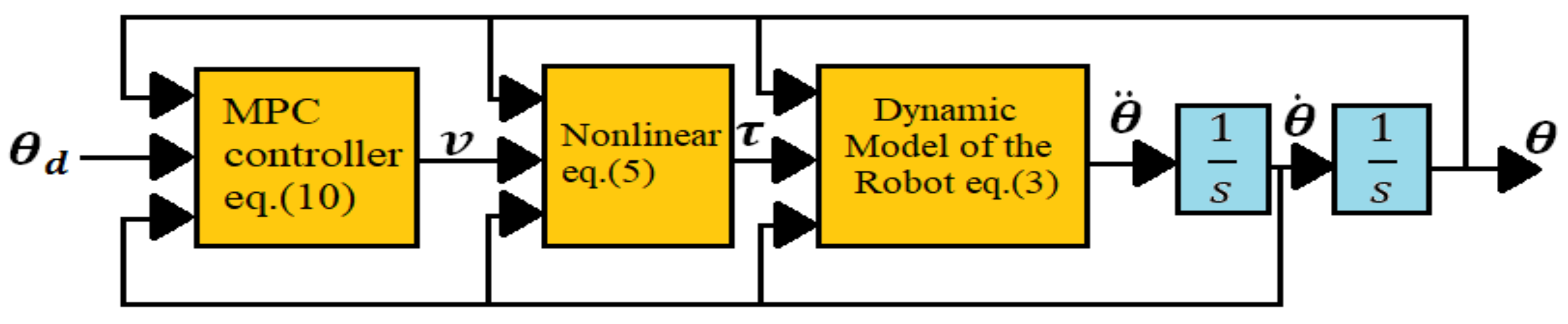
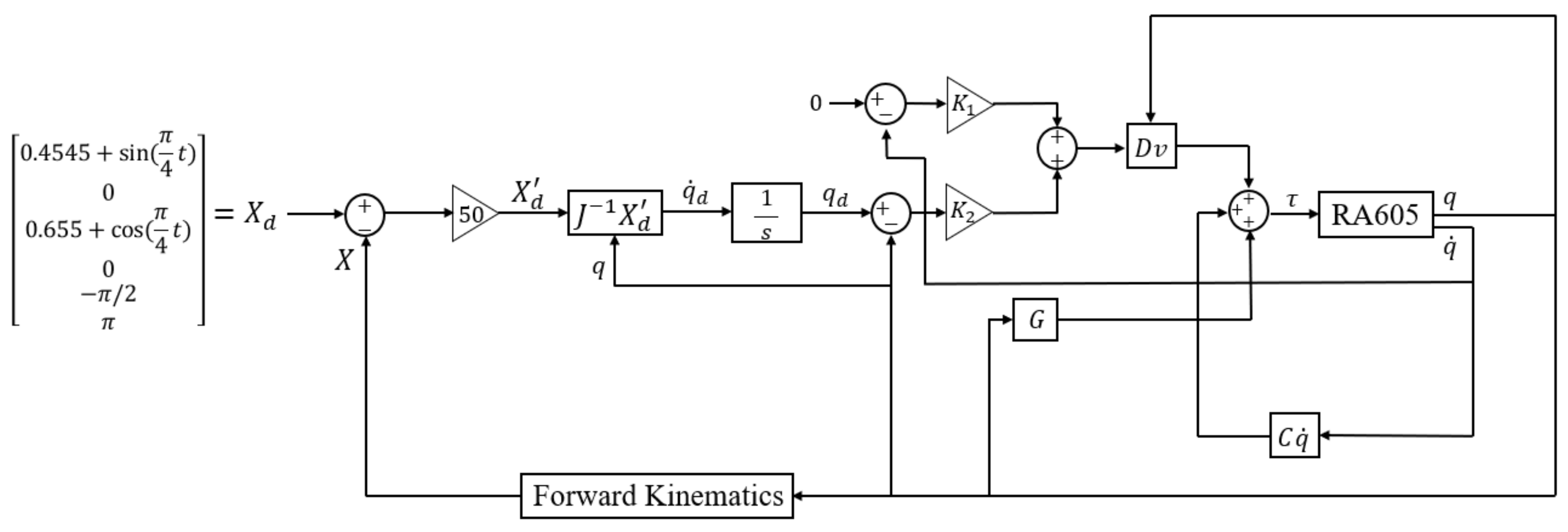
From Equations (9), (10), and (18), a block diagram of the MPC controller and the robotic arm system can be shown in Figure 6, where are the target joint angles in the joint-space.
The main goal of the control is for the joint angles to follow their targets according to the second-order dynamics specified by the transfer function , where is a damping factor and is a natural frequency by design.
Modeling of the Robotic Arm System
The HIWIN Technologies Corporation provided the RA605 robot arm for the D-H table, which can be readily incorporated into the “rvctools” Robotics toolbox in MATLAB for simulation purposes. It is also possible to obtain the system parameters for the dynamic model of the robot.
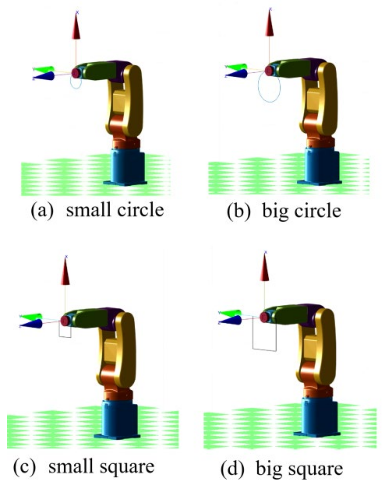
This research applied the DDPG to the RL training algorithm. We built an RA605 robotic arm model within the MATLAB simulation environment and, for generality purposes, four different target trajectories: a small circle trajectory (0.1 m diameter), a larger circle trajectory (0.2 m diameter), a small square trajectory (0.1 m side length) and a big square trajectory (0.2 m side length), Figure 7. To demonstrate the ability of six-axis trajectory control, we fixed the roll, pitch, and yaw angles of the end effector at , , and 0 rad, respectively.
5. The Control Results
This section compares the control performance of the RL and MPC trajectory controls.
5.1. The RL Training Results
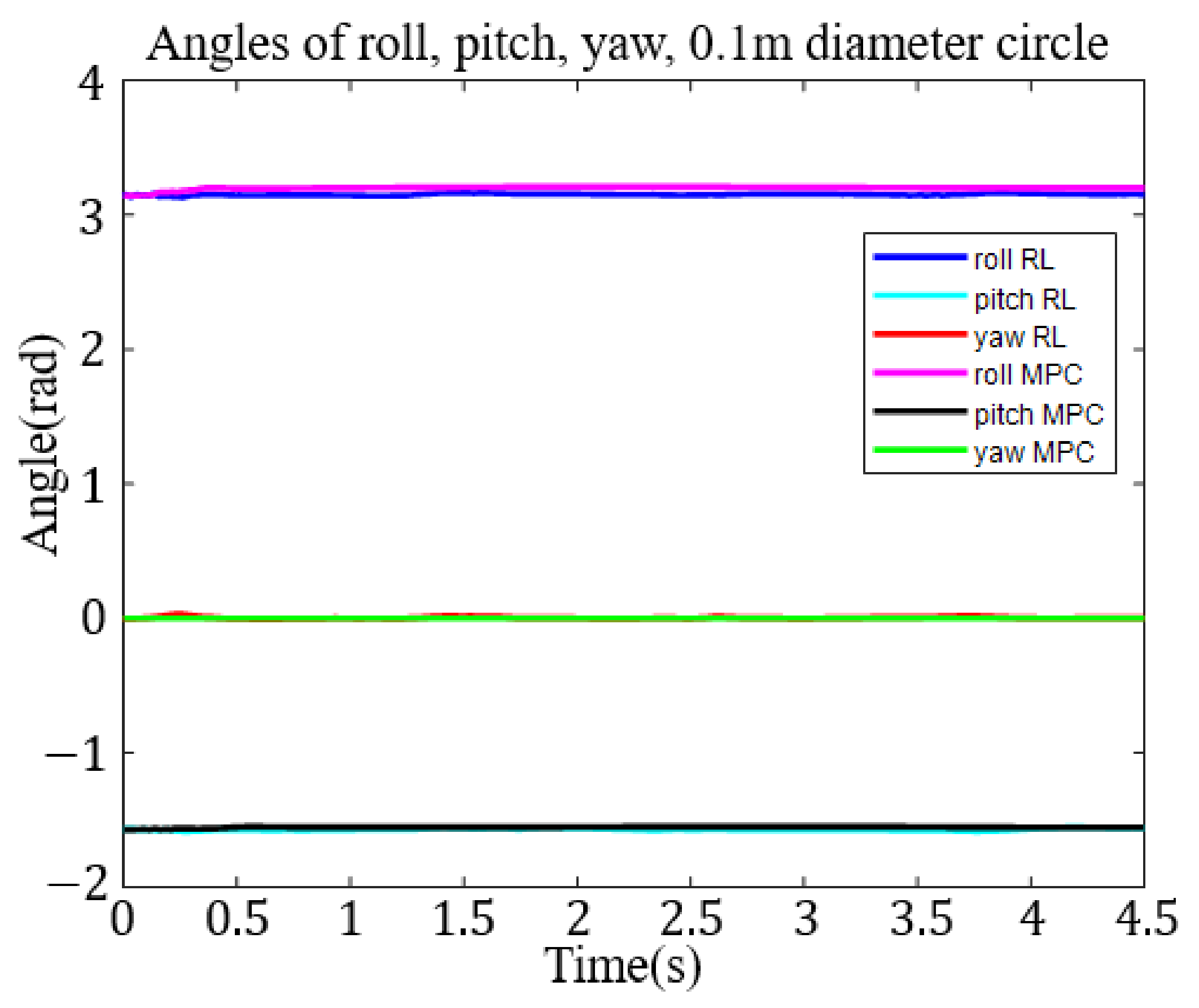
The 0.1 m diameter circle trajectory took about 343,070 s to train on an i7-computer running GPU and had 22,228 episodes. Figure 8 shows the roll, pitch, and yaw angle tracking results in the task space.
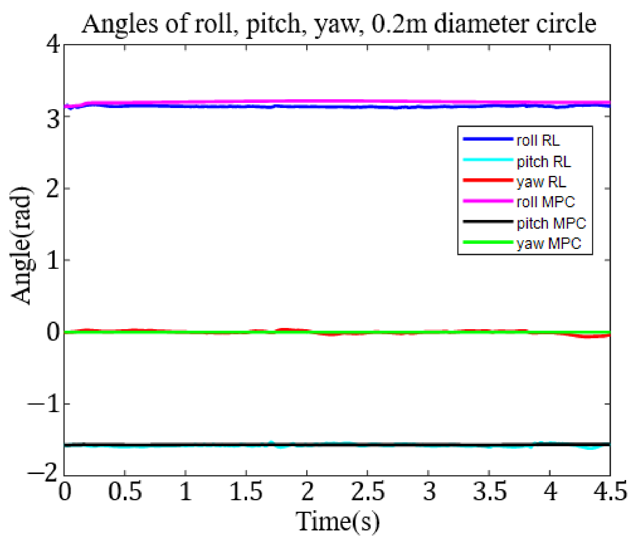
The 0.2 m diameter circle trajectory took a shorter 65,783 s and 4378 episodes to train. The roll, pitch, and yaw angle tracking results in the task space are shown in Figure 9.
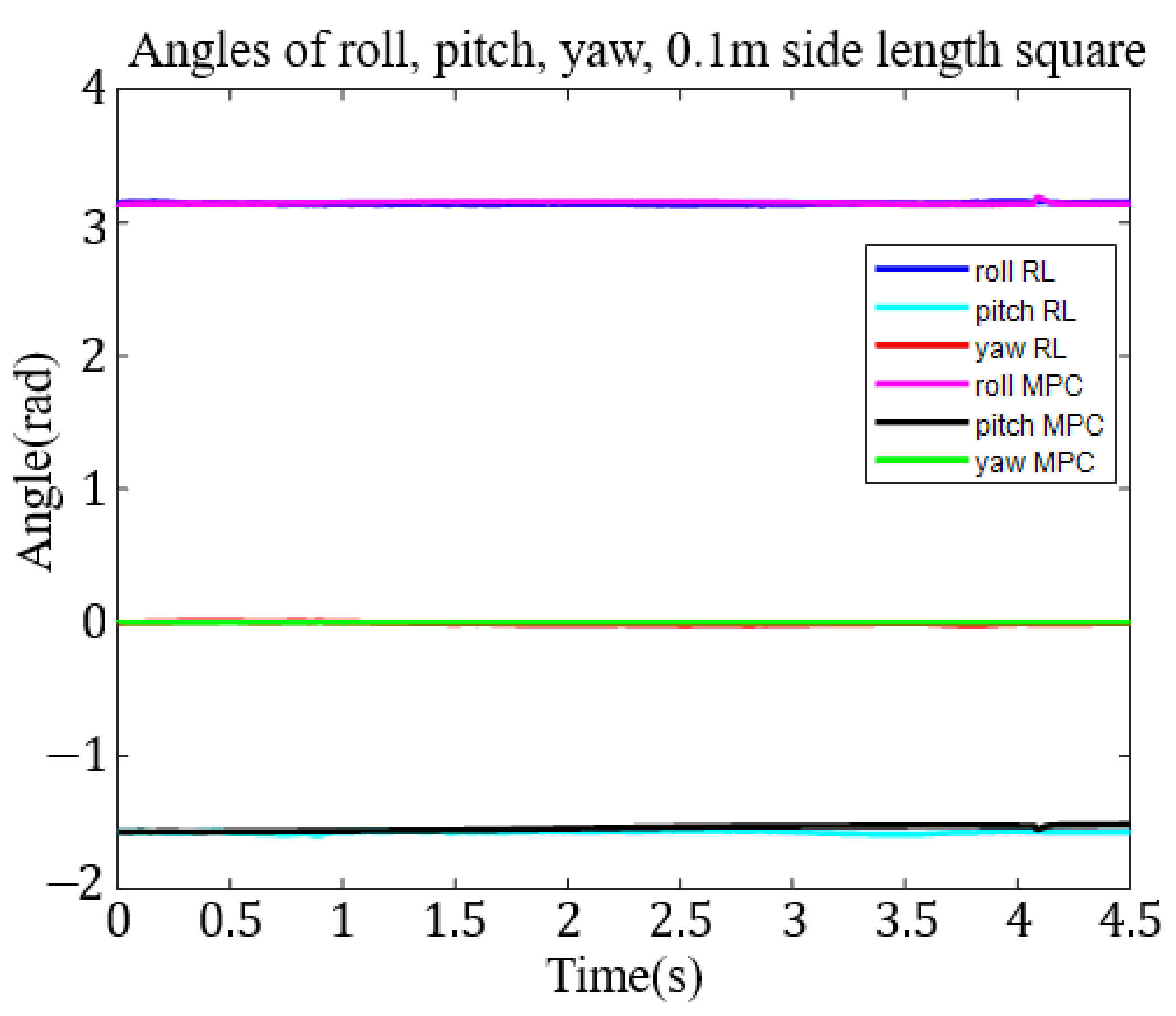
The 0.1 m square trajectory converged after training for about 186,100 s and 12,284 episodes. In Figure 10, we show the roll, pitch, and yaw angle tracking results in the task space.
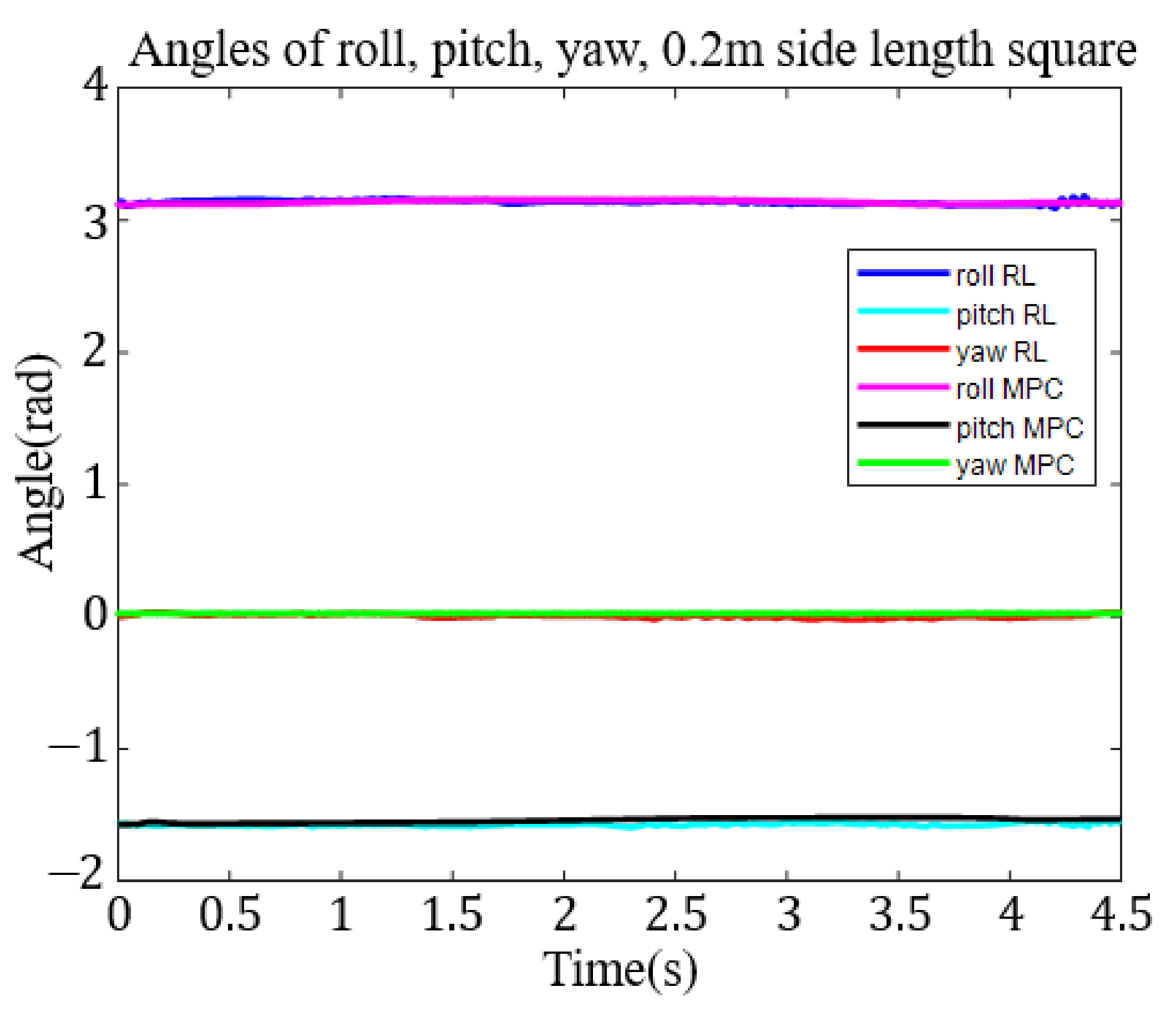
The 0.2 m square trajectory took about 129,040 s and 8338 episodes to train. In Figure 11, we show the roll, pitch, and yaw angle tracking results in the task space.
5.2. The Twin Delayed Deep Deterministic Policy Gradient Training
The authors also constructed a Twin Delayed Deep Deterministic Policy Gradient (TD3) network for comparison purposes. The network took 25,000 episodes to reach stable control. Figure 12 shows the resulting response. The robot arm’s trajectory follows a short 7.5 mm vertical line. As one observes from the result, Figure 12, the robot arm moved too fast and oscillated around a position with a 30 mm offset.
5.3. The MPC Results
For the MPC, we selected and to achieve a closed-loop bandwidth of and for no oscillation. From Equation (17), , .
The block diagram for the control system is shown in Figure 13. The MPC controller consists of the inverse dynamic calculation and uses the values of , , and for the input and the joint torques for the output. The parameter is the constant angular acceleration produced by the MPC controller. Four different target trajectories are shown in Figure 14.
For comparison, we ran the same trajectories as in the previous tests. The roll, pitch, and yaw angles in the task space are set at ,, and 0 rad, respectively. The motion is constrained to a slow speed.
To compare with the RL method easily, we put the result of MPC together with the RL method. For the 0.1 m diameter circle trajectory, we show the roll, pitch, and yaw angle tracking results in the task space in Figure 8. Figure 9 shows 0.2 m diameter circle roll, pitch, and yaw angle tracking results in the task space. The results for the 0.1 m square trajectory are shown in Figure 10. Again, Figure 10 shows the roll-pitch-yaw trajectories. Finally, the results for the 0.2 m square target trajectory are shown in Figure 11. The roll-pitch-yaw angle tracking results are shown in Figure 11.
5.4. The Comparison of RL and MPC
Table 1, Table 2 and Table 3 show the comparison for the roll-pitch-yaw angle tracking effect for the 0.1 m circular trajectory. Table 4, Table 5 and Table 6 show the comparison for the 0.2 m diameter circular trajectory roll-pitch-yaw errors. For the 0.1 m square target trajectory, Table 7, Table 8 and Table 9 show the comparison of the attitude errors. Likewise, Table 10, Table 11 and Table 12 compare the tracking results of the 0.2 m square trajectory.
From Table 1, Table 2, Table 3, Table 4, Table 5, Table 6, Table 7, Table 8 and Table 9, most (88%) of the absolute values of the roll-pitch-yaw angular errors resulting from the MPC are smaller than the corresponding errors resulting from the RL control. That means the MPC can track the designed trajectory better than the RL method. However, in Table 10, Table 11 and Table 12, most (83%) of the roll-pitch-yaw show larger errors by MPC, indicating that MPC is not as effective in controlling end effector attitude.
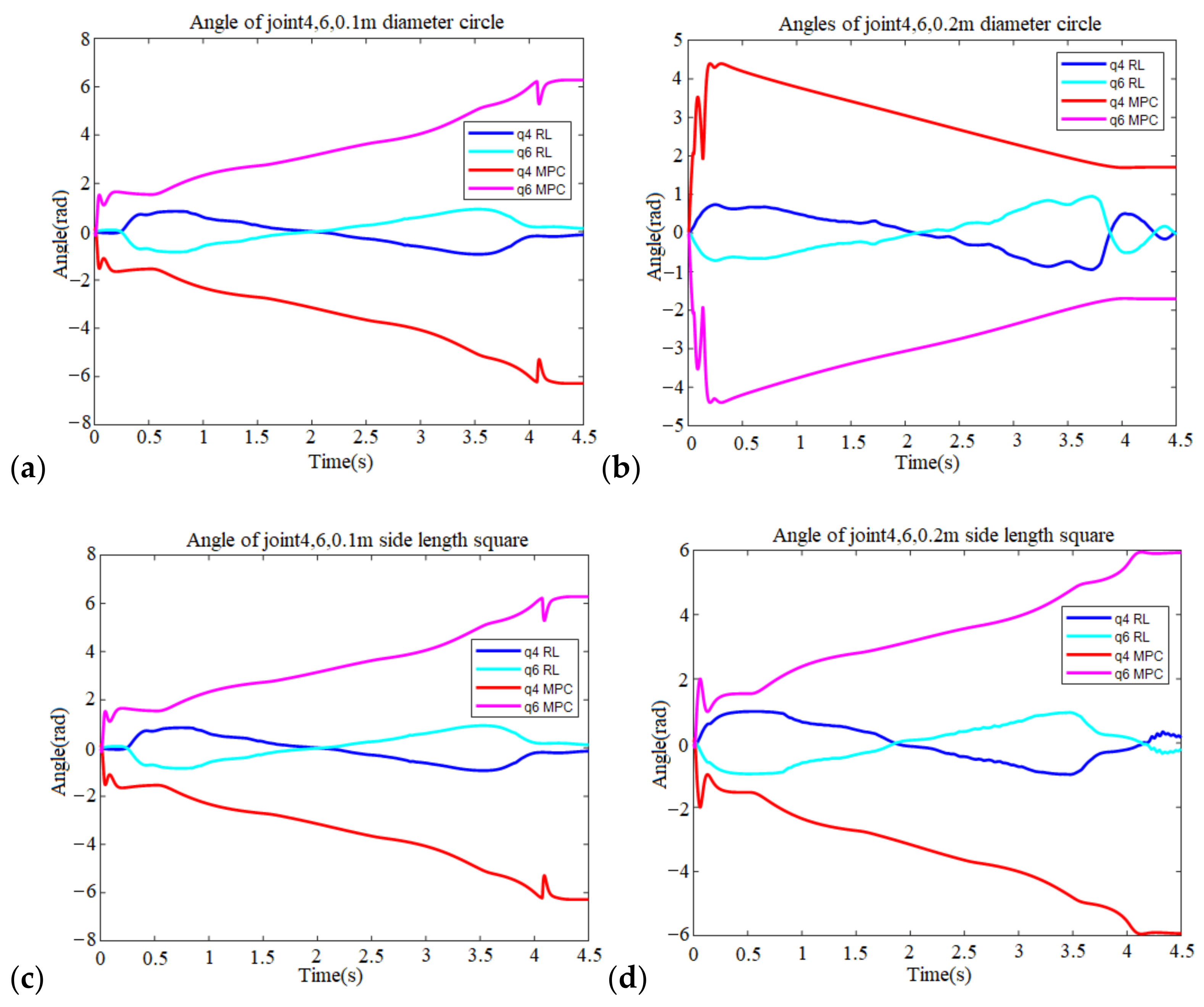
Furthermore, looking at this experimental result, one finds that the MPC drives joints 4 and 6 into very strenuous movements and does not restore to the original position, as shown in Figure 15. After examining the trajectory, one sees that the target trajectory passes through the vicinity of the singularity. The model-based control cannot avoid violent action without further treatment. The RL control, on the other hand, instinctively avoided these movements.
When the two methods are compared, it is clear that while the MPC is very effective in dealing with highly nonlinear system dynamics, it still necessitates the use of a model and additional treatment for singularities. On the other hand, the RL requires no prior knowledge of the underlying model and can drive the robotic arm through any trajectory. In addition, it is not affected by singularity. Furthermore, as the trajectory becomes larger and more complicated, the MPC no longer shows an advantage over the RL. This may be because the MPC cannot accurately calculate the attitude using the forward kinematics while the robotic six-joint angles become too large.
6. Conclusions
This paper proposes a split network structure for the direct application of RL to robotic trajectory following control. We first show that it is possible to train the RL network to directly mimic the inverse dynamic cancellation action without the help of a precise system model. The RL uses the modified DDPG algorithm as the underlying learning algorithm, and the tests follow four different target trajectories. The 0.1 m circle trajectory spent 343,070 s and 22,228 episodes training. It took 65,783 s and 4378 episodes to learn the 0.2 m circle trajectory. The 0.1 m square trajectory took 186,100 s to train, while the 0.2 m square trajectories took 129,040 s.
This study also compares RL performance to MPC performance. The RL control inherently avoids exercising violent movements while passing through the singularities and still succeeds in handling large and complicated trajectory situations. The MPC requires an accurate system model and is straightforward in implementation. However, it cannot avoid singularity without additional treatment and fails to control in large and complicated trajectory situations.
Comparing the two methods shows that RL successfully makes the robotic arm go through the target trajectory without excessive joint angle movements. MPC does not need time for training and achieves smoother control, but it requires an accurate system model. The authors will also try to implement the controller in an experiment for future verification.
Author Contributions
Conceptualization, C.-H.T. and J.-Y.Y.; methodology, C.-H.T. and J.-Y.Y.; software, C.-H.T., J.-J.L. and T.-F.H.; validation, C.-H.T., J.-J.L. and T.-F.H.; formal analysis, C.-H.T.; investigation, J.-J.L.; resources, J.-Y.Y.; data curation, C.-H.T.; writing—original draft preparation, C.-H.T.; writing—review and editing, J.-J.L. and J.-Y.Y.; visualization, J.-Y.Y.; supervision, J.-Y.Y.; project administration, J.-Y.Y.; funding acquisition, J.-Y.Y. All authors have read and agreed to the published version of the manuscript.
Funding
This research is supported by the National Science and Technology Council, Taiwan, under license no. MOST 108-2221-E-011 -166 -MY3.
Institutional Review Board Statement
Not applicable.
Informed Consent Statement
Not applicable.
Data Availability Statement
No new data were created or analyzed in this study. Data sharing is not applicable to this article.
Conflicts of Interest
The authors declare no conflict of interest.
References
- Luo, J.; Solowjow, E.; Wen, C.; Ojea, J.A.; Agogino, A.M. Deep Reinforcement Learning for Robotic Assembly of Mixed Deformable and Rigid Objects. In Proceedings of the 2018 IEEE/RSJ International Conference on Intelligent Robots and Systems (IROS), Madrid, Spain, 1–5 October 2018. [Google Scholar]
- Singh, A.; Nandi, G.C. Machine Learning based Joint Torque calculations of Industrial Robots. In Proceedings of the 2018 Conference on Information and Communication Technology (CICT), Jabalpur, India, 26–28 October 2018. [Google Scholar]
- Díaz-Tena, E.; Ugalde, U.; de Lacalle, L.N.L.; de la Iglesia, A.; Calleja, A.; Campa, F.J. Propagation of assembly errors in multitasking machines by the homogenous matrix method. Int. J. Adv. Manuf. Technol. 2013, 68, 149–164. [Google Scholar] [CrossRef]
- Nuttin, M.; Van Brussel, H. Learning the peg-into-hole assembly operation with a connectionist reinforcement technique. Comput. Ind. 1997, 33, 101–109. [Google Scholar] [CrossRef]
- Schaal, S. Learning from demonstration. In Advances in Neural Information Processing Systems; Morgan Kaufmann Publishers Inc.: San Francisco, CA, USA, 1997. [Google Scholar]
- Peters, J.; Schaal, S. Policy gradient methods for robotics. In Proceedings of the 2006 IEEE/RSJ International Conference on Intelligent Robots and Systems, Beijing, China, 9–15 October 2006. [Google Scholar]
- Peters, J.; Schaal, S. Reinforcement learning by reward-weighted regression for operational space control. In Proceedings of the 24th International Conference on Machine Learning, Corvalis, OR, USA, 20–24 June 2007. [Google Scholar]
- Kober, J.; Oztop, E.; Peters, J. Reinforcement learning to adjust robot movements to new situations. In Proceedings of the Twenty-Second International Joint Conference on Artificial Intelligence, Barcelona, Spain, 16–22 July 2011. [Google Scholar]
- Gu, S.; Holly, E.; Lillicrap, T.; Levine, S. Deep reinforcement learning for robotic manipulation with asynchronous off-policy updates. In Proceedings of the 2017 IEEE International Conference on Robotics and Automation (ICRA), Singapore, 29 May–3 June 2017. [Google Scholar]
- Liu, S.; Li, Y.-F.; Xing, D.-P.; Xu, D.; Su, H. An Efficient Insertion Control Method for Precision Assembly of Cylindrical Components. IEEE Trans. Ind. Electron. 2017, 64, 9355–9365. [Google Scholar] [CrossRef]
- Silver, D.; Lever, G.; Heess, N.; Degris, T.; Wierstra, D.; Riedmiller, M. Deterministic policy gradient algorithms. In Proceedings of the 31st International Conference on Machine Learning, Beijing, China, 21–26 June 2014. [Google Scholar]
- Kormushev, P.; Calinon, S.; Caldwell, D.G. Reinforcement Learning in Robotics: Applications and Real-World Challenges. Robotics 2013, 2, 122–148. [Google Scholar] [CrossRef] [Green Version]
- Wang, X.; Wang, S.; Liang, X.; Zhao, D.; Huang, J.; Xu, X.; Dai, B.; Miao, Q. Deep reinforcement learning: A survey. Front. Inf. Technol. Electron. Eng. 2020, 21, 1726–1744. [Google Scholar] [CrossRef]
- Lillicrap, T.P.; Hunt, J.J.; Pritzel, A.; Heess, N.; Erez, T.; Tassa, Y.; Silver, D.; Wierstra, D. Continuous control with deep reinforcement learning. In Proceedings of the 4th International Conference on Learning Representations, ICLR 2016—Conference Track Proceedings, San Juan, Puerto Rico, 2–4 May 2016. [Google Scholar]
- Van Hasselt, H.; Guez, A.; Silver, D. Deep reinforcement learning with double Q-Learning. In Proceedings of the 30th AAAI Conference on Artificial Intelligence (AAAI 2016), Phoenix, AZ, USA, 12–17 February 2016. [Google Scholar]
- Ansehel, O.; Baram, N.; Shimkin, N. Averaged-DQN: Variance reduction and stabilization for Deep Reinforcement Learning. In Proceedings of the 34th International Conference on Machine Learning, Sydney, Australia, 6–11 August 2017. [Google Scholar]
- Lee, D.; Defourny, B.; Powell, W.B. Bias-corrected Q-learning to control max-operator bias in Q-learning. In Proceedings of the 2013 IEEE Symposium on Adaptive Dynamic Programming and Reinforcement Learning (ADPRL), Singapore, 16–19 April 2013. [Google Scholar]
- He, F.S.; Liu, Y.; Schwing, A.G.; Peng, J. Learning to play in a day: Faster deep reinforcement learning by optimality tightening. In Proceedings of the 5th International Conference on Learning Representations, ICLR 2017—Conference Track Proceedings, Toulon, France, 24–26 April 2017. [Google Scholar]
- Nachum, O.; Norouzi, M.; Tucker, G.; Schuurmans, D. Smoothed action value functions for learning Gaussian policies. In Proceedings of the 35th International Conference on Machine Learning, Stockholm, Sweden, 10–15 July 2018. [Google Scholar]
- De Asis, K.; Hernandez-Garcia, J.; Holland, G.; Sutton, R. Multi-step reinforcement learning: A unifying algorithm. In Proceedings of the 32nd AAAI Conference on Artificial Intelligence (AAAI 2018), New Orleans, LA, USA, 2–7 February 2018. [Google Scholar]
- Al-Dabooni, S.; Wunsch, D.C. An Improved N-Step Value Gradient Learning Adaptive Dynamic Programming Algorithm for Online Learning. IEEE Trans. Neural Netw. Learn. Syst. 2020, 31, 1155–1169. [Google Scholar] [CrossRef] [PubMed]
- Wang, D.; Hu, M. Deep Deterministic Policy Gradient With Compatible Critic Network. IEEE Trans. Neural Netw. Learn. Syst. 2021, 1–13. [Google Scholar] [CrossRef] [PubMed]
- Ghavamzadeh, M.; Mahadevan, S. Continuous-Time Hierarchical Reinforcement Learning. In Proceedings of the Eighteenth International Conference on Machine Learning, Williamstown, MA, USA, 28 June–1 July 2001; pp. 186–193. [Google Scholar]
- Tiganj, Z.; Shankar, K.H.; Howard, M.W. Scale invariant value computation for reinforcement learning in continuous time. In Proceedings of the AAAI Spring Symposium, Palo Alto, CA, USA, 24–25 March 1997. [Google Scholar]
- Jiao, Z.; Oh, J. A Real-Time Actor-Critic Architecture for Continuous Control. In Trends in Artificial Intelligence Theory and Applications. Artificial Intelligence Practices; Springer International Publishing: Cham, Switzerland, 2020. [Google Scholar]
- Chen, S.; Wen, J. Industrial Robot Trajectory Tracking Control Using Multi-Layer Neural Networks Trained by Iterative Learning Control. Robotics 2021, 10, 50. [Google Scholar] [CrossRef]
- Kwon, W.H.; Bruckstein, A.M.; Kailath, T. Stabilizing state-feedback design via the moving horizon method. Int. J. Control 1983, 37, 631–643. [Google Scholar] [CrossRef]
- Nikdel, N.; Nikdel, P.; Badamchizadeh, M.A.; Hassanzadeh, I. Using Neural Network Model Predictive Control for Controlling Shape Memory Alloy-Based Manipulator. IEEE Trans. Ind. Electron. 2014, 61, 1394–1401. [Google Scholar] [CrossRef]
- García, C.E.; Prett, D.M.; Morari, M. Model predictive control: Theory and practice—A survey. Automatica 1989, 25, 335–348. [Google Scholar] [CrossRef]
- Ersdal, A.M.; Fabozzi, D.; Imsland, L.; Thornhill, N.F. Model Predictive Control for Power System Frequency Control Taking into Account Imbalance Uncertainty. IFAC Proc. Vol. 2014, 47, 981–986. [Google Scholar] [CrossRef] [Green Version]
- Chen, J.; Tang, C.; Xin, L.; Li, S.E.; Tomizuka, M. Continuous Decision Making for On-road Autonomous Driving under Uncertain and Interactive Environments. In Proceedings of the 2018 IEEE Intelligent Vehicles Symposium (IV), Changshu, China, 26–30 June 2018. [Google Scholar]
- Tang, Q.; Chu, Z.; Qiang, Y.; Wu, S.; Zhou, Z. Trajectory Tracking of Robotic Manipulators with Constraints Based on Model Predictive Control. In Proceedings of the 2020 17th International Conference on Ubiquitous Robots (UR), Kyoto, Japan, 22–26 June 2020. [Google Scholar]
- Lu, C.; Wang, K.; Xu, H. Trajectory Tracking of Manipulators Based on Improved Robust Nonlinear Predictive Control. In Proceedings of the 2020 1st International Conference on Control, Robotics and Intelligent System, Xiamen, China, 27–29 October 2020. [Google Scholar]
- Abbas, H.S.; Cisneros, P.S.G.; Mannel, G.; Rostalski, P.; Werner, H. Practical Model Predictive Control for a Class of Nonlinear Systems Using Linear Parameter-Varying Representations. IEEE Access 2021, 9, 62380–62393. [Google Scholar] [CrossRef]
- Best, C.M.; Gillespie, M.T.; Hyatt, P.; Rupert, L.; Sherrod, V.; Killpack, M.D. A New Soft Robot Control Method: Using Model Predictive Control for a Pneumatically Actuated Humanoid. IEEE Robot. Autom. Mag. 2016, 23, 75–84. [Google Scholar] [CrossRef]
- Lunni, D.; Santamaria-Navarro, A.; Rossi, R.; Rocco, P.; Bascetta, L.; Andrade-Cetto, J. Nonlinear model predictive control for aerial manipulation. In Proceedings of the 2017 International Conference on Unmanned Aircraft Systems (ICUAS), Miami, FL, USA, 13–16 June 2017. [Google Scholar]
- Guechi, E.-H.; Bouzoualegh, S.; Zennir, Y.; Blažič, S. MPC Control and LQ Optimal Control of A Two-Link Robot Arm: A Comparative Study. Machines 2018, 6, 37. [Google Scholar] [CrossRef]
- Guechi, E.H.; Bouzoualegh, S.; Messikh, L.; Blažic, S. Model predictive control of a two-link robot arm. In Proceedings of the 2018 International Conference on Advanced Systems and Electric Technologies (IC_ASET), Hammamet, Tunisia, 22–25 March 2018. [Google Scholar]
- Car, M.; Ivanovic, A.; Orsag, M.; Bogdan, S. Impedance Based Force Control for Aerial Robot Peg-in-Hole Insertion Tasks. In Proceedings of the 2018 IEEE/RSJ International Conference on Intelligent Robots and Systems (IROS), Madrid, Spain, 1–5 October 2018. [Google Scholar]
Figure 1.
The neural network system of the agent.

Figure 2.
The neural network system of the critic.

Figure 3.
The training block diagram.

Figure 4.
The Observation block.

Figure 5.
The Reward block.

Figure 6.
The MPC controller and the robot arm system.

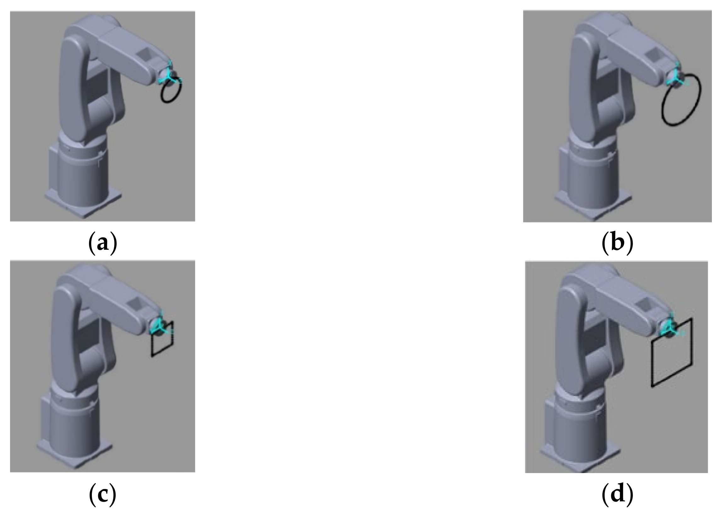
Figure 7.
(a) small circle trajectory (b) big circle trajectory (c) small square trajectory (d) big square trajectory.
Figure 7.
(a) small circle trajectory (b) big circle trajectory (c) small square trajectory (d) big square trajectory.

Figure 8.
The angles of roll, pitch, and yaw of the end of the robotic arm (RL and MPC, 0.1 m diameter circle).
Figure 8.
The angles of roll, pitch, and yaw of the end of the robotic arm (RL and MPC, 0.1 m diameter circle).

Figure 9.
The angles of roll, pitch, and yaw of the end of the robotic arm (RL and MPC, 0.2 m diameter circle).
Figure 9.
The angles of roll, pitch, and yaw of the end of the robotic arm (RL and MPC, 0.2 m diameter circle).

Figure 10.
The angles of roll, pitch, and yaw of the end of robotic arm (RL and MPC, 0.1 m side length square).
Figure 10.
The angles of roll, pitch, and yaw of the end of robotic arm (RL and MPC, 0.1 m side length square).

Figure 11.
The angles of roll, pitch, and yaw of the end of the robotic arm (RL and MPC, 0.2 m side length square).
Figure 11.
The angles of roll, pitch, and yaw of the end of the robotic arm (RL and MPC, 0.2 m side length square).

Figure 12.
Trajectory following results for a Twin Delayed Deep Deterministic Policy Gradient network. (to follow a vertical line of 7.5 mm).
Figure 12.
Trajectory following results for a Twin Delayed Deep Deterministic Policy Gradient network. (to follow a vertical line of 7.5 mm).

Figure 13.
The block diagram of the MPC controller of the RA605 robotic arm.

Figure 14.
(a) small circle trajectory (b) big circle trajectory (c) small square trajectory (d) big square trajectory.
Figure 14.
(a) small circle trajectory (b) big circle trajectory (c) small square trajectory (d) big square trajectory.

Figure 15.
(a) The joint angles of four and six of the robotic arm (MPC vs. RL, 0.1 m diameter circle); (b) The joint angles of four and six of the robotic arm (MPC vs. RL, 0.2 m diameter circle); (c) The joint angles of four and six of the robotic arm (MPC vs. RL, 0.1 m side length square); and (d) The joint angles of four and six of the robotic arm (MPC vs. RL, 0.2 m side length square).


Table 1.
The roll angle of the end of the robotic arm (0.1 m circle).
| Time (s) | Roll_MPC (Rad) | Roll_RL (Rad) | Roll_Demand (Rad) | Error_MPC (Rad) | Error_RL (Rad) |
|---|---|---|---|---|---|
| 0 | 3.14 | 3.14 | 3.14 | 4.07 × 10⁻⁴ | 1.43 × 10⁻⁴ |
| 0.5 | 3.14 | 3.14 | 3.14 | 3.87 × 10⁻⁴ | −8.90 × 10⁻⁴ |
| 1 | 3.14 | 3.14 | 3.14 | 4.33 × 10⁻⁴ | −4.98 × 10⁻³ |
| 1.5 | 3.14 | 3.13 | 3.14 | 3.96 × 10⁻⁴ | −8.74 × 10⁻³ |
| 2 | 3.14 | 3.14 | 3.14 | 3.61 × 10⁻⁴ | −5.75 × 10⁻³ |
| 2.5 | 3.14 | 3.15 | 3.14 | 4.83 × 10⁻⁴ | 4.35 × 10⁻³ |
| 3 | 3.14 | 3.14 | 3.14 | 4.21 × 10⁻⁴ | 6.84 × 10⁻⁴ |
| 3.5 | 3.14 | 3.14 | 3.14 | 3.29 × 10⁻⁴ | −1.58 × 10⁻⁴ |
| 4 | 3.14 | 3.14 | 3.14 | 4.37 × 10⁻⁴ | −4.29 × 10⁻⁴ |
| 4.5 | 3.14 | 3.14 | 3.14 | 4.88 × 10⁻⁴ | 1.37 × 10⁻³ |
Table 2.
The pitch angle of the end of the robotic arm (0.1 m circle).
| Time (s) | Pitch_MPC (Rad) | Pitch_RL (Rad) | Pitch_Demand (Rad) | Error_MPC (Rad) | Error_RL (Rad) |
|---|---|---|---|---|---|
| 0 | −1.57 | −1.57 | −1.57 | 6.66 × 10⁻¹⁵ | −4.07 × 10⁻⁴ |
| 0.5 | −1.57 | −1.57 | −1.57 | 7.67 × 10⁻⁴ | −7.58 × 10⁻⁴ |
| 1 | −1.57 | −1.57 | −1.57 | 7.87 × 10⁻⁴ | −2.18 × 10⁻³ |
| 1.5 | −1.57 | −1.57 | −1.57 | 8.05 × 10⁻⁴ | −1.74 × 10⁻³ |
| 2 | −1.57 | −1.57 | −1.57 | 8.11 × 10⁻⁴ | −3.28 × 10⁻³ |
| 2.5 | −1.57 | −1.57 | −1.57 | 8.05 × 10⁻⁴ | 1.45 × 10⁻³ |
| 3 | −1.57 | −1.57 | −1.57 | 7.89 × 10⁻⁴ | −1.96 × 10⁻⁴ |
| 3.5 | −1.57 | −1.58 | −1.57 | 7.69 × 10⁻⁴ | −4.39 × 10⁻³ |
| 4 | −1.57 | −1.56 | −1.57 | 7.23 × 10⁻⁴ | 7.04 × 10⁻³ |
| 4.5 | −1.57 | −1.57 | −1.57 | 7.96 × 10⁻⁴ | 6.37 × 10⁻⁴ |
Table 3.
The yaw angle of the end of the robotic arm (0.1 m circle).
| Time (s) | Yaw_MPC (Rad) | Yaw_RL (Rad) | Yaw_Demand (Rad) | Error_MPC (Rad) | Error_RL (Rad) |
|---|---|---|---|---|---|
| 0 | 7.36 × 10⁻¹⁵ | −2.05 × 10⁻⁴ | 0 | 7.36 × 10⁻¹⁵ | −2.05 × 10⁻⁴ |
| 0.5 | −9.65 × 10⁻⁵ | 8.12 × 10⁻³ | 0 | −9.65 × 10⁻⁵ | 8.12 × 10⁻³ |
| 1 | 9.61 × 10⁻⁵ | 2.68 × 10⁻³ | 0 | 9.61 × 10⁻⁵ | 2.68 × 10⁻³ |
| 1.5 | −3.96 × 10⁻⁵ | 9.70 × 10⁻⁴ | 0 | −3.96 × 10⁻⁵ | 9.70 × 10⁻⁴ |
| 2 | −5.90 × 10⁻⁵ | 3.90 × 10⁻³ | 0 | −5.90 × 10⁻⁵ | 3.90 × 10⁻³ |
| 2.5 | 2.90 × 10⁻⁵ | 7.66 × 10⁻⁴ | 0 | 2.90 × 10⁻⁵ | 7.66 × 10⁻⁴ |
| 3 | 3.38 × 10⁻⁵ | −8.37 × 10⁻³ | 0 | 3.38 × 10⁻⁵ | −8.37 × 10⁻³ |
| 3.5 | −8.86 × 10⁻⁵ | −7.24 × 10⁻³ | 0 | −8.8 × 10⁻⁵ | −7.24 × 10⁻³ |
| 4 | 9.58 × 10⁻⁵ | 4.31 × 10⁻³ | 0 | 9.58 × 10⁻⁵ | 4.31 × 10⁻³ |
| 4.5 | 5.85 × 10⁻⁵ | −3.24 × 10⁻⁵ | 0 | 5.85 × 10⁻⁵ | −3.24 × 10⁻⁵ |
Table 4.
The roll angle of the end of the robotic arm (0.2 m circle).
| Time (s) | Roll_MPC (Rad) | Roll_RL (Rad) | Roll_Demand (Rad) | Error_MPC (Rad) | Error_RL (Rad) |
|---|---|---|---|---|---|
| 0 | 3.14 | 3.14 | 3.14 | 4.07 × 10⁻⁴ | 1.43 × 10⁻⁴ |
| 0.5 | 3.14 | 3.15 | 3.14 | 4.72 × 10⁻⁴ | 5.14 × 10⁻³ |
| 1 | 3.14 | 3.14 | 3.14 | 4.40 × 10⁻⁴ | −1.71 × 10⁻³ |
| 1.5 | 3.14 | 3.14 | 3.14 | 3.40 × 10⁻⁴ | −3.64 × 10⁻³ |
| 2 | 3.14 | 3.14 | 3.14 | 4.28 × 10⁻⁴ | −3.75 × 10⁻³ |
| 2.5 | 3.14 | 3.14 | 3.14 | 3.46 × 10⁻⁴ | −5.92 × 10⁻³ |
| 3 | 3.14 | 3.13 | 3.14 | 4.54 × 10⁻⁴ | −1.10 × 10⁻² |
| 3.5 | 3.14 | 3.15 | 3.14 | 3.25 × 10⁻⁴ | 8.85 × 10⁻³ |
| 4 | 3.14 | 3.14 | 3.14 | 4.59 × 10⁻⁴ | −6.69 × 10⁻⁴ |
| 4.5 | 3.14 | 3.15 | 3.14 | 4.75 × 10⁻⁴ | 6.82 × 10⁻³ |
Table 5.
The pitch angle of the end of the robotic arm (0.2 m circle).
| Time (s) | Pitch_MPC (Rad) | Pitch_RL (Rad) | Pitch_Demand (Rad) | Error_MPC (Rad) | Error_RL (Rad) |
|---|---|---|---|---|---|
| 0 | −1.57 | −1.57 | −1.57 | 6.66 × 10⁻¹⁵ | −4.07 × 10⁻⁴ |
| 0.5 | −1.57 | −1.60 | −1.57 | 6.66 × 10⁻⁴ | −2.44 × 10⁻² |
| 1 | −1.57 | −1.58 | −1.57 | 6.86 × 10⁻⁴ | −8.60 × 10⁻³ |
| 1.5 | −1.57 | −1.57 | −1.57 | 8.67 × 10⁻⁴ | −2.43 × 10⁻³ |
| 2 | −1.57 | −1.57 | −1.57 | 9.46 × 10⁻⁴ | −1.66 × 10⁻³ |
| 2.5 | −1.57 | −1.57 | −1.57 | 8.12 × 10⁻⁴ | −1.51 × 10⁻³ |
| 3 | −1.57 | −1.58 | −1.57 | 7.75 × 10⁻⁴ | −1.00 × 10⁻² |
| 3.5 | −1.57 | −1.60 | −1.57 | 6.23 × 10⁻⁴ | −2.93 × 10⁻² |
| 4 | −1.57 | −1.55 | −1.57 | 6.47 × 10⁻⁴ | 2.46 × 10⁻² |
| 4.5 | −1.57 | −1.57 | −1.57 | 7.96 × 10⁻⁴ | −1.13 × 10⁻³ |
Table 6.
The yaw angle of the end of the robotic arm (0.2 m circle).
| Time (s) | Yaw_MPC (Rad) | Yaw_RL (Rad) | Yaw_Demand (Rad) | Error_MPC (Rad) | Error_RL (Rad) |
|---|---|---|---|---|---|
| 0 | −3.64 × 10⁻¹⁴ | −2.05 × 10⁻⁴ | 0 | −3.64 × 10⁻¹⁴ | −2.05 × 10⁻⁴ |
| 0.5 | 6.45 × 10⁻⁵ | 1.66 × 10⁻² | 0 | 6.45 × 10⁻⁵ | 1.66 × 10⁻² |
| 1 | 3.30 × 10⁻⁵ | 1.90 × 10⁻³ | 0 | 3.30 × 10⁻⁵ | 1.90 × 10⁻³ |
| 1.5 | −6.78 × 10⁻⁵−5 | −5.11 × 10⁻³ | 0 | −6.78 × 10⁻⁵ | −5.11 × 10⁻³ |
| 2 | 2.04 × 10⁻⁵ | 1.51 × 10⁻² | 0 | 2.04 × 10⁻⁵ | 1.51 × 10⁻² |
| 2.5 | −6.10 × 10⁻⁵ | −7.64 × 10⁻³ | 0 | −6.10 × 10⁻⁵ | −7.64 × 10⁻³ |
| 3 | 4.69 × 10⁻⁵ | 1.97 × 10⁻³ | 0 | 4.69 × 10⁻⁵ | 1.97 × 10⁻³ |
| 3.5 | −8.21 × 10⁻⁵ | 1.38 × 10⁻² | 0 | −8.21 × 10⁻⁵ | 1.38 × 10⁻² |
| 4 | 5.19 × 10⁻⁵ | −6.25 × 10⁻³ | 0 | 5.19 × 10⁻⁵ | −6.25 × 10⁻³ |
| 4.5 | 6.77 × 10⁻⁵ | −3.48 × 10⁻² | 0 | 6.77 × 10⁻⁵ | −3.48 × 10⁻² |
Table 7.
The roll angle of the end of the robotic arm (0.1 m side length square).
| Time (s) | Roll_MPC (Rad) | Roll_RL (Rad) | Roll_Demand (Rad) | Error_MPC (Rad) | Error_RL (Rad) |
|---|---|---|---|---|---|
| 0 | 3.14 | 3.14 | 3.14 | 4.07 × 10⁻⁴ | 1.43 × 10⁻⁴ |
| 0.5 | 3.14 | 3.14 | 3.14 | 1.35 × 10⁻³ | 3.06 × 10⁻³ |
| 1 | 3.14 | 3.14 | 3.14 | 1.22 × 10⁻⁴ | 6.64 × 10⁻⁴ |
| 1.5 | 3.14 | 3.14 | 3.14 | 1.05 × 10⁻³ | 1.46 × 10⁻³ |
| 2 | 3.14 | 3.14 | 3.14 | −4.21 × 10⁻⁴ | 1.61 × 10⁻³ |
| 2.5 | 3.14 | 3.13 | 3.14 | 1.14 × 10⁻³ | −8.94 × 10⁻³ |
| 3 | 3.14 | 3.14 | 3.14 | 9.41 × 10⁻⁴ | −4.83 × 10⁻³ |
| 3.5 | 3.14 | 3.14 | 3.14 | 3.87 × 10⁻⁴ | 1.86 × 10⁻³ |
| 4 | 3.14 | 3.16 | 3.14 | 3.71 × 10⁻⁴ | 1.89 × 10⁻² |
| 4.5 | 3.14 | 3.15 | 3.14 | 6.34 × 10⁻⁴ | 1.13 × 10⁻² |
Table 8.
The pitch angle of the end of the robotic arm (0.1 m side length square).
| Time (s) | Pitch_MPC (Rad) | Pitch_RL (Rad) | Pitch_Demand (Rad) | Error_MPC (Rad) | Error_RL (Rad) |
|---|---|---|---|---|---|
| 0 | −1.57 | −1.57 | −1.57 | 6.66 × 10⁻¹⁵ | −4.07 × 10⁻⁴ |
| 0.5 | −1.57 | −1.58 | −1.57 | 7.73 × 10⁻⁴ | −6.96 × 10⁻³ |
| 1 | −1.57 | −1.57 | −1.57 | 6.29 × 10⁻⁴ | 1.10 × 10⁻⁵ |
| 1.5 | −1.57 | −1.57 | −1.57 | 7.50 × 10⁻⁴ | −3.08 × 10⁻³ |
| 2 | −1.57 | −1.57 | −1.57 | 1.00 × 10⁻³ | 5.17 × 10⁻³ |
| 2.5 | −1.57 | −1.56 | −1.57 | 1.02 × 10⁻³ | 1.08 × 10⁻² |
| 3 | −1.57 | −1.57 | −1.57 | 7.11 × 10⁻⁴ | 1.21 × 10⁻³ |
| 3.5 | −1.57 | −1.59 | −1.57 | 6.24 × 10⁻⁴ | −1.67 × 10⁻² |
| 4 | −1.57 | −1.57 | −1.57 | 7.10 × 10⁻⁴ | 5.29 × 10⁻³ |
| 4.5 | −1.57 | −1.57 | −1.57 | 7.82 × 10⁻⁴ | 3.52 × 10⁻⁴ |
Table 9.
The yaw angle of the end of the robotic arm (0.1 m side length square).
| Time (s) | Yaw_MPC (Rad) | Yaw_RL (Rad) | Yaw_Demand (Rad) | Error_MPC (Rad) | Error_RL (Rad) |
|---|---|---|---|---|---|
| 0 | 2.59 × 10⁻¹⁵ | −2.05 × 10⁻⁴ | 0 | 2.59 × 10⁻¹⁵ | −2.05 × 10⁻⁴ |
| 0.5 | 9.02 × 10⁻⁴ | 9.79 × 10⁻³ | 0 | 9.02 × 10⁻⁴ | 9.79 × 10⁻³ |
| 1 | −7.33 × 10⁻⁴ | 2.65 × 10⁻³ | 0 | −7.33 × 10⁻⁴ | 2.65 × 10⁻³ |
| 1.5 | 7.69 × 10⁻⁴ | −1.11 × 10⁻² | 0 | 7.69 × 10⁻⁴ | −1.11 × 10⁻² |
| 2 | −5.98 × 10⁻⁴ | −1.50 × 10⁻² | 0 | −5.98 × 10⁻⁴ | −1.50 × 10⁻² |
| 2.5 | 5.06 × 10⁻⁴ | −1.83 × 10⁻² | 0 | 5.06 × 10⁻⁴ | −1.83 × 10⁻² |
| 3 | 6.57 × 10⁻⁴ | −1.55 × 10⁻² | 0 | 6.57 × 10⁻⁴ | −1.55 × 10⁻² |
| 3.5 | −1.76 × 10⁻⁴ | −7.55 × 10⁻³ | 0 | −1.76 × 10⁻⁴ | −7.55 × 10⁻³ |
| 4 | −5.32 × 10⁻⁴ | −8.68 × 10⁻³ | 0 | −5.32 × 10⁻⁴ | −8.68 × 10⁻³ |
| 4.5 | 5.47 × 10⁻⁴ | −5.36 × 10⁻³ | 0 | 5.47 × 10⁻⁴ | −5.36 × 10⁻³ |
Table 10.
The roll angle of the end of the robotic arm (0.2 m side length square).
| Time (s) | Roll_MPC (Rad) | Roll_RL (Rad) | Roll_Demand (Rad) | Error_MPC (Rad) | Error_RL (Rad) |
|---|---|---|---|---|---|
| 0 | 3.14 | 3.14 | 3.14 | −2.49 × 10⁻¹⁴ | 1.43 × 10⁻⁴ |
| 0.5 | 3.12 | 3.15 | 3.14 | −2.21 × 10⁻² | 4.45 × 10⁻³ |
| 1 | 3.14 | 3.14 | 3.14 | 4.42 × 10⁻⁴ | −6.59 × 10⁻⁴ |
| 1.5 | 3.16 | 3.14 | 3.14 | 1.47 × 10⁻² | 1.31 × 10⁻³ |
| 2 | 3.15 | 3.15 | 3.14 | 1.08 × 10⁻² | 5.18 × 10⁻³ |
| 2.5 | 3.16 | 3.14 | 3.14 | 1.62 × 10⁻² | 1.17 × 10⁻³ |
| 3 | 3.14 | 3.15 | 3.14 | −2.24 × 10⁻³ | 9.98 × 10⁻³ |
| 3.5 | 3.12 | 3.16 | 3.14 | −1.67 × 10⁻² | 1.78 × 10⁻² |
| 4 | 3.12 | 3.16 | 3.14 | −1.88 × 10⁻² | 1.35 × 10⁻² |
| 4.5 | 3.13 | 3.16 | 3.14 | −8.64 × 10⁻³ | 1.46 × 10⁻² |
Table 11.
The pitch angle of the end of the robotic arm (0.2 m side length square).
| Time (s) | Pitch_MPC (Rad) | Pitch_RL (Rad) | Pitch_Demand (Rad) | Error_MPC (Rad) | Error_RL (Rad) |
|---|---|---|---|---|---|
| 0 | −1.57 | −1.57 | −1.57 | −3.55 × 10⁻¹⁵ | −4.07 × 10⁻⁴ |
| 0.5 | −1.56 | −1.58 | −1.57 | 6.06 × 10⁻³ | −1.12 × 10⁻² |
| 1 | −1.56 | −1.57 | −1.57 | 1.05 × 10⁻² | −2.60 × 10⁻³ |
| 1.5 | −1.55 | −1.55 | −1.57 | 1.63 × 10⁻² | 2.25 × 10⁻² |
| 2 | −1.54 | −1.55 | −1.57 | 2.91 × 10⁻² | 1.81 × 10⁻² |
| 2.5 | −1.53 | −1.57 | −1.57 | 4.42 × 10⁻² | 5.35 × 10⁻³ |
| 3 | −1.52 | −1.58 | −1.57 | 5.00 × 10⁻² | −5.54 × 10⁻³ |
| 3.5 | −1.52 | −1.58 | −1.57 | 5.12 × 10⁻² | −1.39 × 10⁻² |
| 4 | −1.53 | −1.57 | −1.57 | 4.13 × 10⁻² | −1.34 × 10⁻³ |
| 4.5 | −1.53 | −1.57 | −1.57 | 4.00 × 10⁻² | −1.21 × 10⁻³ |
Table 12.
The yaw angle of the end of the robotic arm (0.2 m side length square).
| Time (s) | Yaw_MPC (Rad) | Yaw_RL (Rad) | Yaw_Demand (Rad) | Error_MPC (Rad) | Error_RL (Rad) |
|---|---|---|---|---|---|
| 0 | 2.98 × 10⁻¹⁴ | −2.05 × 10⁻⁴ | 0 | 2.98 × 10⁻¹⁴ | −2.05 × 10⁻⁴ |
| 0.5 | 2.93 × 10⁻² | −9.36 × 10⁻³ | 0 | 2.93 × 10⁻² | −9.36 × 10⁻³ |
| 1 | 2.36 × 10⁻² | −1.89 × 10⁻³ | 0 | 2.36 × 10⁻² | −1.89 × 10⁻³ |
| 1.5 | 2.23 × 10⁻² | 1.56 × 10⁻² | 0 | 2.23 × 10⁻² | 1.56 × 10⁻² |
| 2 | 2.62 × 10⁻² | −7.73 × 10⁻³ | 0 | 2.62 × 10⁻² | −7.73 × 10⁻³ |
| 2.5 | 2.10 × 10⁻² | −1.29 × 10⁻² | 0 | 2.10 × 10⁻² | −1.29 × 10⁻² |
| 3 | 2.98 × 10⁻² | 5.38 × 10⁻³ | 0 | 2.98 × 10⁻² | 5.38 × 10⁻³ |
| 3.5 | 2.55 × 10⁻² | 4.18 × 10⁻³ | 0 | 2.55 × 10⁻² | 4.18 × 10⁻³ |
| 4 | 2.88 × 10⁻² | 1.48 × 10⁻² | 0 | 2.88 × 10⁻² | 1.48 × 10⁻² |
| 4.5 | 2.35 × 10⁻² | 1.45 × 10⁻³ | 0 | 2.35 × 10⁻² | 1.45 × 10⁻³ |
Publisher’s Note: MDPI stays neutral with regard to jurisdictional claims in published maps and institutional affiliations. |
© 2022 by the authors. Licensee MDPI, Basel, Switzerland. This article is an open access article distributed under the terms and conditions of the Creative Commons Attribution (CC BY) license (https://creativecommons.org/licenses/by/4.0/).
Share and Cite
MDPI and ACS Style
Tsai, C.-H.; Lin, J.-J.; Hsieh, T.-F.; Yen, J.-Y. Trajectory Control of An Articulated Robot Based on Direct Reinforcement Learning. Robotics 2022, 11, 116. https://doi.org/10.3390/robotics11050116
AMA Style
Tsai C-H, Lin J-J, Hsieh T-F, Yen J-Y. Trajectory Control of An Articulated Robot Based on Direct Reinforcement Learning. Robotics. 2022; 11(5):116. https://doi.org/10.3390/robotics11050116
Chicago/Turabian StyleTsai, Chia-Hao, Jun-Ji Lin, Teng-Feng Hsieh, and Jia-Yush Yen. 2022. "Trajectory Control of An Articulated Robot Based on Direct Reinforcement Learning" Robotics 11, no. 5: 116. https://doi.org/10.3390/robotics11050116
Note that from the first issue of 2016, this journal uses article numbers instead of page numbers. See further details here.