
Multi-Robot Routing Problem with Min–Max Objective


Center for Applied Intelligent Systems Research, School of ITE, Halmstad University, SE-30118 Halmstad, Sweden
*
Author to whom correspondence should be addressed.
Robotics 2021, 10(4), 122; https://doi.org/10.3390/robotics10040122
Submission received: 13 September 2021
/
Revised: 19 October 2021
/
Accepted: 1 November 2021
/
Published: 9 November 2021
(This article belongs to the Section Intelligent Robots and Mechatronics)
Abstract
:In this paper, we study the “Multi-Robot Routing problem” with min–max objective (MRR-MM) in detail. It involves the assignment of sequentially ordered tasks to robots such that the maximum cost of the slowest robot is minimized. The problem description, the different types of formulations, and the methods used across various research communities are discussed in this paper. We propose a new problem formulation by treating this problem as a permutation matrix. A comparative study is done between three methods: Stochastic simulated annealing, deterministic mean-field annealing, and a heuristic-based graph search method. Each method is investigated in detail with several data sets (simulation and real-world), and the results are analysed and compared with respect to scalability, computational complexity, optimality, and its application to real-world scenarios. The paper shows that the heuristic method produces results very quickly with good scalability. However, the solution quality is sub-optimal. On the other hand, when optimal or near-optimal results are required with considerable computational resources, the simulated annealing method proves to be more efficient. However, the results show that the optimal choice of algorithm depends on the dataset size and the available computational budget. The contribution of the paper is three-fold: We study the MRR-MM problem in detail across various research communities. This study also shows the lack of inter-research terminology that has led to different names for the same problem. Secondly, formulating the task allocation problem as a permutation matrix formulation has opened up new approaches to solve this problem. Thirdly, we applied our problem formulation to three different methods and conducted a detailed comparative study using real-world and simulation data.
1. Introduction
In Multi-Robot Systems (MRSs), a group of robots aim to perform one or more tasks together or individually. These systems are widely used in real world applications like warehouse automation [1], search and rescue [2], exploration [3], mapping and surveying [4], etc. The problem of assigning several robots to one or more tasks, provided that some specific constraints are met, is the Multi-Robot Task Allocation (MRTA) problem. The problem comes in different variants depending on the assumptions, constraints, and objective function. Each variant of the problem is an NP-hard problem and requires different approach to address. The difference depends on the assumptions of the problem, the objective function of the problem, and the constraints. The assumptions depends on the requirements of the problem and the resources available. The objective could be to minimize or maximize the distance or time or any cost associated with the task allocation. The objective function can be linear or non-linear or even with multiple objectives. The constraints of the problem depend on the nature of the robots, tasks, and the problem itself. Some examples of robot constraints are—carrying capacity of the robots (capacity constraints) [5] and the navigational space or locomotion of the robots like differential robots, drones, etc. (spatial constraints) [6]. Some examples of task/problem constraints are—a specific task cannot be done until another task is completed (precedence constraints) [7], tasks should be done on a specific schedule (scheduling problem) [8], some tasks require multiple robots (multi-robot tasks) [9], the robots should come back to their initial position after completing all the tasks (depot problem) [10], tasks should be done within a given time frame (timed tasks) [11], the number of robots required to do all the tasks should be minimized (minimum robot utilisation) [12], and robots should adapt to human intervention (human-robot collaboration) [13], etc.
There are many approaches for solving an MRTA problem. The brute force approach is exhaustive search through all possible solutions, which is highly time consuming and infeasible. Instead of exploring all of the search space, the Branch and Bound (and its variants) [14] can be used, which reduces the search space considerably. However, even with such methods, finding the minimum solution is intractable for smaller size problem sets and the computation time grows in factorial with the size of the problem. Meta-heuristic approaches adapted from the Operations Research (OR) community are mostly used to find approximate solutions to these problems. Some of the related works on MRTA using meta-heuristic approaches are: Evolutionary approaches like genetic algorithm [15], swarm algorithms like ant-colony optimization [16], particle swarm optimization [17]; stochastic approaches like simulated annealing [18], etc. The most common approach is to formulate as an integer programming problem and use commercial solvers like CPLEX, Gurobi, or any of the meta-heuristic approaches. Recent works on hybridization and parallelization of these approaches [19] have also produced good results [20]. Other approaches include behavior-based approach [9], market [21] and negotiation-based methods [11,22], etc. Moreover, the MRTA problems are also dealt by the Mathematics community as a combinatorial problem and they devise other approximation methods for the same.
In the last decade, the robotics community has extensively started to work on a specific MRTA problem which is quite useful to real-world applications. In this problem, a number of robots are required to visit a certain number of goals in random order for various applications like indoor warehouses [23], automated container terminals [24], search and rescue (coverage problems) [2], surveillance [4], etc. These problems are generally termed as Multi Robot Routing Problems (MRR). The general objective is to minimize the make-span of all the robots. However, this type of objective can yield solutions where one or more robots end up taking the major share of the load and other robots finish the task early. So, instead, a new objective is defined which is to minimize the maximum of the make-span of the slowest robot. Such an objective, termed as the “min–max objective”, helps in reducing the load on a single robot and distributes it evenly among all robots. Thus, it reduces the breakdown of robots due to unbalanced task distribution. In our paper, this MRTA problem termed the MRR problem with min–max objective (MRR-MM) is studied in detail.
This paper is organised as follows. A detailed definition and description of the problem and the different approaches across various research communities is discussed in Section 2. An in-depth study on the literature review is detailed in Section 3. The permutation matrix approach is explained in Section 4 and the different methods used are briefly discussed in Section 5. Section 6 enumerates the results from the comparative study of the three main methods with different types of data sets using simulations and experiments. Section 7 gives a comprehensive discussion on the permutation matrix approach, and concluding remarks are given in Section 8.
The contribution of this paper is threefold. The paper provides a detailed study of the MRR-MM problem. It highlights the importance of the problem formulation and the different ways of approaching it across various research communities. Secondly, formulating the task allocation problem as a matrix formulation has opened up new ways to approach this problem. Thirdly, the paper provides a detailed comparative study of three different methods for solving this MRR problem with min–max objective using simulations and real-world experiments.
2. Problem Description
2.1. Problem Definition
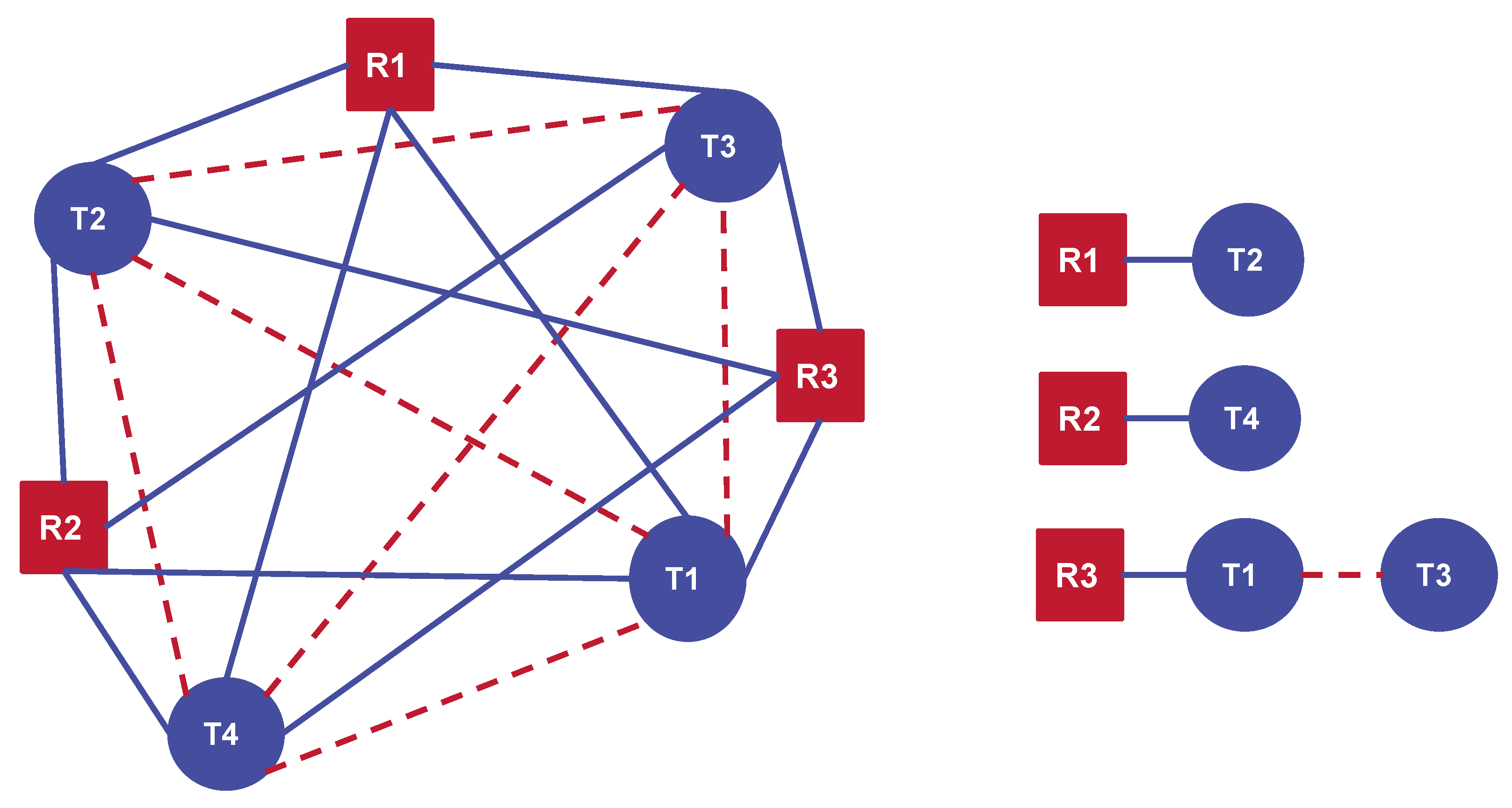
The MRR-MM problem is defined as: To allocate a set of ordered tasks to each robot so as to minimize the maximum cost incurred by any one of the robots to sequentially execute its allocated group of ordered tasks. Our problem is illustrated in Figure 1 for a case of 3 robots and 4 tasks. The blue lines indicate the utility costs of the robots to each of the tasks. The red dashed lines are the utility costs between the tasks. Based on the utility costs, the tasks are allocated to each of the three robots in a such a way that this set and sequence of tasks minimizes the highest cost incurred by any one of the robot.
The problem can be described as:
Given:
- M is the number of robots
- N is the number of tasks ()
- Utility cost for doing each task
- Utility costs between robots-robots, tasks-tasks, and robots-tasks
Objective: Minimize the maximum cost incurred by any one of the robots (when ordering the tasks in sequence and assigned to a robot) such that,
Constraints:
- Each robot does at least one task.
- Each robot can have different start locations (multiple depots).
- The robots are not required to return to their starting locations (depots) after the task completion.
- The utility costs are asymmetric (the cost between two points A → B is not the same as between B → A).
- The utility costs need not obey triangle inequality.
2.2. Problem Name
The MRR-MM problem has over the years been given different names by different researchers. For example, Parker [25], who was the first to address this problem, named it the Alliance Efficiency Problem (AEP), and Lagoudakis [21] named it the Multi-Robot Routing problem. Most recently, Turpin [26] named it the Minimum Maximum Multiple Depot Vehicle Routing Problem (MMMDVRP). The problem can also be called as Min–Max Multiple Depot multiple Asymmetric Traveling Salesman Problem (MMMDmATSP), or Asymmetric Bottleneck multiple Traveling Salesman Problem (ABmTSP) [27]. However, throughout this paper, the term “Multi-Robot Routing problem with min–max objective” (MRR-MM) will be used for this problem.
2.3. Assumptions
In practical case, the number of tasks N should be much larger than the number of robots M. The task allocation is done based on two costs. First, the “utility cost”, which can be considered as the path length or the time taken by the robot (transit cost) to move between two consecutive tasks. Secondly, the “utility cost” for doing a single task. This utility cost is very important for robots involved in warehouse or mobile manipulator robots and hence it is considered here. All robots have identical capabilities and can do any of the available tasks. The problem allows asymmetric utility costs. So, the utility costs need not obey the triangle inequality. The transit costs between tasks depend on the order. The starting points of the robots may or may not be different for the robots (multiple depots). It is also not required for a robot to return to its start position after completing the tasks (open tours). It should be noted that the problem does not focus on the scheduling of tasks to each robot, i.e., the time at which the task is done. Instead, it focuses on the sequential ordering of tasks and their assignment to each robot based on the utility costs between the tasks. The temporal constraint as waiting times, arrival times, etc. can also be added to the utility costs but the problem formulation does not deal with the time schedule for the robots.
In case of real-world robotics scenario, we consider the environment similar to that of an automated warehouse. The communication bandwidth issues or map uncertainties are ignored and, hence, it is assumed that all information is available to all robots at all times. The acceleration-deceleration of the robots are also not considered in our study assuming the robots move with a constant velocity. This work’s main focus is on finding initial optimal paths for all the robots. The optimal paths are subjected to change when the robots’ paths conflict with each other causing collision (this work is a part of an upcoming paper). In our paper, we assume the robots follow traffic rules [28] or prioritization [29] to avoid this collision. The number of robots and tasks used in the experiments are taken from a typical warehouse data [30].
2.4. Problem Classification
There are several taxonomies to classify variants of MRTA problems [31,32,33]. The taxonomies do not contradict each other, but provide additional information on the problem category. According to Gerkey [31,34], MRR-MM problem can be classified as Single robot Tasks-Single task Robots-Time-extended Assignment (ST-SR-TA) problem. Though most ST-SR-TA problems can be treated as Single robot Tasks-Single task Robots-Instantaneous Assignment (ST-SR-IA) problems with a time-extended schedule, our problem cannot be treated as one. The MRR-MM problem is harder than ST-SR-TA as the objective deals with allocating a group of tasks sequentially to the robots. However, our problem can also be treated as an unweighted scheduling problem at every time instant according to Brucker’s terminology [35].
According to Korsah et al.’s iTax taxonomy [32], our problem can be classified as In-Schedule Dependencies ID (ST-SR-TA). This is because the robot-task assignment depends on other robots and tasks (intra-schedule dependencies) when the main objective of the problem is to minimize the maximum of the slowest robot of all the given robots.
By Nunes et al.’s taxonomy [33], this problem can be considered under ST-SR-TA:TW—Time Windows with soft temporal constraints and deterministic allocations. There is no time window constraint in this problem. However, it consists of the other two sub-problems in this category: Assignment and ordering. Moreover, when the precedence constraints are enforced in this problem, it may be categorized under ST-SR-TA:SP—Synchronization and Precedence with soft temporal constraints and deterministic allocations.
2.5. Computational Complexity
Even a simplified version of the MRR-MM problem is NP-hard. This was proved by Parker [36], who compared it to the famous Partition problem [37], which is NP-complete, and showed that it is a special case of this problem. Hence, this problem is NP-hard with the number of tasks; an optimal solution cannot be found in a reasonable time when the problem size is large and heuristic methods are required to find approximate solutions for this problem. So, Arkin et al. [38] developed a 7-approximation algorithm for this problem.
3. Related Work
In this section we review the “MRR-MM problem”, as dealt with by different research communities and more specifically the approaches by robotics community. The works listed below are also closely related to our problem but also differ from it in some factors, like symmetric costs or single depot (one start/end point for all the robots or the robots are are required to come back to this point), or the objective to minimize the sum of the total costs (not min–max), or some additional constraints like neighborhoods visitation or obeying Dubin’s path.
3.1. Research Communities
The MRR-MM problem is very important and an appealing problem to a huge number of researchers across different research communities and domains. Due to a lack of inter-disciplinary research terminology, researchers have used names in-line with their community vocabulary.
3.1.1. Operations Research
For example, some OR researchers have dealt with the variants of this problem under the umbrella terms as Multiple Depot Multiple Traveling Salesman Problem [39], Multi-Vehicle Routing Problem [40], Pick Up and Delivery Problem with open depots [41], Min–Max Multi-Depot Vehicle Routing Problem [27], Multiple Traveling Salesman Problem with min–max [10,42], etc. These problems differ with ours in terms of special constraints adapted specifically for its application. The multiple Asymmetric Traveling Salesman Problem (m-ATSP) with min–max objective [27] is similar to our problem but allows multiple depots (equally many depots as salesmen), and “nomadic” robots (i.e., the robots can end in other places than they started). Other OR researchers use a generic name and do not explicitly mention the unique constraints, using terms as Scheduling of multiple trucks [24,43], Nurse Location problem [44], Communication/Location routing problem [45], Vehicle routing problem [46], Orienteering problem [47], etc.
3.1.2. Mathematics
The Mathematics community has contributed with fast and better approximation algorithms for NP-hard and NP-complete problems of this type [48,49]. They have also worked on our problem and its variants but use different names for it. Combinatorial problems like the classical set cover problem [50], the N path cover problem [38], Generalized Assignment Problem [51], Shortest Common Super String Problem [52], Dial-a-Ride problem [53], etc., are some examples that have been widely explored. Arkin et al. [38] devised a number of approximation algorithms for different variants of the vehicle routing problems. One such problem variant was the min–max N path problem, which is similar to this problem, with the difference that the robots do not have multiple start locations. The proposed approximation algorithm had a sub-optimality bound, which guarantees that the solution will not be more than four times the optimal solution.
3.1.3. Robotics/Artificial Intelligence
MRR problems have been widely researched by the robotics community in the last decade. The terms “scheduling”, “assignment”, and “allocation” are used interchangeably. “Assignment” is the term used for assigning robots to tasks (usually a one-to-one mapping or linear assignment). “Allocation” is the term used for grouping tasks together, and then assign them to one or more robots (one-to-many assignment). “Scheduling” considers the time instant at which the task allocation or assignment should be done by each robot. This leads to many name variants. Another reason is that the AI community addresses this problem from the Multi-Agent perspective and the robotics community approaches this problem from the Multi-Robot perspective. For example, Multi-robot (task) Assignment Problem for Grouped Tasks (MAP-GT) [54], Target Assignment and Path Finding (TAPF) [23], and Multi-Vehicle Multi-Goal Planning [55]. All these problems include assignment or allocation of tasks/goals to robots. Similarly, the Set-cover problems are termed as coverage planning problem of drones/robots and also termed as surveillance planning problems. For example, Faigl et al. [55] treated our problem as a Multi-Vehicle Dubin’s Traveling Salesman Problem with Neighborhoods. The authors studied the MRR-MM problem with two additional requirements: One to ensure that the task assignment respects Dubin’s curvature and one that allows the robots to visit a small neighbourhood around the tasks/goals instead of a specific task location. Another related work is by Lagoudakis et al. [21] who studied three different objectives, “min–max”, “min-sum”, and “min-avg”, and solve the problem using an auction algorithm. The main difference from our problem is that Lagoudakis et al. [21] require symmetric utility costs that obey the triangle inequality between robots and tasks. Other methods try to reduce or transform the problem into a single TSP and apply the existing exact TSP-algorithms for the same and then combine the solutions [10].
3.2. Approaches
In this section, we review all the problem formulations and methodologies that have been used for solving this particular problem.
3.2.1. Behavior-Based Models
In 1995, Parker [25] suggested the MRTA distributed architecture L-ALLIANCE, where robots learn from their experiences to schedule and estimate their utility cost. The method focused on fault-tolerance and adaptability rather than optimality or computational resources, since the major goal was a fault tolerant system that could work with fallible robots with uncertain sensors in dynamic environments. Parker designed a fully distributed, behavior-based architecture and tried to solve this problem by giving each of the robot capabilities to be fully autonomous and work in cooperation even if one or more robots failed in the team. Each robot had a behavioral set and the use of motivational behavior mechanism helped a robot choose tasks and accordingly adapt the environment and other robots. Later, a learning mechanism was implemented for this architecture [36], whereby the robots could learn from experiences. It was claimed that if “L-ALLIANCE” was well-trained, it could outperform the greedy approach but it was not guaranteed to find the optimal solution.
3.2.2. Combinatorial Optimization
As mentioned before, Faigl et al. [55] treated this as a multiple Dubin’s Traveling Salesman Problem with Neighbourhoods (m-DTSPN). The problem was specifically designed for the [56] MBZIR competition, where three UAVs (Unmanned Aerial Vehicles) had to visit 22 targets so that the cost of the slowest UAV was minimized. The UAVs generally require smooth trajectories so that the low-level trajectory controller can follow the path, and so the Dubin’s model was introduced. Moreover, the UAVs were required to only reach the neighbourhood of the targets to capture the target, so a Variable Neighbourhood Search method along with Self-Organizing Maps were used. The objective was to quickly get satisfiable solutions and did not, therefore, focus on the computationally demanding optimal solutions. A simple implementation of this method for our problem case is to introduce “k-means clustering” of the group of tasks and use a TSP solver for each cluster.
3.2.3. Auction-Bidding Algorithm
The auction-based coordination method by Lagoudakis et al. [21] is a system where all the robots are bidders and the targets/goals are goods. In each round of bidding, the robots exchange their bids with each other and each one of them compute the lowest bidder locally and in parallel. By doing so, there is a decentralized task allocation for the robots. Moreover, the selection of bids and the cost computation determine the quality of the solution. The algorithm then used insertion heuristics for each local group to quickly find solutions, which also meant non-optimal solutions. The method requires symmetric costs between robots and tasks, which cuts the search space in half. The paper presents the theoretical analysis of the auction method and its application to small size problems but no real-world experiments were conducted.
3.2.4. Graph Theory
In this formulation, an undirected graph is constructed (either in a stochastic or deterministic manner), where the robots and tasks are vertices on the graph and the edges are the utility costs connecting these vertices. This becomes a multi-digraph (or directed multi-graph) with asymmetric costs. The problem is considered to be solved if one can find M discrete edges (one for each robot), starting with the robot vertices and connecting some tasks’ vertices in sequential order such that the cost of the slowest robot edge is minimized. So, there are possible assignments, and for each assignment the minimum cost Hamiltonian path with permutations needs to be found. Turpin et al. [26] approached this problem using a very fast approximation algorithm that produced near-optimal and complete solutions. The algorithm first found the minimum spanning forest for all the task vertices and sought to find an approximate Hamiltonian path, which was then divided into M sequence paths. A set of refinements and heuristics were applied to reorder the tasks as well as to make sure the cost was not more than five times the optimal solution obtained from [38]. This is the only work that directly approaches the MRR-MM problem as us and so we will use it for comparison in Section 6.
As seen from this section, the same problem has been formulated differently by various research communities and also been studied differently. However, there is a lack of common terminology between these communities and the problem is given different names. This indicates that any NP-hard problem should be studied across different research communities and a concise interdisciplinary terminology is needed to study and track the literature, which is part of an upcoming paper. We now introduce our unique problem formulation of the MRR-MM problem in the next section.
4. Permutation Matrix Approach
The Hungarian algorithm [57] is the fastest method for finding optimal solutions in a linear assignment (one-to-one) problem [58]. The algorithm seeks to find the assignment of tasks to the robots such that: (a) The total cost of the assignment is minimized, (b) each task is assigned to one robot and (c) each robot is assigned to one task. The algorithm expresses the problem in the form of a matrix, say, a non-negative cost matrix (the matrix element is the cost of assigning j to i). The minimum cost is then found by permuting the rows and columns so that the trace of is minimized.
where and are permutation matrices.
The permutation matrix approach for the MRR problem can be viewed as a generalization of these ideas to our problem, i.e., when the assignment becomes one-to-many, and the ordering of many tasks is also considered (as in case of our problem), how can the matrix be formulated for this type of problem?
Given, M robots and N tasks with a utility cost matrix (cost between tasks) and task vector (cost for doing a task), we define a solution matrix , of size , with binary variables:
For an example with two robots (A and B) and three tasks (, and c), the complete set of tasks is , where S and E followed by the robot letter are the start and end positions of the corresponding robot respectively. The matrix is then of size :
The element is read as “the task a is followed by task b”. In this matrix, there are many undesired transfers and first order loops (doing the same tasks again i.e., the diagonal elements) that can be avoided by fixing their corresponding matrix elements to zero, and the effective transfer assignment matrix looks like this:
This effective matrix can have 120 permutation matrices (the permutation matrices are the extreme points of the set of doubly stochastic matrices). Which is the solution space of our problem. For example, one solution is,
This corresponds to (first robot task allocation) and (second robot task allocation), which is read as “the robot A goes from start position, does
task b and then goes to end position A”, and “the robot B goes from start position, does
task a followed by task c, and then goes to end position B”.
Our problem is now encoded in a matrix form and the search space is the list of all permutation matrices of the given size (for our example, it is 120). Then, the optimal solution to our problem is the valid permutation matrix with the minimum cost. Valid matrices do not have any loops. Loops route the robots to an already done task. In our example above, with a sub-matrix, there are 120 permutation matrices, of which 24 are valid matrices without any loops. The validity of a solution matrix can be found by calculating the propagator [59] of the permutation matrix. Minimum cost matrix is the permutation cost with the minimum transport cost. The cost of the solution matrix can be found by using the values of the solution matrix applied on the utility cost matrix and task vector , similar to the manner used in the Hungarian algorithm [57]. Or, we can also compute the transport cost using a design variable (explained later).
One can use any search method to find this “valid and minimum cost” permutation matrix, i.e., the optimal solution matrix. In our paper, we use two methods—Deterministic Annealing (DA) method [60] and Simulated Annealing (SA) [61] to search for this solution matrix. We later compare the results with the heuristic method in Section 6.
5. Methods
In this section, we briefly explain the three methods—SA, DA and Heuristic used to solve this problem before conducting experiments.
5.1. Simulated Annealing
SA is an iterative method that begins the search with a random valid solution, say . This solution is then compared with another random solution in the neighbourhood and the system probabilistically decides about moving between the two solutions. This step is repeated until a given computation budget is exhausted. The SA method gives optimal solutions within few seconds for small problem sizes (n lesser than 20). However, for n > 10, the solution quality converges to global minima only as the time goes to infinity, i.e., asymptotically optimal. If the computational time is higher, the solutions get better.
5.2. Deterministic Annealing
Deterministic annealing [60] is based on applying the mean-field concept on the “Potts-spin model” with an annealing period [62]. To begin with, a Potts-spin doubly stochastic matrix (size same as ) is initialized with small random values. Every element of the matrix is then updated according to an objective function termed as the local field . This local field consists of: term which enforces a minimum make-span, the term which imposes a penalty for solutions with loops, and the term which dampens oscillations in the system. After every update of the matrix, the matrix is normalized using the Sinkhorn normalisation [63] to maintain the matrix to be doubly stochastic. Depending upon the computational budget and the parameters of the objective function, the system eventually converges to a global minimum. Every element in the matrix is updated according to the equation
where, is the annealing temperature and the local field are the values of the matrix,
where, is the Propagator matrix given by,
is the maximum value of the vector given by
and is the maximum value of the vector given by,
and are the weighing factors for the loop and stabilisation functions respectively (the details of this method is given in an upcoming paper).
5.3. Heuristic Graph Search
A simpler method, inspired by Turpin et al.’s work, is devised for this work. In a graph G, the robot vertices are ignored and the shortest path connecting all the task vertices (shortest Hamiltonian path) is found. The problem of finding whether a given graph has a Hamiltonian path or not is a NP-hard problem. In case of a non-existent edge between certain tasks, then an infinite cost value can be assigned between those tasks. The process is also called edge evaluation. The problem of finding the shortest Hamiltonian path is similar to the TSP. There are many algorithms available for solving instances of tens and thousands of vertices in a TSP and hence, this can be computed. After obtaining the shortest Hamiltonian path (connecting the tasks), it is then cut into M number of chunks, based on the average chunk length or the largest edge costs present in this path. Now, the problem is reduced to a simple linear assignment problem between the M robot vertices and M chunks (sequences of tasks). Each sequence chunk’s first and the last task vertex is assigned to one of the robots by using the Hungarian algorithm. The solution quality highly depends on how the overall Hamiltonian path is cut in the right places. Turpin et al. [26] in their paper did a number of pruning steps to get the right “cut” for obtaining very fast and good quality solutions.
6. Experiments and Results
6.1. Datasets
In this section, we solve the MRR-MM problem using the three different methods and study their results. However, before setting up the experiments, the data for the utility cost matrix and the task vector that will be used for the experiments must be generated. We create four different datasets for the matrix. The vector is generally assumed to be 1, i.e., the cost for doing a task is always 1 (for all tasks). Data are generated for varying problem sizes, from (, ) to (, ).
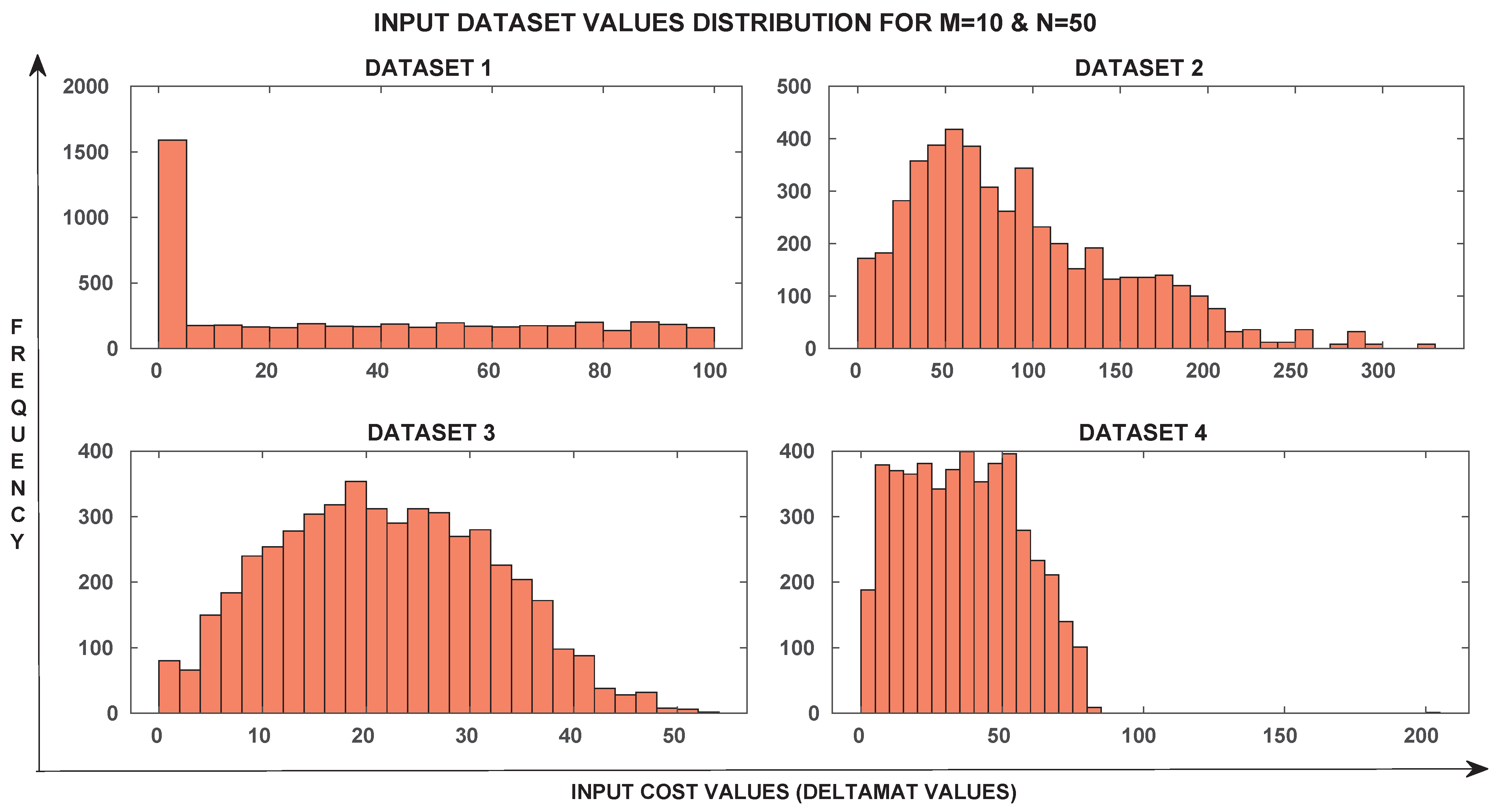
In dataset 1, random values for are drawn from a uniform distribution. The dataset 2 consists of random positions that are considered to be the pose of robots and tasks. The Euclidean distances between these poses form the matrix for the dataset 2 which is a normal distribution. For datasets 3 and 4, we make use of 12 occupancy grid maps. Ignoring the outliers, the Figure 2 shows the distributions of the utility cost values in the four datasets. Experiments were conducted on the four different datasets to solve the MRR-MM problem using SA, DA and the heuristic search methods. All the three algorithms (https://github.com/jenniferdavid/taskallocation/tree/master/potts, accessed on 9 November 2021) were implemented using C++ with Eigen library and Matlab running on Ubuntu 16.04 with octa-core Intel i7 processor and 15.6 GB memory.
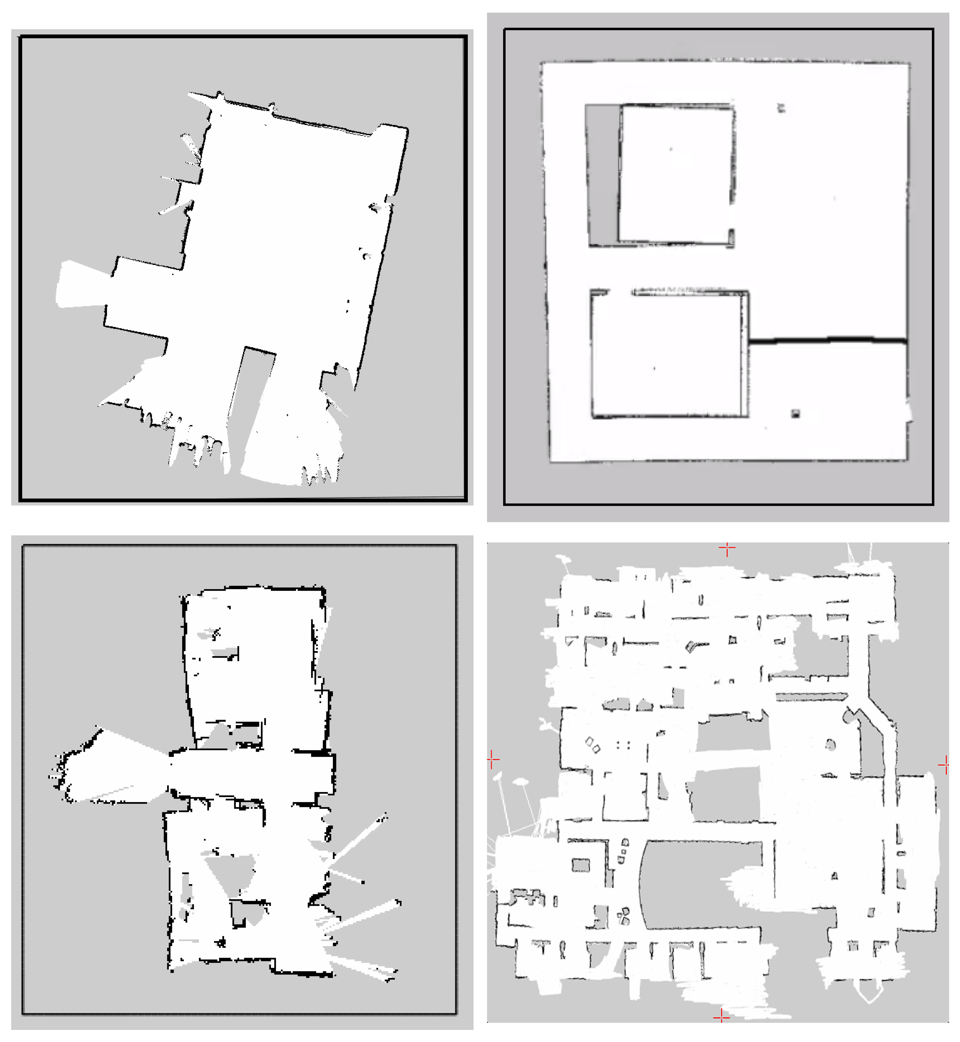
Figure 3 shows the maps used for dataset 3 and 4 that are generated using Gmapping [64] from ROS packages, simulated worlds and in real world. For dataset 3, the utility costs are the spatial Euclidean distances between the robots and tasks (similar to dataset 2) but on the given static map. In each of these maps, random obstacle-free positions are chosen as the pose of tasks and robots. Obstacles in the map are ignored and each map has a different resolution. This dataset is a normal distribution and this simulation is only done for task allocation purpose as the robots’ motion cannot be executed due to the presence of obstacles in the map. The dataset 4 considers the utility costs to be the actual path length cost between the robots and tasks in the same set of 12 occupancy grid maps as used for the third dataset. Random positions are chosen as the pose of tasks and robots and the path length between them is computed using an A* path planner [65]. This dataset is also a normal distribution. After the task allocation is calculated, the robots execute the motion in the given map environment, navigating with obstacles.
6.2. Scalability Comparison—Optimality and Computing Time
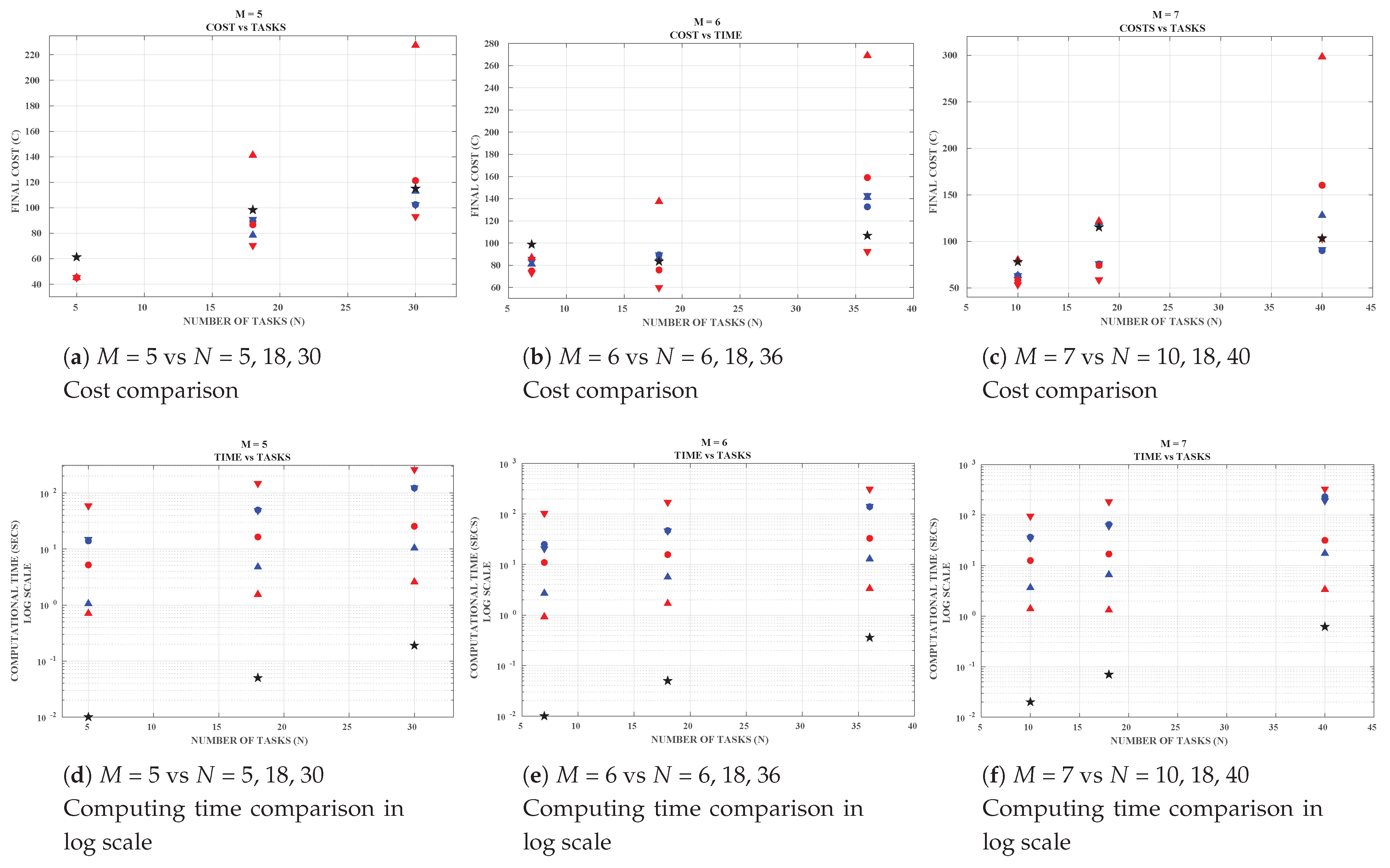
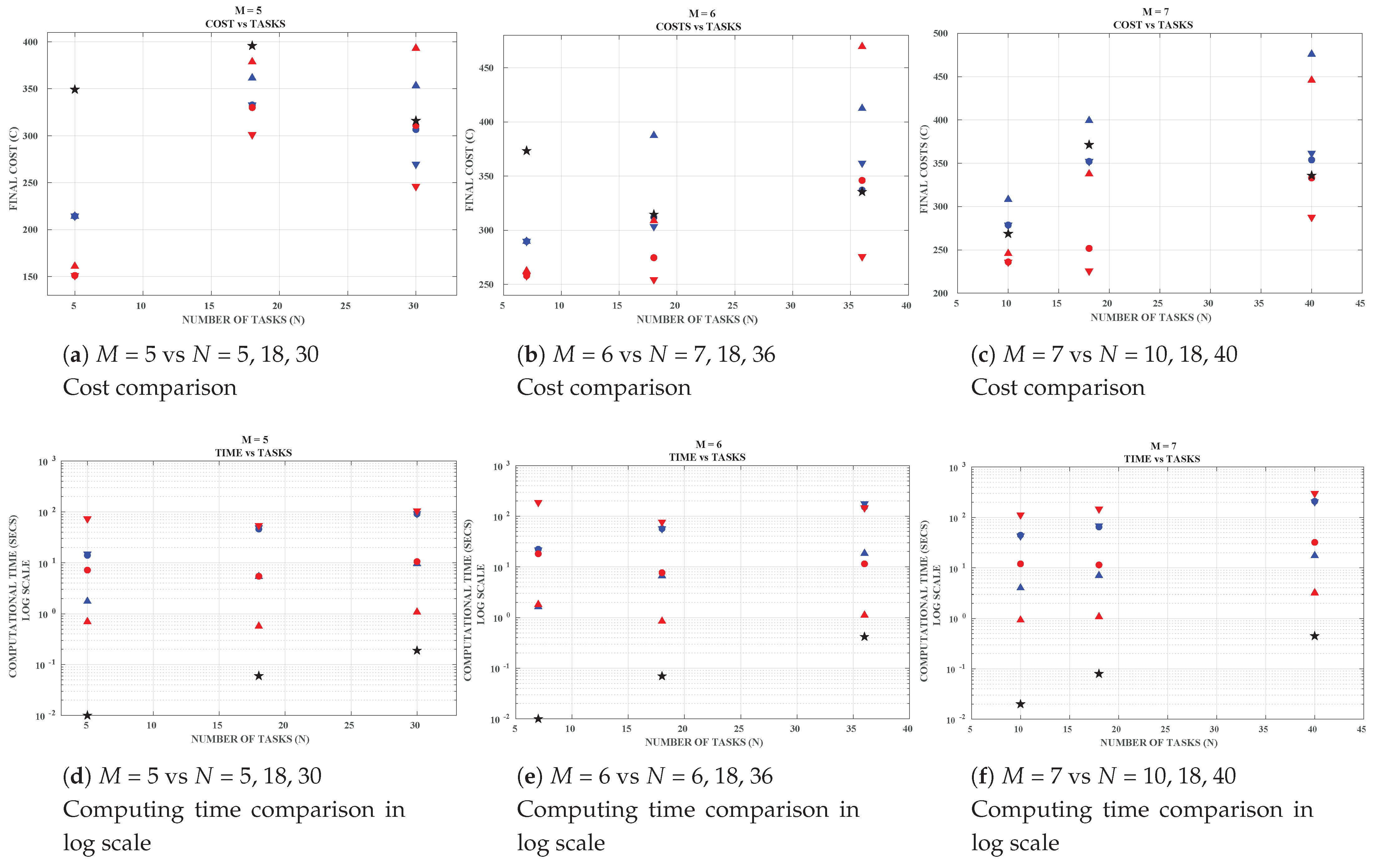
A comparison study was conducted on the scalability of these approaches in terms of best cost and computation time for each of the four datasets. Three experiments were conducted for different numbers of robots and tasks. In each experiment, the number of robots (M) was kept constant and the number of tasks (N) varied. In the first experiment, and . In the second experiment, and . In the third experiment and . The SA and DA methods were run at an annealing rate of 0.9, 0.99 and 0.999 respectively for each of the three experiments. The weighing factors for DA and were set to 1. Each combination of N and M was repeated six times, and the results reported below are the median values of these six repeats.
The results on dataset 1, with uniformly distributed values in the matrix, are shown in Figure 4. From the figure, it can be observed that the SA at 0.999 yields very good solutions and SA at 0.9 gave poor results. This is because of the longer annealing time which gives enough time for better solution convergence. However, the computation time is large for SA at 0.999 compared to SA at 0.9 due to the long running time. As expected, the heuristic method has the shortest computation time but the solution costs are not satisfactory. Similar results are obtained for dataset 2 as well which is shown in Figure 5 for both SA and heuristic.
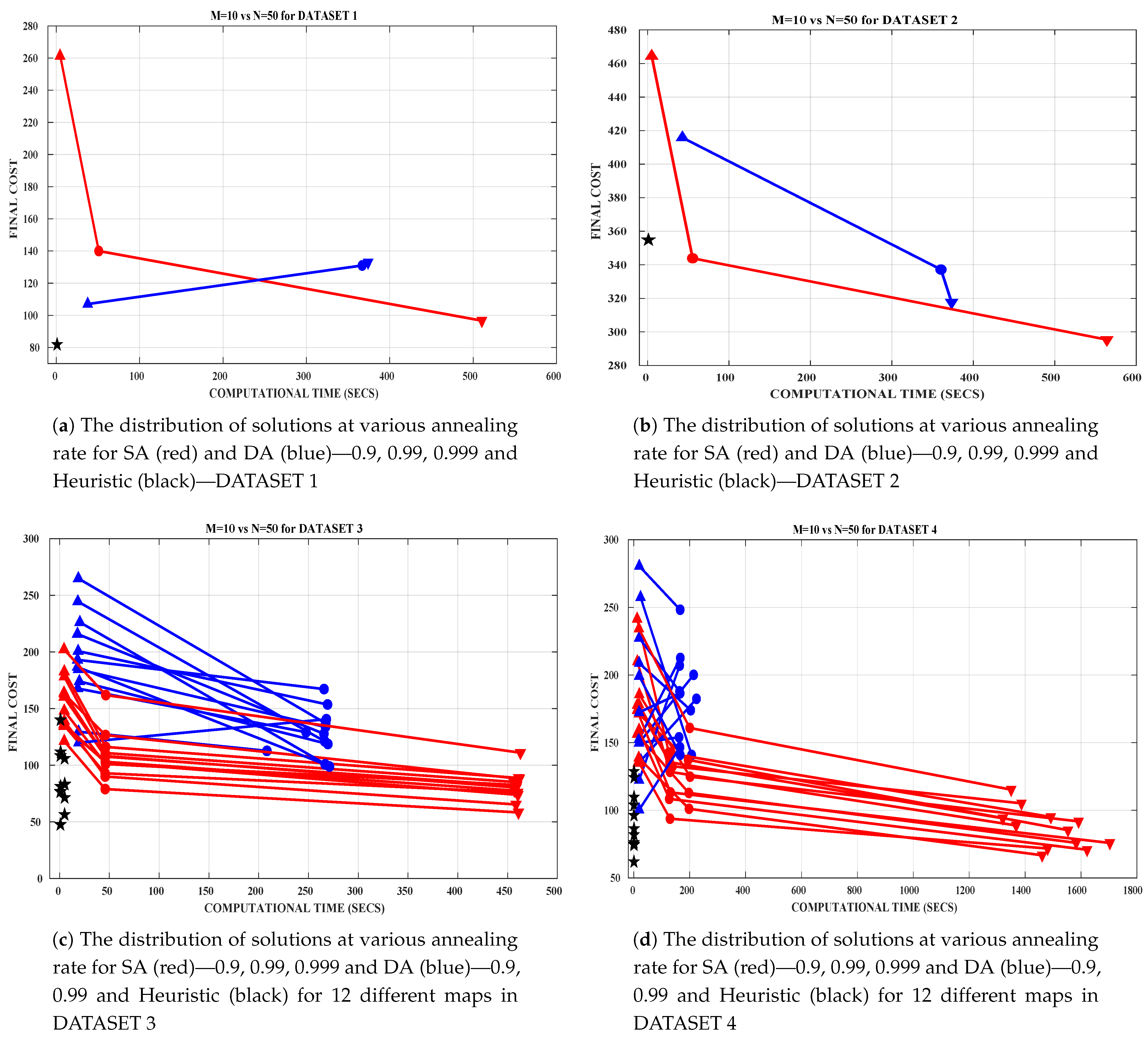
The DA method is able to produce comparatively good quality solutions in a considerable amount of time for dataset 1. However, for dataset 2, the solution quality of DA method deteriorates and performs poorer than SA at 0.99. The only difference between both the datasets is that the dataset 2 is generated from a normal distribution compared to the dataset 1 generated from uniform distribution. Experiments conducted for a size of M = 10 and N = 50 for all the four datasets is shown in Figure 6. In this case, SA is run at 0.9, 0.99 and 0.999 and DA at 0.9 and 0.99 respectively. These plots clearly show that the heuristic method is faster and produces good quality solutions in most of the cases (not all). The SA method produces good quality solutions at 0.999 but with higher computing time. The performance of DA method is good as compared to other methods but only with dataset 1. For the other datasets, the solution quality is poor for the DA method. In this case, SA at 0.99 is a better choice that has a proper trade off between both the parameters. These results show that the optimal choice of algorithm depends on the dataset size and the computational resources.
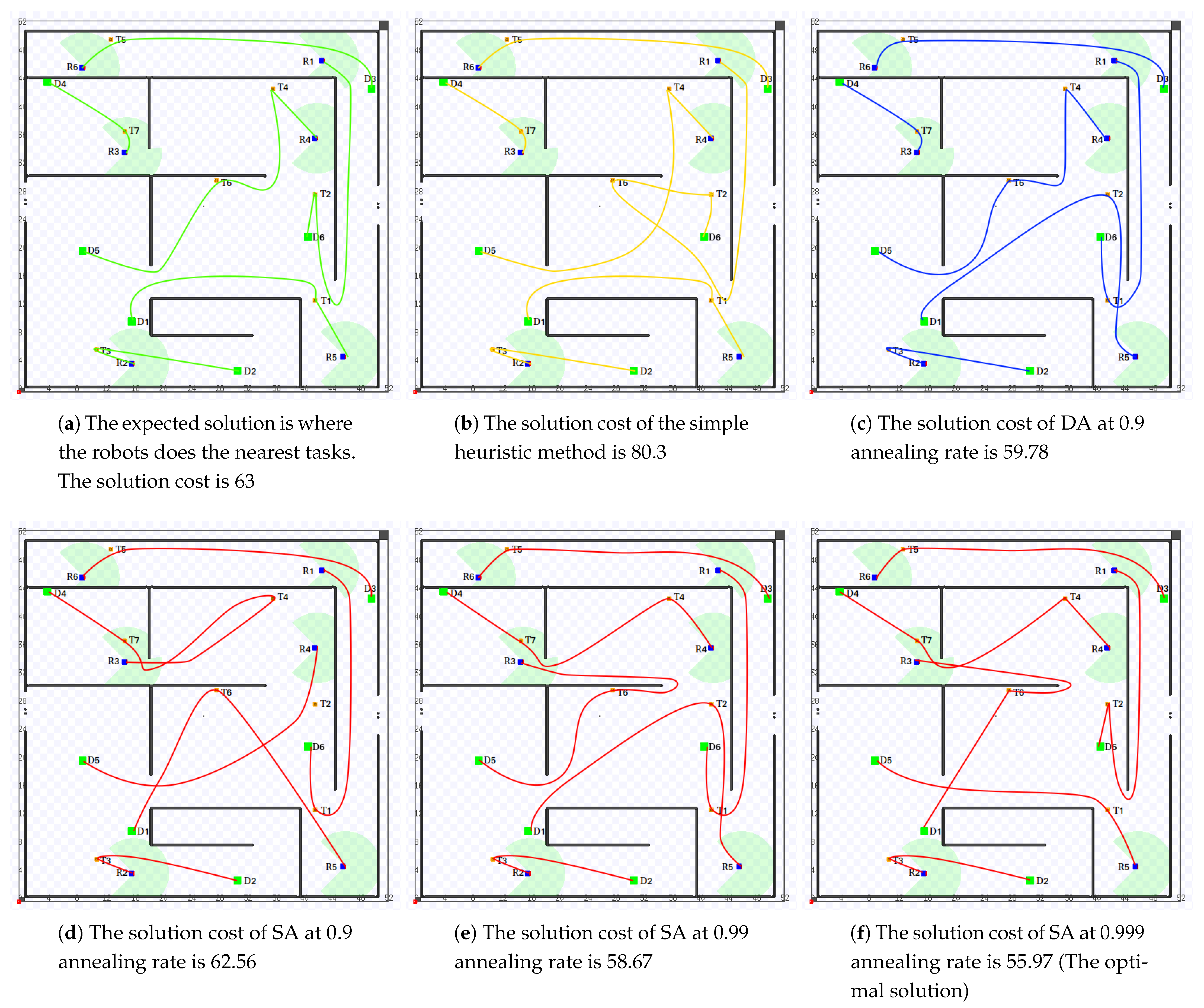
6.3. Motion Execution
For dataset 4 the values are the actual path lengths computed from the occupancy grid maps. In this case, the robots’ motions can be executed to visualize the assignment and ordering of different tasks with respect to the robots. The simulation was conducted on differential-drive robots on a 2.5 simulator Stage (https://youtu.be/gXSRuJjHJDM, accessed on 9 November 2021) and ROS. One such visualization is shown in Figure 7 for M = 6 and N = 7. The robots are shown in blue, the tasks are marked orange, and the final drop off points are green. A “quick and simple” routing solution is to group each tasks to the nearest robot. This is shown in Figure 7a and gives a cost of 63. However, in this case, though the heuristic method produces faster solution cost of 80.3 in 5.2 s compared to other methods, the DA gives a better solution of 59.78 in 20.2 s. As expected, SA at 0.999 gives the optimal solution of 55.97 at 1033.57 s. From this experiment, it could also be seen that the expected solution need not be the optimal solution always.
6.4. Algorithmic Efficiency and Completeness
It should also be noted that SA is an anytime algorithm. One can stop the algorithm anytime during the annealing and have a valid solution. In contrast, both the Heuristic method and DA require a time frame to converge to a solution. The quality of the SA solution highly depends on the annealing rate. Both DA and heuristic algorithms run to completion, i.e., the solutions are obtained only after the algorithm comes to an end.
The heuristic method finds the Hamiltonian path connecting all the tasks, which is an NP-hard problem. The DA method needs to perform a Sinkhorn normalisation to keep the updated matrices to be doubly stochastic which is the most time-consuming part of the algorithm. Moreover, it also needs an annealing period for the solutions to converge to the global minimum.
SA always begins with an existent solution. The annealing period plays a vital role to find whether a solution exists or not for both SA and DA. The heuristic method, however, always returns a non-existent solution if no possible solution exists.
Solution Space
The solution space of this NP-hard problem exhibits factorial growth with the number of robots M and the number of tasks N, as shown in Table 1.
This can be explained as follows. For any pair of N and M the total number of solution matrices is given by,
The total number of valid solutions (matrices without loops) is,
The number of matrices with loops is
7. Discussion
In this section, we discuss the permutation matrix formulation in detail and how to extend this formulation to other variants of the problem.
7.1. Distributed Variant
This problem formulation is a centralized task allocation method that focuses on the global optimal solution. It assumes that all the robots and tasks are available, and are known at all times and there is no communication issues in the system. The heuristic method also has the same assumptions. However, the centralized approach is not feasible for practical purposes. Hence, a distributed variant of this problem is required for a number of reasons. In real world scenarios, due to uncertainties, it is not possible to have an accurate utility cost matrix between the robots and tasks, especially for big problem sizes. More than the global optimal solution, one has to focus on the computing time, replanning and communication issues in such cases. So, the distributed variant of the problem is constructed by breaking down the problem into smaller sub-problems. The robots and tasks are first grouped based on a heuristic or k-means clustering and then the matrix and are updated accordingly. This variant is useful in a scenario when one of the robots breaks down or is not available for task execution after the allocation is completed. If the problem is divided into sub-problems, then it is easy to address the robot breakdown by solving that specific sub-problem again. The distributed variant will also be useful in a case, when all the resources are not required to be used, i.e., the minimum number of robots could be employed instead of using all the robots in hand. However, as with any approach, distributed variant leads to sub-optimal solutions.
7.2. Other Variants
7.2.1. The Delta Matrices
In case of scenario like the scheduling of trucks in a container terminal [24], there are many other variables involved apart from the utility cost. It could be the arrival time of the trucks/robots, the waiting times for the robots, etc. In such a case, a proper pre-processing of these values is required to create a realistic utility matrix that captures the essence of the problem. For example, in Equation (4), some of the unwanted task orders are set to zero in the assignment matrix . This is typically enforcing constraints on our problem formulation. Another way of implementing these constraints would be to set high cost for such task orders in the utility matrix and so are ignored during the minimum cost search. This shows that we can also enforce other constraints on the problem depending upon the requirement.
7.2.2. Precedence Constraints
In our problem formulation, there is no specific precedence ordering constraints on the tasks, i.e., “task ‘b’ SHOULD be done after task ‘a’”. The solution is obtained by ordering any tasks after any other tasks. However, when we are given a predefined set of task precedence orders, this constraint can be implemented in the problem formulation, by setting the corresponding utility costs to large values. In case of our example, in a predefined task order case of 3 tasks, say as in, “task ‘a’ should be done before task ‘b’ which should be done before task ‘c’”, the lower diagonal of the utility cost matrix can be set to a large value. This precedence constraints reduces the solution space by half. Hence, for this case, SA (0.9) outperformed DA up to problem size. Again, for bigger problem sizes, DA provided good results in terms of time and final cost.
7.2.3. Identical Utility Cost
When all the task orders are given the same values ( = a = b = = .... etc.), it violates the initial constraints that is set. For example, when = a is set, it requires to set a = which is a dummy task. Hence, this case cannot be fit into our problem formulation as it does not give a permutation matrix solution set.
On the other hand, when identical utility costs are given for all the robots ( = = = ), the DA method produces solutions in which all the robots are given equal weights for the start and end (special) tasks. This implies that when there are identical robots with uniform utility cost, any robot could be used for the start or end tasks due to the identical utility cost. If the robots are identical (i.e., same cost to start and to end) then there will be identical cost values (including the minimum value). For example, if then there are 6 possible matrices with the minimum value. The maximum number of possibly unique matrices for this case, is,
7.2.4. Linear Assignment Problem
Linear assignment problem is widely used in MRTA systems [66]. When M = N, the problem is reduced to a linear assignment problem. However, the assignment in our problem formulation is based on a different objective which is to minimize the maximum of the slowest robot. Future work will involve on reducing the present objective function to a linear assignment objective that can expand the scope of this method to more problems and its performance with the classical Hungarian algorithm.
7.2.5. Capacity Constraints
In case of multi-task system, where two or more robots are required to do the same single task, or when a robot is capable of doing two tasks at the same time, the problem formulation will change considerably and this will be a part of the future work.
8. Conclusions
In this paper, different problem formulations for the MRTA problem termed as the Multi-Robot Routing problem with min–max objective is discussed in detail. The paper highlights the importance of problem formulation and the lack of terminology across different research communities. The paper also explains a new problem formulation in detail—the permutation matrix formulation for this problem which proves to be more efficient and fast. The paper also provides a comparative study between the three different approaches SA, DA and heuristics search method with extensive experiments on real-world and simulated datasets to solve this problem. The results show that the optimal choice of algorithm depends on the dataset size, and the computational resources available.
Author Contributions
Conceptualization J.D.; methodology, J.D. and T.R.; software, J.D.; investigation, J.D. and T.R.; writing—original draft preparation, J.D.; writing—review and editing, J.D. and T.R.; supervision, T.R. All authors have read and agreed to the published version of the manuscript.
Funding
This research received no external funding.
Institutional Review Board Statement
Not applicable.
Informed Consent Statement
Not applicable.
Acknowledgments
The authors would like to thank Bo Sö for the conceptualisation of the DA method and Jari Häkkinen et al. [59] for the C++ implementation of communication routing problem (which inspired this work).
Conflicts of Interest
The authors declare no conflict of interest.
References
- Claes, D.; Oliehoek, F.; Baier, H.; Tuyls, K. Decentralised online planning for multi-robot warehouse commissioning. In Proceedings of the 16th Conference on Autonomous Agents and MultiAgent Systems, International Foundation for Autonomous Agents and Multiagent Systems, São Paulo, Brazil, 8–12 May 2017; pp. 492–500. [Google Scholar]
- Baxter, J.L.; Burke, E.; Garibaldi, J.M.; Norman, M. Multi-robot search and rescue: A potential field based approach. In Autonomous Robots and Agents; Springer: Berlin/Heidelberg, Germany, 2007; pp. 9–16. [Google Scholar]
- Burgard, W.; Moors, M.; Stachniss, C.; Schneider, F.E. Coordinated multi-robot exploration. IEEE Trans. Robot. 2005, 21, 376–386. [Google Scholar] [CrossRef] [Green Version]
- Fox, D.; Ko, J.; Konolige, K.; Limketkai, B.; Schulz, D.; Stewart, B. Distributed multirobot exploration and mapping. Proc. IEEE 2006, 94, 1325–1339. [Google Scholar] [CrossRef]
- Groth, C.; Henrich, D. Single-shot learning and scheduled execution of behaviors for a robotic manipulator. In Proceedings of the ISR/Robotik 2014, 41st International Symposium on Robotics, Munich, Germany, 2–3 June 2014; pp. 1–6. [Google Scholar]
- Lemaire, T.; Alami, R.; Lacroix, S. A distributed tasks allocation scheme in multi-UAV context. In Proceedings of the IEEE International Conference on Robotics and Automation, New Orleans, LA, USA, 26 April–1 May 2004; Volume 4, pp. 3622–3627. [Google Scholar]
- Gini, M. Multi-robot allocation of tasks with temporal and ordering constraints. In Proceedings of the Thirty-First AAAI Conference on Artificial Intelligence, San Francisco, CA, USA, 4–9 February 2017. [Google Scholar]
- Zhang, Y.; Parker, L.E. Multi-robot task scheduling. In Proceedings of the 2013 IEEE International Conference on Robotics and Automation, Karlsruhe, Germany, 6–10 May 2013; pp. 2992–2998. [Google Scholar]
- Parker, J.; Nunes, E.; Godoy, J.; Gini, M. Exploiting spatial locality and heterogeneity of agents for search and rescue teamwork. J. Field Robot. 2016, 33, 877–900. [Google Scholar] [CrossRef]
- Bektas, T. The multiple traveling salesman problem: An overview of formulations and solution procedures. Omega 2006, 34, 209–219. [Google Scholar] [CrossRef]
- McIntire, M.; Nunes, E.; Gini, M. Iterated multi-robot auctions for precedence-constrained task scheduling. In Proceedings of the 2016 International Conference on Autonomous Agents & Multiagent Systems. International Foundation for Autonomous Agents and Multiagent Systems, Singapore, 9–13 May 2016; pp. 1078–1086. [Google Scholar]
- Sarkar, C.; Paul, H.S.; Pal, A. A scalable multi-robot task allocation algorithm. In Proceedings of the 2018 IEEE International Conference on Robotics and Automation ICRA, Brisbane, QLD, Australia, 21–25 May 2018; pp. 1–9. [Google Scholar]
- Gombolay, M.; Wilcox, R.; Shah, J. Fast Scheduling of Multi-Robot Teams with Temporospatial Constraints. In Proceedings of the Robotics: Science and Systems IX, Berlin, Germany, 24–28 June 2013. [Google Scholar]
- Clausen, J. Branch and Bound Algorithms-Principles and Examples; Department of Computer Science, University of Copenhagen: Copenhagen, Denmark, 1999. [Google Scholar]
- Liu, C.; Kroll, A. A centralized multi-robot task allocation for industrial plant inspection by using a* and genetic algorithms. In Proceedings of the International Conference on Artificial Intelligence and Soft Computing, Zakopane, Poland, 29 April–3 May 2012; pp. 466–474. [Google Scholar]
- Wang, J.; Gu, Y.; Li, X. Multi-robot task allocation based on ant colony algorithm. J. Comput. 2012, 7, 2160–2167. [Google Scholar] [CrossRef]
- Li, X.; Ma, H.x. Particle swarm optimization based multi-robot task allocation using wireless sensor network. In Proceedings of the 2008 International Conference on Information and Automation, Changsha, China, 20–23 June 2008; pp. 1300–1303. [Google Scholar]
- Mosteo, A.R.; Montano, L. Simulated annealing for multi-robot hierarchical task allocation with flexible constraints and objective functions. In Proceedings of the Workshop on Network Robot Systems: Toward Intelligent Robotic Systems Integrated with Environments, IROS, Beijing, China, 9–15 October 2006. [Google Scholar]
- Mitiche, H.; Boughaci, D.; Gini, M. Efficient heuristics for a time-extended multi-robot task allocation problem. In Proceedings of the 2015 First International Conference on New Technologies of Information and Communication (NTIC), Mila, Algeria, 8–9 November 2015; pp. 1–6. [Google Scholar]
- Maheswaran, R.T.; Tambe, M.; Bowring, E.; Pearce, J.P.; Varakantham, P. Taking DCOP to the real world: Efficient complete solutions for distributed multi-event scheduling. In Proceedings of the Third International Joint Conference on Autonomous Agents and Multiagent Systems, New York, NY, USA, 23–23 July 2004; pp. 310–317. [Google Scholar]
- Lagoudakis, M.G.; Markakis, E.; Kempe, D.; Keskinocak, P.; Kleywegt, A.J.; Koenig, S.; Tovey, C.A.; Meyerson, A.; Jain, S. Auction-Based Multi-Robot Routing. Robot. Sci. Syst. 2005, 5, 343–350. [Google Scholar]
- Liu, L.; Shell, D.A.; Michael, N. From selfish auctioning to incentivized marketing. Auton. Robot. 2014, 37, 417–430. [Google Scholar] [CrossRef]
- Ma, H.; Koenig, S. Optimal target assignment and path finding for teams of agents. arXiv 2016, arXiv:1612.05693. [Google Scholar]
- Ng, W.; Mak, K.; Zhang, Y. Scheduling trucks in container terminals using a genetic algorithm. Eng. Optim. 2007, 39, 33–47. [Google Scholar] [CrossRef]
- Parker, L.E. L-ALLIANCE: A Mechanism for Adaptive Action Selection in Heterogeneous Multi-Robot Teams; Technical Report; Oak Ridge National Lab.: Oak Ridge, TN, USA, 1995.
- Turpin, M.; Michael, N.; Kumar, V. An approximation algorithm for time optimal multi-robot routing. In Algorithmic Foundations of Robotics XI; Springer: Berlin/Heidelberg, Germany, 2015; pp. 627–640. [Google Scholar]
- Franca, P.M.; Gendreau, M.; Laporte, G.; Muller, F.M. The m-Traveling Salesman Problem with Minmax Objective. Transp. Sci. JSTOR 1995, 29, 267–275. [Google Scholar] [CrossRef]
- Kato, S.; Nishiyama, S.; Takeno, J. Coordinating Mobile Robots By Applying Traffic Rules. In Proceedings of the IEEE/RSJ International Conference on Intelligent Robots and Systems, Raleigh, NC, USA, 7–10 July 1992; Volume 3, pp. 1535–1541. [Google Scholar] [CrossRef]
- Van Den Berg, J.P.; Overmars, M.H. Prioritized motion planning for multiple robots. In Proceedings of the 2005 IEEE/RSJ International Conference on Intelligent Robots and Systems ICRA 2005, Edmonton, AB, Canada, 2–6 August 2005; pp. 430–435. [Google Scholar]
- Liu, M.; Ma, H.; Li, J.; Koenig, S. Task and path planning for multi-agent pickup and delivery. In Proceedings of the International Joint Conference on Autonomous Agents and Multiagent Systems (AAMAS), Montreal, QC, Canada, 13–17 May 2019. [Google Scholar]
- Gerkey, B.P.; Matarić, M.J. A formal analysis and taxonomy of task allocation in multi-robot systems. Int. J. Robot. Res. 2004, 23, 939–954. [Google Scholar] [CrossRef] [Green Version]
- Korsah, G.A.; Stentz, A.; Dias, M.B. A comprehensive taxonomy for multi-robot task allocation. Int. J. Robot. Res. 2013, 32, 1495–1512. [Google Scholar] [CrossRef]
- Nunes, E.; Manner, M.; Mitiche, H.; Gini, M. A taxonomy for task allocation problems with temporal and ordering constraints. Robot. Auton. Syst. 2017, 90, 55–70. [Google Scholar] [CrossRef] [Green Version]
- Gerkey, B.P.; Mataric, M.J. Multi-robot task allocation: Analyzing the complexity and optimality of key architectures. In Proceedings of the 2003 IEEE International Conference on Robotics and Automation, Taipei, Taiwan, 14–19 September 2003; Volume 3, pp. 3862–3868. [Google Scholar]
- Brucker, P. Scheduling Algorithms; Springer: Berlin/Heidelberg, Germany, 2004. [Google Scholar]
- Parker, L.E. ALLIANCE: An architecture for fault tolerant multirobot cooperation. IEEE Trans. Robot. Autom. 1998, 14, 220–240. [Google Scholar] [CrossRef] [Green Version]
- Garey, M.R.; Johnson, D.S. Computers and Intractability: A Guide to the Theory of NP-Completeness (Series of Books in the Mathematical Sciences); W. H. Freeman: San Francisco, CA, USA, 1979. [Google Scholar]
- Arkin, E.M.; Hassin, R.; Levin, A. Approximations for Minimum and Min–Max Vehicle Routing Problems. J. Algorithms 2006, 59, 1–18. [Google Scholar] [CrossRef]
- Diaby, M. Linear programming formulation of the multi-depot multiple traveling salesman problem with differentiated travel costs. Travel. Salesm. Probl. Theory Appl. 2010, 2010, 257–282. [Google Scholar]
- Oberlin, P.; Rathinam, S.; Darbha, S. A transformation for a heterogeneous, multiple depot, multiple traveling salesman problem. In Proceedings of the 2009 American Control Conference, St. Louis, MO, USA, 10–12 June 2009; pp. 1292–1297. [Google Scholar]
- Naccache, S.; Côté, J.F.; Coelho, L.C. The multi-pickup and delivery problem with time windows. Eur. J. Oper. Res. 2018, 269, 353–362. [Google Scholar] [CrossRef]
- Carlsson, J.; Ge, D.; Subramaniam, A. Solving min–max multi-depot vehicle routing problem. Lect. Glob. Optim. 2009, 55, 31–46. [Google Scholar]
- Bish, E.K.; Chen, F.Y.; Leong, Y.T.; Nelson, B.L.; Ng, J.W.C.; Simchi-Levi, D. Dispatching vehicles in a mega container terminal. In Container Terminals and Cargo Systems; Springer: Berlin/Heidelberg, Germany, 2007; pp. 179–194. [Google Scholar]
- Xu, Z.; Xu, D.; Zhu, W. Approximation results for a min–max location-routing problem. Discret. Appl. Math. 2012, 160, 306–320. [Google Scholar] [CrossRef] [Green Version]
- Nace, D.; Pióro, M. Max-min fairness and its applications to routing and load-balancing in communication networks: A tutorial. IEEE Commun. Surv. Tutor. 2008, 10, 5–17. [Google Scholar] [CrossRef]
- Applegate, D.; Cook, W.; Dash, S.; Rohe, A. Solution of a min–max vehicle routing problem. INFORMS J. Comput. 2002, 14, 132–143. [Google Scholar] [CrossRef] [Green Version]
- Pěnička, R.; Faigl, J.; Váňa, P.; Saska, M. Dubins orienteering problem. IEEE Robot. Autom. Lett. 2017, 2, 1210–1217. [Google Scholar] [CrossRef]
- Xu, Z.; Rodrigues, B. A 3/2-approximation algorithm for multiple depot multiple traveling salesman problem. In Proceedings of the Scandinavian Workshop on Algorithm Theory, Bergen, Norway, 21–23 June 2010; pp. 127–138. [Google Scholar]
- Even, G.; Garg, N.; Könemann, J.; Ravi, R.; Sinha, A. Min–max tree covers of graphs. Oper. Res. Lett. 2004, 32, 309–315. [Google Scholar] [CrossRef]
- Christofides, N.; Korman, S. Note—A computational survey of methods for the set covering problem. Manag. Sci. 1975, 21, 591–599. [Google Scholar] [CrossRef] [Green Version]
- Fisher, M.L.; Jaikumar, R. A generalized assignment heuristic for vehicle routing. Networks 1981, 11, 109–124. [Google Scholar] [CrossRef]
- Turner, J.S. Approximation algorithms for the shortest common superstring problem. Inf. Comput. 1989, 83, 1–20. [Google Scholar] [CrossRef] [Green Version]
- Cordeau, J.F.; Laporte, G. The dial-a-ride problem: Models and algorithms. Ann. Oper. Res. 2007, 153, 29–46. [Google Scholar] [CrossRef]
- Luo, L.; Chakraborty, N.; Sycara, K. A distributed algorithm for constrained multi-robot task assignment for grouped tasks. J. Contrib. 2018. [Google Scholar] [CrossRef]
- Faigl, J.; Váňa, P.; Pěnička, R.; Saska, M. Unsupervised learning-based flexible framework for surveillance planning with aerial vehicles. J. Field Robot. 2019, 36, 270–301. [Google Scholar] [CrossRef] [Green Version]
- Mohamed Bin Zayed International Robotics Challenge (MBZIRC) 2017. Available online: http://www.mbzirc.com (accessed on 9 November 2021).
- Kuhn, H.W. The Hungarian method for the assignment problem. Nav. Res. Logist. Q. 1995, 2, 83–97. [Google Scholar] [CrossRef] [Green Version]
- Burkard, R.E.; Cela, E. Linear assignment problems and extensions. In Handbook of Combinatorial Optimization; Springer: Berlin/Heidelberg, Germany, 1999; pp. 75–149. [Google Scholar]
- Hakkinen, J.; Lagerholm, M.; Peterson, C.; Soderberg, B. Local routing algorithms based on Potts neural networks. IEEE Trans. Neural Netw. 2000, 11, 970–977. [Google Scholar] [CrossRef] [Green Version]
- Soderberg, B.; Jonsson, H. Deterministic annealing and nonlinear assignment. arXiv 2001, arXiv:cond-mat/0105321. [Google Scholar]
- Kirkpatrick, S.; Gelatt, C.D.; Vecchi, M.P. Optimization by simulated annealing. Science 1983, 220, 671–680. [Google Scholar] [CrossRef] [PubMed]
- Ohlsson, M.; Peterson, C.; Söderberg, B. Neural networks for optimization problems with inequality constraints: The knapsack problem. Neural Comput. 1993, 5, 331–339. [Google Scholar] [CrossRef]
- Sinkhorn, R.; Knopp, P. Concerning nonnegative matrices and doubly stochastic matrices. Pac. J. Math. 1967, 21, 343–348. [Google Scholar] [CrossRef]
- Grisetti, G.; Stachniss, C.; Burgard, W. Improved techniques for grid mapping with rao-blackwellized particle filters. IEEE Trans. Robot. 2007, 23, 34–46. [Google Scholar] [CrossRef] [Green Version]
- Hart, P.E.; Nilsson, N.J.; Raphael, B. A formal basis for the heuristic determination of minimum cost paths. IEEE Trans. Syst. Sci. Cybern. 1968, 4, 100–107. [Google Scholar] [CrossRef]
- Liu, L.; Shell, D.A. An anytime assignment algorithm: From local task swapping to global optimality. Auton. Robot. 2013, 35, 271–286. [Google Scholar] [CrossRef]
Figure 1.
The MRR with min–max objective is described pictorially at the top, where the blue lines are utility costs between robots-tasks and tasks-robots and the red dashed lines are utility costs between tasks. The expected solution is the assignment of tasks in a sequential order such that the maximum cost incurred by any one of the robots is minimized.

Figure 2.
Distribution of the utility cost values in the Delta matrices for four different datasets.
Figure 2.
Distribution of the utility cost values in the Delta matrices for four different datasets.

Figure 3.
Occupancy grid maps used for datasets 3 and 4.

Figure 4.
Dataset 1 scalability—solution cost and computing time comparison.

Figure 5.
Dataset 2 scalability—solution cost and computing time comparison ![Robotics 10 00122 i001]() .
.
 .
.
Figure 6.
Distribution of solutions for 10 robots and 50 tasks under different datasets ![Robotics 10 00122 i002]() .
.
 .
.
Figure 7.
Stage simulator world of a maze map with 6 robots (blue), 7 tasks (orange) and 6 dropoffs (green) which shows the task allocation and the path solution cost for different methods.
Figure 7.
Stage simulator world of a maze map with 6 robots (blue), 7 tasks (orange) and 6 dropoffs (green) which shows the task allocation and the path solution cost for different methods.


Table 1.
Solution space.
| M | N | Effective Matrix Size | No. of Possible Matrices | No. of Valid Matrices |
|---|---|---|---|---|
| 1 | 2 | 3 × 3 | 4 | 2 |
| 1 | 3 | 4 × 4 | 18 | 6 |
| 2 | 2 | 4 × 4 | 4 | 4 |
| 2 | 3 | 5 × 5 | 36 | 24 |
| 2 | 4 | 6 × 6 | 288 | 144 |
| 2 | 5 | 7 × 7 | 2400 | 960 |
| 3 | 3 | 6 × 6 | 36 | 36 |
| 3 | 4 | 7 × 7 | 576 | 432 |
| 4 | 5 | 9 × 9 | 14,400 | 11,520 |
| 5 | 6 | 11 × 11 | 518,400 | 432,000 |
Publisher’s Note: MDPI stays neutral with regard to jurisdictional claims in published maps and institutional affiliations. |
© 2021 by the authors. Licensee MDPI, Basel, Switzerland. This article is an open access article distributed under the terms and conditions of the Creative Commons Attribution (CC BY) license (https://creativecommons.org/licenses/by/4.0/).
Share and Cite
MDPI and ACS Style
David, J.; Rögnvaldsson, T. Multi-Robot Routing Problem with Min–Max Objective. Robotics 2021, 10, 122. https://doi.org/10.3390/robotics10040122
AMA Style
David J, Rögnvaldsson T. Multi-Robot Routing Problem with Min–Max Objective. Robotics. 2021; 10(4):122. https://doi.org/10.3390/robotics10040122
Chicago/Turabian StyleDavid, Jennifer, and Thorsteinn Rögnvaldsson. 2021. "Multi-Robot Routing Problem with Min–Max Objective" Robotics 10, no. 4: 122. https://doi.org/10.3390/robotics10040122
Note that from the first issue of 2016, this journal uses article numbers instead of page numbers. See further details here.