
COVID-19 and Excess Mortality: An Actuarial Study

1
Aon Benfield, Telecomlaan 5-7, 1831 Diegem, Belgium
2
Department of Mathematics, Faculté des Sciences, Campus de la Plaine—CP 213, Université Libre de Bruxelles, Boulevard du Triomphe ACC.2, 1050 Bruxelles, Belgium
3
ARC Centre of Excellence in Population Ageing Research (CEPAR), UNSW Sydney, 223 Anzac Pde, Kensington, NSW 2033, Australia
4
Netspar, Postbus 90153, 5000 LE Tilburg, The Netherlands
*
Author to whom correspondence should be addressed.
†
These authors contributed equally to this work.
Risks 2024, 12(4), 61; https://doi.org/10.3390/risks12040061
Submission received: 6 February 2024
/
Revised: 22 March 2024
/
Accepted: 27 March 2024
/
Published: 30 March 2024
(This article belongs to the Special Issue Extreme Events: Mortality Modelling and Insurance)
Abstract
:The study of mortality is an ever-active field of research, and new methods or combinations of methods are constantly being developed. In the actuarial domain, the study of phenomena disrupting mortality and leading to excess mortality, as in the case of COVID-19, is of great interest. Therefore, it is relevant to investigate the extent to which an epidemiological model can be integrated into an actuarial approach in the context of mortality. The aim of this project is to establish a method for the study of excess mortality due to an epidemic and to quantify these effects in the context of the insurance world to anticipate certain possible financial instabilities. We consider a case study caused by SARS-CoV-2 in Belgium during the year 2020. We propose an approach that develops an epidemiological model simulating excess mortality, and we incorporate this model into a classical approach to pricing life insurance products.
1. Introduction
The recent SARS-CoV health crisis shows clear evidence that we are not immune to pandemics and their economic effects despite medical advances and robust health systems. Indeed, the Institute and Faculty of Actuaries (2015) indicate that the 1918 Spanish flu, which was responsible for the deaths of more than 50 million people (CDC 2021), had a cost of around GBP 13 billion to insurance companies. Pandemics are also becoming more likely (Institute and Faculty of Actuaries 2015; Saunders-Hastings and Krewski 2016), see, e.g., the H2N2 flu from 1957–1958, the H3N2 1968 flu, the H1N1 flu from 2009–2010 (WHO 2021b), and, more recently, the Ebola epidemic from 2014–2016 (WHO 2021a).
The increasing frequency and severity of pandemics call for an in-depth actuarial analysis of mortality and its effect on pricing and reserving. In particular, pandemics have a heterogenous effect on populations. Indeed, certain socio-economic groups are more susceptible than others to becoming sick and dying, making basic life tables unsuitable for pricing and risk management. It becomes natural to consider a model that incorporates epidemiological insights and dependence (Feng and Garrido 2011).1
The study of mortality is an ever-active field of research, and new methods or combinations of methods are constantly being developed. In the actuarial domain, the study of phenomena disrupting mortality and leading to excess mortality, as in the case of COVID-19, is of great interest. Investigating the extent to which an epidemiological model can be integrated into an actuarial approach in the context of mortality is, hence, relevant. The aim of this project is to establish a method for the study of excess mortality due to an epidemic and to quantify these effects in the context of the insurance world to anticipate certain possible short-term financial instabilities.
In this paper, we consider the epidemic caused by the SARS-CoV-2 in Belgium during the year 2020. For this, we used the daily COVID mortality data from the national health data of Sciensano (2021). After capturing COVID-19-specific mortality using an extended version of a susceptible-infectious-recovered-death (SIRD) compartmental model from Franco (2021), we studied overall mortality using data from the Human Mortality Database (2021) and the Cairns, Blake, and Dowd model (Cairns et al. 2006). Feng et al. (2022) also used a compartmental model to study the effect of COVID-19 in order to price epidemic insurance plans to finance medical costs during infection. Contrary to their work, we focus on the effect of COVID-19 excess of death on classical pre-existing life insurance policies. We focus on older age patients in our study, as these were most affected by the pandemic from a mortality viewpoint.
Combining these two models allowed us to perform an actuarial study on two life insurance products: whole life insurance and lifetime immediate annuities. We study these products in two settings: an old contract underwritten in 2000 and a recent contract underwritten in 2019, a year before the pandemic. We calculated their expected value and variance. We observe that the variance increases more importantly for recent contracts despite the insured being younger. For older contracts with older insured users, the variance is reduced. We hypothesize that this could be due to a different distribution of mortalities in the COVID vs. no-COVID scenario. Indeed, the uncertainty would be greater for younger individuals who still have a long period remaining in the contract. However, for older individuals, the presence of COVID-19 renders the event of death more “certain”.
The remainder of this paper is structured as follows. Section 2 presents a review of the literature related to epidemiological models and aggregate mortality models. Section 3 presents the SIRD epidemiological and Cairns et al. (2006) model used for modeling mortality, and Section 4 provides a numerical estimation and illustration of the effect of COVID-19 in the valuation of insurance products. Section 5 concludes the study.
2. Literature Review
In this section, we will discuss various strands of the literature related to mortality, in particular, the cause of death, epidemilogical, and aggregate mortality models.
Since we are interested in COVID-19-specific mortality, a possible way of studying this phenomenon is by using cause-of-death mortality models. Insights about cause of death mortality and its long-term trend can be obtained, revealing the contributors to aggregate mortality. A crucial choice has to be made with regard to the potential relationship between these causes, as these models should also provide insights about aggregate mortality. The challenge is that this dependence is not observable. Indeed, upon death, it is impossible to know what would have been the potential cause of death had the individual stayed alive. Hence, a natural choice is to assume independence (see Rogers and Gard (1991); Tabeau et al. (1999); Wilmoth (1996), and recently, Boumezoued et al. (2018) and Lyu et al. (2021) for France and The Netherlands, respectively). A clear advantage of this approach is that aggregate mortality is simply obtained by adding the mortality per cause of death.
However, recent research on cause of death mortality incorporates dependence, as this yields better long-term forecasts of aggregate mortality. Examples of this are Arnold and Sherris (2013) and Arnold and Sherris (2015), who used Vector Error Correlation Models; Li and Lu (2019); Zheng and Klein (1995) and Zittersteyn and Alonso-García (2021), who used copula theory, and Li et al. (2019), who utilized clustering methods to group different causes of death. In all cases, dependence between cause-specific death is considered, and better cause removal and aggregate mortality results were obtained. Despite their richness, these models are unable to capture the particular nature of infectious diseases in the context of a pandemic since transmission and mortality have different behaviors than natural causes of death.
In order to study COVID-19, we need to move beyond classical actuarial techniques and delve into compartmental models in epidemiology. Various models have been considered for COVID-19, from susceptible-infectious-recovered (SIR) (Abou-Ismail 2020; Calafiore et al. 2020; Huang et al. 2020) to susceptible-unquarantined-quarantined-confirmed (SUQC) (Abou-Ismail 2020). These models simplify the mathematical modeling of infectious diseases, as they divide the population into different compartments, each with a different label, such as S, I, or R, depending on whether they are susceptible, infectious, or recovered, respectively. Individuals can move between compartments, and the order of the labels generally represents the transitions between compartments. For instance, SIS means susceptible-infectious-susceptible.2 These models originated at the beginning of the 20th century in the works of Kermack and McKendrick (1927) and Kermack and McKendrick (1932) and rely on ordinary differential equations (ODE).
The susceptible-infectious-recovered (SIR) model is the basic building block of compartmental models (Hethcote 2000; Tang et al. 2020). It has been widely used in the context of COVID-19 (see, e.g., Abou-Ismail (2020); Huang et al. (2020); Tang et al. (2020); and Calafiore et al. (2020)). Italy extended this model to include the initial number of susceptible individuals and the relative factor between positive cases and the real number of infected individuals as a model parameter. Another possible extension is to consider susceptible-exposed-infectious-recovered (SEIR) models. By including the compartment “exposed”, we are able to include the incubation period of the sickness (Abou-Ismail 2020; Tang et al. 2020). The SIR and SEIR models disregard births and deaths, implicitly assuming that births and deaths have a negligible impact on the them. More complex models can overcome this (Hethcote 2000).
We are interested in analyzing excess mortality, as well as the impact of the pandemic on the life table. Ultimately, the goal is to assess the effect of COVID-19 on pricing and reserving. Hence, there is a need to move beyond the SIR model to add at least a compartment related to death. Fernández-Villaverde and Jones (2022) estimated the SIRD model for various countries, states, and cities in the context of COVID-19. Our model will be based on the SIRD compartmental design with the addition of age stratification, as suggested by Balabdaoui and Mohr (2020). Note that more complex models do include quarantine and lockdown dynamics, such as the SUQC models described above (Abou-Ismail 2020). However, we have abstracted from the SEIR or SUQC models, as our data are unable to sustain a model with the exposed (E), unquarantined (U), and quarantined (Q) compartments. Furthermore, SUQC models have mostly been used in China (Zhao and Chen 2020), where there are stricter quarantine rules that vastly differ from those used in most Western countries. Moreover, these models are of less interest within the context of insurance, as there are no cash-flow payments in cases of exposure or quarantine.
Ultimately, after studying the COVID-19 mortality dynamics, we are interested in incorporating them into a classical life table, using insights from single-population mortality models. The goal is to assess the effect of COVID-19 on products sold to individuals over 50 years old, as the effect of COVID-19 was the highest for this age segment. Hence, we choose to model aggregate mortality using a Cairns, Blake, and Dowd (CBD) (Cairns et al. 2006) model, which is fitted to Belgian historical mortality using data from the Human Mortality Database (2021). We used this model because it is considered suitable for modeling higher ages and has a simple structure with fewer parameters. Indeed, empirical analysis shows that changes in mortality rate are imperfectly correlated, supporting the use of the CBD model.
3. Methodology
In this section, we show the theoretical framework for the epidemiological model, aggregate mortality, and their integration. The products and indeces studied to assess the effect of COVID-19 are also presented.
3.1. SIRD Model
We studied the age-stratified susceptible-infectious-recovered-death (SIRD) model, as proposed by Balabdaoui and Mohr (2020). Given the differing mortality and recovery rates of infected individuals among different age groups, we incorporate age stratification into the following age categories:
- Category 1: Individuals aged 0–24 years;
- Category 2: Individuals aged 25–44 years;
- Category 3: Individuals aged 45–64 years;
- Category 4: Individuals aged 65–74 years;
- Category 5: Individuals aged 75–84 years;
- Category 6: Individuals aged 85+ years.
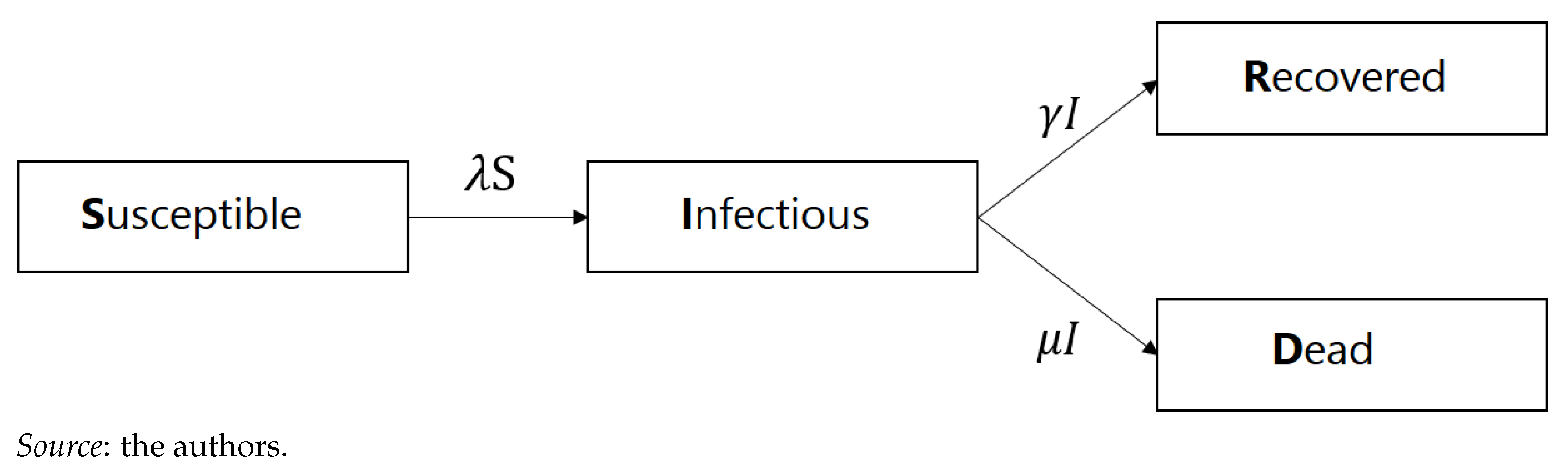
The SIRD model is depicted graphically in Figure 1.
By integrating the age component into the SIRD model and denoting the age group as “i”, we obtained the following ODE system (1) (with ):
The rate represents the transmission rate of the infection for group i, whereas and represent the mortality and recovery rates of group i, respectively. Clearly, the system (1) indicates that a person leaves the "susceptible" compartment if infected, enters into the "infectious" state when infected, and leaves either when they recover or die. A peron enters the "recovery" state according to intensity, , and does not leave this compartment.3 Similarly, a person enters the "dead absorbant" compartment according to intensity . The total population in group i is given by
Matrix C represents social contacts between the different age categories. It is important to note that we studied the epidemic over a short period, making the transitions between age categories redundant. The initial conditions of the ODE system (1) are given by
Alternatively, we can represent the ODE system (1) for all age groups in matrix form as follows:
where
The reproduction rate, , which is used to analyze the impulse of the pandemic, can be calculated as the maximum eigenvalue from the “next-generation” matrix (Franco 2021), resulting in (4)
Model Identification
The SIRD model defined by the ODE system (1) is solved by using multistep methods, as described in Hindmarsh (1983). Numerical multistep methods start with an initial point and start moving forward. These methods use past points and their derivatives in order to gain efficiency (Hindmarsh 1983).4 By applying this method to (1), we obtain the number of people in each compartment, including the main compartment of interest: , which represents the number of deaths. It does so for every time step, t, which is equal to 1 day in our case.
According to the solution of the ODE system , the number of deaths allows one to find the empirical mortality rate per age category by using maximum likelihood arguments (5):
where , , and are the central mortality rate, number of deaths, and exposure to risk for year and age category , respectively. The exposure to risk for age category i is estimated using for the global population as follows:
where and correspond to the first and last age belonging to i.
3.2. Cairns, Blake, and Dowd Model
We used the work of Cairns et al. (2006) to model global mortality and its long-term trend for old age, as this is the age category that has been most affected by COVID-19. The model is presented as a logistic regression (7):
where
- (intercept) represents the global mortality trend and is generally a decreasing parameter since it improves over time.
- (slope) represents the improvements in mortality and, typically, has a positive slope, indicating that improvements are greater during the first part of the age period considered.
We assume that the force of mortality is constant within each square of the Lexis diagram:
This allows one to obtain the equivalence between the force of mortality, , and the central mortality rate, . Hence, under Equation (8), the mortality rate, , obtained in Equation (5) corresponds to the COVID-19-related force of mortality .
We worked within a Poisson framework, with for given by (9):
This yields the following log likelihood:
where should be replaced by (9). The model is solved by using the R package StMoMo (Villegas et al. 2018).5 Goodness of fit is assessed through Pearson residuals, which should ideally have no trend. These are calculated as
Finally, projection is performed, whereby the two stochastic processes and are modeled through bi-variate random work with drift:
where and correspond to the drift, and are independent bi-variate and normally distributed parameters with zero mean and a variance-covariance matrix . We rely on closure-of-table techniques to project to the ultimate age, . We used the simple logistic regression of Thatcher (1999):
This model is calibrated as linear logistic regression (14) for a carefully chosen age range, :
with . By obtaining and , mortality for higher ages can be projected beyond using (13).
3.3. Final Model
When COVID-19-related deaths stemming from the epidemiological model and the general mortality model were obtained, we needed to merge the results. We relied on cause of death mortality model techniques to aggregate general deaths to COVID-19 deaths. As was the case in the work of Zhou and Li (2022), we treated COVID-19 excess mortality separately from the main death mortality trend and forecasts. In other words, we forecast mortality, excluding the year 2020, potentially underestimating the long-term effect of this significant (yet limited in time) mortality shock. We assessed the impact of our modeling by using the study of the cohort for life expectancy under the expression (8), as given by
where x and t indicate age and the year of study, respectively, and represents aggregate mortality. In Equation (15), the ratio represents the average fraction of the year lived by an individual alive at age at time , and represents survival to full-integer durations. Comparing mortality rates that include or exclude COVID-19 mortality allows us to assess the impact of the part of excess mortality attributed to the pandemic. Indeed, social isolation and healthcare system saturation have had an adverse impact on both COVID-19 and other patients’ ability to receive quality and timely care. The total excess mortality is, hence, unknown at this stage.
3.4. Actuarial Application
We assessed the effect of COVID in relation to two insurance products (whole life insurance and a monthly life annuity) and two scenarios (a contract underwritten in 2019—a year before the pandemic started—and another underwritten in2000. For the sake of completeness, we provide the standard actuarial expressions for these products.
3.4.1. Whole Life Insurance
The net present value (NPV) for whole life insurance paying C in case of death is given by
where corresponds to a life aged n at time t, and this is calculated using the recurrence relationship
with
The parameter v denotes the discounting factor based on the pricing interest rate i. Furthermore, and denote, respectively, the 1-year death and survival probability for an individual aged n at t. The variance is given by
with
3.4.2. Life Annuity
The NPV of life annuity paying P per month for a life aged n at time t is given by
where denotes the annuity factor, and this can be expressed in terms of , as follows:
with
where is the monthly interest rate, and is its corresponding compounding factor. We obtained the monthly whole life insurance equivalent using by approximating
yielding
The variance is given in an analogous manner as
where
4. Numerical Implementation
This section describes the database from Sciensano (2021) in detail and presents the epidemiological and global mortality model. The actuarial application and its analysis follows.
4.1. Database
Our model uses demographic and epidemiological data for the case of Belgium. The COVID-19-related data are given by the Epistat online platform from Sciensano (2021). Scienscano is the Belgian health institute and is responsible for following up the epidemiological evolution of COVID-19. The database provides the segmentation of deaths per age and sex.
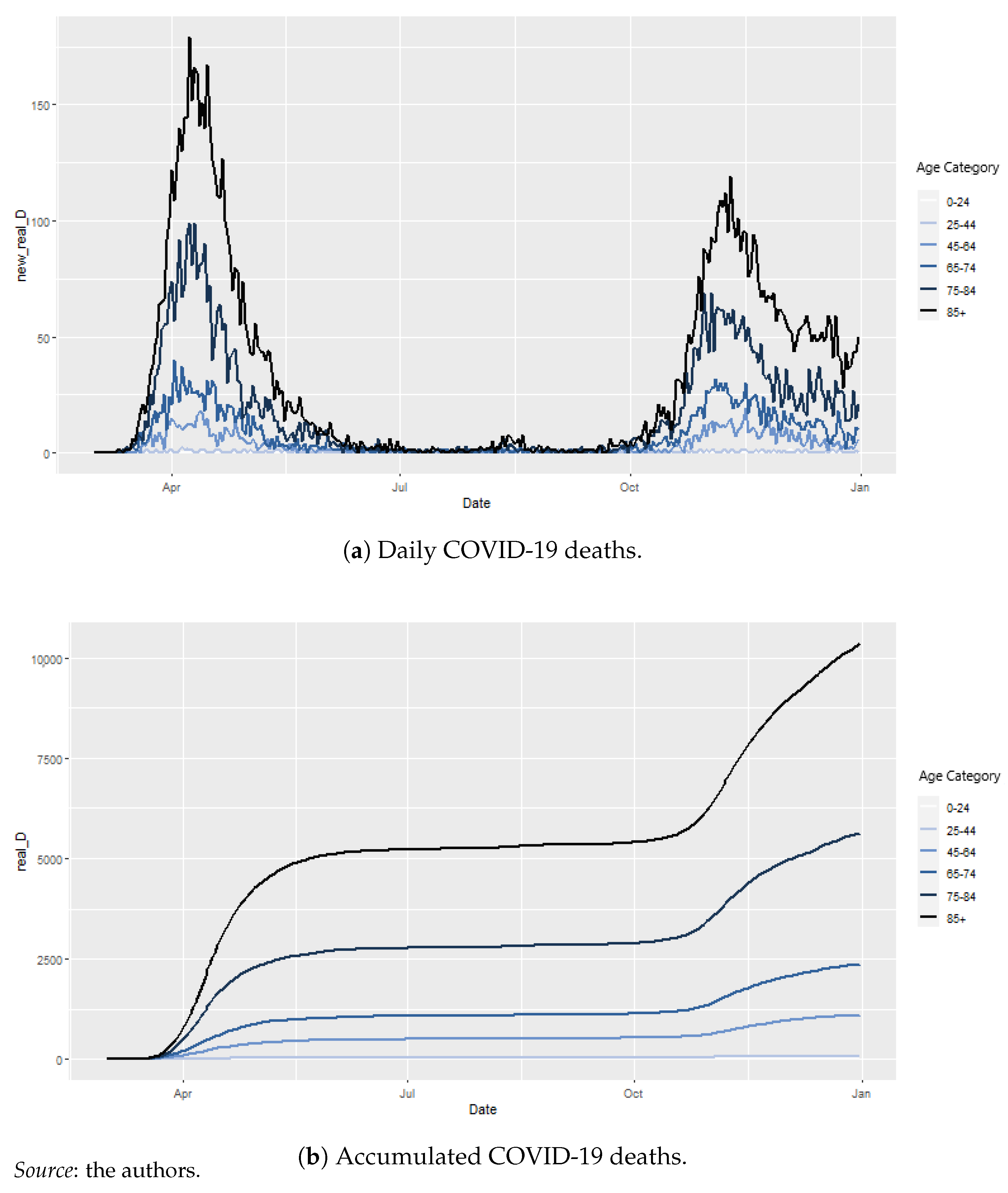
Figure 2a,b depict the daily and cumulated COVID-19 deaths, respectively. The two main waves appear clearly in the figures. Furthermore, the particular virulence to old age is clear, as most deaths belong to the 75–84 and 85+ age categories. We used the Human Mortality Database (2021)6 database for global mortality. Our study is reduced to the year 2020.
4.2. Epidemiological Model
4.2.1. Parameters
In order to simulate the model, we need to identify the following parameters:
- the initial conditions: N, , ;
- the social contract matrix: C;
- COVID-19-related parameters: , , , and .
Some parameters are based on assumptions, as they represent demographics or the biological and medical nature of the problem and are given by scientific articles. Others were found using optimization. We used the root mean square error (RMSE) to assess the quality of our model. In particular, we compared raw data with estimated daily deaths:
for
- corresponds to 1 March 2020, and T corresponds to either for 31 October 2020 for the preliminary model7 and for 31 December 2020 for the model with delay and final model;
- is the daily number of deaths predicted by the model for day, t, and age group, i, given by
- is the real number of daily deaths for time, t, and age group, i.
We assessed our models graphically by comparing realized deaths, cumulated deaths, and death surges with the modeled versions. We studied three models:
- Model with delay: This model relies on the values that coincide between the two waves but uses , which was estimated for our database;
- Final model: This model relies on the values that differ between the two waves and uses the estimated , which was fine-tuned to the differences observed between the two waves.
The model with delay and final model rely on data for the whole pandemic period from 01-03-2020 to 31-12-2020. In what follows, we present the parameters that were used in our model and specify (where needed) whether these parameters are relevant for all the models or not.
- : the Belgian population, as of 1 January 2020 per age category, is given in Table 1:
- : Number of deaths reported until 2 March 2020 (Sciensano 2021);
- : The social contact matrix, which is based on the Socrates tool from Willem et al. (2020);
- : is determined using , according to the following equation:
4.2.2. Preliminary Model
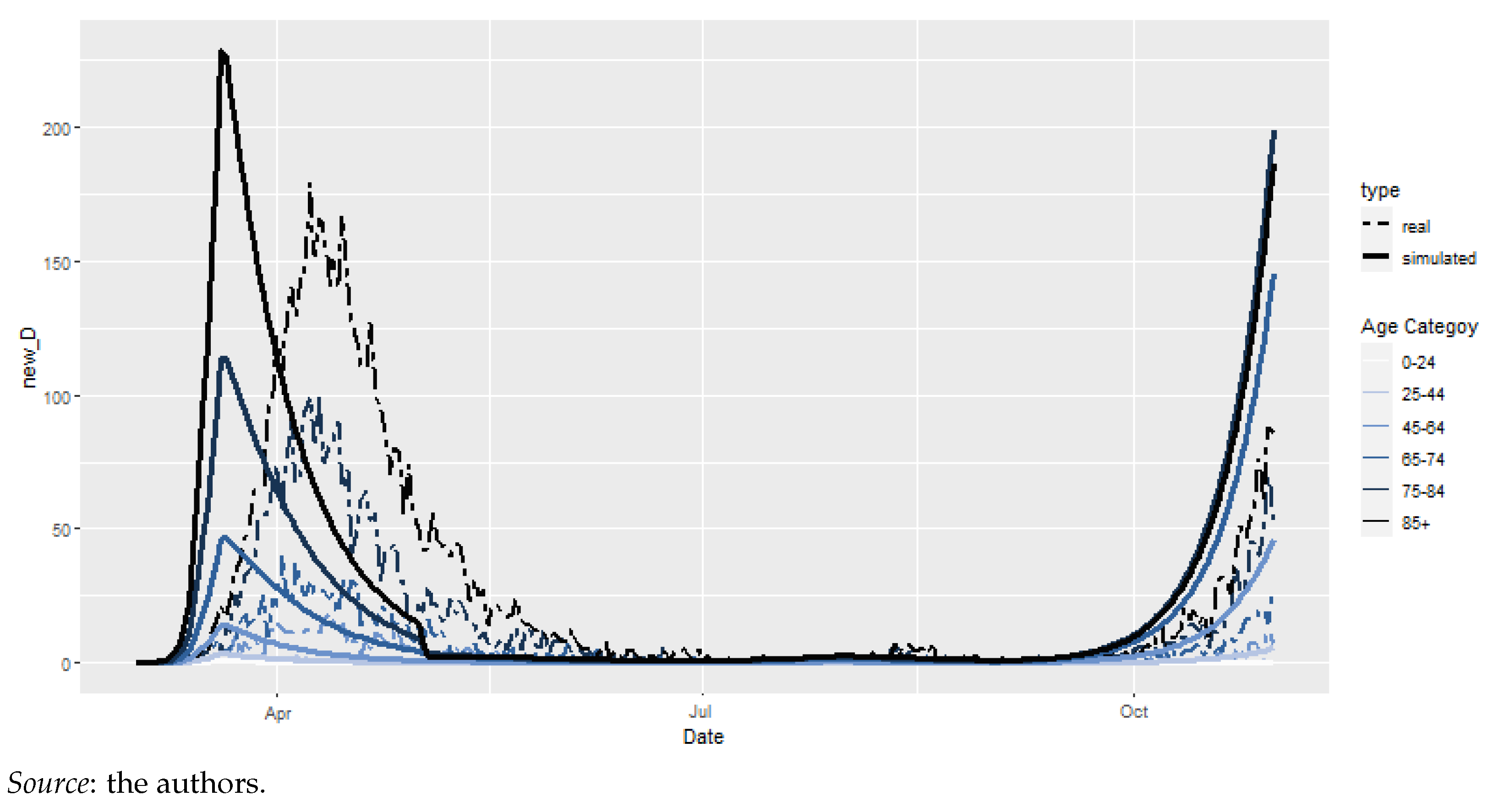
As discussed in Section 3.1, we solved the ODE system (1) by using a multistep methodology. We used the R package deSolve for this. The model is used for the period between 1 March 2020 and 31 October 2020 for the reasons explained earlier in Section 4.2.1. By using the values from Table 3 from Franco (2021) for an adjusted initial number of infected individuals = 6 in the 25–44 age category, we obtained an RMSE of 402.3329.
Figure 3 depicts the difference between the simulated and actual daily deaths. Two obvious trends appear: death is over-estimated in this model, and there is a clear delay in the pandemic peaks. It becomes obvious that relying on pre-specified values does not provide satisfactory results; hence, we need to calculate it ourselves.
4.2.3. Parameter Calculation
The need to have a more granular study of appeared in the previous study. We calculated the value of for shorter time intervals corresponding to changes in policy to fight the pandemic. For instance, we separated the period of 19/03–03/05 and 04/05–07/06 in 19/03–03/04 for the full lockdown and 04/04–07/06 for Phase 1 and 2 of the post-lockdown period, better reflecting the restrictions. Table 6 provides a summary of the periods considered.
First, we calculated the parameter according to the period division proposed in Table 6. Given the time-intensive procedure, parallel computing was carried out in R. The models obtained were compared with regard to their RMSE. We separated the first and second waves in the calculation of . Table 7 highlights the computational time for an array of parameter sets and the number of cores used in parallel computing.
The best model, according to the RMSE calculation, yields the model depicted in Figure 4. There is a clear delay between the peaks and valleys of the simulated model vs. reality. Indeed, our simulated peak is for 20/03/2020, whereas the real peak is observed for 08/04/2020, indicating a 18-day delay. We denote this model as model with delay.
Multiple a priori reasons could be raised in order to understand this delay. The first explanation lies in the recovery rate, . This empirically varies between the two waves, whereas our preliminary model considered the same for the whole period of 2020. Hence, we used a new set of parameters for recovery, assuming a longer recovery period during the first wave compared to the second wave. The new parameters are given in Table 8. A second explanation lies in the calculation of . This parameter changes much faster at the beginning of the pandemic than it does during the second wave. Utilizing the same time step for the calculation of may seem misleading. Instead, a weekly step was adopted from 01-03 to 09-04.
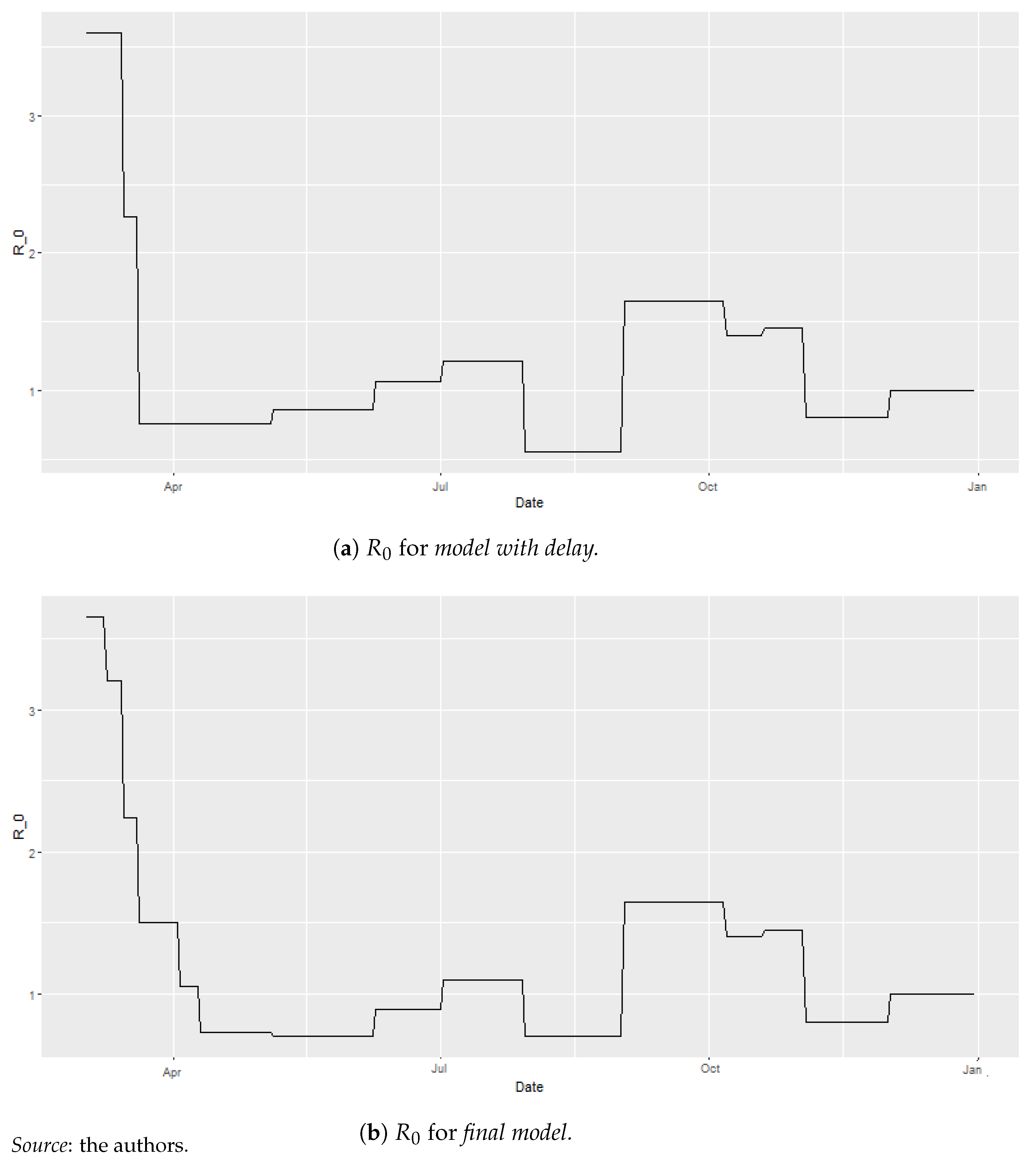
In Figure 5a,b, we observe the parameters for model with delay and final model, respectively. We clearly see the need for a finer grid in order to replicate the rapid evolution of at the beginning of the pandemic10. The former grid yielded strong jumps.
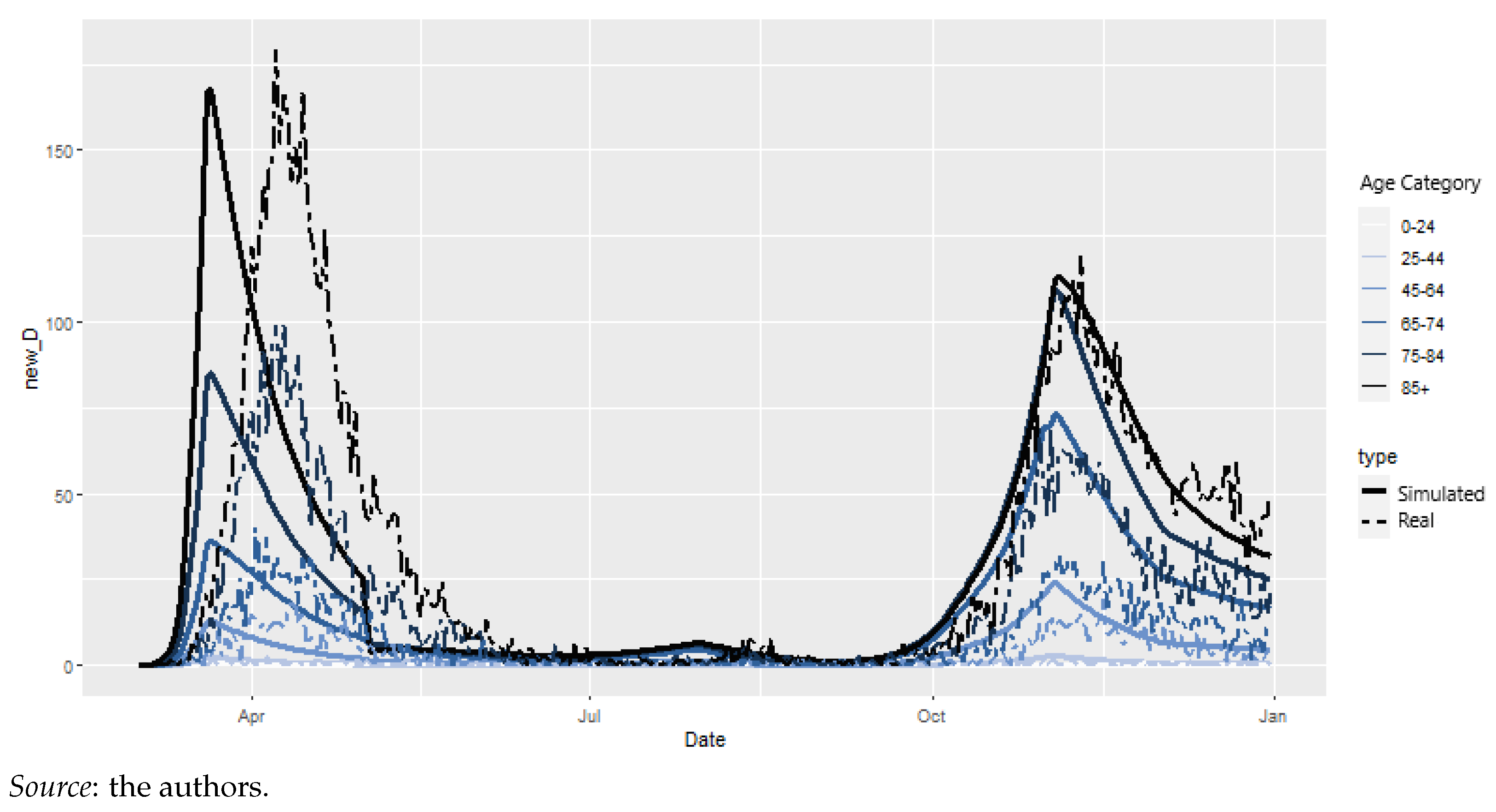
Of course, we could consider working on a finer grid for the whole duration of the study. However, computational time would be greatly affected. Using a weekly time step for the whole study would yield a number of parameter sets equal to 2,377,728, which would take 10 days and 17 h to fit. Furthermore, In Figure 6, we observe that the enhanced model fits the raw data reasonably well. Indeed, incorporating the new calculation and recovery rates yields a first wave peak at 08/04/2020, coinciding with the raw data. Hence, we reduced the time step to a weekly basis for the beginning of the first wave but kept the longer time step for the remainder of the analysis. We denote this model as final model.
Finally, we compare the three models, preliminary model, model with delay, and final model, with regard to their RMSE (Table 9). We distinguish two time periods: Period 1, which covers up until 31/10/2020, and Period 2, which covers up until 31/12/2020. Of course, preliminary model does not have a value for Period 2 because the values of Franco (2021) were only available until 31/10/2020, thus limiting our preliminary study up to that period. It is clear that our final model outperforms the others in terms of RMSE.
4.2.4. Epidemiological Model: Results
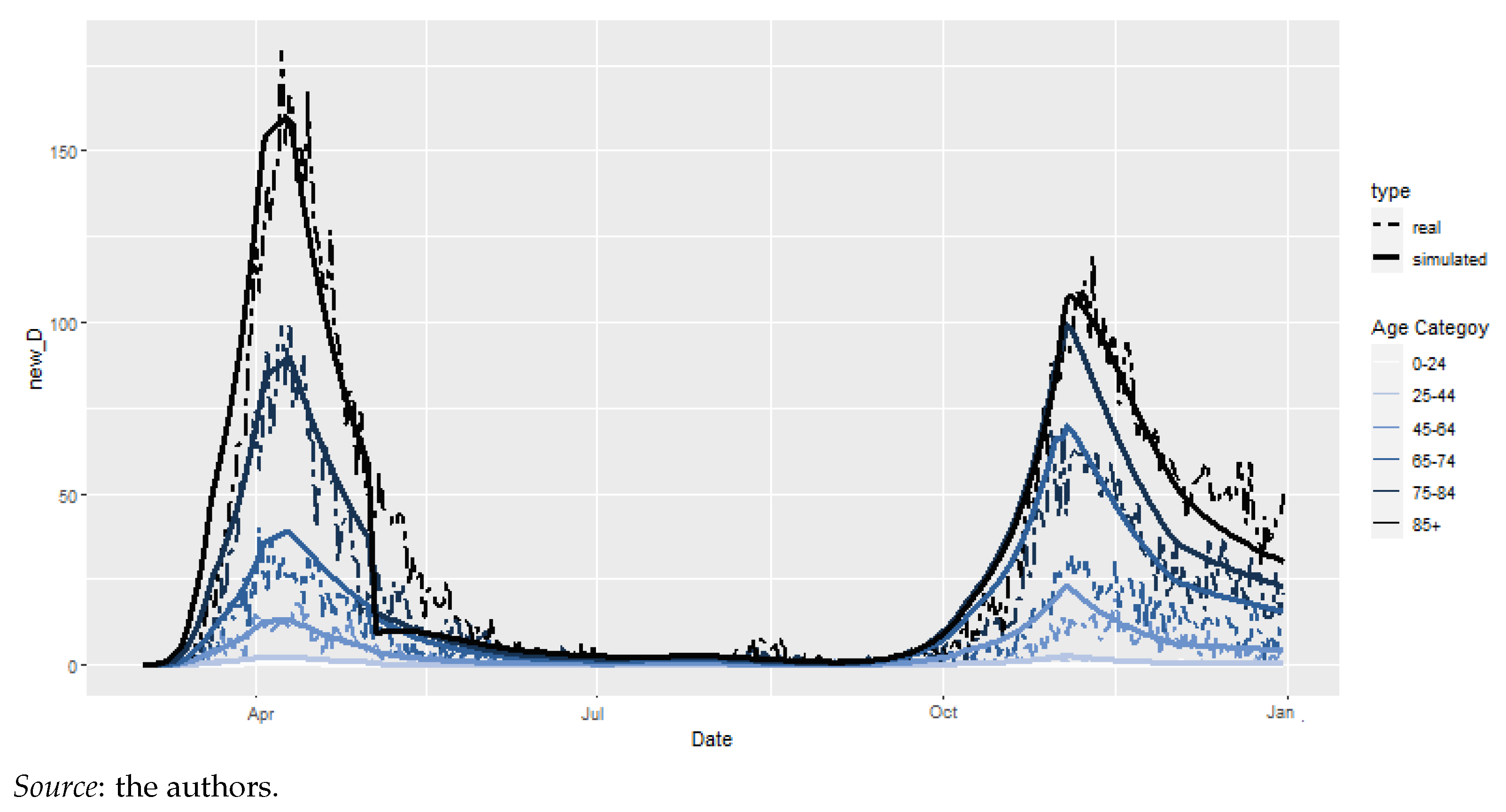
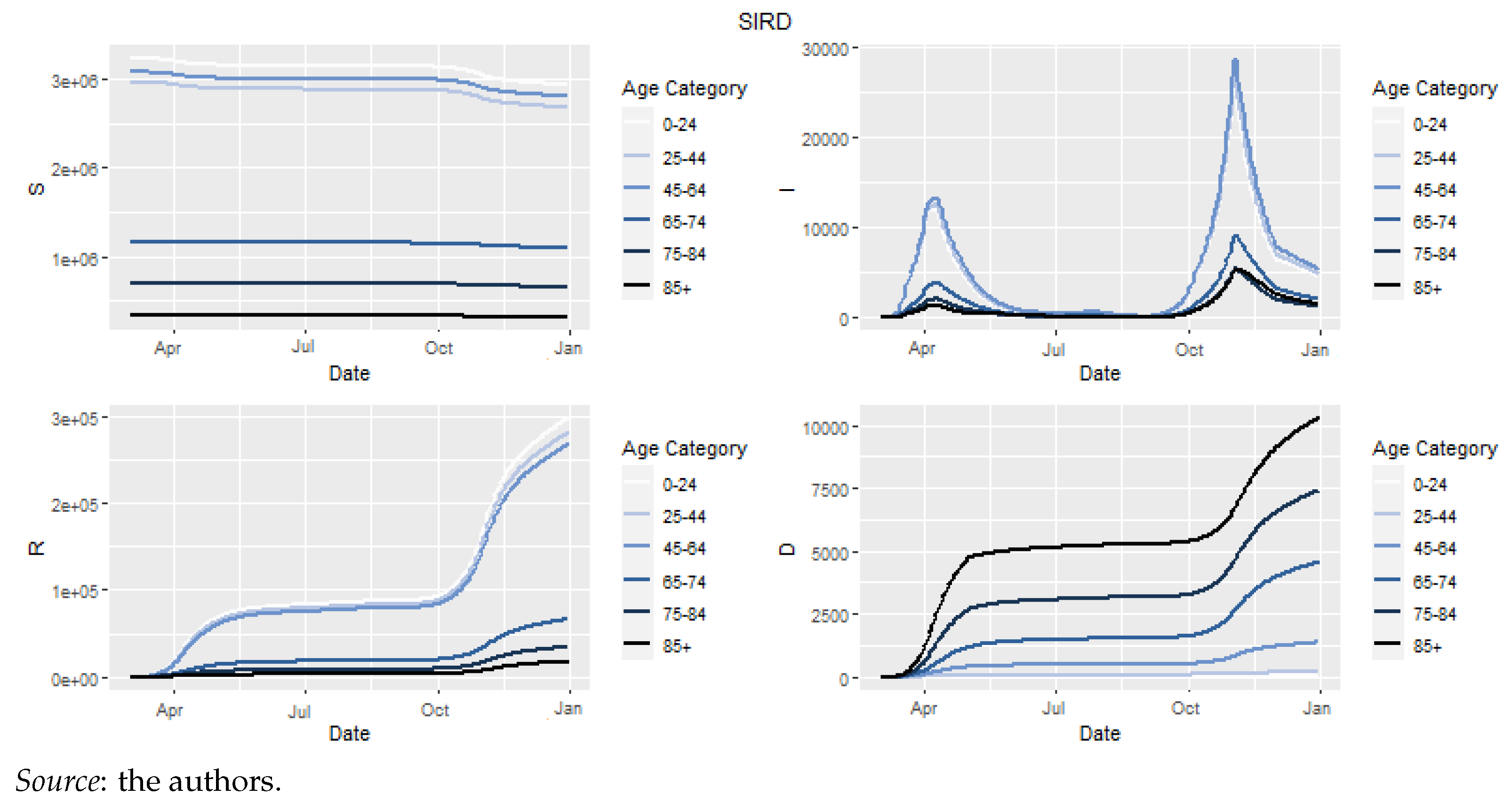
Figure 7 depicts the evolution of Susceptible, Infectious, Recovered et Dead as the solutions of final model.
The graph for infectious clearly shows the two waves of the epidemic. Despite the greatest number of sick individuals existing during the second wave, the deaths were more numerous during the first wave. Our solution also allows us to calculate the empirical mortality rate. These empirical mortality rates, when merged with global mortality, allowed us to assess the effect of excess mortality within a life insurance product context.
The empirical mortality rates were calculated using the number of deaths per age category, given by the model together with the estimated , as per Equation (6). With the exposure data not available for 2020, we approximated them by using . The obtained results can be seen in Table 10.
When compared to the actual data, Table 10 indicates that COVID-19-related death is overestimated for the 25–44, 65–74, and 75–84 groups, whereas it provides very reliable estimates for the 45–64 and 85+ groups. This was already apparent from Figure 6, as the latter age categories are those for which the curves and real date correspond the best. Note that deaths over 85+ years amount to over 50% of the total deaths; hence, this reveals the importance of having accurate estimates for this later age group (O’Driscoll et al. 2021).
4.3. Cairns-Blake-Dowd Model
We need base mortality in order to be able to assess excess mortality. Here, we focus on the fit of the Cairns et al. (2006) model for Belgium by using the Human Mortality Database (2021). We calibrated the model from 1968 to 2018, which includes the last year available under the Human Mortality Database (2021), using the StMoMo package in R. We refer to Appendix A for details regarding period selection, estimation, residual analysis, and forecast.
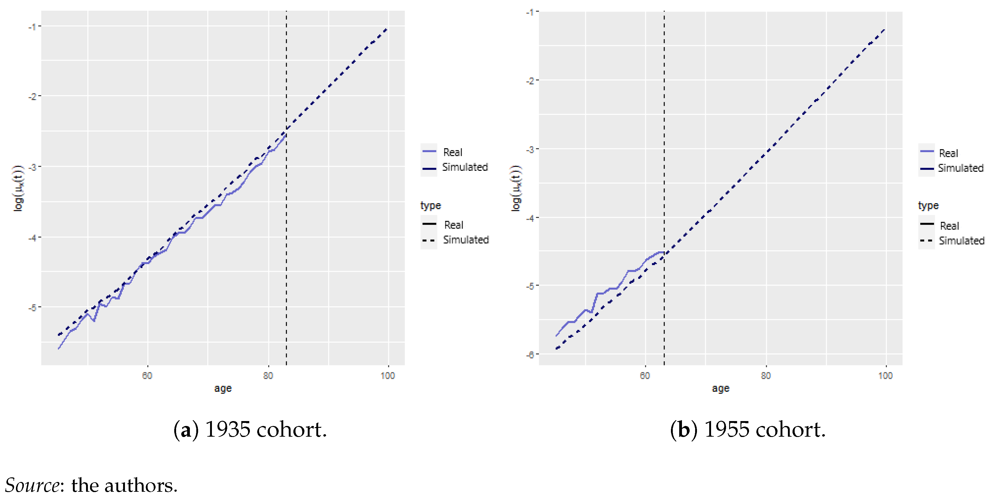
We analyzed the effect of COVID-19 mortality on life insurance products. This was carried out for various cohorts to assess the relative impact of the pandemic on recent contracts vs. contracts underwritten in 2000. In particular, we are interested in studying the male cohort born in 1935 and the second male cohort born in 1955.11 Figure 8a,b show the fitted model (discontinued line) vs. empirical mortality rates (blue continuous line), as given by the maximum likelihood estimator for the two cohorts of interest. It is clear that the mortality rate for the 1935 cohort is greater than that of the 1955 cohort, which clearly follows from the fact that the former was born during World War II. The vertical dotted line represents the age from which no empirical data are available.12
4.4. Model Reconciliation
By agggregating the mortality rates obtained in Section 4.2.4 and Section 4.3, we obtained the COVID and no-COVID scenarios for . Of course, as long as , we will see some excess mortality since . The treatment of COVID-19 as a parallel shift aligns with the empirical evidence found by Spiegelhalter (2020). In the remainder of the manuscript, we assess the extent of this excess of mortality and whether it greatly impacts life expectancy and product valuation.
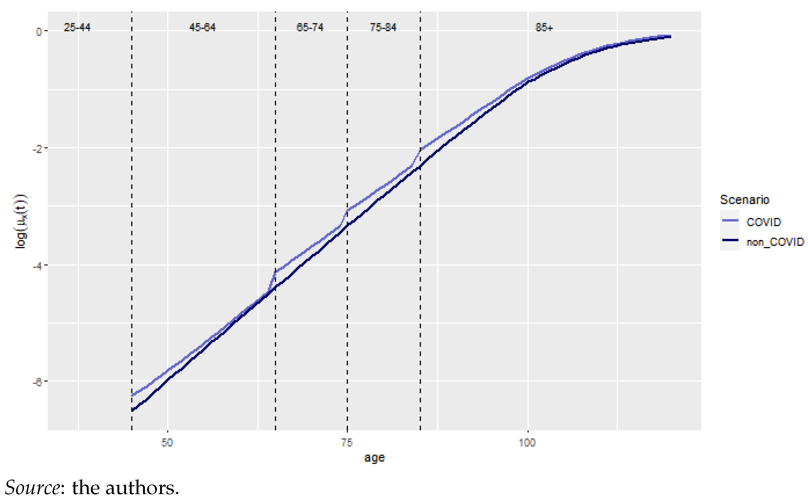
The log mortality rates for the year 2020 for the two scenarios are presented in Figure 9. The vertical discontinuous lines represent the age categories, the blue and black lines represent the COVID and no-COVID scenarios, respectively. We observe a jump upon each age category change. These are explained by considering the differences between natural mortality and excess of mortality for the first part of the age interval. Indeed, let us focus on the 75-84 group to clarify this. Relatively speaking, the excess of mortality is much more important for a person aged 75 years with respect to someone aged 84 years since is constant for a particular age category.13
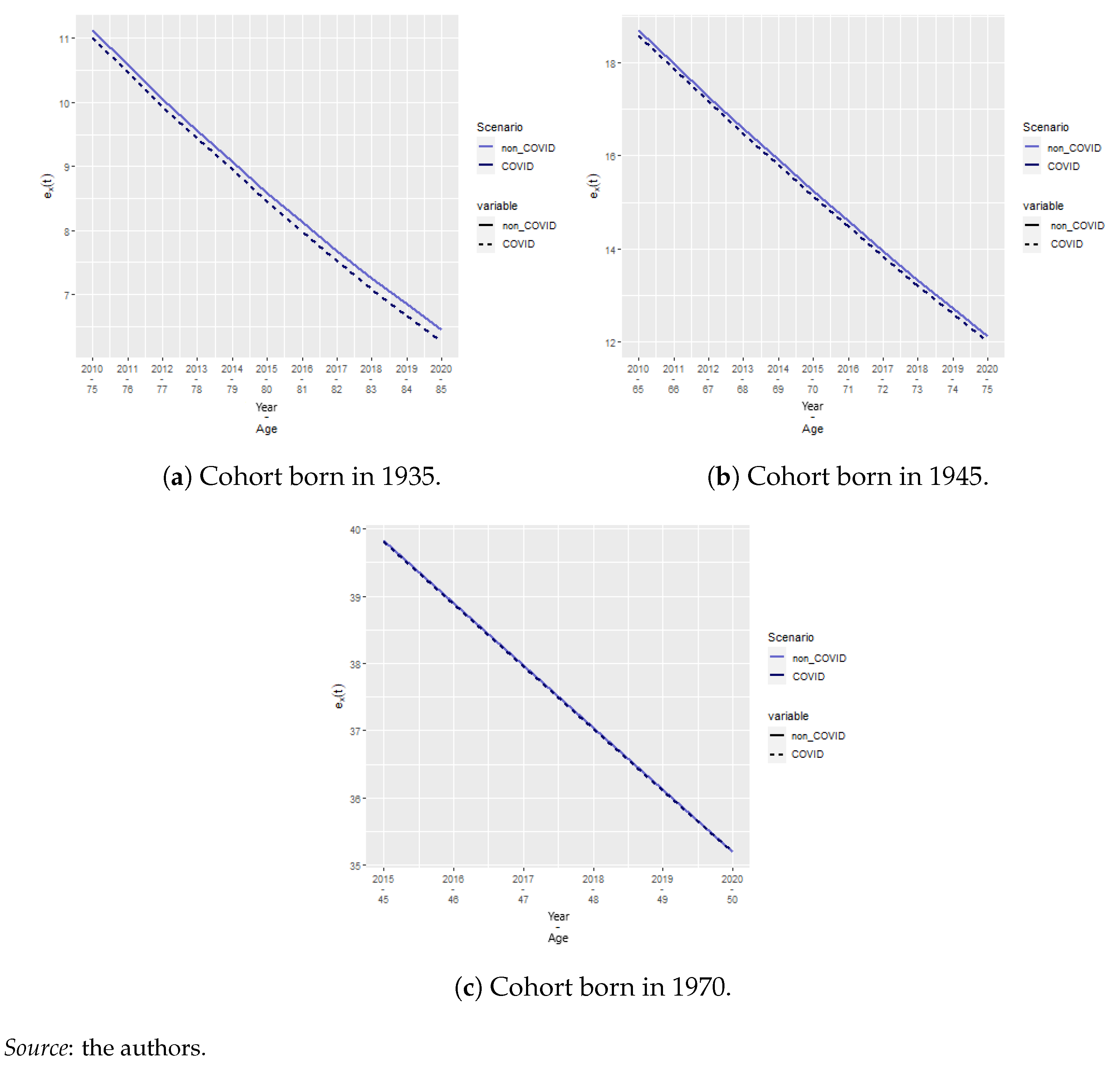
We also calculated the cohort life expectancies using Equation (15) for the cohorts born in 1935, 1945, and 1970 for the COVID and no-COVID scenarios (Figure 10a–c) aged 75, 85, and 50 years in 2020, respectively. We observe that the relatively large differences in the log mortality rate do not translate to extreme differences in cohort life expectancy, especially for old ages. We observe that the older the cohort, the greater the effect of COVID-19. However, this effect lasts, at most, for 3 months. Hence, we deduce that the effect of COVID-19 on lifetime annuity pricing might also be reduced.
4.5. Actuarial Application
We studied a whole life insurance policy, paying EUR 20,000 (=C) in capital at the end of the year of death to the insured’s beneficiary. The second product is a lifetime annuity (immediate), paying EUR 2000 (=P) per month while the insured is alive. We priced this at a technical rate of . These products have an inverse relationship with mortality. Indeed, an adverse mortality shock will increase the price of a whole life insurance, whereas it will decrease the price of a lifetime annuity as death becomes more likely.
We consider two cohorts as per the underwriting year. We studied cohorts born in 1970 and 1955 for the contracts underwritten in 2019, a year before the pandemic. These people were 49 and 64 years old at underwriting and 65 and 50 years old during the pandemic. We considered cohorts born in 1945 and 1935 for contracts underwritten in 2000. These people were 55 and 65 years old at underwriting and 85 and 75 years old during the COVID-19 year of 2020. Furthermore, we considered the effect of COVID-19 excess mortality during the year 2020 by studying with and without scenarios. The NPV, its variance (as presented in Section 3.4), and the relative difference between COVID and no-COVID scenarios given by Equation (29) were analyzed:
We also studied the difference between the no-COVID case and the catastrophic COVID scenario, whereby
Table 11 shows the NPV and standard deviation for the base COVID case, corresponding to the estimated mortality presented in the previous sections for the whole life insurance (left block) and lifetime annuity (right block). For the whole insurance case, we observe that the NPV increases in the presence of COVID-19, as is expected. Indeed, higher mortality increases the likelihood of paying the capital, which increases according to the NPV. On the contrary, the NPV of the annuity decreases in the presence of COVID-19. However, as in the case of whole life insurance, the variation is negligible.
The standard deviation, on the other hand, has a more interesting trend. Indeed, for both insurance products, we observe that the variance increases for the contracts underwritten just before the pandemic to younger individuals, whereas it decreases for old contracts. Table 12 presents the effect of a catastrophic COVID scenario, where the mortality rate is multiplied by 10. We see that the relative change in NPV corresponds to roughly 10 times as well. Similarly, the decreases or increases in variance are almost 10-fold. Our results align with Carannante et al. (2022) and Schnürch et al. (2022), whereby the annuity premiums decrease and the death-contingent insurance products increase, as is expected.
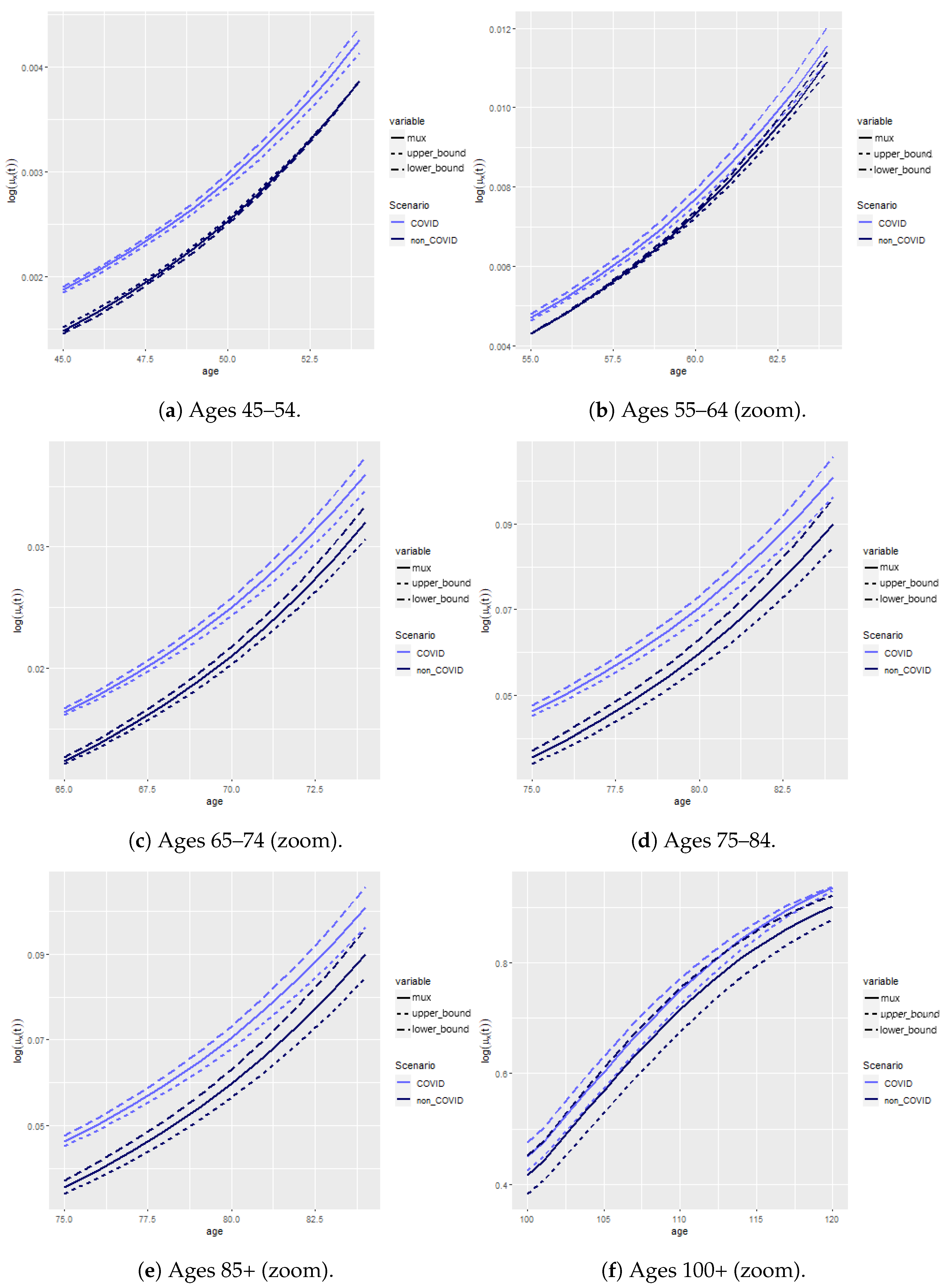
We found that variance changed depending on whether the contract was underwritten soon or long before the start of the pandemic. This aligns with the results found in Schnürch et al. (2022)14. Indeed, we see a higher variability for contracts underwritten close to the pandemic; in our case, 1 year prior the pandemic outburst. The worst possible outcome is to have a variance increase, which is the case for contracts underwritten in 2019 to individuals aged 49 and 64 years old. On the contrary, old contracts see their variance decrease. This is linked to the behavior of the confidence intervals (CI) of the mortality rates, which we depict in Figure 11. This graph shows the CI for all age categories, with an adjusted scale to see the differences between the two scenarios.
Obviously, mortality is greater in the presence of COVID-19 for all ages. However, the variability varies. Indeed, we observe wider bounds in the presence of COVID-19 prior to retirement (Figure 11a,b), with slightly greater levels of uncertainty for ages 65–74 (Figure 11c) and narrower bounds beyond the age of 75 (Figure 11d–f). We hypothesize that this is due to deaths being more unlikely in normal circumstances before retirement, so every additional death due to COVID yields a more uncertain outcome and affects the CI and variability of the insurance products accordingly. After retirement, it has the opposite effect, as natural deaths are more common, and COVID-19 renders this even more likely, narrowing down the CIs of the mortality rates and contracts for those insured at these ages accordingly.
Hence, the CI widens for younger ages, whereas it narrows for older ages in the presence of COVID-19. The narrowing (widening) of the CIs translates to a reduction (increase) in the standard deviation, respectively. The consequences of such a pandemic scenario show clear risks: for products that pay in the event of death, we have a risk of underpricing, and overall, we can observe a volatility increase that would put our reserves and capital levels at risk.
5. Conclusions
This paper provides an actuarial analysis based on excess mortality in the context of COVID-19. We developed an epidemiological model to estimate COVID-19-related mortality in Belgium in 2020 and reconciled it with an aggregate mortality model. In this way, we contribute to recent actuarial work on the epidemiological models of Feng and Garrido (2011), Chen et al. (2021), and Hall et al. (2020). We extend the work of Feng and Garrido (2011) by considering a SIRD component with a death compartment, and we extend the work of both Feng and Garrido (2011) and Chen et al. (2021) by adding age categories inspired by recent epidemiological work of Balabdaoui and Mohr (2020) for Switzerland and Franco (2021) for Belgium.
We present a SIRD epidemiological model that relies on data-specific . This results in a model that very accurately reflects the number of deaths for different age categories and shows accurate timing with regard to the peaks and valleys. From an empirical epidemiological perspective, we extend the work of Franco (2021) to the full year of 2020, whereas their study is limited to 31 October 2020 due to data constraints.
We find that considering COVID-19 increases the net present value (NPV) of whole life insurance and decreases the NPV of lifetime immediate annuity as expected. We find that the variability of the contract increases for recently underwritten contracts, whereas the variability decreases for old contracts, and this is true for both insurance products. We hypothesize this is due to COVID-19 rendering death at older ages more certain, decreasing the variability of such products. In all cases, the level of standard deviation change remains limited, akin to the results found in Carannante et al. (2022).
Our work is comprehensive but has various aspects that can be improved. The study is limited to 1 year of COVID-19-related mortality data. Adding more years, combined with the various age categories, would raise the need to create a transition mechanism between the age categories; this could be added within the ODE system. Furthermore, our model reflects the main compartments of interest in the context of an insurance application, be it recovery or death, as payments are contingent on either survival or death. It does not reflect other aspects of the pandemic, such as quarantine, incubation, or hospitalization. Finally, due to data limitations, we have abstracted our results by considering the effect of COVID-19 on the global health landscape. Indeed, one of the challenges of the pandemic has been managing the sudden inflow of sick people into intensive care units. This obviously has had a (negative) effect on the treatment of other diseases, for which the short- and long-term effects are still unknown.
Author Contributions
Conceptualization, J.A.-G.; Formal analysis, C.D.; Methodology, J.A.-G.; Supervision, J.A.-G.; Visualization, C.D.; Writing—original draft, C.D.; Writing—review and editing, J.A.-G. All authors have read and agreed to the published version of the manuscript.
Funding
This research received no external funding.
Data Availability Statement
All data sources have been duly cited.
Acknowledgments
This project was carried out while Camille Delbrouck was a MSc student at ULB. We thank the Society of Actuaries and attendees of 2023 Living to 100 conference attendees in Orlando, Florida, 16–18 January 2023, and Kowloon, Hong Kong, 16 February 2023. The authors are responsible for any errors.
Conflicts of Interest
Author Camille Delbrouck was employed by the company Aon Benfield. The remaining authors declare that the research was conducted in the absence of any commercial or financial relationships that could be construed as a potential conflict of interest.
Appendix A. Cairns, Blake, and Dowd Estimation and Analysis
Appendix A.1. Estimation
The theoretical methodological procedure is detailed in Section 3.2. We calibrated the model from 1968 to 2018, which includes the last year available under the Human Mortality Database (2021), by using the StMoMo package in R.15 This period is chosen as a linear trend becomes clear from 1968, as shown in Figure A1. We consider the age period 45 to 100 years, excluding the accident hump that would, otherwise, be poorly fitted by this model. Furthermore, we are solely interested in the effect of COVID-19 and its insurance products for adults and old ages since COVID-19 mortality rates are negligible under the age of 44 (Table 10).
Figure A1.
Choice of time period.

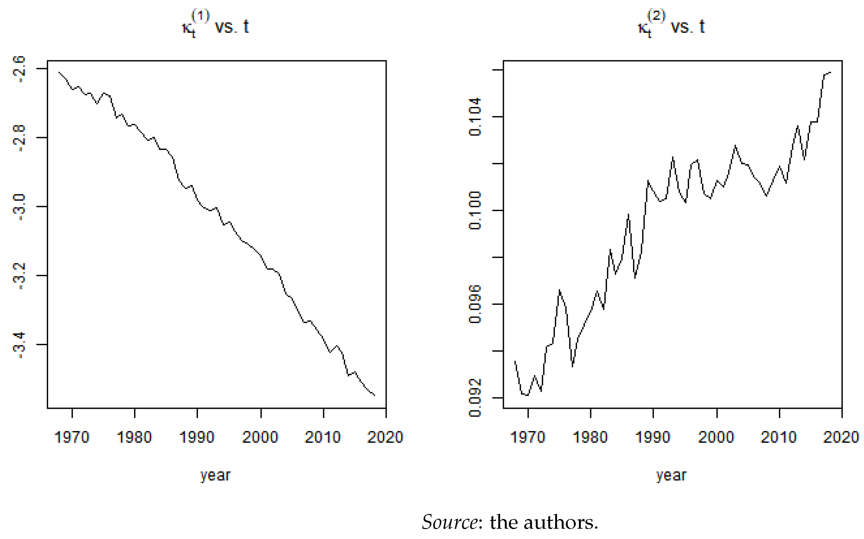
Figure A2 shows the estimated parameters for the age and period interval chosen. The trends observed coincide with expectation, decreases over time, reflecting mortality improvements, whereas increases, indicating that the improvements have been more important under than beyond the mean age considered in our study.
Figure A2.
CBD fit.

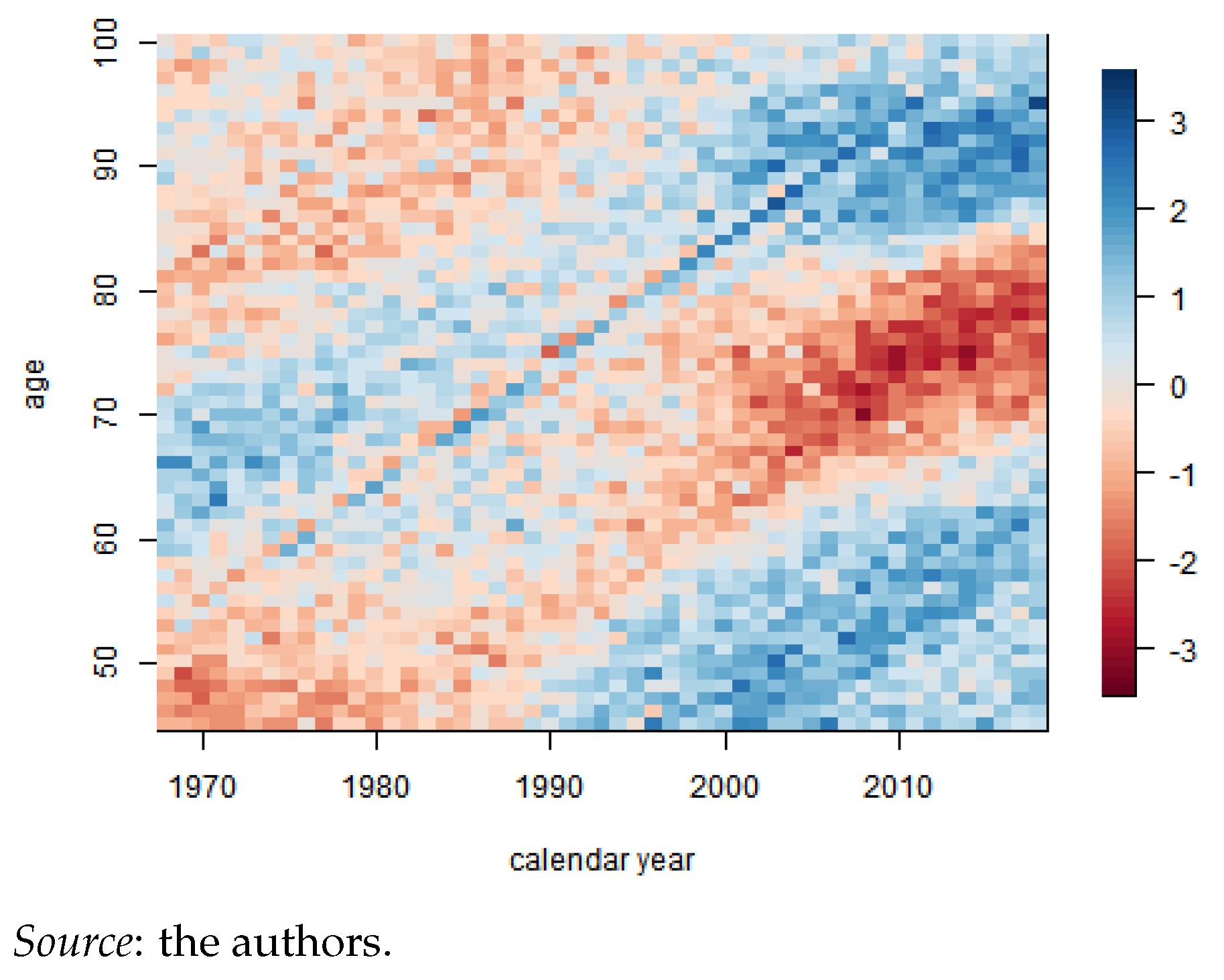
Residuals are calculated as per Equation (11) and are depicted in Figure A3. We observe no clear trends beyond a reduced cohort effect for the individuals born in 1920 after the First World War.
Figure A3.
Residual heatmap.

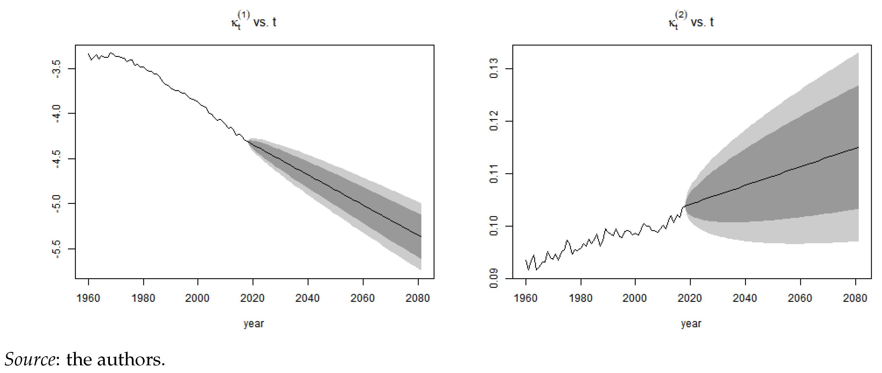
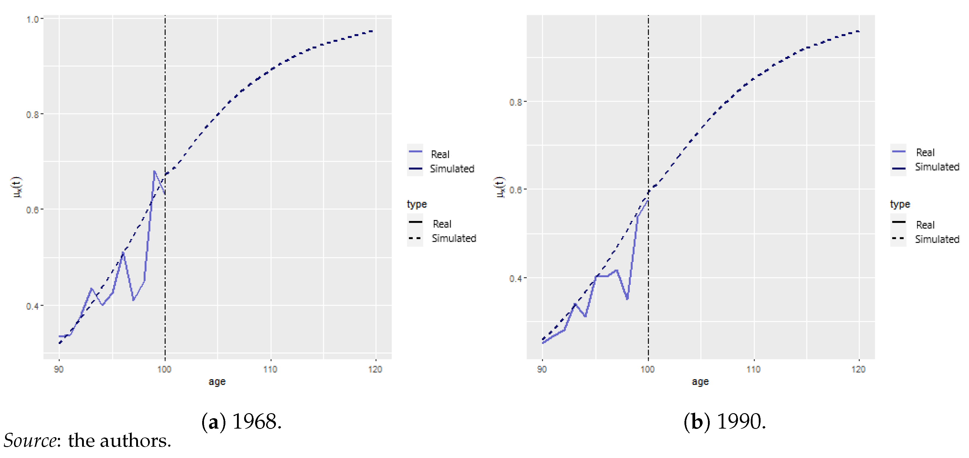
Appendix A.2. Mortality Projection and Extrapolation
We projected , as indicated in Section 3.2, and obtained the trends depicted in Figure A4. With unsatisfactory data beyond the age of 100, we performed the logistic regression, indicated in Equation (14), by using , allowing us to project mortality rates, , until = 120, the ultimate age. The results are given in Figure A5a,b. The vertical dotted line indicates the start of the logistic extrapolation. The discontinued line depicts the modeled rates, whereas the blue lines correspond to the historical information.
Figure A4.
Projection of and .

Figure A5.
Old age logistic regression.

| 1 | The yearly seasonal flu does not fall within the scope of our study, being a recurrent sickness. Our aim is to model a one-off pandemic caused by a new virus as distinguished by the CDC. |
| 2 | The SIS model is commonly used to model the common cold or the flu as infection does not provide long-term immunity. |
| 3 | The recovered state is absorbent. This was a reasonable hypothesis in 2020, the year in which the model was parametrized. COVID infection was assumed to provide long-term immunity. The models that allow for recovery could address this but they are outside the scope of this study due to data limitations. |
| 4 | This is in contrast to one-period methodologies, such as the Euler method, which solely refers to a previous point and its derivative to determine the actual value, or the Runge-Kutta method, which uses a few intermediate points but rejects all previous points to obtain a higher-order value. |
| 5 | This package relies on generalized linear models and uses the package gnm to solve for numerous stochastic mortality models that can be expressed within a GLM framework. The algorithm follows two steps. Firstly, the nonlinear parameters are updated, and then the linear parameters are. Secondly, all parameters are updated jointly until convergence is attained. |
| 6 | The Human Mortality Database was created to provide detailed data about population and mortality to researchers, students, journalists, political analysist and individuals interested in the history of human longevity. |
| 7 | |
| 8 | It is time-dependent because the lockdown and quarantine rules have changed according to the evolution of the pandemic. |
| 9 | Mortality rates for Belgium were studied in various studies (Levin et al. 2020; Molenberghs et al. 2020). The meta-study from Levin et al. (2020) finds the relationship . However, these results are not wave-dependent. |
| 10 | This corresponds to the following intervals in the final model: 1/3/2020, 8/3/2020, 14/03/2020, 19/03/2020, 26/03/2020, 2/4/2020, 9/4/2020, 4/5/2020, 8/6/2020, 1/7/2020, 29/07/2020, 1/9/2020, 6/10/2020, 19/10/2020, 2/11/2020, 1/12/2020, 24/12/2020, and 31/12/2020. |
| 11 | Details about the characteristics of the contract are given in Section 4.5. |
| 12 | Obviously, the 1935 and 1955 cohorts were 83 and 63 years old in 2018, whcih is the last observed year according to Human Mortality Database (2021), making it impossible to compare with empirical data beyond these ages. |
| 13 | In reality COVID related mortality will most likely vary within the age category. However, we are unable to extract this trend due to data limitations. |
| 14 | Carannante et al. (2022) only provide point estimates of their insurance product valuation. |
| 15 | Missing values, as wel as NA, are associated zero weight and are hence not included in the fit. |
References
- Abou-Ismail, Anas. 2020. Compartmental models of the COVID-19 pandemic for physicians and physician-scientists. SN Comprehensive Clinical Medicine 2: 852–58. [Google Scholar] [CrossRef] [PubMed]
- Arnold, Séverine, and Michael Sherris. 2013. Forecasting mortality trends allowing for cause-of-death mortality dependence. North American Actuarial Journal 17: 273–82. [Google Scholar] [CrossRef]
- Arnold, Séverine, and Michael Sherris. 2015. Causes-of-death mortality: What do we know on their dependence? North American Actuarial Journal 19: 116–28. [Google Scholar] [CrossRef]
- Balabdaoui, Fadoua, and Dirk Mohr. 2020. Age-stratified discrete compartment model of the COVID-19 epidemic with application to switzerland. Scientific Reports 10: 1–12. [Google Scholar] [CrossRef]
- Boumezoued, Alexandre, Héloïse Labit Hardy, Nicole El Karoui, and Séverine Arnold. 2018. Cause-of-death mortality: What can be learned from population dynamics? Insurance: Mathematics and Economics 78: 301–15. [Google Scholar] [CrossRef]
- Cairns, Andrew J. G., David Blake, and Kevin Dowd. 2006. A two-factor model for stochastic mortality with parameter uncertainty: Theory and calibration. Journal of Risk and Insurance 73: 687–718. [Google Scholar] [CrossRef]
- Calafiore, Giuseppe C., Carlo Novara, and Corrado Possieri. 2020. A modified sir model for the COVID-19 contagion in italy. Paper presented at the 2020 59th IEEE Conference on Decision and Control (CDC), Jeju, Republic of Korea, December 14–18; pp. 3889–94. [Google Scholar]
- Carannante, Maria, Valeria D’Amato, and Steven Haberman. 2022. COVID-19 accelerated mortality shocks and the impact on life insurance: The italian situation. Annals of Actuarial Science 16: 478–97. [Google Scholar] [CrossRef]
- CDC. 2021. 1918 Pandemic (h1n1 Virus). Available online: https://www.cdc.gov/flu/pandemic-resources/1918-pandemic-h1n1.html (accessed on 24 May 2021).
- Chen, Xiaowei, Wing Fung Chong, Runhuan Feng, and Linfeng Zhang. 2021. Pandemic risk management: Resources contingency planning and allocation. Insurance: Mathematics and Economics 101: 359–83. [Google Scholar] [CrossRef] [PubMed]
- Feng, Runhuan, and Jose Garrido. 2011. Actuarial applications of epidemiological models. North American Actuarial Journal 15: 112–36. [Google Scholar] [CrossRef]
- Feng, Runhuan, José Garrido, Longhao Jin, Sooie-Hoe Loke, and Linfeng Zhang. 2022. Epidemic compartmental models and their insurance applications. In Pandemics: Insurance and Social Protection. Edited by María del Carmen Boado-Penas and Julia Eisenberg. Cham: Springer International Publishing, pp. 13–40. [Google Scholar]
- Fernández-Villaverde, Jesús, and Charles I. Jones. 2022. Estimating and simulating a sird model of COVID-19 for many countries, states, and cities. Journal of Economic Dynamics and Control 140: 104318. [Google Scholar] [CrossRef]
- Franco, Nicolas. 2021. COVID-19 belgium: Extended seir-qd model with nursing homes and long-term scenarios-based forecasts. Epidemics 37: 100490. [Google Scholar] [CrossRef] [PubMed]
- Hall, R. Dale, Cynthia S. MacDonald, Peter J. Miller, Achilles N. Natsis, Lisa A. Schilling, Steven C. Siegel, and J. Patrick Wiese. 2020. Society of Actuaries Research Brief: Impact of COVID-19. Technical Report. Itasca: Society of Actuaries. [Google Scholar]
- Hethcote, Herbert W. 2000. The mathematics of infectious diseases. SIAM Review 42: 599–653. [Google Scholar] [CrossRef]
- Hindmarsh, Alan C. 1983. Odepack, a systematized collection of ode solvers. Scientific Computing 1: 55–64. [Google Scholar]
- Huang, Yubei, Lei Yang, Hongji Dai, Fei Tian, and Kexin Chen. 2020. Epidemic situation and forecasting of COVID-19 in and outside china. Bull World Health Organ 10. [Google Scholar] [CrossRef]
- Human Mortality Database. 2021. Life Tables Belgium 1968–2018—Total (Both Sexes). Available online: https://www.mortality.org/ (accessed on 24 May 2021).
- Institute and Faculty of Actuaries. 2015. Longevity Bulletin 6: The Pandemic Edition. Technical Report. Itasca: Institute and Faculty of Actuaries. [Google Scholar]
- Kermack, William Ogilvy, and Anderson G. McKendrick. 1927. A contribution to the mathematical theory of epidemics. Proceedings of the Royal Society of London. Series A, Containing Papers of a Mathematical and Physical Character 115: 700–21. [Google Scholar]
- Kermack, William Ogilvy, and Anderson G. McKendrick. 1932. Contributions to the mathematical theory of epidemics. ii.—The problem of endemicity. Proceedings of the Royal Society of London. Series A, Containing Papers of a Mathematical and Physical Character 138: 55–83. [Google Scholar]
- Levin, Andrew T., William P. Hanage, Nana Owusu-Boaitey, Kensington B. Cochran, Seamus P. Walsh, and Gideon Meyerowitz-Katz. 2020. Assessing the age specificity of infection fatality rates for COVID-19: Systematic review, meta-analysis, and public policy implications. European Journal of Epidemiology 35: 1123–38. [Google Scholar] [CrossRef]
- Li, Han, Hong Li, Yang Lu, and Anastasios Panagiotelis. 2019. A forecast reconciliation approach to cause-of-death mortality modeling. Insurance: Mathematics and Economics 86: 122–33. [Google Scholar] [CrossRef]
- Li, Hong, and Yang Lu. 2019. Modeling cause-of-death mortality using hierarchical archimedean copula. Scandinavian Actuarial Journal 2019: 247–72. [Google Scholar] [CrossRef]
- Lyu, Pintao, Anja De Waegenaere, and Bertrand Melenberg. 2021. A multi-population approach to forecasting all-cause mortality using cause-of-death mortality data. North American Actuarial Journal 25: S421–S456. [Google Scholar] [CrossRef]
- Molenberghs, Geert, Christel Faes, Johan Verbeeck, Patrick Deboosere, Steven Abrams, Lander Willem, Jan Aerts, Heidi Theeten, Brecht Devleesschauwer, Natalia Bustos Sierra, and et al. 2020. Belgian COVID-19 mortality, excess deaths, number of deaths per million, and infection fatality rates (9 March–28 June 2020). Euro Surveill. 27: 2002060. [Google Scholar]
- O’Driscoll, Megan, Gabriel Ribeiro Dos Santos, Lin Wang, Derek AT Cummings, Andrew S Azman, Juliette Paireau, Arnaud Fontanet, Simon Cauchemez, and Henrik Salje. 2021. Age-specific mortality and immunity patterns of SARS-CoV-2. Nature 590: 140–45. [Google Scholar] [CrossRef]
- Rogers, Andrei, and Kathy Gard. 1991. Applications of the heligman/pollard model mortality schedule. Population Bulletin of the United Nations 30: 79–105. [Google Scholar]
- Saunders-Hastings, Patrick R., and Daniel Krewski. 2016. Reviewing the history of pandemic influenza: Understanding patterns of emergence and transmission. Pathogens 5: 66. [Google Scholar] [CrossRef] [PubMed]
- Schnürch, Simon, Torsten Kleinow, Ralf Korn, and Andreas Wagner. 2022. The impact of mortality shocks on modelling and insurance valuation as exemplified by COVID-19. Annals of Actuarial Science 16: 498–526. [Google Scholar] [CrossRef]
- Sciensano. 2021. COVID-19 Database. Available online: https://epistat.wiv-isp.be/covid/ (accessed on 24 May 2021).
- Spiegelhalter, David. 2020. Use of “normal” risk to improve understanding of dangers of COVID-19. BMJ 370: m3259. [Google Scholar] [CrossRef]
- Statbel. 2021. Population Structure. Available online: https://statbel.fgov.be/fr/themes/population/structure-de-la-population (accessed on 24 May 2021).
- Tabeau, Ewa, Peter Ekamper, Corina Huisman, and Alinda Bosch. 1999. Improving overall mortality forecasts by analysing cause-of-death, period and cohort effects in trends. European Journal of Population/Revue Européenne de Démographie 15: 153–83. [Google Scholar] [CrossRef]
- Tang, Lu, Yiwang Zhou, Lili Wang, Soumik Purkayastha, Leyao Zhang, Jie He, Fei Wang, and Peter X.-K. Song. 2020. A review of multi-compartment infectious disease models. International Statistical Review 88: 462–513. [Google Scholar] [CrossRef]
- Thatcher, A. Roger. 1999. The long-term pattern of adult mortality and the highest attained age. Journal of the Royal Statistical Society: Series A (Statistics in Society) 162: 5–43. [Google Scholar] [CrossRef]
- Villegas, Andrés M., Vladimir K. Kaishev, and Pietro Millossovich. 2018. Stmomo: An r package for stochastic mortality modeling. Journal of Statistical Software 84: 1–38. [Google Scholar] [CrossRef]
- WHO. 2021a. Ebola Virus Disease. Available online: https://www.who.int/csr/disease/ebola/en/ (accessed on 24 May 2021).
- WHO. 2021b. Past Pandemics. Available online: https://www.euro.who.int/en/health-topics/communicable-diseases/influenza/pandemic-influenza/past-pandemics (accessed on 24 May 2021).
- Willem, Lander, Thang Van Hoang, Sebastian Funk, Pietro Coletti, Philippe Beutels, and Niel Hens. 2020. Socrates: An online tool leveraging a social contact data sharing initiative to assess mitigation strategies for COVID-19. BMC Research Notes 13: 1–8. [Google Scholar] [CrossRef] [PubMed]
- Wilmoth, John R. 1996. 13 mortality projections for japan. Health and Mortality among Elderly Populations, 266. [Google Scholar] [CrossRef]
- Zhao, Shilei, and Hua Chen. 2020. Modeling the epidemic dynamics and control of COVID-19 outbreak in china. Quantitative Biology 8: 11–19. [Google Scholar] [CrossRef] [PubMed]
- Zheng, Ming, and John P. Klein. 1995. Estimates of marginal survival for dependent competing risks based on an assumed copula. Biometrika 82: 127–38. [Google Scholar] [CrossRef]
- Zhou, Rui, and Johnny Siu-Hang Li. 2022. A multi-parameter-level model for simulating future mortality scenarios with covid-alike effects. Annals of Actuarial Science 16: 453–77. [Google Scholar] [CrossRef]
- Zittersteyn, Geert, and Jennifer Alonso-García. 2021. Common factor cause-specific mortality model. Risks 9: 221. [Google Scholar] [CrossRef]
Figure 1.
SIRD model.


Figure 3.
Daily observed vs. simulated COVID-19-related deaths, according to the preliminary model (01/03/2020–31/10/2020).
Figure 3.
Daily observed vs. simulated COVID-19-related deaths, according to the preliminary model (01/03/2020–31/10/2020).

Figure 4.
Daily observed vs. simulated COVID-19-related deaths, according to model with delay (01/03/2020–31/12/2020).
Figure 4.
Daily observed vs. simulated COVID-19-related deaths, according to model with delay (01/03/2020–31/12/2020).

Figure 5.
values.

Figure 6.
Daily observed vs. simulated COVID-19-related deaths according to final model (01/03/2020–31/12/2020).
Figure 6.
Daily observed vs. simulated COVID-19-related deaths according to final model (01/03/2020–31/12/2020).

Figure 7.
Final model compartments.

Figure 8.
Simulated vs. historical log mortality rates.

Figure 9.
for 2020 for two scenarios.

Figure 10.
for two scenarios.

Figure 11.
Confidence intervals for 2020 for two scenarios.


Table 1.
per age category.
| 0–24 | 25–44 | 45–64 | 65–74 | 75–84 | 85+ | |
|---|---|---|---|---|---|---|
| 3,237,498 | 2,968,631 | 3,082,034 | 1,170,399 | 698,940 | 335,139 |
Table 2.
Number of COVID-19 infected individuals on 01/03/2020.
| 0–24 | 25–44 | 45–64 | 65–74 | 75–84 | 85+ | |
|---|---|---|---|---|---|---|
| 5 | 2 | 10 | 1 | 1 | 0 |
Table 3.
values per period (format: DD/MM) in 2020 and their confidence intervals ([]).
| 01/03–13/03 | 14/03–18/03 | 19/03–03/05 | 04/05–07/06 | |
| 4.13 [3.89; 4.39] | 2.24 [2.13; 2.35] | 0.65 [0.61; 0.72] | 0.79 [0.75; 0.83] | |
| 08/06–30/06 | 01/07–28/07 | 29/07–31/08 | 01/09–31/10 | |
| 0.99 [0.91; 1.07] | 1.40 [1.29; 1.53] | 0.75 [0.63; 0.88] | 1.73 [1.62; 1.85] |
Table 5.
values per age category (in %).
| March–April | 0–24 | 25–44 | 45–64 | 65–74 | 75+ |
| 0.0 | 0.02 | 0.21 | 1.85 | 9.25 | |
| April–July | 0–24 | 25–44 | 45–64 | 65–74 | 75+ |
| 0.0 | 0.01 | 0.19 | 1.72 | 7.84 | |
| July- | 0–24 | 25–44 | 45–64 | 65–74 | 75+ |
| 0.0 | 0.01 | 0.08 | 0.86 | 1.89 |
Table 6.
Division of periods for .
| Period | Level of Restrictions |
|---|---|
| 01/03/2020–13/03/2020 | Pre-lockdown |
| 14/03/2020–18/03/2020 | Schools and leisure closed |
| 19/03/2020–03/04/2020 | Full lockdown |
| 04/04/2020–07/06/2020 | Phase 1–2 |
| 08/06/2020–30/06/2020 | Phase 3 |
| 01/07/2020–28/07/2020 | Phase 4 |
| 29/07/2020–31/08/2020 | Phase 4 bis |
| 01/09/2020–05/10/2020 | Second wave |
| 06/10/2020–18/10/2020 | Limited social contacts |
| 19/10/2020–01/11/2020 | Curfew |
| 02/11/2020–31/11/2020 | (light) Lockdown |
| 01/12/2020–23/12/2020 | Reopening of shops |
| 24/12/2020–31/12/2020 | Public holiday period |
Source: the authors.
Table 7.
identification benchmarking.
| # Parameter Set | |||||
|---|---|---|---|---|---|
| 6 | 10 | 15,360 | 94,527 | ||
| # de cores | 1 | 14.00 s | 26.21 s | NA | NA |
| 3 | 5.63 s | 15.26 s | NA | NA | |
| 8 | 2.92 s | 5.17 s | 1 h 39 m 50.09 s | 10 h 14 m 23.06 s | |
Source: the authors.
Table 8.
values per age category.
| First Wave | 0–24 | 25–44 | 45–64 | 65–74 | 75–84 | 85+ |
| Second wave | 0–24 | 25–44 | 45–64 | 65–74 | 75–84 | 85+ |
Table 9.
RMSE for the different models.
| Model | Period 1 | Period 2 |
|---|---|---|
| Preliminary model | 402.3329 | NA |
| Model with delay | 393.6614 | 543.0819 |
| Final model | 239.5903 | 525.7816 |
Source: the authors.
Table 10.
Empirical and observed COVID-19-related mortality rate per age category (%).
| 0–24 | 25–44 | 45-64 | 65–74 | 75–84 | 85+ | |
|---|---|---|---|---|---|---|
| Model | 0 | 0.005 | 0.039 | 0.400 | 1.081 | 3.390 |
| Empirical | 0 | 0.003 | 0.037 | 0.214 | 0.835 | 3.187 |
Source: the authors.
Table 11.
NPV and variance for the COVID vs. no-COVID scenario; whole life insurance (left) and lifetime immediate annuity (right).
Table 11.
NPV and variance for the COVID vs. no-COVID scenario; whole life insurance (left) and lifetime immediate annuity (right).
| Whole Life Insurance | Lifetime Immediate Annuity | ||||||||||||
|---|---|---|---|---|---|---|---|---|---|---|---|---|---|
| NPV | Standard Deviation (=) | NPV | Standard Deviation (=) | ||||||||||
| Scenario | (%) | Scenario | (%) | Scenario | (%) | Scenario | (%) | ||||||
| COVID | No COVID | COVID | No COVID | COVID | No COVID | COVID | No COVID | ||||||
| Underwriting year: 2000 | |||||||||||||
| Age | 75 | 9492 | 9469 | 0.241 | 3374 | 3379 | −0.148 | 402,980 | 403,932 | −0.235 | 131,879 | 132,138 | −0.196 |
| 85 | 12,225 | 12,203 | 0.180 | 3289 | 3308 | −0.567 | 288,976 | 289,892 | −0.316 | 122,519 | 123,434 | −0.741 | |
| Underwriting year: 2019 | |||||||||||||
| Age | 50 | 7156 | 7151 | 0.064 | 2951 | 2943 | 0.288 | 500,451 | 500,641 | −0.038 | 117,177 | 116,817 | 0.308 |
| 65 | 11,023 | 10,992 | 0.285 | 3309 | 3279 | 0.935 | 339,090 | 340,397 | −0.384 | 126,118 | 124,801 | 1.055 | |
1 Δ refers to the relative difference between the COVID and no-COVID scenario.
Table 12.
Difference between catastrophic COVID and no COVID: whole life insurance (left) and lifetime immediate annuity (right).
Table 12.
Difference between catastrophic COVID and no COVID: whole life insurance (left) and lifetime immediate annuity (right).
| Whole Life Insurance | Lifetime Immediate Annuity | ||||
|---|---|---|---|---|---|
| VAP 1 (%) | 1 (%) | VAP 1 (%) | 1 (%) | ||
| Underwriting year: 2000 | |||||
| Age | 75 | 2.294 | −1.611 | −2.244 | −2.099 |
| 85 | 1.551 | −5.150 | −2.724 | −6.781 | |
| Underwriting year: 2019 | |||||
| Age | 50 | 0.637 | 2.826 | −0.379 | 3.019 |
| 65 | 2.799 | 8.474 | −3.770 | 9.491 | |
1 given by Equation (29). We define catastrophic COVID as . Source: the authors.
Disclaimer/Publisher’s Note: The statements, opinions and data contained in all publications are solely those of the individual author(s) and contributor(s) and not of MDPI and/or the editor(s). MDPI and/or the editor(s) disclaim responsibility for any injury to people or property resulting from any ideas, methods, instructions or products referred to in the content. |
© 2024 by the authors. Licensee MDPI, Basel, Switzerland. This article is an open access article distributed under the terms and conditions of the Creative Commons Attribution (CC BY) license (https://creativecommons.org/licenses/by/4.0/).
Share and Cite
MDPI and ACS Style
Delbrouck, C.; Alonso-García, J. COVID-19 and Excess Mortality: An Actuarial Study. Risks 2024, 12, 61. https://doi.org/10.3390/risks12040061
AMA Style
Delbrouck C, Alonso-García J. COVID-19 and Excess Mortality: An Actuarial Study. Risks. 2024; 12(4):61. https://doi.org/10.3390/risks12040061
Chicago/Turabian StyleDelbrouck, Camille, and Jennifer Alonso-García. 2024. "COVID-19 and Excess Mortality: An Actuarial Study" Risks 12, no. 4: 61. https://doi.org/10.3390/risks12040061
Note that from the first issue of 2016, this journal uses article numbers instead of page numbers. See further details here.