
The Role of Longevity-Indexed Bond in Risk Management of Aggregated Defined Benefit Pension Scheme

1
School of Economics and Management, Hebei University of Technology, Tianjin 300401, China
2
School of Finance, Capital University of Economics and Business, Beijing 100070, China
3
School of Mathematical Sciences, Nankai University, Tianjin 300071, China
*
Author to whom correspondence should be addressed.
Risks 2024, 12(3), 49; https://doi.org/10.3390/risks12030049
Submission received: 27 January 2024
/
Revised: 22 February 2024
/
Accepted: 4 March 2024
/
Published: 6 March 2024
(This article belongs to the Special Issue Optimal Investment and Risk Management)
Abstract
:Defined benefit (DB) pension plans are a primary type of pension schemes with the sponsor assuming most of the risks. Longevity-indexed bonds have been used to hedge or transfer risks in pension plans. Our objective is to study an aggregated DB pension plan’s optimal risk management problem focusing on minimizing the solvency risk over a finite time horizon and to investigate the investment strategies in a market, comprising a longevity-indexed bond and a risk-free asset, under stochastic nominal interest rates. Using the dynamic programming technique in the stochastic control problem, we obtain the closed-form optimal investment strategy by solving the corresponding Hamilton–Jacobi–Bellman (HJB) equation. In addition, a comparative analysis implicates that longevity-indexed bonds significantly reduce solvency risk compared to zero-coupon bonds, offering a strategic advantage in pension fund management. Besides the closed-form solution and the comparative study, another novelty of this study is the extension of actuarial liability (AL) and normal cost (NC) definitions, and we introduce the risk neutral valuation of liabilities in DB pension scheme with the consideration of mortality rate.
Keywords:
longevity-indexed bond; DB pension plan; solvency risk management; asset allocation; stochastic optimal control; HJB equationMSC:
93E20; 97M301. Introduction and Motivation
There are two primary types of pension schemes: defined contribution (DC) plans and DB plans (Recent works on DC and DB pension plans can be found in Ng and Chong (2023); Guan et al. (2022), respectively). In a DC pension scheme, contributions are deterministic or a percentage of the member’s salary (which may be stochastic), with benefits depending on the accumulation of contributions and investment returns. In this scenario, the individual bears the majority of the inherent risk. Conversely, in a DB pension scheme, the benefits received upon retirement are clearly defined by the plan’s rules (typically related to salary and years of service), with the sponsor assuming most of the risks, including investment, inflation, longevity and solvency risks.
Longevity risk, the concern of policyholders or affiliates outliving insurers’ or pension sponsors’ expectations, has garnered significant academic and practical interest recently. The work of Cox et al. (2013) proposes hedging strategies for managing this risk, yet natural hedging methods cannot mitigate all aspects of longevity risk within nonparametric mortality models; see Zhu and Bauer (2014). Further studies on longevity risk are detailed in subsequent research: Blake and Cairns (2021); Broeders et al. (2021); Rong et al. (2023), etc. To transfer or hedge against longevity risk, the literature extensively discusses products related to longevity. The work of Chen et al. (2023) investigates optimal longevity risk transfer under asymmetric information using indemnity longevity swaps. Moreover, the market offers longevity caps, longevity floors and longevity-indexed bonds; see Bravo and Nunes (2021).
Longevity-indexed bonds are financial instruments linked to mortality rates, bridging financial and actuarial risks. Blake et al. (2006) thoroughly analyzed such assets, with Barbarin (2008) applying the Heath–Jarrow–Morton (HJM) methodology for a more realistic market model of longevity bond prices. Wills and Sherris (2010) focused on the structuring and pricing of longevity securities using mortgage and credit risk techniques. Other works on longevity bond can be found in Bauer et al. (2010); Leung et al. (2018).
Longevity-indexed bonds and other longevity-linked securities are widely studied in stochastic optimal consumption/portfolio decision problems. In order to maximize the terminal utility function for an economic agency, Menoncin (2008) investigated the role of a longevity-indexed bond in optimal portfolios and found that the value function in the market with a longevity bond is equal or greater than that without a longevity bond. By trading a longevity-linked security with continuous rate payments, Biagini et al. (2013) examined the mean-variance hedging for insurance products through longevity-linked securities. Further research on optimal strategies for longevity bonds is documented in various studies; see Kort and Vellekoop (2017); Menoncin and Regis (2017).
However, for pension plans, longevity-indexed bonds and other longevity-linked securities are not comprehensively studied in stochastic optimization problems. Usually, the pension sponsor allocates the fund in financial market consisting of several kinds of risky and risk-less assets; thus, it is important to consider the kind of assets to hold and the number of shares to buy. There are a few works that study the role of longevity bonds and longevity insurances in pension schemes. In DC pension schemes, Zhang (2018) studied optimal investment decisions in a longevity bond, implying the optimal expected utility in the market with a longevity bond is higher than that without it. Berstein and Morales (2021) examined the role of longevity insurances and found that longevity insurances could finance higher pension efficiently. In hybrid pension plans, Liu et al. (2023) examined a longevity bond and revealed that the optimal benefit payment with a longevity-indexed bond is higher than that without it. In DB pension schemes, Cox et al. (2013) investigated optimal investment decisions numerically, but not analytically, and found that longevity bonds can be used to hedge longevity risks, within a discrete time framework.
Our motivation is to find the closed-form investment decisions on longevity bonds within a continuous time framework and examine whether longevity bonds play a positive role or not in a DB pension plan. Theoretically, with the longevity risk increasing, the solvency risk also increases in most cases. As longevity bonds play a positive role and can hedge longevity risks in Zhang (2018); Liu et al. (2023); Cox et al. (2013), we think it is reasonable to suppose that investment in longevity bond may reduce solvency risk in DB pension plans.
This paper considers an optimization problem in an aggregated DB pension plan which pays close attention to solvency risk. It involves continuously adjusting investment weights within a market comprising a longevity bond and a bank account, aiming to minimize terminal solvency risk within a finite time frame.
Our contribution is three-fold. Theoretically, our work offers closed-form investment decisions on a longevity bond. Moreover, this research advances previous work (see Josa-Fombellida and Rincón-Zapatero 2010) by providing an explicit form of optimal solvency risk. Empirically, this work investigates the role of longevity bond in an aggregated DB pension plan. Practically, we extend the definitions of AL and NC in Josa-Fombellida and Rincón-Zapatero (2004, 2010) with the consideration of mortality rate, thereby deriving a new actualization rate.
The remainder of this study is organized as follows: Section 2 introduces the pension model and three assets within a stochastic interest rate framework. Section 3 identifies the optimal investment strategy and the minimum solvency risk with investment in a complete market consisting of a longevity-indexed bond and a risk-free asset. We derive the HJB equation using the dynamic programming approach. Section 4 examines the case replacing the indexed bond with a zero-coupon bond. Section 5 conducts a sensitivity analysis and compares the solvency risks in Section 3 and Section 4. Finally, Section 6 concludes the paper and suggests directions for further research.
2. Model Assumptions and Notations
We let () be a filtered probability space. Filtration satisfies the usual conditions, i.e., is right continuous and contains all the -negligible events in . Here, is a constant terminal time (which is shown later in Section 2.2). We let be the expectation with respect to probability measure , and denotes conditional expectation with respect to probability measure given by information available up to time t.
2.1. The Pension Model
In an aggregated DB pension plan, with the purpose of delivery of benefits to the affiliates after retirement time, the plan sponsor withdraws time-varying funds continuously. We use the following notations of elements for the pension plan:
- : Actuarial liability at time t, that is, the level of reserve to be detained by the pension fund and fixed by the chosen funding method, which is the liability part of the pension plan;
- : Fund at time t, which is the market value of assets covering the actuarial liability (asset part);
- : Unfunded actuarial liability at time t, which is the difference between the actuarial liability (reserve that we should have) and the fund (reserve that we really have). This amount can be positive (deficit or underfunding) or negative (surplus or overfunding);
- : Benefits promised to affiliates at time t;
- : Contribution rate at time t;
- : Normal cost at time t;
- : Supplementary contribution rate, which satisfies ;
- : Percentage of promised benefits accumulated up to age , ; hence, we have and . We assume that M is differentiable;
- : The probability density of M;
- : Technical rate of actualization;
- : Force of mortality, which is defined by , where is the future residual lifetime of a life who survives to age x.
Remark 1.
Force of mortality λ is deterministic in the context. There are lots of different assumptions on the form of λ. For simplicity, λ has a form of in Guan and Liang (2014), where ω is the largest survival age.
For analytical tractability, we have two assumptions following in the work of Josa-Fombellida and Rincón-Zapatero (2010) and the work of Liang et al. (2014):
Assumption 1.
Benefit P follows a drifted Brownian Motion:
with initial liability . and is a standard Brownian Motion under probability measure .
Assumption 2.
Supplementary contribution is proportional to the unfunded actuarial liability, so the total contribution satisfies
where is a constant.
We extend the definitions of the actuarial functions and in Josa-Fombellida and Rincón-Zapatero (2004) (with deterministic interest rate) and Josa-Fombellida and Rincón-Zapatero (2010) (with stochastic interest rate), with consideration of mortality rate in Definition 1.
Definition 1.
For every , and are defined as follows:
where is the probability that a life aged x will survive at least t years. is the total expected benefits accumulated by percentage with consideration of mortality rate , discounted at technical rate . Analogous explanation can be given to according to probability density function .
Remark 2.
If we set in and in Definition 1, it degenerates into the case given by Josa-Fombellida and Rincón-Zapatero (2010) without consideration of mortality rate.
Using basic properties of conditional expectation, and in Definition 1 can be rewritten as
The identities of and and the connection between them are given in Proposition 1.
Proposition 1.
Actuarial functions and satisfy and , and the connection of and is given by
where , and are the following stochastic processes:
Moreover, the actuarial liability satisfies
with .
Proof of Proposition 1.
The proof is similar to that in the work of Josa-Fombellida and Rincón-Zapatero (2010), so it is omitted here. □
2.2. The Financial Market
We assume that the nominal instantaneous interest rate follows the Vasicek model, which satisfies the stochastic differential equation (henceforth SDE):
with initial value , where is a standard Brownian Motion under , and a, b and are all positive constants. In the context of this work, we assume that is correlated with and the correlation coefficient is , since inflation has effects on both interest rate and salary, and is usually related to the salary at the moment of retirement.
Now, we define such that
with . Thus, and are independent Brownian motions transforming Equations (1) and (3) into the following forms:
We assume that there are three continuously tradable and perfectly divisible underlying instruments in the financial market. Moreover, we suppose that borrowing and short-selling are permitted.
a. A risk-less asset is modeled by
with .
b. A zero-coupon bond (or a T-bond) pays one dollar at its expiration time which can be thought of as a derivative of interest rate. Its value at time t can be written as the expected present value of its future cash flow under the equivalent martingale measure , under which the present value process, , is a local martingale:
where denotes the expectation with respect to measure .
By the martingale property of the discounted process, , and following the work of Menoncin (2008), we obtain
with terminal condition , where is a standard Brownian motion under measure . By the Girsanov theorem, we have , where is the market price for interest rate risk. The corresponding Radon–Nikodym derivative is . Consequently, we have the SDE of under physical measure :
where is the semi-elasticity of bond price with respect to interest rate r. is negative because bond price usually negatively reacts to fluctuates in interest rate. It has an explicit form of under the Vasicek model given by Equation (4). Thus, is negative, because the bond has positive premium compared with the bank account.
Remark 3.
The explicit formula of the zero-coupon bond process with Vasicek’s interest rates is , with
and
c. A longevity-indexed bond is defined with the same terminal time , from which the investor can obtain at the maturity time, where is the amount of people of a given population (whose ages are all x at initial time 0) who have survived from time 0 to time t. By the fundamental theorem of asset pricing, we obtain the price of the longevity bond at time t:
Following Zhang (2018), we have
with terminal condition . Thus, we obtain a correlation between the prices of a longevity bond and a zero-coupon bond.
Remark 4.
If we set , the SDE of the longevity bond degenerates to the SDE of the zero-coupon bond; thus, the latter can serve as a special case of the former.
Remark 5.
The market may also consist of stocks or other kind of assets, but the purpose of this work is to investigate the behavior of the longevity bond in solvency risk management, so it makes little sense for our problem.
3. DB Pension Fund Management with Investment of the Longevity Bond
In this section, we attempt to find the optimal proportion of fund assets put into a risk-less asset and a longevity-indexed bond in an aggregated DB pension scheme in order to minimize the solvency risk at terminal time .
3.1. Risk-Neutral Valuation of Liabilities
As mentioned in Josa-Fombellida and Rincón-Zapatero (2010), it is significant to derive a fair valuation of the liability by a technical rate of actualization, which can be served as a modification of the short interest rate. It is given in Proposition 2.
Proposition 2.
The instantaneously technical rate of actualization satisfies:
where .
Proof of Proposition 2.
The proof is similar to that of Josa-Fombellida and Rincón-Zapatero (2010), so it is omitted. □
3.2. The Wealth Process and Optimization Problem
The pension plan manager invests the fund wealth in a portfolio consisting of risk-less asset , which is given in Equation (6), and longevity-indexed bond , which is given in Equation (7), in which case the market is complete. The dynamics of returns on the fund process is
with initial value , where is the number of the longevity bond held in the portfolio at time t.
Substituting Equations (2), (6) and (7) into Equation (8), we have
with consideration of Proposition 2.
Next, we restrict investment strategy to fulfill some technical conditions:
Definition 2.
Strategy is called admissible if the following three conditions are satisfied:
a. is progressively measurable with respect to ;
b.
c. Equation (9) has a unique strong solution for the initial value .
The set of all admissible controls is denoted by Π.
By setting and inserting Equation (5) into , we have
with initial condition .
The preference of the pension fund sponsor is to minimize the terminal solvency risk. The objective function is given by
The dynamic programming approach is used to solve the problem. We denote
as the value function of this optimization problem, which is non-negative and strictly convex (which is shown in Appendix A). In optimal control problem, value function and optimal investment strategy can be obtained by solving the corresponding HJB equation; see Fleming and Soner (1993) or Yong and Zhou (1999):
where
with
where , , , , , , , , and are the first- and second-order partial derivatives of V with respect to t, X, and r, respectively.
is the amount invested in the longevity-indexed bond. Then, can be obtained by utilizing the following two necessary conditions satisfied by the optimal amount :
The optimal investment amount in terms of derivatives of the value function is given by
Substituting Equation (14) into Equations (11) and (12), we finally obtain the explicit form of the optimal investment strategy and the minimized solvency risk. The results are shown in the following theorem.
Theorem 1.
We denote the value function by and let . The minimum terminal solvency risk is given by
The optimal investment strategy is
where
Proof.
See Appendix A. □
Remark 6.
Note that short-selling is permitted in the context. From Equation (16), might be negative. This may occur when is positive, i.e., the pension is overfunded. On one hand, longevity bonds can be used to hedge longevity risks according to Cox et al. (2013), but perhaps it is unnecessary to hedge this kind of risk when it is overfunded. On the other hand, a longevity bond is a kind of risky asset itself. When funds are much larger than liabilities, the pension sponsor may attempt to hold more bank account, say, more that 100% since there is no constraint in the market, thus the amount held in the longevity bond might be negative.
4. Special Case: DB Pension Fund Management with Investment of Zero-Coupon Bond
This section considers a similar optimal problem with an absent mortality rate, i.e., , which makes the dynamic of the longevity-indexed bond degenerates to the dynamic of a normal zero-coupon bond. Compared with the work of Josa-Fombellida and Rincón-Zapatero (2010), we find the explicit form of the value function. Here, we abuse the notation to represent the pension wealth at time t. The market consisting of a zero-coupon bond and a bank account is again complete. As the counterpart of Proposition 2, we state the technical rate in this special case in Proposition 3 to define a fair liability.
Proposition 3.
The technical rate of actualization is
where .
Similarly, the dynamic of the wealth process is
with initial value , where is the number of the zero-coupon bond held in the portfolio. Here,
A strategy is called admissible if it satisfies similar conditions in Definition 2, and the set of all admissible controls is again denoted by .
Setting , we have
with .
Here, the objective function and the optimal problem are the same as those in Section 3, except that the longevity-indexed bond is changed into a normal zero-coupon bond. Analogously, denoting as the value function, we offer the optimal results in Theorem 2 without any proof.
Theorem 2.
We set and denote the value function in Section 4 by . The minimum terminal solvency risk is given by
The optimal investment strategy is
where
5. Sensitivity Analysis
This section investigates the influence of the employed parameters of the model on optimal control and value function. We mainly explore the impacts of mortality rate and terminal time T on optimal investment decision and value function .
In the pension model, represents the surplus (or deficit) amortized rate. Here, we choose . Parameter is the volatility of benefit, which is in Josa-Fombellida and Rincón-Zapatero (2010). Here, , since we try to investigate the influence of the employed parameters under relative high risks. Due to the matching of risks and returns, i.e., appreciation rate growing with volatility increasing, we set , which is also a bit higher than in Josa-Fombellida and Rincón-Zapatero (2010). Parameter is the correlation coefficient between and . In the market, if inflation rate grows, both the nominal interest rate and salary grow, and the promised benefits also grow, since benefits are usually positively correlated with the salary at the moment of retirement. Thus, it is rational to assume that and here we choose .
In the interest rate model, is the volatility of interest rate; here, we choose since we attempt to conduct the sensitivity analysis under high risks. Parameter b represents the mean reversion coefficient, while is the long-run mean of interest rate. In the work of Han and Hung (2017), the speed of mean-reversion is 0.0395 and the long-run mean is 0.0369. Here, we choose almost the same speed of mean-reversion, which is 0.03, but a bit higher long-run mean, which is 0.05, since our volatility is also higher than that in Han and Hung (2017). Parameter is the market price of interest rate risk, i.e., the bond’s excess return divided by volatility, which should be negative. Theoretically, bonds’ return rate is usually higher than risk-less return rate, for example, , and bonds’ volatility should not excess stocks’ volatility. So it is reasonable to assume that, for instance, . The value of is in Menoncin (2008). Here, we choose −0.5 without loss of generality. The parameters are given in Table 1.
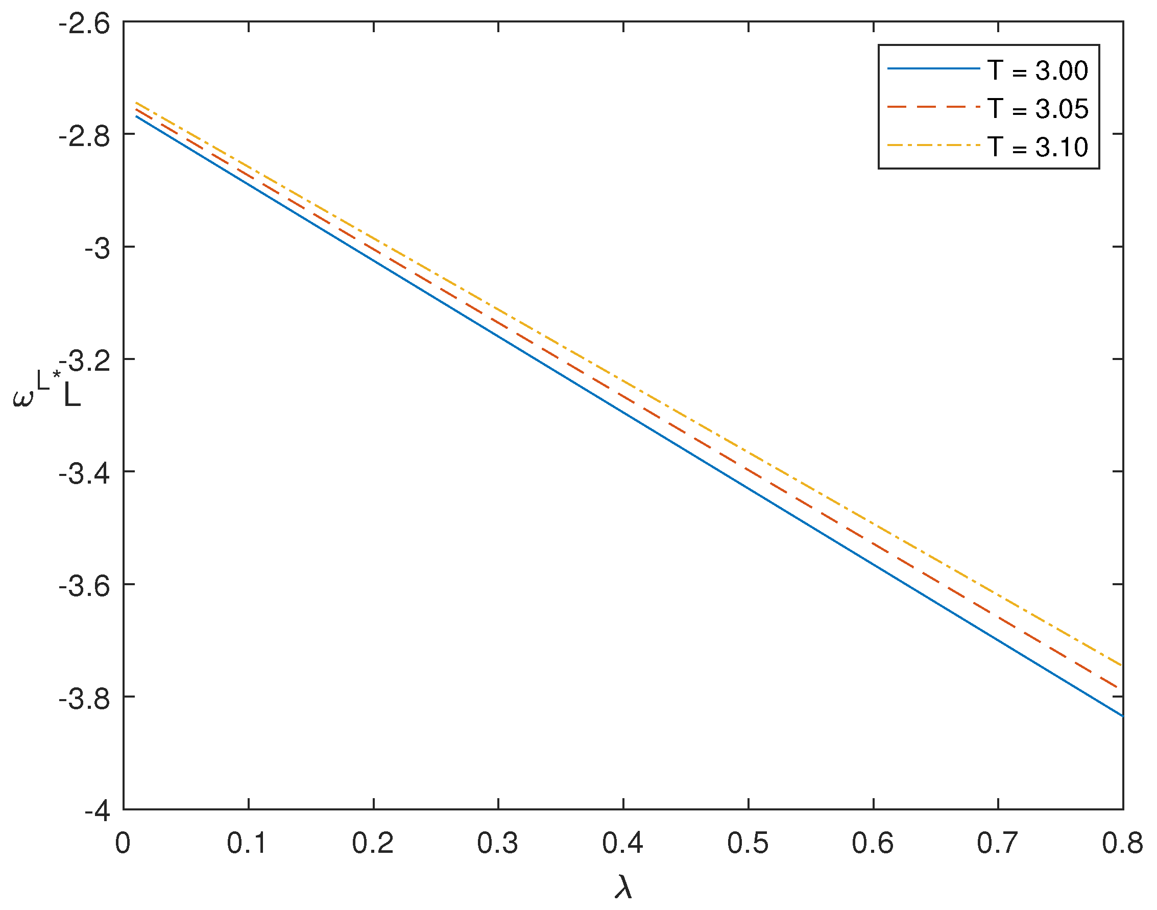
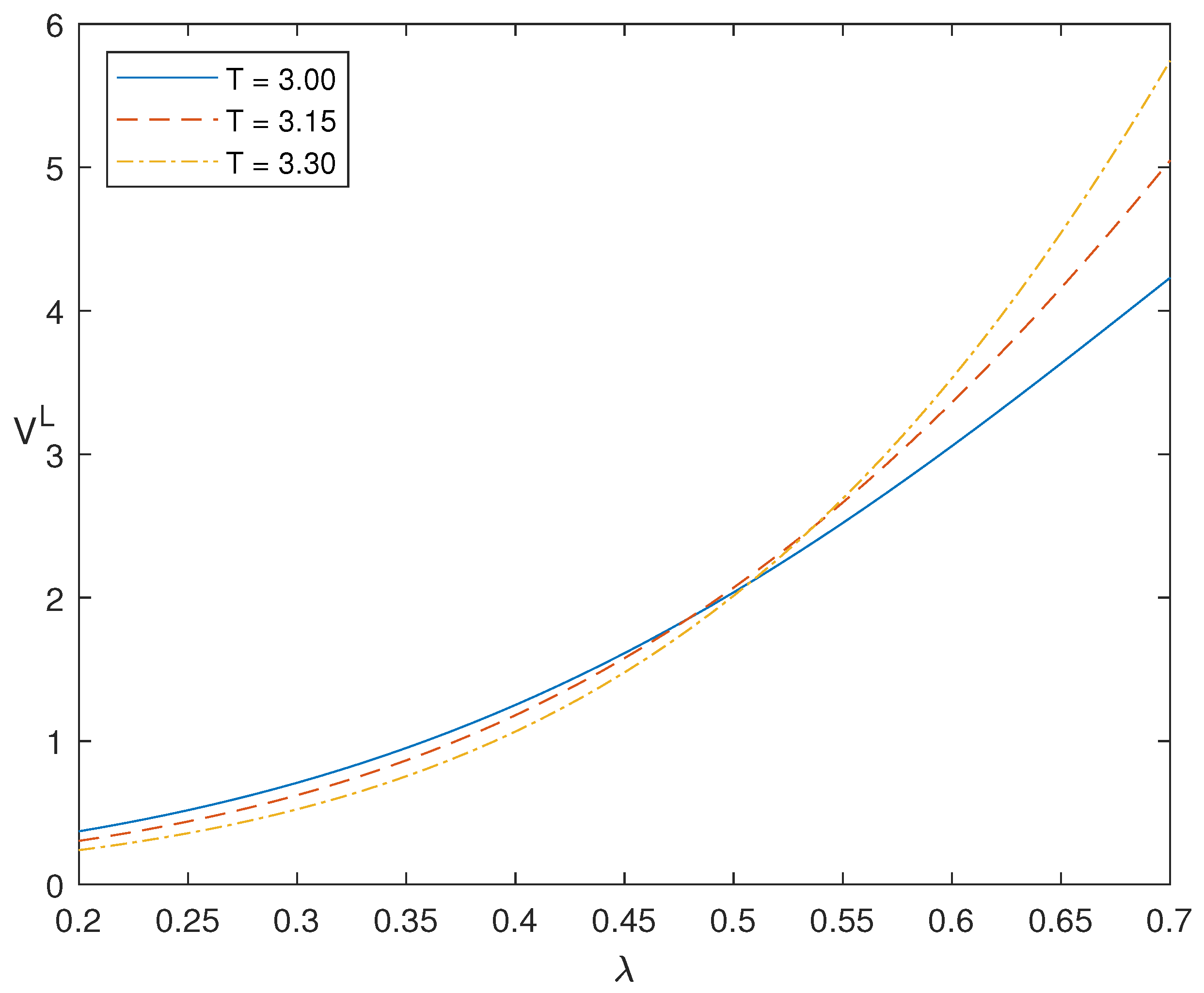
When the mortality rate is high, the longevity risk is usually low. Likewise, might be low because the sponsor may not need a lot of longevity bonds to hedge longevity risk. From another aspect, when the mortality rate is high, the price of longevity bond is low, thus might be low, too. To test this point of view, Figure 3 demonstrates the effect of mortality rate on optimal investment strategy . When the mortality rate becomes larger, the investment amount becomes smaller. Figure 3 also shows that with the same , becomes larger with a longer T. A rational explanation is that the DB pension scheme faces higher risks in the long run, so investment amount in the risky bond (in a short position) becomes smaller in order to reduce risk, which is more clear in Figure 4.
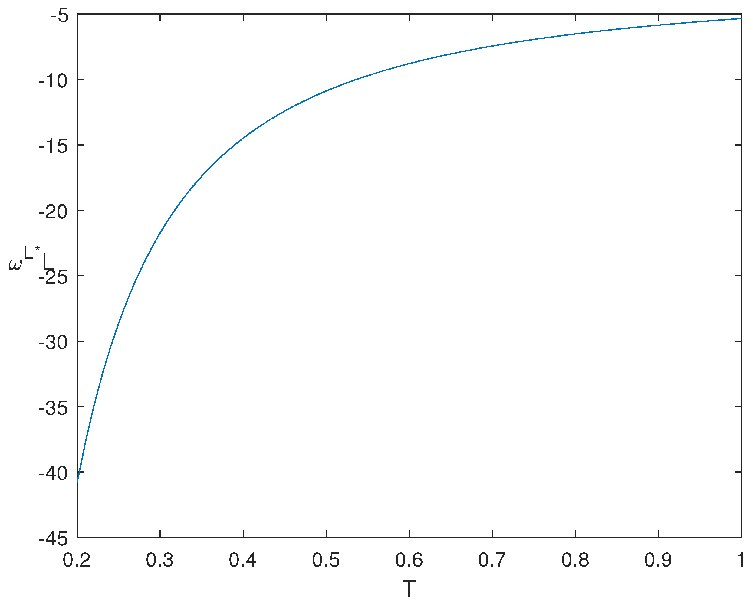
If longevity risk is hedged by the longevity-indexed bond, we may have a lower solvency risk with a lower mortality rate. Figure 5 demonstrates the effect of mortality rate on value function , and it shows that the pension scheme has a lower value function (which means lower solvency risk) with a lower mortality rate (which may cause higher longevity risk). It seems that investments in the longevity bond reduce the solvency risk in a DB pension plan. In addition, Figure 5 also shows that the solvency risk is lower with a smaller in a longer period. It shows that the hedging strategy is more efficient in the long run.
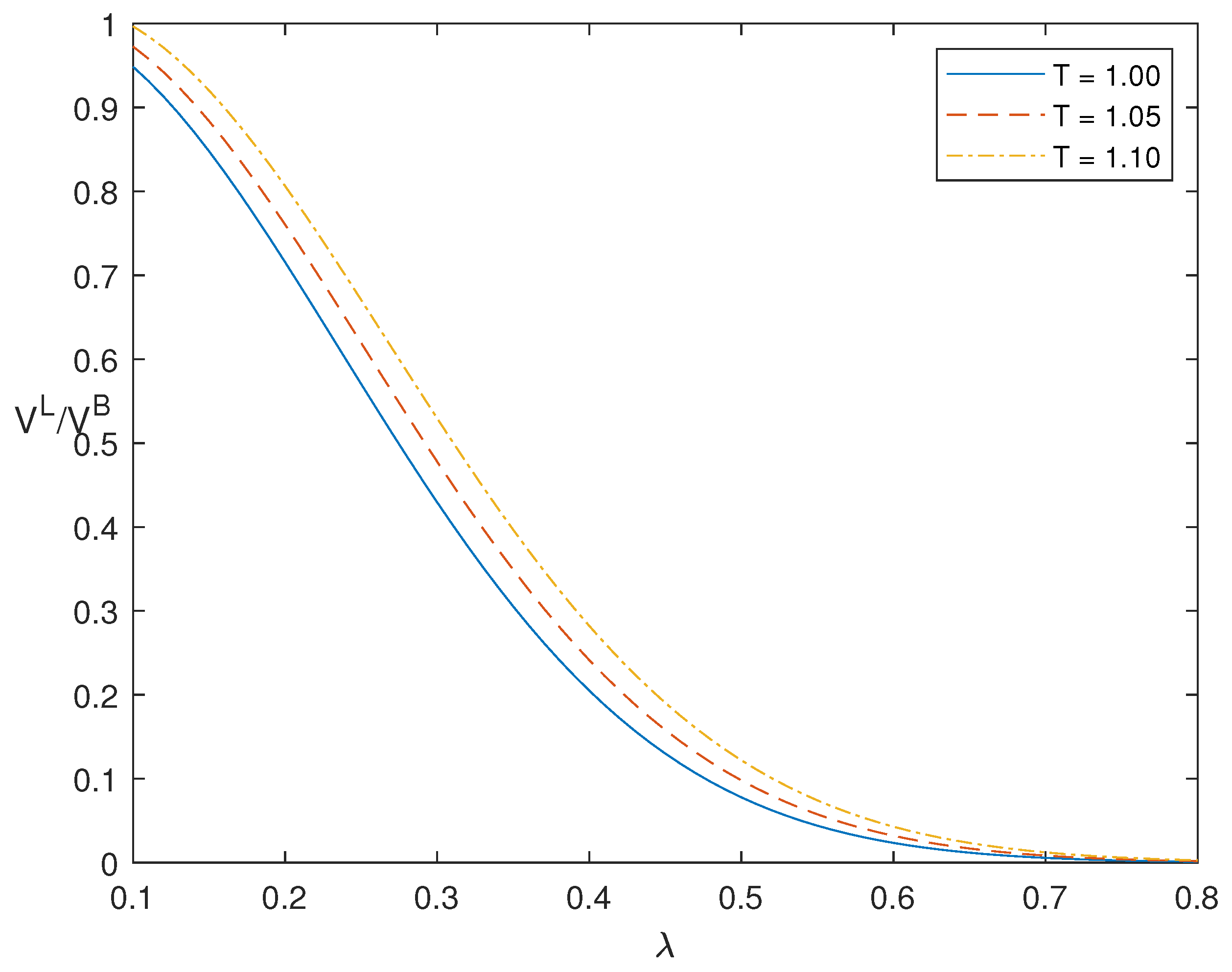
In addition, if longevity risk is reduced by the longevity bond, we may have a lower solvency risk in the market with the longevity bond than that with a normal zero-coupon bond. and denote the value function in Section 3 (with investment in the longevity bond) and Section 4 (with investment in the zero-coupon bond), respectively. To test this, Figure 6 demonstrates the performance of with different values. The ratio is lower than 1 with from to , implying the solvency risk in Section 3 is lower than that in Section 4.
6. Conclusions
This paper investigates, by means of dynamic programming technique, an optimal control problem for an aggregated DB pension plan in a stochastic interest rate framework. The pension sponsor’s objective is to minimize the terminal solvency risk by managing the fund wealth in finite time horizon through a portfolio comprising a longevity-indexed bond and a risk-less asset. The explicit investment policy is derived by solving the corresponding HJB equation. By replacing the longevity-indexed bond with a normal zero-coupon bond, we find that the value function in the market with a longevity bond is lower than that with a zero-coupon bond, i.e., a longevity bond plays a positive role and has a strategic advantage in hedging solvency risk in such DB pension scheme.
It may be significant to consider the benefit process with the influence of mortality rate in the future, which may generate more realistic sample paths of the benefit. Mortality rate may be stochastic. It is also interesting to consider constrained control variable , i.e., short-selling is prohibited, which is consistent with some regulations and risk management policies. This makes the value function unsmooth; thus, the technique of viscosity solutions in the dynamic programming approach might be applied. We leave these two points for future study.
Author Contributions
Conceptualization, J.G.; methodology, J.G. and X.Z.; software, Y.L.; writing—original draft preparation, X.Z.; writing—review and editing, Y.L. All authors have read and agreed to the published version of the manuscript.
Funding
This research was funded by the National Natural Science Foundation of China (No. 12201174, No. 11931018, No. 12271274 and No. 12371468) and the Science and Technology Foundation of Universities in Hebei Province (No. QN2021215).
Data Availability Statement
No new data were created or analyzed in this study.
Conflicts of Interest
The authors declare no conflicts of interest.
Abbreviations
The following abbreviations are used in this manuscript:
| DC | Defined contribution |
| DB | Defined benefit |
| HJB | Hamilton–Jacobi–Bellman |
| SDE | Stochastic differential equation |
| PDE | Partial differential equation |
Appendix A
The proof of Theorem 1.
Substituting Equation (14) into Equations (11) and (12), we determine that the value function V satisfies
with the final value given in Equation (13). The structure of the HJB equation suggests a quadratic form as follows:
where , and are undetermined functions with terminal values , and .
Differentiating Equation (A2), we obtain
where , , are the first- and second-order partial derivatives of with respect to t and r, respectively. Other partial derivatives in Equation (A3) are defined similarly.
Substituting Equation (A3) into Equation (A1) and rearranging it by the order of , and , three PDEs are obtained together with boundary conditions:
since Equation (A1) satisfies for every , and .
To solve Equation (A4), we conjecture that , with terminal conditions and . So we have , and . Substituting , and into Equation (A4), we obtain the following equation:
For convenience, we denote and in Theorem 1 in order to draw comparison with the results given in Section 4. and are given in Equation (17).
The method solving Equation (A4) cannot be used to find an analytical solution of Equation (A5) due to the nonhomogeneous term . By Proposition 2 in the work of Yao et al. (2013), we can derive the solution of Equation (A5) by solving the associated homogeneous PDE in the following:
with ; then, the analytical solution of Equation (A5) is
The analytical solution of Equation (A8) can be derived easily by using the same method as in solving . We try solution , with terminal values and . and are obtained after substituting the first- and second-order derivatives of with respect to t and r into Equation (A8). We denote and , in order to make comparison with results given in Section 4. and are given in Equation (17).
Using Proposition 2, we find that the first equation in Equation (A6) is homogeneous. So it is easy to prove that , since its terminal condition is 0.
References
- Barbarin, Jérôme. 2008. Heath-Jarrow-Morton modelling of longevity bonds and the risk minimization of life insurance portfolios. Insurance: Mathematics and Economics 43: 41–55. [Google Scholar] [CrossRef]
- Bauer, Daniel, Matthias Börger, and Jochen Ruß. 2010. On the pricing of longevity-linked securities. Insurance: Mathematics and Economics 46: 139–49. [Google Scholar] [CrossRef]
- Berstein, Solange, and Marco Morales. 2021. The role of a longevity insurance for defined contribution pension systems. Insurance: Mathematics and Economics 76: 233–40. [Google Scholar] [CrossRef]
- Biagini, Francesca, Thorsten Rheinländer, and Jan Widenmann. 2013. Hedging mortality claims with longevity bonds. ASTIN Bulletin 43: 123–57. [Google Scholar] [CrossRef]
- Blake, David, and Andrew J. G. Cairns. 2021. Longevity risk and capital markets: The 2019–2020 update. Insurance: Mathematics and Economics 99: 395–439. [Google Scholar]
- Blake, David, Andrew J. G. Cairns, and Kevin Dowd. 2006. Living with mortality: Longevity bonds and other mortality-linked securities. British Actuarial Journal 12: 153–97. [Google Scholar] [CrossRef]
- Bravo, Jorge M., and João Pedro Vidal Nunes. 2021. Pricing longevity derivatives via Fourier transforms. Insurance: Mathematics and Economics 96: 81–97. [Google Scholar] [CrossRef]
- Broeders, Dirk, Roel Mehlkopf, and Annick van Ool. 2021. The economics of sharing macro-longevity risk. Insurance: Mathematics and Economics 99: 440–58. [Google Scholar] [CrossRef]
- Chen, An, Hong Li, and Mark B. Schultze. 2023. Optimal longevity risk transfer under asymmetric information. Economic Modelling 120: 106179. [Google Scholar] [CrossRef]
- Cox, Samuel H., Yijia Lin, Ruilin Tian, and Jifeng Yu. 2013. Managing capital market and longevity risks in a defined benefit pension plan. The Journal of Risk and Insurance 80: 585–619. [Google Scholar] [CrossRef]
- Fleming, Wendell H., and Halil Mete Soner. 1993. Controlled Markov Processed and Viscosity Solutions. New York: Springer. [Google Scholar]
- Guan, Guohui, and Zongxia Liang. 2014. Optimal management of DC pension plan in a stochastic interest rate and stochastic volatility framework. Insurance: Mathematics and Economics 57: 58–66. [Google Scholar] [CrossRef]
- Guan, Guohui, Jiaqi Hu, and Zongxia Liang. 2022. Robust equilibrium strategies in a defined benefit pension plan game. Insurance: Mathematics and Economics 106: 193–217. [Google Scholar] [CrossRef]
- Han, Nan-Wei, and Mao-Wei Hung. 2017. Optimal consumption, portfolio, and life insurance policies under interest rate and inflation risks. Insurance: Mathematics and Economics 73: 54–67. [Google Scholar] [CrossRef]
- Josa-Fombellida, Ricardo, and Juan Pablo Rincón-Zapatero. 2004. Optimal risk management in defined benefit stochastic pension funds. Insurance: Mathematics and Economics 34: 489–503. [Google Scholar] [CrossRef]
- Josa-Fombellida, Ricardo, and Juan Pablo Rincón-Zapatero. 2010. Optimal asset allocation for aggregated defined benefit pension funds with stochastic interest rates. European Journal of Operational Research 201: 211–21. [Google Scholar] [CrossRef]
- Kort, Jan, and Michel H. Vellekoop. 2017. Existence of optimal consumption strategies in markets with longevity risk. Insurance: Mathematics and Economics 72: 107–21. [Google Scholar]
- Leung, Melvern, Man Chung Fung, and Colin O’Hare. 2018. A comparative study of pricing approaches for longevity instruments. Insurance: Mathematics and Economics 82: 95–116. [Google Scholar] [CrossRef]
- Liang, Xiaoqing, Lihua Bai, and Junyi Guo. 2014. Optimal time-consistent portfolio and contribution selection for defined benefit pension schemes under mean-variance criterion. The ANZIAM Journal 56: 66–90. [Google Scholar] [CrossRef]
- Liu, Zilan, Huanying Zhang, and Lei He. 2023. Optimal assets allocation and benefit adjustment strategy with longevity risk for target benefit pension plans. Journal of Industrial and Management Optimization 19: 3931–51. [Google Scholar] [CrossRef]
- Menoncin, Francesco. 2008. The role of longevity bonds in optimal portfolios. Insurance: Mathematics and Economics 42: 343–58. [Google Scholar] [CrossRef]
- Menoncin, Francesco, and Luca Regis. 2017. Longevity-linked assets and pre-retirement consumption/portfolio decisions. Insurance: Mathematics and Economics 76: 75–86. [Google Scholar] [CrossRef]
- Ng, Kenneth Tsz Hin, and Wing Fung Chong. 2023. Optimal investment in defined contribution pension schemes with forward utility preferences. Insurance: Mathematics and Economics 114: 192–211. [Google Scholar] [CrossRef]
- Rong, Ximin, Cheng Tao, and Hui Zhao. 2023. Target benefit pension plan with longevity risk and intergenerational equity. ASTIN Bulletin 53: 84–103. [Google Scholar] [CrossRef]
- Wills, Samuel, and Michael Sherris. 2010. Securitization, structuring and pricing of longevity risk. Insurance: Mathematics and Economics 46: 173–85. [Google Scholar] [CrossRef]
- Yao, Haixiang, Zhou Yang, and Ping Chen. 2013. Markowitz’s mean-variance defined contribution pension fund management under inflation: A continuous-time model. Insurance: Mathematics and Economics 53: 851–63. [Google Scholar] [CrossRef]
- Yong, Jiongmin, and Xun Yu Zhou. 1999. Stochastic Controls: Hamiltonian Systems and HJB Equations. New York: Springer. [Google Scholar]
- Zhang, Xiaoyi. 2018. The role of longevity bond in DC pension plan during both accumulation and decumulation phases. Chinese Journal of Engineering Mathematics 37: 347–69. [Google Scholar]
- Zhu, Nan, and Daniel Bauer. 2014. A cautionary note on natural hedging of longevity risk. North American Actuarial Journal 18: 104–15. [Google Scholar] [CrossRef]
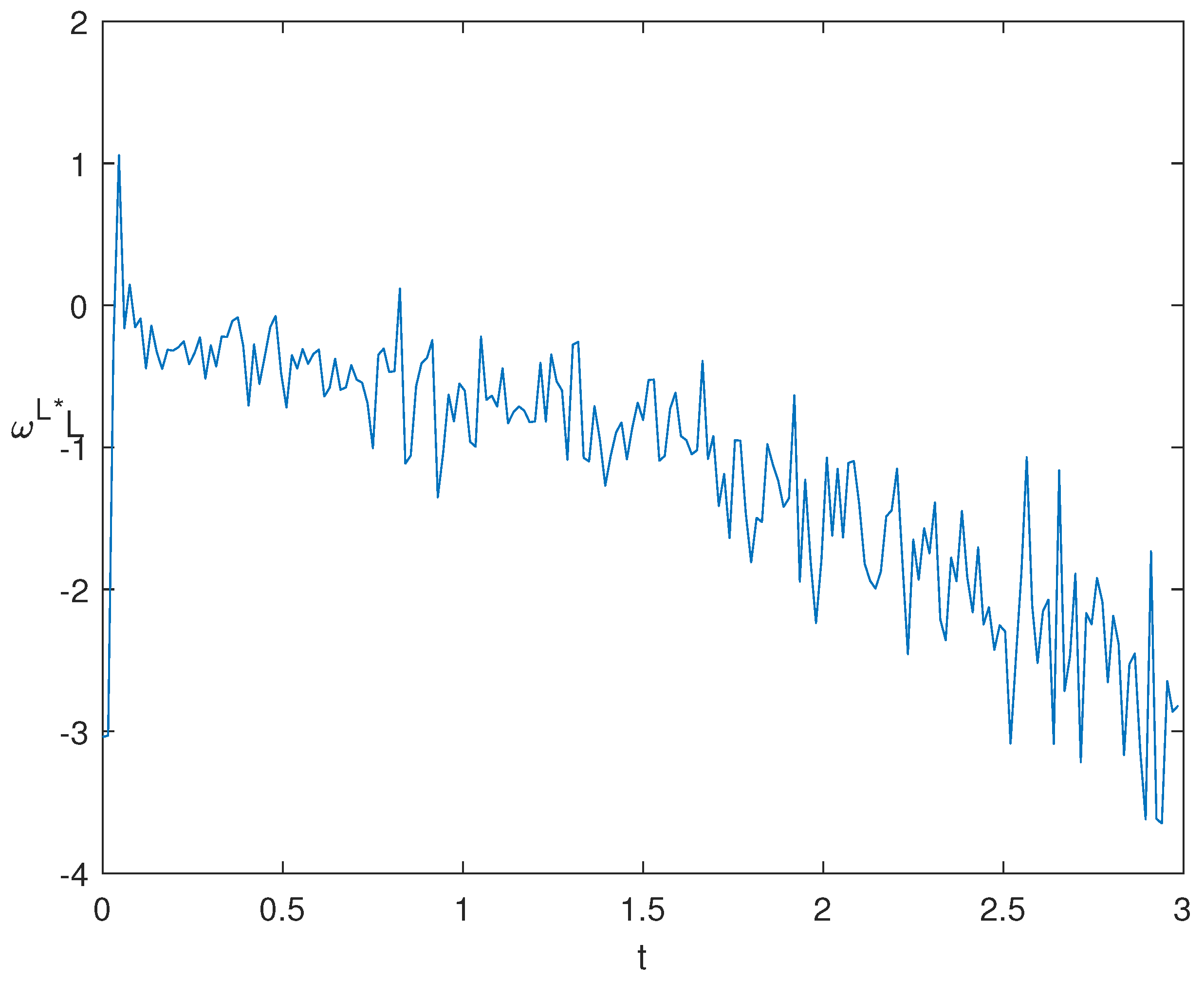
Figure 1.
A possible path of the optimal investment strategy .

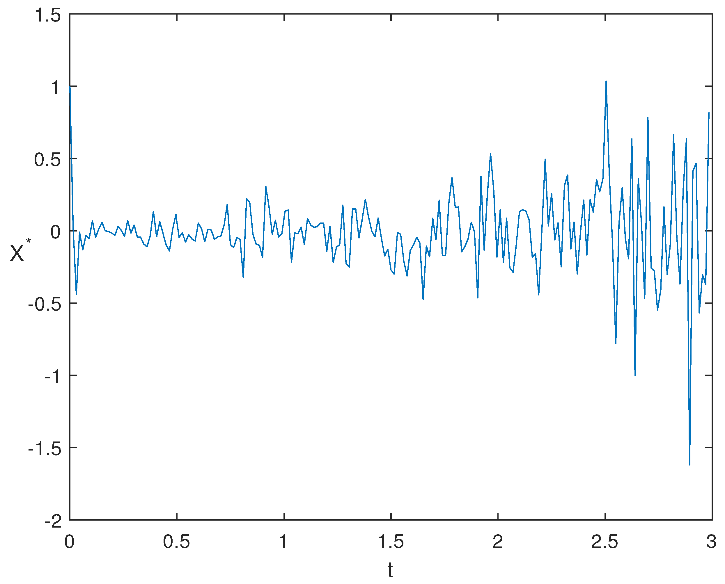
Figure 2.
A possible path of .

Figure 3.
This figure plots the relationship between mortality rate and optimal investment strategy with different T.
Figure 3.
This figure plots the relationship between mortality rate and optimal investment strategy with different T.

Figure 4.
This figure plots the relationship between terminal time T and optimal investment strategy with .
Figure 4.
This figure plots the relationship between terminal time T and optimal investment strategy with .

Figure 5.
This figure plots the relationship between mortality rate and value function with different terminal time T.
Figure 5.
This figure plots the relationship between mortality rate and value function with different terminal time T.

Figure 6.
This figure plots the relationship between mortality rate and ratio with different terminal time T.
Figure 6.
This figure plots the relationship between mortality rate and ratio with different terminal time T.


Table 1.
Parameters of the model.
| a | b | |||||||||
|---|---|---|---|---|---|---|---|---|---|---|
| 1 | 1 | 0.5 | 0.1 | 0.3 | 0.5 | −0.5 | 0.3 | 0.0015 | 0.03 | 0.05 |
Disclaimer/Publisher’s Note: The statements, opinions and data contained in all publications are solely those of the individual author(s) and contributor(s) and not of MDPI and/or the editor(s). MDPI and/or the editor(s) disclaim responsibility for any injury to people or property resulting from any ideas, methods, instructions or products referred to in the content. |
© 2024 by the authors. Licensee MDPI, Basel, Switzerland. This article is an open access article distributed under the terms and conditions of the Creative Commons Attribution (CC BY) license (https://creativecommons.org/licenses/by/4.0/).
Share and Cite
MDPI and ACS Style
Zhang, X.; Li, Y.; Guo, J. The Role of Longevity-Indexed Bond in Risk Management of Aggregated Defined Benefit Pension Scheme. Risks 2024, 12, 49. https://doi.org/10.3390/risks12030049
AMA Style
Zhang X, Li Y, Guo J. The Role of Longevity-Indexed Bond in Risk Management of Aggregated Defined Benefit Pension Scheme. Risks. 2024; 12(3):49. https://doi.org/10.3390/risks12030049
Chicago/Turabian StyleZhang, Xiaoyi, Yanan Li, and Junyi Guo. 2024. "The Role of Longevity-Indexed Bond in Risk Management of Aggregated Defined Benefit Pension Scheme" Risks 12, no. 3: 49. https://doi.org/10.3390/risks12030049
Note that from the first issue of 2016, this journal uses article numbers instead of page numbers. See further details here.