
Bayesian Inference for the Loss Models via Mixture Priors

Department of Mathematics, Towson University, Towson, MD 21252, USA
*
Author to whom correspondence should be addressed.
Risks 2023, 11(9), 156; https://doi.org/10.3390/risks11090156
Submission received: 5 June 2023
/
Revised: 16 August 2023
/
Accepted: 18 August 2023
/
Published: 31 August 2023
Abstract
:Constructing an accurate model for insurance losses is a challenging task. Researchers have developed various methods to model insurance losses, such as composite models. Composite models combine two distributions: one for part of the data with small and high frequencies and the other for large values with low frequencies. The purpose of this article is to consider a mixture of prior distributions for exponential–Pareto and inverse-gamma–Pareto composite models. The general formulas for the posterior distribution and the Bayes estimator of the support parameter are derived. It is shown that the posterior distribution is a mixture of individual posterior distributions. Analytic results and Bayesian inference based on the proposed mixture prior distribution approach are provided. Simulation studies reveal that the Bayes estimator with a mixture distribution outperforms the Bayes estimator without a mixture distribution and the ML estimator regarding their accuracies. Based on the proposed method, the insurance losses from natural events, such as floods from 2000 to 2019 in the USA, are considered. As a measure of goodness-of-fit, the Bayes factor is used to choose the best-fitted model.
1. Introduction
Constructing an accurate loss model for insurance loss is one of the essential topics in actuarial science. Insurance industry data have unique properties. They have a high frequency for small losses and very few significant losses. A traditional distribution, such as normal and others, cannot describe insurance data skewness and fat-tailed properties. Therefore, many researchers explored the other distributions to fit the insurance loss data better. The class of composite distributions is one of them. A composite distribution combines a typical distribution, such as exponential, inverse-gamma, Weibull, and log-normal, for the data with slight losses and the Pareto distribution with extreme losses but low frequencies.
Klugman et al. (2012) provided a detailed discussion on modeling datasets in actuarial science. Teodorescu and Vernic (2006) considered the exponential–Pareto composite model and derive the maximum likelihood estimator for the support parameter . Preda and Ciumara (2006) employed the composite models Weibull–Pareto and log-normal–Pareto to model insurance losses. These models have two parameters: one is the support parameter and another is the shape parameter . In the article, they developed algorithms to find and compare the maximum likelihood estimates for two unknown parameters. Cooray and Cheng (2013) estimated the parameters of the log-normal–Pareto composite distribution by using Bayesian methods with both Jeffreys and conjugate priors. They used MCMC methods rather than developing closed mathematical formulas. Scollnik and Sun (2012) developed several composite Weibull–Pareto models and suggested using them in different situations. Aminzadeh and Deng (2017) reconsidered the composite exponential–Pareto distribution and provided the Bayesian estimate of the via inverse-gamma as the prior distribution. Aminzadeh and Deng (2019) developed an inverse-gamma–Pareto composite distribution to model insurance losses and provided Bayesian inference based on gamma prior distribution. Deng and Aminzadeh (2019) revisited the Weibull–Pareto composite model and derived the Bayesian inference for the model. In Deng and Aminzadeh (2019), both inverse-gamma (IG) and gamma priors were employed to find Bayes estimates of the support parameter of and the shape parameter . They also confirmed via simulation studies that the Bayes estimates of the parameters consistently outperform MLEs in all cases. Bakar et al. (2015) develop several new composite models on the Weibull distribution for heavy-tailed insurance loss data. These models are fitted to two real insurance loss data and their goodness-of-fit is tested.
Mixture distributions have applications in many fields, including insurance, actuarial science, and risk management. Klugman et al. (2012) discussed why mixture distributions have broad applications in the actuarial science field. Miljkovic and Grün (2016) used the mixture distributions to model insurance losses. They compared the mixture model with composite models for Danish Fire data and pointed out that it is better than composite models. Bhati et al. (2019) used a mixture of the Pareto and log-gamma distributions to model the heavy-tailed losses.
Abdul Majid and Ibrahim (2021a) analyzed composite Pareto models for Malaysian household income data. The parameter estimation uses numerical methods based on maximum pseudo-likelihood. The conclusion is that the log-normal–Pareto (II) model provides the best fit compared to other models. Abdul Majid and Ibrahim (2021b) proposed a Bayesian approach to composite Pareto models that involves prior distribution on the proportion of data coming from the Pareto distribution instead of assuming the prior distribution on the threshold . They concluded that a uniform prior on the proportion approach is less biased than the point estimates determined when using a uniform prior on the threshold. Deng et al. (2021) provided an analytical Bayesian approach to derive estimators of the log-normal–Pareto composite distribution parameters based on the selected priors. The article compared exponential–Pareto, inverse-gamma–Pareto, and log-normal–Pareto as candidate models for data on natural hazards from 1900 to 2016 in the USA. The conclusion is that the log-normal–Pareto distribution provides the best fit.
To model large losses, the Pareto distribution is the distribution favored by practitioners and researchers for modeling heavy-tailed financial data. However, when losses consist of smaller values with high frequencies and larger losses with low frequencies, the log-normal or the Weibull distributions are preferred. Nevertheless, no ordinary distribution provides an acceptable fit for both small and large losses. On the one hand, as mentioned by Dominicy and Sinner (2017), the Pareto fits the tail well, but on the other hand, log-normal, Weibull, and inverse-gamma produce an overall good fit but fit the tail badly. The purpose of using composite distributions is to overcome the dilemma. Saleem (2010) considers type-I mixtures of the members of a subclass of the one-parameter exponential family distributions, such as exponential, Rayleigh, Pareto, Burr type XII, and power function distributions for censored data. The article provides Bayes estimators of parameters using ML, as well as uniform and Jeffreys priors. To our knowledge, the mixture of the priors’ approach has not been considered in the literature for composite distributions. The proposed method in the current article considers two composite distributions. The mixture prior method is based on gamma and inverse-gamma priors, which are good candidates for the positive threshold parameter . Furthermore, we propose a data-driven approach to compute optimal values for hyperparameters. For a real dataset where a selected “true” value for (unlike in simulations) is not available, we propose using the MLE of along with the characteristics of the prior distribution to assign optimal values for the hyperparameter values.
In this article, we apply the Bayesian method to the composite models using a mixture of prior distributions instead of a single prior distribution for . The motivation comes from the natural loss of data over many years due to many factors, such as floods, fires, storms, and earthquakes. Each of them should have a distribution with its parameters. Therefore, the mixture distribution describes the overall distribution. The organization of the article is as follows. Section 2 discusses the general mixture prior, the general mixture posterior, and the general predictive distributions with the risk measures. Section 3 provides the formulas for Bayes estimators of via the mixture prior distribution approach for both exponential–Pareto and gamma–Pareto composite models. Section 4 summarizes simulation studies based on equality-weighted mixture distributions and compares the accuracy of different methods. Section 5 analyzes the natural disaster loss data to illustrate the computations involved and identifies the best model using the Bayes factor as a goodness-of-fit measure.
2. Mixture Distribution
Definition 1.
A random variable Z is a K-point mixture of the random variables if its cdf is given by
where and
Therefore, a mixture distribution density is given by
The steps to derive the posterior distribution of the random variables with a mixture prior distribution are as follows:
Let be a random sample from the distribution with a parameter . The likelihood function L() can be written as follows:
Let the prior distribution of the parameter be a K-point mixture distribution with the density function given by
where all , and , and
Therefore, the joint distribution of and X is
where belong to the same class of distributions. For example, all could be Pareto, gamma, or normal. The marginal distribution of X is given by
The posterior distribution of is
For now, consider only the prior distribution and denote the corresponding joint distribution as , then
Let us denote the corresponding marginal distribution of X as , then
Therefore, the corresponding posterior distribution is
which implies
Using (2) and (1), the posterior distribution, based on the K-point mixture prior , (, is given by
where
because, . Therefore, . Hence, the form of the posterior pdf in (3) confirms that the posterior distribution based on a mixture prior distribution is also a mixture distribution of the individual posterior distributions.
Now, we consider the predictive distribution of Y, given X. Let y denote a future realization of the random variable Y. We assume that , which is the case for the composite models.
The predictive density of y, given x, is formulated as follows:
Using (3) and (4), and noting that , we obtain
Recall that we have already shown . Therefore, the predictive distribution of the mixture prior distribution is also the mixture distribution of the individual predictive distributions.
2.1. Example: Exponential with a Mixture of Gamma Distributions
Let be independent identically distributed (iid) random variables from the exponential distribution with parameter . The density function is given by
and the likelihood function is
Let the prior distribution of be in the class of gamma distributions with parameters and . Then the mixture prior distribution is
Therefore, the joint distribution is given by
Hence, the marginal distribution of X is given by
The integrand in RHS of (6) is the kernel of the gamma distribution with parameters and .
Using (5) and (7), the posterior distribution is given by
And after some algebraic manipulations, (8) reduces to
As expected, the RHS of (9) confirms that the posterior distribution is the mixture distribution of the individual posterior distributions.
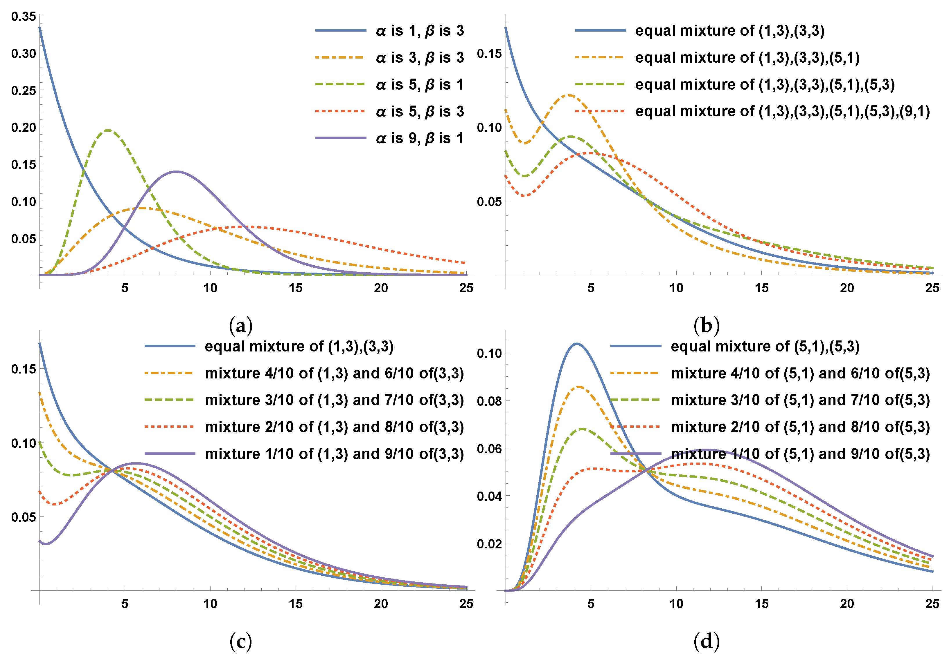
Figure 1a provides graphs for five individual gamma distributions with the shape parameter and the scale parameter . Figure 1b provides graphs for equally weighted mixtures for gamma distributions. Figure 1c provides graphs of mixture gamma distributions with equal weights for two gamma distributions with different shaped parameters and equal scale parameters. Figure 1d provides graphs for the mixture of gamma distributions with unequal weights for gamma distributions with the same parameter shape but different scale parameters. Figure 1b–d confirm that the general shape of the pdf for the mixture distribution is significantly different from that of the pdf for individual gamma distributions in Figure 1a.
3. Bayesian Approach to Composite Models based on the Mixture Prior Distribution
3.1. Bayesian Inference for Composite Exponential–Pareto Based on the Mixture Prior Distribution
Teodorescu and Vernic (2006) considered the exponential–Pareto composite model.
Suppose a random variable X has the pdf defined as a piecewise function,
where
and
The pdf of the exponential distribution with parameter is denoted by , and the pdf of the Pareto distribution with parameters and is denoted by .
Since the pdf of a composite distribution should be a smooth function, the continuity and differentiability conditions on at are necessary. Hence,
As explained in Teodorescu and Vernic (2006), the above equations reduce to
which lead to
Numerical methods via Mathematica for the second equation above, lead to
Since , the normalizing constant c is computed as Therefore, the initial three parameters reduce to only one parameter , and the pdf of the exponential–Pareto distribution is
For , the cdf is
When ,
Therefore, we have the CDF as a piecewise function
To find the quantile through , for , we consider two cases. Since , first consider the case . Solving for , gives Note that for , the first quartile is .
For the case , solving
gives
For the special case , we have 331,596 . In light of the above findings, the quantile function for the exponential–Pareto is
For a random sample from the composite pdf in (10), without loss of generality, assume . The likelihood function can be formulated as
where . To formulate the likelihood function, we assume that, without loss of generality, there is an so that in the ordered sample .
The solution to is the MLE of ,
Note that the Fisher information is
where,
provides the standard deviation of the MLE.
We can see that the MLE requires the correct value of m for its computation. By the assumption, , the algorithm below goes through the following steps to compute .
- Get sorted sample observations
- Start with , compute , if , then , otherwise go to step 3.
- Let , compute , if , then , otherwise go to next step.
The above process continues until we identify the correct value for m. Using the correct value of m, can be computed.
Aminzadeh and Deng (2017) developed Bayesian inference for the exponential–Pareto composite model by considering inverse-gamma as the prior distribution for ,
Using (11) and (12), the posterior pdf is
Using the squared-error loss function, the Bayes estimator for is
where and .
It is shown in the article that the Bayes estimator (14) is consistently better than the MLE in regards to accuracy.
Now, consider the mixture prior distribution of inverse-gamma distributions. Let
where the prior distribution is given by
The pdf of the composite model based on the prior is given by
The integrand in the last line of (16) is the kernel of inverse-gamma with parameters and , where and . Therefore,
Using the above result, the posterior distribution is
which reduces to
Furthermore, we have
hence,
Using the above results, the posterior distribution, based on the mixture prior distribution, is
Hence, under the squared-error loss function, the Bayes estimator for is
3.2. Bayesian Inference for the Composite IG–Pareto Based on the Mixture Prior Distribution
Aminzadeh and Deng (2019) developed the composite inverse-gamma–Pareto model as follows:
Suppose X is a random variable with the pdf , where and , respectively, are the pdfs of inverse-gamma and Pareto distributions.
where
and
Recall that the composite pdf should be smooth at . Therefore,
The simultaneous solutions of the above equations, after algebraic manipulations, lead to
where and , which implies The functions on both sides of the above equations are positive and integrable; therefore, the integrals of the functions on a closed interval should be equal. Hence,
Using the gamma function, we obtain
where denotes the incomplete upper gamma function. In light of this result, the above equation reduces to
Mathematica can solve the above equation numerically. We obtain . As a result, we have . To find the value of c, we need (see the definition of the composite pdf above)
which leads to
Note that GR stands for GammaRegularized and is the cdf of inverse-gamma with parameters . Therefore, , which is the first integral above, reduces to . Mathematica can compute the GR function. The above findings reveal that four initial parameters reduce to only one parameter . As a result, the pdf of the IG–Pareto distribution is
and its cdf is given by
The quantile function can be derived similarly to the exponential–Pareto composite distribution. Using the cdf above, we have .
Case 1:
where can be computed via Mathematica.
Case 2:
For the special cases and , using the constant values , , , and Mathematica, we obtain
Suppose is a random sample from the IG–Pareto distribution, without loss of generality, we assume . The likelihood function is
where . For the formulation of the likelihood function, we assume an exists, such that in the sorted sample . The solution to is the MLE for , which is
Using (20), the Fisher information is
As a result, the standard error of the MLE is .
Using the same algorithm in Section 3.1, we identify the correct value, m, and compute .
Aminzadeh and Deng (2019), as a prior distribution for , used gamma( with the pdf
then, the posterior pdf is
The R.H.S. in (21) is the kernel of gamma, and . As a result, the pdf of the posterior is given by
as a result, under the squared-error loss function, the Bayes estimator for is
Now, we derive the Bayes estimator using the mixture prior distribution based on individual gamma priors,
as a result
The pdf of the composite model based on prior is given by
The RHS of the last line in (23) is the kernel of Gamma(, where
Therefore, and
Therefore, the pdf of posterior distribution is
From (24) and (25), we conclude that the posterior distribution for IG–Pareto based on the mixture of gamma priors is
Hence, under the squared-error loss function, the Bayes estimator for is
4. Simulation
4.1. Simulation for Composite Exponential–Pareto
To compare the accuracies of and (with and without a mixture of prior distributions), simulations are conducted using Mathematica. For the same generated sample, the code computes estimators using (), weights For each set of input parameters in the simulation, samples from the composite density (10) are generated.
For a random sample from the composite pdf (10) and without loss of generality, consider the ordered sample . Recall (18),
The following algorithm is used to determine m:
- Start with , check to see if , if yes, then . Otherwise, go to step 2.
- For , if , then , otherwise we consider and continue until we find the correct value for m. The idea is to find the value for m so that . The Mathematica code uses the algorithm to find m and compute .
Selecting hyperparameter values could be challenging. Suppose two experts can provide partial prior information about the hyperparameter values. See, Rufo et al. (2010). The idea with the mixture prior distribution is to incorporate both experts’ opinions to find the Bayes estimate of . In this article, we use the same weights ( for each expert’s opinion and consider two cases when :
It is noted that and , which implies that . It is also noted and , and . From (18), we have
Case 1: In this case, experts are quite sure about the values for and ; therefore, there are only two hyperparameter values that should be selected. We would like the optimal values for . Given values of , Mathematica provides optimal values of via a numerical optimization and the constraints and, .
For example, for , we obtain . Note that unlike in simulation studies, for a real dataset, a selected value for is not available. Hence, we propose a data-driven approach be used to compute . Meaning, the equation along with the above optimization command provide values for and .
Table 1a reveals that by selecting the hyperparameters, as described above, the mixture prior approach gives a more accurate Bayes estimate, as the average squared-error = ASE (Bayes) = is smaller than its counterpart that does not use a mixture prior. For example, for , we obtain . We can see that the smallest ASE values = 0.45027 and 0.41351, corresponding to the optimal set of hyperparameter values of n = 30,100, respectively. Also, comparing Table 1a with Table 1b, it is clear that both Bayes estimators (with and without the mixture prior) outperform MLE with regard to their accuracies, as is much smaller than . Boldface numbers in tables indicate the optimal values.
Case 2: In this case, experts are pretty sure about the values for and , and they would like the optimal values for . Given values of , Mathematica provides optimal values of via a numerical optimization and the constraint .
For example, for , we obtain Similar to case 2, to compute , we use in the above optimization command to find .
Like the previous case, Table 2a confirms that by selecting the hyperparameters, as described above, the mixture prior approach provides a more accurate Bayes estimate, as ASE (Bayes) = is smaller than its counterpart that does not use a mixture prior. For example, for , we obtain . Again, the smallest ASE values = 0.26801 and 0.24191, corresponding to the optimal hyperparameter values of n = 30 and 100, respectively. Also, comparing Table 2a with Table 2b, in this case, both Bayes estimators (with and without the mixture prior) outperform MLE with regard to their accuracies.
4.2. Simulation for Composite Inverse-Gamma–Pareto
Simulations compare similarly to the composite exponential–Pareto model to compare the accuracy of based on with and without mixture prior distributions. For selected values of n and , the hyperparameters () for gamma prior distributions, and weights . The simulation study generates samples from the composite density (19).
Given a random sample from the composite pdf in (19), without loss of generality, consider the ordered sample . Recall the Bayes estimator (26), which uses the mixture gamma prior distributions,
The algorithm described in Section 4.1 determines the value of m. Like the exp–Pareto composite distribution case, we must select the prior distributions’ hyperparameters. We consider the mixture prior distribution with equal weights and . For the prior distribution , and , consider two cases:
Here, , under the assumption , it can be shown that
Table 3a and Table 4a provide simulation results for Cases 1 and 2. Since , and , we have
From (26), we have
Case 1:
For given values of and , Mathematica provides optimal values of via a numerical minimization for , and the constraint . Again, when we have a real dataset, is used in the optimization command below in Mathematica to compute hyperparameters
For example, when , and , the optimal solutions are . When , and , the optimal solutions .
Table 3a reveals that by selecting the hyperparameters, as described above, the mixture prior approach gives a more accurate Bayes estimate, as ASE (Bayes) = is smaller than its counterpart that does not use a mixture prior. For example, for a sample size of , the smallest ASE values = 1.72061 and 1.16326, corresponding to the optimal two sets of hyperparameter values. Also, for a sample size of , the smallest ASE values 1.06654 and 0.91892, corresponding to the optimal two sets of hyperparameter values. In this case, Table 3a,b suggest that both Bayes estimators (with and without mixture prior distributions) outperform MLE.
Case 2:
Given the values of and , Mathematica provides optimal values of via a numerical minimization for and the constraint .
For example, for , and , the optimal solutions are . For , and , the optimal solutions are . Similar to other cases, for real data, along with the above command is used to find hyperparameters
Table 4a reveals that the mixture prior approach gives a more accurate Bayes estimate, as ASE (Bayes) = is smaller than its counterpart that does not use a mixture prior. For example, for a sample size of , the smallest ASE values = 1.85072 and 1.20807, corresponding to the optimal two sets of hyperparameter values. Also, for a sample size of , the smallest ASE values = 1.08946 and 0.96434, corresponding to the optimal two sets of hyperparameter values. Table 4a,b reveal that both Bayes estimators (with and without mixture prior distributions) outperform MLE.
5. Numerical Example
5.1. Data and Basic Descriptive Statistics
This section considers possible models via methods presented in the article for the dataset. The objectives are to find out if using the mixture prior approach in the Bayesian framework provides better results concerning the Bayes estimate of the parameter and to select the best model that fits the data. The insurance losses from natural events, such as floods, are obtained from EM-DAT, the International Disaster Database. EM-DAT contains all natural events worldwide in raw data on the occurrences and effects from 1900 to the present day. “The database is compiled from various sources, including the United Nations agencies, non-governmental organizations, insurance companies, research institutes, and press agencies”. This paper considers flood insurance damage in the USA from 2000 to 2019. EM-DAT also provides the annual average CPI using the base year 2019. To eliminate the effect of inflation, all insurance damage amounts are converted to 2019 dollars.
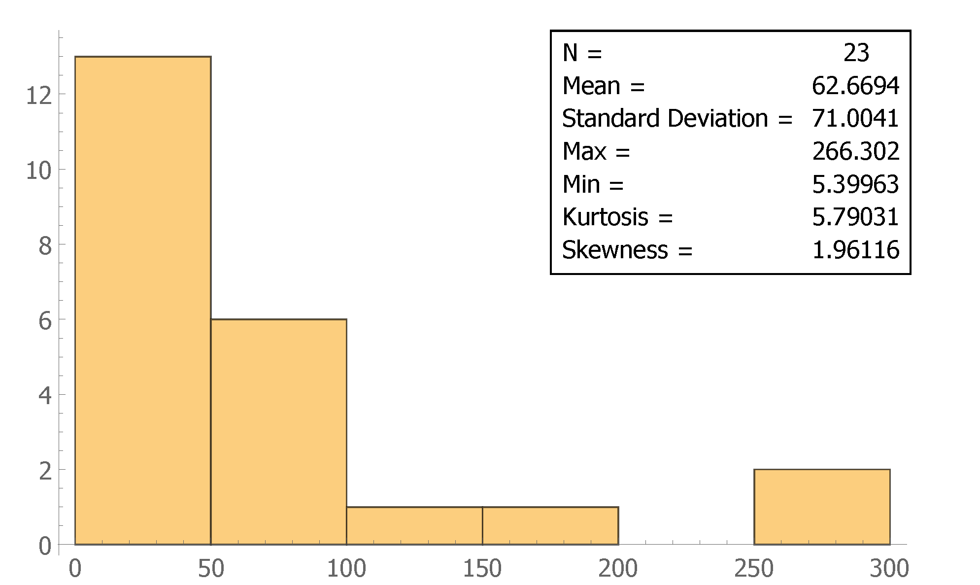
Figure 2 shows the CPI-adjusted (in 2019 dollars) histogram of insurance damage amounts from 2000 to 2019 in the USA. There were 23 recorded insurance losses due to natural event floods in the USA.
Figure 2 provides the frequentist statistics. The average insurance loss due to a natural event storm is = USD 62.6694 million, the minimum loss is USD 5.3996 million, and the maximum loss is USD 266.302 million. The standard deviation is s = USD 71.0041 million, which indicates that the data are widespread. The skewness is 1.96116, which indicates that the data are right-skewed. The kurtosis is 5.79031, which tells us the data have a heavy tail. The histogram also shows the high frequency for small amounts of damage and the low frequency for large amounts of insurance losses. The data represent typical insurance data for which composite models are applicable; see Aminzadeh and Deng (2019). The regular distributions, such as normal and exponential, cannot effectively model the losses.
5.2. Model Selection
Miljkovic and Grün (2016) provide goodness-of-fit measures to determine the appropriateness of the fitted models.
NLL: the negative log-likelihood
NLL is used to compare models with the same number of parameters. NLL corresponds to the model with the minimum value of , among models considered, where is the likelihood function of data, and is the parameter that can be multi-dimensional. The model with a smaller NLL value indicates that the model has a better fit for the data than other models under consideration.
AIC: Akaike’s information criterion
To compare models with different parameter numbers, we consider AIC (Akaike’s information criterion) and BIC (Bayesian information criterion). Both measures penalize the increase in the number of parameters.
Akaike developed AIC,
where q is the number of parameters. As q increases, decreases and 2q becomes larger. It provides the trade-off between the models with different parameters. The model with a smaller AIC value indicates that the model has a better fit for the data than other models under consideration.
BIC: Bayesian information criterion
BIC was proposed by Schwarz and is given by
which also depends on the sample size n. BIC not only penalizes the increase in the number of parameters but also the increase in the sample size. The smallest BIC indicates the best-fitted model among the models under consideration.
5.2.1. Goodness-of-Fit Measures for Maximum Likelihood Method
Table 5 provides the MLE, NLL, AIC, and BIC values for different models. Standard errors of MLEs (see Section 4.1 and Section 4.2) also are listed in the table. For example, when we use the exponential model to fit the insurance flood loss data, there is one unknown parameter . The MLE of based on the exponential model is . Using , the goodness-of-fit measures—NLL, AIC, and BIC—are computed as 118.171, 238.342, and 239.478. Table 5 reveals that based on NLL, AIC, and BIC, among non-composite models (exponential, inverse-gamma) and composite models (exp–Pareto, IG–Pareto), IG–Pareto has the smallest NLL, which is 105.701. Therefore, IG–Pareto is the best-fitted model among all four models for insurance losses due to natural event floods from 2000 to 2019.
5.2.2. Bayesian Inference of IG–Pareto
NLL, AIC, and BIC are criteria for evaluating models estimated by maximum likelihood methods. They may not be suitable for Bayesian model selections. Many researchers proposed the Bayesian approach. Ando (2010) introduced the Bayes factor, originally proposed by Kass and Raftery (1995), among other authors. The logic behind using Bayesian inference for the real data is based on the idea that it provides a more accurate estimator than the ML method, as verified by the simulation studies in Table 1a, Table 2a, Table 3a and Table 4a. The Bayesian estimator based on the mixture prior approach is more accurate than a non-Bayesian method, such as MLE, provided that a data-driven approach is instigated for the hyperparameters.
Bayes factor
The odds of the marginal likelihood of the data, , is given by
where are marginal likelihoods of the dataset corresponding to two models: and . If , it is concluded that is a better-fitted model than . Ando (2010) states, “The Bayes Factor chooses the model with the largest value of marginal likelihood among a set of candidate models”. The following is Jeffreys’ scale of evidence for interpreting the Bayes factor:
- If , negative support for
- If , barely worth mentioning
- If , substantial evidence for
- If , strong evidence for
- If , very strong evidence for
- If , decisive evidence for
The Marginal Likelihood
Let be a random sample with the distribution . Then, the likelihood function is given by
Let be the prior distribution for the parameter , then the marginal likelihood function (PML) is defined by
where , which is the case for composite models, such as exp–Pareto and IG–Pareto considered in this article.
According to Table 5, as IG–Pareto is the best-fitted composite model, going forward, we will consider the mixture prior approach as discussed in the previous sections and apply it to the IG–Pareto composite model. From (20)
where and m is a positive integer, such as . Let gamma( be the prior distribution with the pdf
and . The marginal likelihood function (PML) is
where denotes the gamma function evaluated at A. Now, consider the mixture distribution of gamma priors and , with equal weights .
and let . We can see that, given the mixture prior, the PML is represented as:
As mentioned, selecting the hyperparameters is challenging. The expected value and variance for are given as follows:
To find the optimal values of the hyperparameters and , we propose minimizing the variance under the constraint . Substituting into the variance formula, we have . Therefore, the smaller the , the smaller the variance. The variance is an increasing function concerning the parameter . Note that the coefficient of variation is . Since we do not know the "real" value of , as in the simulation section, we replace with its MLE . Table 6 provides PML values for the selected models ( with and 50, and the corresponding and . It is clear that the smaller the variance, the better the model. For example, the Bayes factor of vs. is . is about times as likely as .
Table 6 also provides PML values based on the mixture prior distribution when and weights . The same Mathematica code as in the simulation section computes the hyperparameter values, assuming the “true” parameter value of theta is = 49.3097.
Recall the expected value and variance for under the assumptions , and , are
Using the Mathematica code below, we find optimal for given (see Case 1 in Section 4.2).
Using the Mathematica code below, we find optimal for given (see Case 2 in Section 4.2).
Table 6 provides the PML values and the Bayesian estimates of the support parameter . We note that the model based on the mixture prior outperforms the models without the mixture prior distribution. The model -based equal-weight mixture of and provides the maximum PML value, which is . Model , with an equal-weight mixture of and , provides the second largest PML value, which is . For example, the Bayes factor of vs. is . Therefore is about times as likely as . Based on Jeffreys’ scale evidence, we have strong evidence for (that it fits the data).
Table 7 summarizes the Bayes factors for Models to , which we discussed in Table 6. It can clearly be seen that M6 outperforms all other models due to Bayes factor 1 for , and M5 is the second best since Bayes factor 1 for . Hence, the model with the mixture prior outperforms the model without the mixture prior. The Bayes factor is denoted as in Table 7.
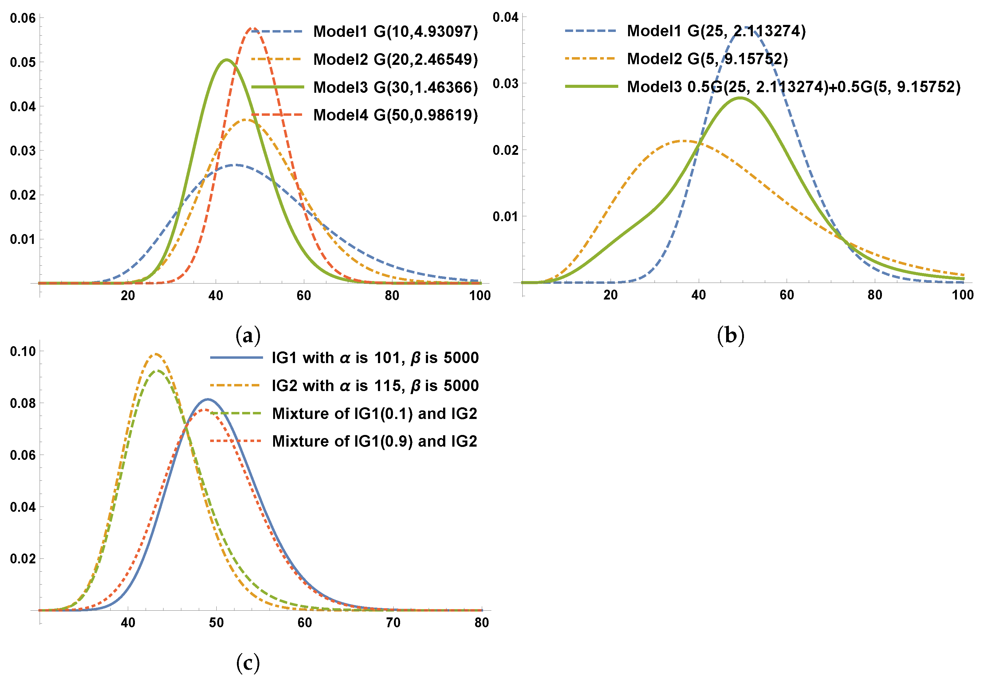
Figure 3 presents the virtual presentation of the gamma priors and the gamma mixture priors to the IG–Pareto composite model in Table 6. Figure 3a shows gamma priors corresponding to to . When the shape parameter increases, the shapes of the curves become more symmetric and bell-shaped; Figure 3b corresponds to ; the equal weight mixture of two gamma priors shows a bimodal shape; even one mode around 28 is not significantly recognized. Figure 3c corresponds to . The equal-weight mixture of two gamma priors clearly shows a bimodal shape.
Table 8 compares the models with the optimal mixture prior () and without the optimal mixture prior (). Note that in the selection of hyperparameters for , we do not minimize the variance. We only ensure the mean equation
is satisfied.
Since the “true” value of is unknown, as mentioned before, we use its MLE = 49.3097. Therefore, for given ,and , we have
which leads to . Also, for the given , and , we have
which leads to .
Table 8 reveals that the models with the optimal mixture prior are better than those without the optimal mixture prior. For example, the Bayes factor () = 5.0458. The model with the optimal mixture prior, , is about 504.58% as likely as the model without the optimal mixture prior, .
The value at risk, Klugman et al. (2012), is an important and standard risk measure in the insurance industry. VaR is the capital required at a higher probability p to ensure the company will not go bankrupt.
The , or an upper limit prediction for a future value y, can be obtained via the predictive density . Aminzadeh and Deng (2019) provide the predictive density for the IG–Pareto composite model based on only one gamma prior distribution, as
where
and
denotes the cdf of gamma and denotes the cdf of gamma, where
The above results can be extended to the mixture of two gamma prior distributions. Recall from Section 2.1,
Therefore, for the case, based on (27), we have
and can be defined via (27) using the corresponding .
The last column of Table 6 for models to provides VaR values, which are found using the predictive density (28),
and Mathematica. The values tell us how much the company should reserve under each model to avoid bankruptcy at the 95% confidence level. For example, if we use model , we should reserve USD million to avoid bankruptcy at the 95% confidence level.
6. Conclusions
This article considers the class of composite models. We are interested in exploring the Bayesian estimates of the threshold parameter , which separates the small losses with high frequencies and significant losses with low frequencies. Two composite models, exp–Pareto and IG–Pareto, are considered as examples. The prior distribution for parameter uses a mixture of prior distributions. We verify that, in general, the posterior distribution is a mixture of individual posterior distributions. For each composite model considered in the article, the general formula of the Bayes estimator of is derived based on the mean squared error loss function.
Simulation results compare the accuracies of using with and without mixture prior distributions. Also, the accuracy of is compared to the Bayes estimates. For both exp–Pareto and IG–Pareto models, respectively, methods for choosing the optimal hyperparameter (, () values, are proposed. The proposed method is data-driven, as it uses the MLE of based on real data to compute optimal values for hyperparameters. Simulations reveal that the Bayesian estimator with the mixture prior distribution is more accurate than the Bayesian estimator without the mixture prior distribution. Also, both Bayes estimators are more accurate than MLE.
For an illustration of computations involved in the proposed methods, the insurance losses in the USA from 2000 to 2019 due to natural event floods are considered and downloaded from EM-DAT, the International Disaster Database. In order to eliminate the effect of inflation, all insurance damage amounts are converted to 2019 dollars. Based on NLL, AIC, and BIC measures, the conclusion is that IG–Pareto provides the best fit, which leads us to apply the Bayesian method to the IG–Pareto composite model. We have shown that the IG–Pareto model with the mixture gamma prior distribution most optimally fits the data based on the optimal hyperparameter value. For the comparison of Bayesian models, the Bayes factor is used.
Potential future research would involve extending the mixture prior approach to other composite distributions, such as log-normal–Pareto and Rayleigh-Pareto. Furthermore, the mixture prior approach can be investigated for composite models that involve more than two distributions. For example, consider Pareto for the right tail of data with very large losses, a non-heavy tail distribution for small losses in the data, and another distribution that models moderate losses in the center of data.
Author Contributions
Conceptualization, M.D. and M.S.A.; Methodology, M.D. and M.S.A.; Software, M.D. and M.S.A.; Validation, M.S.A.; Formal analysis, M.D. and M.S.A.; Investigations, M.D. and M.S.A.; Resources, M.D. and M.S.A.; Data curation, M.D.; writing—original draft preparation, M.D. and M.S.A.; writing—review and editing, M.D. and M.S.A.; visualization, M.D. and M.S.A. All authors have read and agreed to the published version of the manuscript.
Funding
This research received no external funding.
Data Availability Statement
Not applicable.
Acknowledgments
The authors are grateful for the invaluable time and suggestions of the editors and reviewers to enhance the presentation of the article.
Conflicts of Interest
The authors declare no conflict of interest.
References
- Abdul Majid, Muhammad Hilmi, and Kamarulzaman Ibrahim. 2021a. Composite Pareto Distributions for Modeling Household Income Distribution in Malaysia. Sains Malaysiana 50: 2047–58. [Google Scholar] [CrossRef]
- Abdul Majid, Muhammad Hilmi, and Kamarulzaman Ibrahim. 2021b. On Bayesian approach to composite Pareto models. PLoS ONE 16: e0257762. [Google Scholar] [CrossRef] [PubMed]
- Aminzadeh, Mostafa S., and Min Deng. 2017. Bayesian Predictive Modeling for Exponential-Pareto Composite Distribution. Variance 12: 59–68. [Google Scholar]
- Aminzadeh, Mostafa S., and Min Deng. 2019. Bayesian Predictive Modeling for Inverse Gamma-Pareto Composite Distribution. Communications In Statistics, Theory, and Methods 48: 1938–54. [Google Scholar] [CrossRef]
- Ando, Tomohiro. 2010. Bayesian Model Selection and Statistical Modeling. Orange: Chapman & Hall/CRC. [Google Scholar]
- Bakar, S. A. Abu, Nor A. Hamzah, Mastoureh Maghsoudi, and Saralees Nadarajah. 2015. Modeling loss data using composite models. Insurance: Mathematics and Economics 61: 146–54. [Google Scholar]
- Bhati, Deepesh, Enrique Calderín-Ojeda, and Mareeswaran Meenakshi. 2019. A new heavy-tailed class of distributions which includes the Pareto. Risks 7: 99. [Google Scholar] [CrossRef]
- Cooray, Kahadawala, and Chin-I. Cheng. 2013. Bayesian Estimators of the Lognormal-Pareto Composite Distribution. Scandinavian Actuarial Journal 2015: 500–15. [Google Scholar] [CrossRef]
- Deng, Min, and Mostafa S. Aminzadeh. 2019. Bayesian predictive analysis for Weibull-Pareto composite model with an application to insurance data. Communications in Statistics-Simulation and Computation 51: 2683–709. [Google Scholar] [CrossRef]
- Deng, Min, Mostafa S. Aminzadeh, and Min Ji. 2021. Bayesian Predictive Analysis of Natural Disaster Losses. Risks 9: 12. [Google Scholar] [CrossRef]
- Dominicy, Yves, and Corinne Sinner. 2017. Distributions and composite models for size-type data. Advances in Statistical Methodologies and Their Application to Real Problems 159. [Google Scholar] [CrossRef]
- Kass, Robert E., and Adrian E. Raftery. 1995. Bayes factors. Journal of the American Statistical Association 90: 773–95. [Google Scholar] [CrossRef]
- Klugman, Stuart A., Harry H. Panjer, and Gordon E. Willmot. 2012. Loss Models from Data to Decisions, 3rd ed. New York: John Wiley. [Google Scholar]
- Miljkovic, Tatjana, and Bettina Grün. 2016. Modeling loss data using mixtures of distributions. Insurance Mathematics, and Economics 70: 387–96. [Google Scholar] [CrossRef]
- Preda, Vasile, and Roxana Ciumara. 2006. On Composite Models: Weibull-Pareto and Lognormal-Pareto—A comparative Study. Romanian Journal of Economic Forecasting 8: 32–46. [Google Scholar]
- Rufo, María Jesús, Carlos. J. Pérez, and Jacinto Martín. 2010. Merging experts’ opinions: A Bayesian hierarchical model with a mixture of prior distributions. European Journal of Operational Research 207: 284–89. [Google Scholar] [CrossRef]
- Saleem, Muhammad. 2010. Bayesian Analysis of Mixture Distributions. Ph.D. thesis, Quaid-i-Azam University Islamabad, Islamabad, Pakistan. Available online: http://prr.hec.gov.pk/jspui/bitstream/123456789/1430/1/824S.pdf (accessed on 1 August 2023).
- Scollnik, David P. M., and Chenchen Sun. 2012. Modeling with Weibull-Pareto Models. North American Actuarial Journal 16: 260–72. [Google Scholar] [CrossRef]
- Teodorescu, Sandra, and Raluca Vernic. 2006. A composite Exponential-Pareto distribution. The Annals of the “Ovidius” University of Constanta, Mathematics Series 14: 99–108. [Google Scholar]
Figure 1.
Comparison of non-mixture gamma with mixture gamma distributions. (a) Gamma distributions with different parameters. (b) Equally weighted mixture gamma distributions. (c) Unequally weighted mixture of two gamma distributions with different shapes and the same scale. (d) Unequally weighted mixture of two gamma distributions with the same shape and different scales.

Figure 2.
Histogram of insurance damage from 2000 to 2019 in 2019 USD dollars.

Figure 3.
The gamma distribution and the mixture gamma distribution of the prior distribution for the IG–Pareto composite models corresponding to Table 6. (a) Gamma distribution of the prior distribution for the IG–Pareto with different shapes and sizes. (b) The mixture gamma distribution of the prior distribution for the IG–Pareto with different shapes and sizes. (c) The mixture gamma distribution of the prior distribution for the IG–Pareto with different shapes and sizes.


Table 1.
Improved Bayes estimation with hyperparameter selection for mixture priors.
| (a): Comparison of the Bayes estimator without the mixture prior (K = 1) and with the mixture prior (K = 2) when are given | |||||||
| = 5 | |||||||
| K | n | ||||||
| 1 | 30 | 245 | NA | 5.11732 | 0.42551 | ||
| 2 | 30 | 260 | 235 | 52.921 | 48.027 | 5.11662 | 0.42337 |
| 2 | 30 | 260 | 235 | 55 | 46.32143 | 5.12472 | 0.45379 |
| 1 | 100 | 245 | NA | 5.06908 | 0.41555 | ||
| 2 | 100 | 260 | 235 | 52.921 | 48.027 | 5.06875 | 0.41351 |
| 2 | 100 | 260 | 235 | 55 | 46.32143 | 5.09362 | 0.54073 |
| (b): Mean and of MLE of | |||||||
| = 5 | |||||||
| n | |||||||
| 30 | 7.39707 | 4.88656 | |||||
| 100 | 6.09238 | 1.74385 | |||||
Table 2.
Improved Bayes estimation with hyperparameter selection for mixture priors.
| (a): Comparison of the Bayes estimator without the mixture prior (K = 1) and with the mixture prior (K = 2) for given | |||||||
| = 5 | |||||||
| K | n | ||||||
| 1 | 30 | 100 | NA | 5.07243 | 0.27438 | ||
| 2 | 30 | 110 | 98 | 545.312 | 484.727 | 5.07036 | 0.26801 |
| 2 | 30 | 110 | 98 | 560 | 471.651 | 5.07327 | 0.27393 |
| 1 | 100 | 100 | NA | 5.03404 | 0.24642 | ||
| 2 | 100 | 110 | 98 | 545.312 | 484.727 | 5.03312 | 0.23956 |
| 2 | 100 | 110 | 98 | 560 | 471.651 | 5.03479 | 0.25197 |
| (b): Mean and of MLE of | |||||||
| = 5 | |||||||
| n | |||||||
| 30 | 7.44702 | 5.34616 | |||||
| 100 | 6.05374 | 1.70871 | |||||
Table 3.
Bayes estimators (with and without mixture prior distributions) outperform MLE.
| (a): Comparison of the Bayes estimator without the mixture prior (K = 1) and with the mixture prior (K = 2) when are given | |||||||
| = 5 | |||||||
| K | n | ||||||
| 1 | 30 | 2 | NA | 5.44943 | 1.70629 | ||
| 2 | 30 | 2 | 2.5 | 2.41379 | 2.06897 | 5.42456 | 1.63481 |
| 2 | 30 | 2 | 2.5 | 3 | 1.6 | 5.39921 | 1.70996 |
| 1 | 30 | 5 | NA | 5.30638 | 1.19520 | ||
| 2 | 30 | 5 | 5.5 | 0.99237 | 0.91603 | 5.2944 | 1.16326 |
| 2 | 30 | 5 | 5.5 | 1.1 | 0.81818 | 5.30043 | 1.21116 |
| 1 | 100 | 2 | NA | 5.16417 | 1.08021 | ||
| 2 | 100 | 2 | 2.5 | 2.41379 | 2.06897 | 5.16189 | 1.06654 |
| 2 | 100 | 2 | 2.5 | 3 | 1.6 | 5.13296 | 1.06718 |
| 1 | 100 | 5 | NA | 5.15904 | 0.92941 | ||
| 2 | 100 | 5 | 5.5 | 0.99237 | 0.91603 | 5.15621 | 0.91892 |
| 2 | 100 | 5 | 5.5 | 1.1 | 0.81818 | 5.14846 | 0.92938 |
| (b): Mean and of MLE of | |||||||
| = 5 | |||||||
| n | |||||||
| 30 | 5.90731 | 2.8898 | |||||
| 100 | 5.16417 | 1.08021 | |||||
Table 4.
Improved Bayes estimation with hyperparameter selection for mixture priors.
| (a): Comparison of the Bayes estimator without the mixture prior (K = 1) and with the mixture prior (K = 2) when are given | |||||||
| = 5 | |||||||
| K | n | ||||||
| 1 | 30 | 2.5 | NA | 5.58552 | 1.85126 | ||
| 2 | 30 | 2.4 | 2.6 | 2.10417 | 1.90384 | 5.58569 | 1.85072 |
| 2 | 30 | 2.4 | 2.6 | 3 | 1.07692 | 5.79744 | 2.10257 |
| 1 | 30 | 1 | NA | 5.75102 | 2.27942 | ||
| 2 | 30 | 1 | 1.1 | 5.025 | 4.52273 | 5.30832 | 1.20807 |
| 2 | 30 | 1 | 1.1 | 5.5 | 4.09091 | 5.32796 | 1.23492 |
| 1 | 100 | 2.5 | NA | 5.21317 | 1.08963 | ||
| 2 | 100 | 2.4 | 2.6 | 2.10417 | 1.90384 | 5.21335 | 1.08946 |
| 2 | 100 | 2.4 | 2.6 | 3 | 1.07692 | 5.28317 | 1.14863 |
| 1 | 100 | 1 | NA | 5.22784 | 1.18276 | ||
| 2 | 100 | 1 | 1.1 | 5.025 | 4.52273 | 5.16032 | 0.96434 |
| 2 | 100 | 1 | 1.1 | 5.5 | 4.09091 | 5.17063 | 0.97477 |
| (b): Mean and of MLE of | |||||||
| = 5 | |||||||
| n | |||||||
| 30 | 6.183 | 3.69041 | |||||
| 100 | 5.21317 | 1.08963 | |||||
Table 5.
Goodness-of-fit measures and MLEs for non-composite models and composite models.
| Model | MLE and SE(MLE) | |||
|---|---|---|---|---|
| Exponential Exp() | ||||
| Exp–Pareto | 126.291 | 254.582 | 255.717 | |
| Inverse-gamma | 117.129 | 238.258 | 248.529 | |
| IG( ) | ||||
| IG–Pareto | 105.701 | 213.402 | 214.538 | |
Table 6.
Bayesian estimates and marginal likelihood (PML) of IG–Pareto models with (K = 2) or without (K = 1) mixture priors to the insurance losses due to floods in the USA.
Table 6.
Bayesian estimates and marginal likelihood (PML) of IG–Pareto models with (K = 2) or without (K = 1) mixture priors to the insurance losses due to floods in the USA.
| K | Model | Prior Distributions | Bayesian Estimates | ||
|---|---|---|---|---|---|
| 1 | gamma(10, 4.93097) | ||||
| 1 | gamma(20, 2.46549) | ||||
| 1 | gamma(30, 1.64366) | ||||
| 1 | gamma(50, 0.98619) | ||||
| 2 | gamma(25, 2.11327) gamma(5, 9.15752) | ||||
| 2 | gamma(27.5299, 2) gamma(1.74239, 25) |
Table 7.
Bayes factors for paired models.
| Paired Models | Paired Models | Paired Models | |||
|---|---|---|---|---|---|
| 1.1069 | 1.0393 | 4.3506 | |||
| 1.1505 | 1.0742 | 19.0717 | |||
| 1.1891 | 4.5218 | 4.2094 | |||
| 5.0054 | 19.8221 | 18.4525 | |||
| 21.9418 | 1.0336 | 4.3837 |
Table 8.
Comparison between the optimal mixture prior and the non-optimal mixture prior for the insurance losses due to floods in the USA.
Table 8.
Comparison between the optimal mixture prior and the non-optimal mixture prior for the insurance losses due to floods in the USA.
| Model | Prior Distributions | Bayesian Estimates | ||
|---|---|---|---|---|
| gamma(25, 2) gamma(5, 9.27388) | 5.0458 | |||
| gamma(26, 2) gamma(1.86478, 25) | 4.9772 |
Disclaimer/Publisher’s Note: The statements, opinions and data contained in all publications are solely those of the individual author(s) and contributor(s) and not of MDPI and/or the editor(s). MDPI and/or the editor(s) disclaim responsibility for any injury to people or property resulting from any ideas, methods, instructions or products referred to in the content. |
© 2023 by the authors. Licensee MDPI, Basel, Switzerland. This article is an open access article distributed under the terms and conditions of the Creative Commons Attribution (CC BY) license (https://creativecommons.org/licenses/by/4.0/).
Share and Cite
MDPI and ACS Style
Deng, M.; Aminzadeh, M.S. Bayesian Inference for the Loss Models via Mixture Priors. Risks 2023, 11, 156. https://doi.org/10.3390/risks11090156
AMA Style
Deng M, Aminzadeh MS. Bayesian Inference for the Loss Models via Mixture Priors. Risks. 2023; 11(9):156. https://doi.org/10.3390/risks11090156
Chicago/Turabian StyleDeng, Min, and Mostafa S. Aminzadeh. 2023. "Bayesian Inference for the Loss Models via Mixture Priors" Risks 11, no. 9: 156. https://doi.org/10.3390/risks11090156
Note that from the first issue of 2016, this journal uses article numbers instead of page numbers. See further details here.