
Understanding Key Drivers of Participant Cash Flows for Individually Managed Stable Value Funds

1
Valerian Capital Group LLC, Dover, DE 19904, USA
2
Laboratoire de Sciences Actuarielle et Financière, Institut de Science Financière et d’Assurances, Université Claude Bernard Lyon 1, Univ Lyon, 50 Avenue Tony Garnier, F-69007 Lyon, France
*
Author to whom correspondence should be addressed.
Risks 2023, 11(8), 148; https://doi.org/10.3390/risks11080148
Submission received: 4 May 2023
/
Revised: 20 July 2023
/
Accepted: 24 July 2023
/
Published: 11 August 2023
Abstract
:In this paper, we investigate the behavioral and statistical characteristics of cash flows for stable value funds provided by numerous U.S. employee benefit plans. We analyze participant-initiated aggregated cash flow data, representing approximately 80% of the market for large employer plans with stand-alone stable value wraps within a 401(k) offering. By leveraging this unique dataset and contextualizing the 401(k) ecosystem, we examine numerous behavioral lapse hypotheses. Our findings highlight key behavioral lapse hypotheses for modeling lapses and generating risk scenarios. We demonstrate that cash flows exhibit medium- to long-term non-monotonic trends. Factors within the plan sponsor’s ecosystem, such as employment growth, default 401(k) plan options, and the introduction of new investment options, significantly impact participant cash flow behavior indirectly. Moreover, we find that flight-to-safety behavior plays a dominant role during global market crises. Although the risk of mass lapses due to reputational issues is observed, their probability of occurrence is low. Other behavioral hypotheses discussed in the literature, such as the moneyness hypothesis, are found to be less prevalent in this context.
1. Introduction
Stable value funds are a common low-risk investment option in many defined contribution U.S. retirement plans. They provide liquidity and principal preservation while offering slightly higher returns than money market funds (SVIA 2020a). As a result, these funds have become increasingly popular over the years, with assets under management reaching USD 888 billion as of the third quarter of 2020 (SVIA 2020b). However, despite their importance in the U.S. market, some critical attributes of stable value funds remain unstudied to date.
Previous studies, such as Babbel and Herce (2007) and Babbel and Herce (2018), have provided statistical analyses of stable value fund performance relative to alternative investment options such as money market instruments. Tobe (2004) offers a clear explanation of stable value funds intended for retirement consultants. Xiong and Idzorek (2012) studied stable value funds from the investor’s perspective and concluded that the funds might bear credit and liquidity risk for the participants. Kwun et al. (2009) and Kwun et al. (2010) examined the guarantee risk and proposed an asset-liability model for insurance guarantees under a dynamic lapse formula. However, limited research exists on the behavioral properties of stable value cash flows.
The exploration into the primary drivers of stable value funds cash flows is not merely an academic exercise but a practical necessity. A nuanced understanding of these drivers, particularly in terms of participant cash flows, is crucial for asset liability management within insurance companies. The misapplication or oversimplification of lapse models used in the industry, borrowed from similar but unrelated financial products such as annuities, can lead to a poor understanding of the risk scenarios involved in the liability model. The end result is a risk management strategy that is ill-equipped to handle the specific dynamics of stable value liabilities.
This paper aims to bridge this gap by providing a contextualized analysis of the lapse hypothesis, specifically tailored to the nuances of stable value funds within 401(k) plans. To achieve this, we will employ three main tools: (1) a review of the literature on lapse models, (2) an in-depth analysis of the stable value and 401(k) context, and (3) an exploratory analysis of a unique dataset containing historical monthly cash flows for stable value funds, with data spanning from 1997 to 2021.
We aim to complement the existing literature on lapse models by relevance of some previous lapse hypotheses in the context of stable value funds, identifying the most dominant ones, and introducing new, more contextually relevant, hypotheses where applicable. However, given the absence of specific literature on lapses for stable value funds, we expanded our research to include lapse hypotheses associated with other financial products, such as savings accounts and annuities. Some of these hypotheses are the influence of plan sponsors Madrian and Shea (2001); Mitchell et al. (2006), rate deficit hypothesis Barsotti et al. (2016), herd behavior and mass lapse Barsotti et al. (2016); Loisel and Milhaud (2011), moneyness hypothesis Bacinello et al. (2011); Cheng et al. (2019), and flight to safety Baur and Lucey (2010); Dorn and Huberman (2005). We will test the relevance of these hypotheses using historical data, case studies, and analyses of cash flow trends during different periods, including the COVID-19 pandemic.
The necessity for a contextually tailored approach to lapse modeling becomes even more important in light of events such as the bank collapses of 2023. These events highlighted the unique participant demographics within certain banks. As highlighted by Vo and Le (2023), these demographics had a significant concentration “…in a small group of depositors, many of whom work in the venture capital industry. As a result, they are likely to know each other, increasing the risk of a bank run…”. Indeed, single-employer stable value plans bear similarities with these banks, notably in their participant demographics: they are typically composed of individuals who are either current or former colleagues. This web of connections among participants can potentially shape their withdrawal tendencies.1 Consequently, context-specific investigation of participant cash flows in stable value funds is a necessity.
The outline of the paper is as follows: Section 2 enumerates lapse hypotheses from the academic literature that have been used to model withdrawals in the context of products other than stable value funds. The same section provides an overview of the regulatory and fiscal environment for stable value funds within a 401(k) investment plan, helping readers better understand the context. Section 3 describes the data and research methodology used for our empirical assessment. In Section 4.1, we identify a dominant behavioral factor observed in the data: the trend component. Section 4 presents our testing and verification of various lapse hypotheses, informed by the literature on lapses for other products (Section 2), the context of stable value funds and 401(k) schemes (Section 4.1), and our exploratory study of the stable value cash flow data (Section 4). Finally, Section 5 summarizes the main takeaways from this study in terms of the applicability of lapse hypotheses to stable value products and offers guidance on modeling lapses for generating risk scenarios.
It should be noted that, while some conclusions in this paper can be generalized to stable value funds as a whole, the primary focus is on individually managed synthetic GICs, also known as wraps. These are individually managed 401(k) plans where the plan sponsor is a single employer. For clarity, a 401(k) is a tax-advantaged, defined-contribution retirement account offered by many employers to their employees. Workers can make contributions to their 401(k) accounts through automatic payroll withholding and their employers can match some or all of those contributions.
2. Literature Review on Lapse Behavior, Contextualizing It into the Stable Value Ecosystem, and Hypothesis Development
In this section, we delve into the stable value ecosystem and its intersection with established lapse hypotheses from existing literature, predominantly designed for financial instruments such as annuities and savings accounts. Some of the literature has been extensively reviewed in works like that of Eling and Kochanski (2013). We initiated our research by examining the stable value ecosystem and reviewing pertinent lapse studies. Drawing from our read of the regulatory framework and previous research, we then formulated our hypotheses. These hypotheses set the stage for further empirical analysis in subsequent sections of our study.
2.1. Individually Managed Stable Value Regulation and Ecosystem
Understanding the regulatory framework, as highlighted by Cumming and Dai (2009), is fundamental due to its influence on cash flow behaviors. They observed distinct behavioral trends within hedge fund capital flows across various regulatory environments, emphasizing the impact regulatory landscapes can have. This underscores the necessity of deep-diving into laws and regulations when assessing lapse risk, particularly for comprehending withdrawals from stable value funds within 401(k) retirement plans.
With that in mind, the regulation surrounding stable value fund withdrawals can be classified into outer-plan and inner-plan activities. Outer-plan activities involve withdrawing funds from a 401(k) plan, such as rollovers or distributions. In contrast, inner-plan activities involve reallocating funds within a plan, such as rebalancing or switching between stable value funds and other options. Section 2.1.1 and Section 2.1.2 discuss the treatment rules for outer- and inner-plan activities.
2.1.1. The 401(k) Withdrawal Treatment
The 401(k) plan is a popular retirement investment option regulated by the Employee Retirement Income Security Act (ERISA). These plans provide tax benefits to individuals who make contributions with early withdrawals before retirement, usually resulting in penalties. As of the date of this study, the penalties for early withdrawals are generally 10% pre-tax. While detailed rules on 401(k) withdrawals can be found in IRS (2023a), it is essential to note that there are exceptions to the tax penalty rules. Table 1 provides a summary of these exceptions (see more details in IRS (2023b)). The table classifies three categories of withdrawals: early withdrawals, hardship withdrawals, and loans.2
It is worth noting that certain withdrawal activities delineated in Table 1 may not be viable contributors to a mass withdrawal phenomenon. For example, a group qualifying domestic order, which typically arises in scenarios such as divorce settlements, is improbable to transpire in mass among a plan’s participants. Upon analysis of the potential causes presented in Table 1, it becomes evident that rollovers and retirement age withdrawals are the most likely out-of-plan activities resulting in a mass lapse.
2.1.2. The 401(k) Inner Transfers and Investment Options
The Employee Retirement Income Security Act (ERISA) is a federal law that sets minimum standards for employee benefit plans, including retirement plans, to ensure proper management and funding. Under ERISA, retirement plan administrators must communicate certain information to participants about the plan’s investment options and fees. The tables in Appendix C present extracts of these communication requirements and guidelines.3 Table A3 in Appendix C presents the investment options available within a 401(k) plan, along with additional guidance on the investment-related information that should be disclosed. One notable aspect of Tanle Table A3 is the limited and summarized nature of the information concerning investment choices.
It is important to highlight that, in the majority of 401(k) plans offering stable value funds, no other capital preservation funds compete with stable value. This means that participants seeking capital preservation typically only have the option of stable value funds within their plan. For the few plans that do feature competing capital preservation funds, an equity wash provision is implemented to deter participants from engaging in interest rate arbitrage. This provision requires participants to transfer monies out of a stable value fund to a non-capital preservation investment option for a period of at least 90 days before it could then be transferred to another capital preservation option. The rule aims to discourage participants from rate deficit withdrawals, which could negatively impact the stable value fund’s performance. Intriguingly, these provisions form the basis of what Xiong and Idzorek (2012) refers to as the “illiquidity risk” of stable value funds, suggesting that participants face certain frictions when attempting to reallocate these funds.
2.2. Literature Review and Hypothesis Development
In various studies, such as Barsotti et al. (2016), withdrawals from financial products are typically modeled using an interest rate differential between the product under scrutiny and competing interest rates. This concept is widely referred to as the rate deficit hypothesis. Dar and Dodds (1989) pioneered empirical research by investigating British household saving patterns via life insurance. They found that endowment policies responded to alternative investment return rates. Kuo et al. (2003) corroborated this view, identifying a dominant long-term relationship influenced by the rate deficit hypothesis in their study of ordinary life insurance policies from 1951 to 1998—a period marked by diverse interest rate fluctuations. Similar phenomena were observed by Sierra Jimenez (2012) in their study on equity fund flows, which showed a delayed response to changes in certain components of the interest rates. Likewise, Kim (2005) found evidence of policyholder surrender behaviors in the Korean market being responsive to the interest rates of alternative products. Other empirical papers verifying this hypothesis are Alfonsi et al. (2019); Barucci et al. (2020); Floryszczak et al. (2016); Outreville (1990); Tsai et al. (2002).
This observation suggests that, in the majority of cases, the option for immediate transfer between a stable value fund and a less risky fixed-income asset class is unavailable. This insight supports the idea of considering potential lags when analyzing the impact of the rate deficit hypothesis on cash flows. Therefore this serves as the foundation for Hypothesis 1.
Also, it is worth noting that, based on our read of the 401(k) ecosystem, the tables in Appendix C demonstrate that participants receive more information about the past performance of investment options and less about their future returns. The focus on past performance stems from its role as the sole comparable metric between investment options, such as in the case of equity funds, where the concept of yield is not applicable. Consequently, if participants were to make allocations based on the rate deficit hypothesis, they might rely on past performance data rather than current and future yield information. This also suggests that participants should anticipate a delay in responding to rate deficits. This observation indicates that, when conducting a statistical study of participant cash flows and their relation to a rate deficit hypothesis, it is necessary to consider delayed indicators for the rate deficit, incorporating potential lags to account for this phenomenon. As such, we set forth to test the rate deficit hypothesis:
Hypothesis 1.
Due to equity wash restrictions across almost all plans and the lack of competing capital preservation investment options in many plans, participants do not respond to short-term and minor rate deficits. However, they could potentially react to a prolonged rate deficit, albeit with a delay.
The flight-to-safety hypothesis is another well-established concept in financial literature. This hypothesis postulates that, during periods of market turbulence, investors are inclined to shift their investments from high-risk assets to lower-risk ones, such as government bonds or precious metals. As discussed in Baur and Lucey (2010); Dorn and Huberman (2005), this hypothesis is driven by the desire to preserve capital and avoid further losses. In the context of retirement planning, an empirical analysis by Butrica and Smith (2016) revealed that, during the 2009 global financial crisis, the likelihood of 401(k) participants investing in stocks fell from 63% in 2006, prior to the crisis, to 52%. This trend suggests a move away from riskier assets during periods of financial instability. Given that stable value is considered a safe investment choice, the “flight-to-safety” hypothesis seems applicable. Another paper studying this phenomenon during the COVID-19 pandemic is Ji et al. (2020).
Despite equity wash provisions deterring participants from moving to competing investment options, there are no barriers to rebalancing between stable values and riskier assets. As such, we set forth to test the flight-to-safety hypothesis:
Hypothesis 2.
The flight-to-safety phenomenon was observed within the stable value investment in a 401(k), specifically during the 2008 global financial crisis and the COVID-19 pandemic.
The moneyness hypothesis is a another established concept in the literature, primarily used in asset-liability modeling to determine the optimal lapse strategy for rational investors. This hypothesis generally suggests that investors tend to react based on the “moneyness” of their investment, typically interpreted as the option value of the guarantees compared to the premium paid. For instance, Bacinello et al. (2011) defined a stochastic optimization problem using a utility function to determine policyholders’ lapse behavior. Similarly, Cheng et al. (2019) devised an optimization problem to capture the withdrawal behavior of a subset of their investors, termed “pros,” contingent on the moneyness of their payoff. Knoller et al. (2016), through their empirical analysis of variable annuities, noted that holders of larger policies are more sensitive to the moneyness of their embedded derivatives. In the context of stable value funds, the market-to-book value (MBV) ratio, also referred to as the asset–liability ratio, could be used as an indicator of the “moneyness” of the funds.
Based on our understanding of the 401(k) ecosystem, we have found that, while the minimum communication requirement is met, the MBV ratio is generally not disclosed to the participants, as evident from the tables in Appendix C. Consequently, it is plausible that the participants’ actions may not be influenced by the MBV ratio, given the lack of easily accessible information. We verify a relationship between the MBV and participants’ cash flows:
Hypothesis 3.
Historically, there exists no significant relationship between participants’ cash flow behavior and the MBVs.
Previous research in the literature also emphasized the significance of employers in the allocation and withdrawal behavior of plan participants. For instance, Madrian and Shea (2001) analyzed individual 401(k) account data from June 1997 to June 1999 and concluded that the employer’s role is critical in investment allocation decisions. Similarly, Mitchell et al. (2006) analyzed historical data on individual 401(k) accounts from 2003 to 2004 and found that the plan sponsor influenced approximately 10% of activities.4
Eberhardt et al. (2021) further underscore the importance of the plan sponsor’s communications on participants’ behavior, indicating that various aspects of the ecosystem significantly influence participant actions. This point aligns with findings from Kalantonis et al. (2021), who examine the role of sentiment in corporate investment decisions. This idea could be extended to stable value sentiments and the potential influence of plan sponsor communications on them. Moreover, the importance of the plan sponsor role is echoed in studies like Tang et al. (2010) and particularly in Mitchell and Utkus (2022), where the examination of target-date funds as investment options offer further insights.
Upon examining Table 1, we find that the most plausible causes for withdrawals, namely rollovers and retirement age withdrawals, are intricately linked to the plan sponsor’s employment ecosystem, such as employee count trends. This observation suggests that a detailed analysis of the plan sponsor’s employment dynamics could provide valuable insights. For example, a plan sponsor experiencing an increase in employment might be associated with a reduced risk of fund withdrawal compared to one experiencing a downturn in workforce size. Based on this understanding, we verify the following hypothesis:
Hypothesis 4.
The plan sponsor’s ecosystem impacts the participants’ behavior. Big changes in the pattern of participants’ cash flows coincide with a change in the plan sponsor’s ecosystem.
The literature presents a phenomenon referred to as the herd behavior and mass lapse hypothesis, which could be particularly relevant in the context of stable value investments. This hypothesis, as discussed by Loisel and Milhaud (2011), proposes that peer influences can lead to correlated withdrawal behavior among policyholders, resulting in mass lapses. Additionally, Barsotti et al. (2016) expands on this hypothesis, explaining how both self-excited endogenous and exogenous factors can trigger a contagion effect, leading to mass withdrawal behavior.
Further evidence of herd behavior is presented in studies such as Chiang and Zheng (2010), which observed and compared herd behavior cross-country for equity markets. Other similar phenomena are also discussed in Shin (2009), who studied bank runs for saving accounts, and Hirshleifer and Hong Teoh (2003), who provided more insight into the dynamics of information cascades.
In the specific context of 401(k) plans, herd behavior could be potentially amplified, given that all participants are colleagues or former colleagues. This setup can strengthen the information cascade, as explained by Hirshleifer and Hong Teoh (2003).
Other factors worth considering include the potential for significant fluctuations in mass lapse rates due to hardships or other factors causing individuals to move in and out of the 401(k) plan. These fluctuations could be influenced by elements such as reputational concerns about the investment manager, the option to switch to a self-directed brokerage, or mass withdrawals due to a network effect among employees of the same company. As such, we set forth the following hypothesis:
Hypothesis 5.
Herding behavior is plausible for stable value participants’ cash flows.
Lastly, factors such as the plan sponsor ecosystem and macroeconomic variables may lead to observable trends within cash flow data and induce serial correlation. Studies such as Phillips et al. (1985) have observed these phenomena in behavioral lapse data. For instance, a multitude of empirical papers investigating lapse through a cointegration approach indirectly implies the existence of trends and autocorrelation within participant behavior Barucci et al. (2020); De Giovanni (2010); Kuo et al. (2003). This pattern emerges due to the significant time-dependent serial correlation observed in many economic descriptive variables, which in turn indirectly influence the serial correlation in lapse rates. As such, we set forth the following hypothesis:
Hypothesis 6.
Participant cash flows demonstrate non-monotonic trends over varying durations.
3. Methodology, and Data Collection and Cleansing
In this study, our methodology incorporates several stages, including data collection, data cleansing, and statistical analysis.
Data Collection: We have collected anonymous and proprietary, aggregated data, which represents the monthly cash flows for all participants within each of 288 stable value funds, spanning from 1997 onwards. This dataset comprises 41,742 data points across USD 222 billion worth of book value, for which summary statistics and histograms can be found in Table A1 of Appendix A. These represent the sum of monthly aggregated cash flows for all participants within the plan and do not contain any personal information. The schema of the data collected includes end of month date, aggregated book value in dollar amount, net participants’ cash flows, crediting rate (the annualized rate of return of the fund as a percentage), and market value (the market value of the fund at the end of the month in dollar amount).
With respect to data availability, the dataset for this research is anonymous and proprietary, sourced from multiple large wrappers and pension funds. This dataset is not publicly accessible due to confidentiality. However, comparable data might be obtainable from other financial institutions. Despite our specific dataset not being available for replication, the methodologies and conclusions of this paper are applicable to similar datasets within the field.
Data Cleaning and Preparation: These data are inherently reliable as they are derived from actual transactions within stable value funds. However, to further enhance the credibility of our dataset, we cross-verified these figures with additional resources, including the record of communication between the investment managers and insurers, and conducted a thorough quality check to rectify any inconsistencies.
For example, the original data included activities that were company plan sponsor-initiated, such as plan disbursements, mergers, and spin-offs. These activities were carefully separated from participant activities to isolate participant cash flow data. This required careful review and adjustment of 213 data points. As a result, we have obtained an accurate record of participant-only cash flow time series. This step was critical for enhancing the accuracy and relevance of our data to our study.
Statistical Analysis: Our empirical analysis strategy consists of two steps. Initially, we analyze a subset of our data representing worst-case scenarios (plans with the highest withdrawal rates or plans with the highest change in the pattern of withdrawal) to understand the behavioral component behind the most significant withdrawals. We believe that studying these dynamics can provide valuable insights into the overall patterns of cash flow behavior. Subsequently, we extend our analysis to encompass the entire dataset, aiming to verify whether the identified patterns remain consistent across different scenarios.
In our methodology, we have taken multiple steps to ensure the robustness of our results and mitigate any potential biases. One such bias could involve the tendency to identify patterns where none exist, akin to perceiving trends in Brownian motion, a concept highlighted by Mahdavi-Damghani (2012). To address this, we implemented two strategies: firstly, we used non-parametric tests to examine whether our observations reflected true patterns rather than random fluctuations; secondly, we conducted in-depth analyses for specific plans that exhibited strong trends or changes in trends, seeking to understand whether the observed patterns were grounded in underlying factors and not merely statistical artifacts.
Linear regression models were our primary tool in investigating our hypotheses. However, we recognize that alternative methods such as quantile regression Yang et al. (2018) could also be helpful, especially when dealing with variables like MBVs and rate deficit, and their relationship with cash flows. But, upon qualitative examination of the data, we did not find compelling evidence of strong dependencies, even non-linear ones, that would necessitate such an approach. For instance, in the case of low MBVs and their relationship with cash flows, we did not discern a clear correlation.
Note that more sophisticated models, such as quantile regression or cointegration models, are not presented in this paper. Given the qualitative evidence (or lack thereof) and the large list of hypotheses we are testing, we opted not to use these tools in this paper in the interest of conciseness. In conclusion, the methodology employed in this paper—while not exhaustive—provides a sound basis for the analysis. We did not add sophistication to our models when there was no qualitative or data observation justifying the need for it. Future work could certainly explore more sophisticated models to build upon our findings, especially as more data becomes available post the interest rate rise of 2022.
4. Observations
With the objective of comprehending the key drivers behind participants’ behavior in investment plans, we performed empirical analysis on the hypotheses developed in Section 2. The below notes summarize our findings.
4.1. Trends
In our preliminary exploratory empirical data analysis, and drawing from our practical experience with cash flows, we identify non-monotonic trends within the historical data. Some examples of these non-monotonic trends are shown in Appendix B. To validate these trends, we first examine the independence of the monthly cash flow data since establishing non-independence is a necessary condition for the presence of such trends.
Therefore, we aim to assess time dependency in participant cash flows of stable value funds for the plan sponsors using statistical tests, specifically the Ljung–Box test and the Durbin–Watson test. The dataset consists of participant cash flows for various plan sponsors, and the tests are applied to each sponsor’s data to test for serial correlation. For the Ljung–Box test a lag of 1 was chosen to capture potential monthly patterns and a lag of 12 was chosen to represent a full calendar year.
The results of the tests indicate that serial correlations are consistently present across some plan sponsors. Specifically, the Ljung–Box test with a lag of 12 found that 133 out of 318 plan sponsors (42%) have a p-value less than 0.05, indicating the rejection of the null hypothesis and suggesting significant autocorrelation in those plan sponsor cash flows. The Durbin–Watson test found that 184 out of 318 plan sponsors (58%) have a p-value less than 0.05, indicating the rejection of the null hypothesis and suggesting the presence of significant autocorrelation or serial correlation in those plan sponsor cash flows. The Ljung–Box test with a lag of 1 found that 156 out of 318 plan sponsors (49%) have a p-value less than 0.05, indicating the rejection of the null hypothesis and suggesting a significant serial correlation in those plan sponsor cash flows. The remaining plan sponsors do not show evidence of significant serial correlation. Table 2 shows the results of the Ljung–Box and Durbin–Watson tests for participant cash flows in stable value funds.
Table 2 suggests that time dependency in participant cash flows may be a common phenomenon among many stable value funds. To better understand this time dependency, we implement a test for non-monotonic trends, as our observation hints at the existence of such a type of trend for many of the funds. For this test, we use only funds with more than five years of historical data. We then deploy a bootstrap version of the WAVK test, as described in Lyubchich et al. (2013) and Wang et al. (2008). The test results are summarized in Table 3, with the null hypothesis being that there is no trend among the data. Out of 280 plans, 126 plans (45%) exhibit a p-value of less than 0.05, rejecting the null hypothesis, providing evidence of non-monotonic trends. The remaining 154 plans (55%) have higher p-values than 0.05 and the test concludes that they do not show evidence of non-monotonic trends.
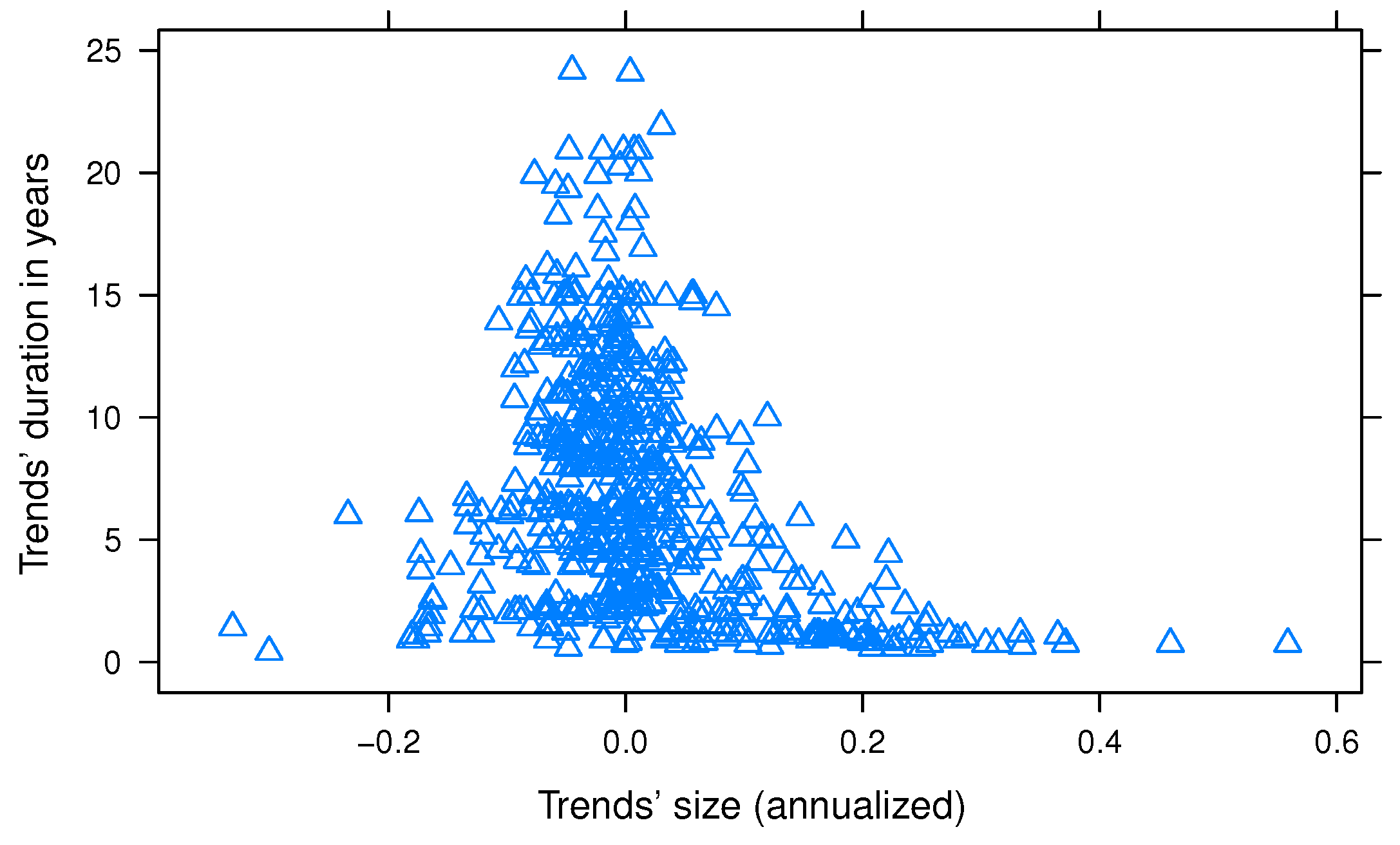
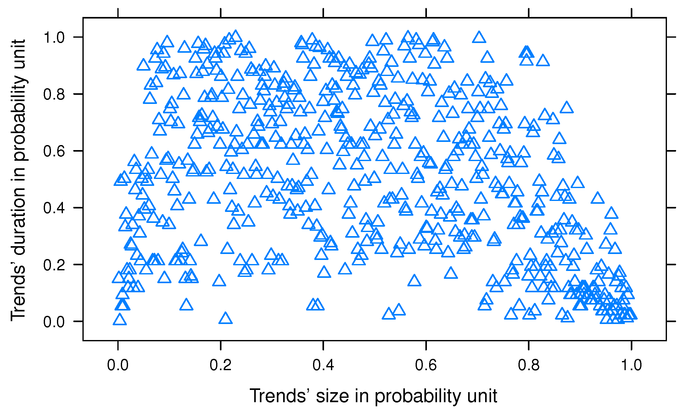
The results suggest that a significant proportion of the plans exhibit non-monotonic trends. We thus deploy the changepoint algorithm explained in Chen and Gupta (2011) to infer these trends from the monthly cash flows. This algorithm is based on hypothesis testing and the bisection method to capture multiple changepoints. The hypothesis tests the statistics of the variance difference between the sub-sectioned time series and the entire series. Interested readers may refer to Hawkins (1977) for additional details. We then manually verify each of these trends to ensure that the algorithm does not over-fit and that there is, at least visually, an observable trend present. After applying the changepoint algorithm, we infer 565 trends for all plans, with their basic statistics described in Table 4. Trend behavior is observed in almost all of the plans we analyze, and we present some of these plans in Appendix B. The figures in the Appendix B clearly show that the discussed trend is dominant across these plans.
Figure 1 and Figure 2 show the relationship and empirical copula of the duration of the trend against the trends’ sizes. A key takeaway from these two Figure 1 and Figure 2 is the hump-shaped relationship between regime trends and their duration. In other words, the empirical data demonstrate that very large trends of inflows or outflows do not persist for extended periods, while mid-size flow trends can persist for longer periods, with some extending for more than 25 years.
We then perform an analysis of the homogeneity of trend data amongst plans. The homogeneity of trend data is a critical factor in making any generic statement about the statistics of trends as a whole. To ensure that the trends are homogeneous among different plans, we analyze the dataset by dividing it into arbitrary subgroups and subjecting them to statistical tests. Our goal is to determine whether the trends were heterogeneous among plans or within groups of plans. To test for homogeneity of variance, we use Levene’s test, Bartlett’s test, and the F-test of equality of variance between two normally distributed sets.5 To avoid bias in subgroup selection, we performed the tests on multiple arbitrary groups. Table 5 shows the recorded lowest p-value we observe in terms of acceptance of the null hypothesis. The test statistics had reasonably high p-values and, as a result, we cannot reject the hypothesis of homogeneity of trends among plans.
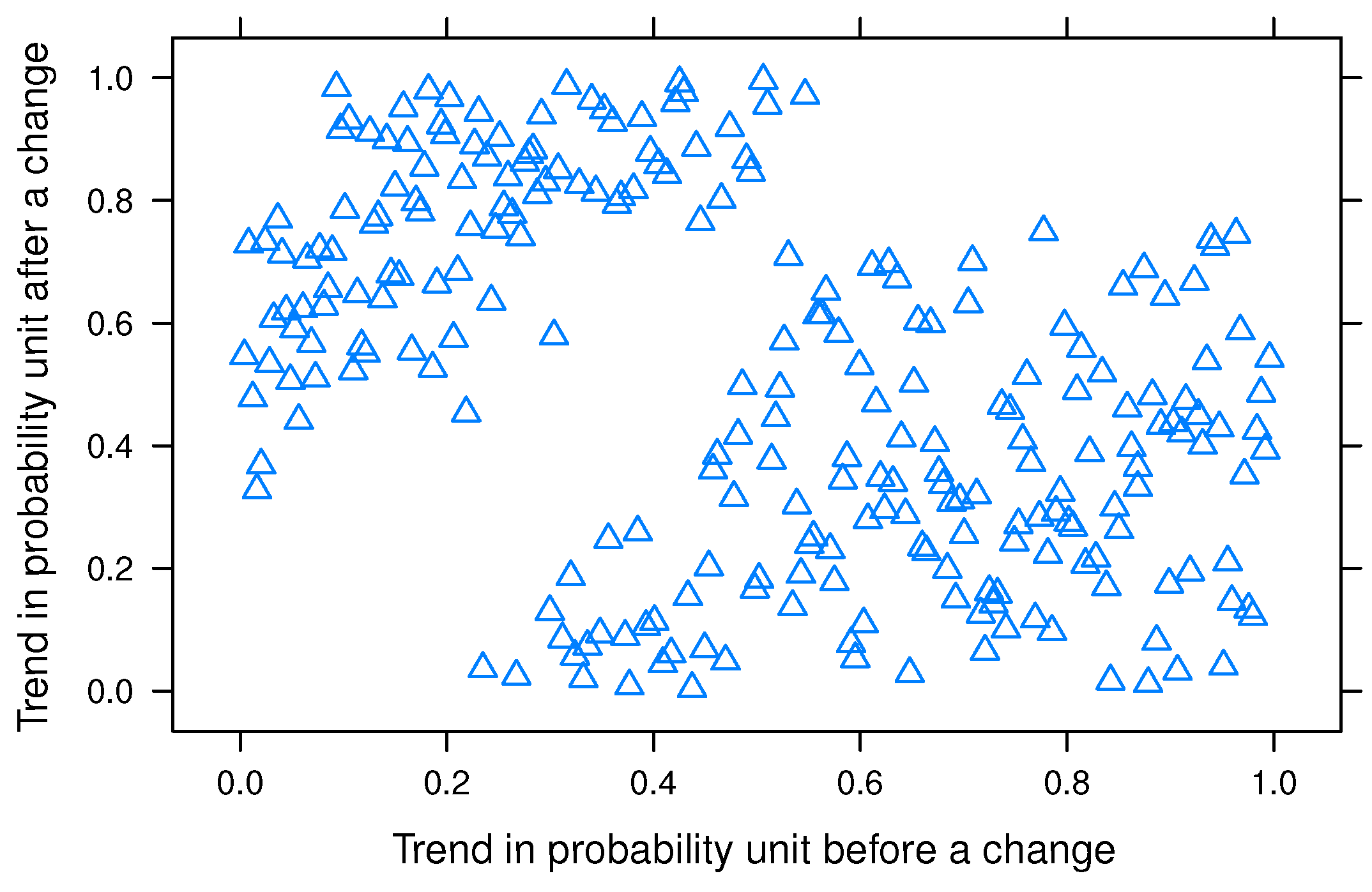
We also seek to understand the relationship between trends before and after a changepoint. To explore this, we generated empirical copulas for trend sizes before and after the changepoint, as depicted in Figure 3. It is important to note that, due to the changepoint algorithm employed, no data points are present around the diagonal in the figure. The statistics are summarized in Table 6. Our analysis led us to conclude no strong relationship exists between trends before and after a changepoint.
Table 6 and Figure 3 show no strong correlation statistics for trends before and after a changepoint. We attribute this lack of relationship to the following economic intuition: the trends are indicative of both idiosyncratic factors affecting the plan sponsor and systemic marketplace conditions, and any changes are often structural and unpredictable. These changes depend on factors such as the financial health of the plan sponsor and management decisions affecting employment, which go beyond quantifiable economic variables; predicting the direction of a trend change caused by an unquantifiable and unpredictable corporate disruption or material change poses significant challenges. This may explain why we do not observe a strong correlation between the size and duration of trends before and after a changepoint. The next section introduces some of the corporate and economic factors contributing to changes in the trends.
4.2. Plan Sponsor’s Ecosystem
Here, we evaluate the relevance of the plan sponsor’s ecosystem hypothesis by focusing on instances of significant changes in trends. Our goal is to determine whether the plan sponsor plays a role in these changes.
To test the hypothesis, we analyze the historical communication for all data points located in the bottom right and top left corners of Figure 3 at the 0.1 centile level (i.e., the two squares from 0.1 to 0.9 centiles and 0.9 to 0.1 centiles). These 30 data points represent the largest change in trends. Our objective is to ascertain whether these changes coincide with a change in the plan sponsors’ ecosystem.
Upon reviewing the corporate communications at the time of the trend change, we find that these changes are associated with macroeconomic, systematic, or corporate-related events. We categorize these events into six common groups as shown in Table 7. Out of these groups, four are related to the plan sponsor ecosystem: “Bankruptcy” (3 out of 30 plans), “Introduction of new investment options” (2 plans), “Post spinoff/merger participant transfer” (6 plans), and “Strong employment growth or reduction” (7 plans). It is worth noting that among these seven plans with strong employment growth or reduction, all of the plans experiencing strong employment growth exhibit a positive trend, while all of the plans with a reduction in employment size demonstrate negative trends. In total, 18 out of the 30 plans with the largest change in trends experience a change in the plan sponsor’s ecosystem. This evidence is sufficient to reject the null hypothesis.
However, we acknowledge that a more robust test would involve comparing the frequency of plan sponsor-related events during the period of the trend change with the frequency of such events for plans/periods without changes in trends. A more persuasive argument would be to verify whether plan sponsor-related events occur less frequently for the other 297-minus-30 plans with weaker changes in trend or during periods without trend changes, compared to the top 30 plans experiencing the largest trend changes. Nonetheless, given the time-consuming nature of examining corporate communications, we are unable to conduct this stronger test.
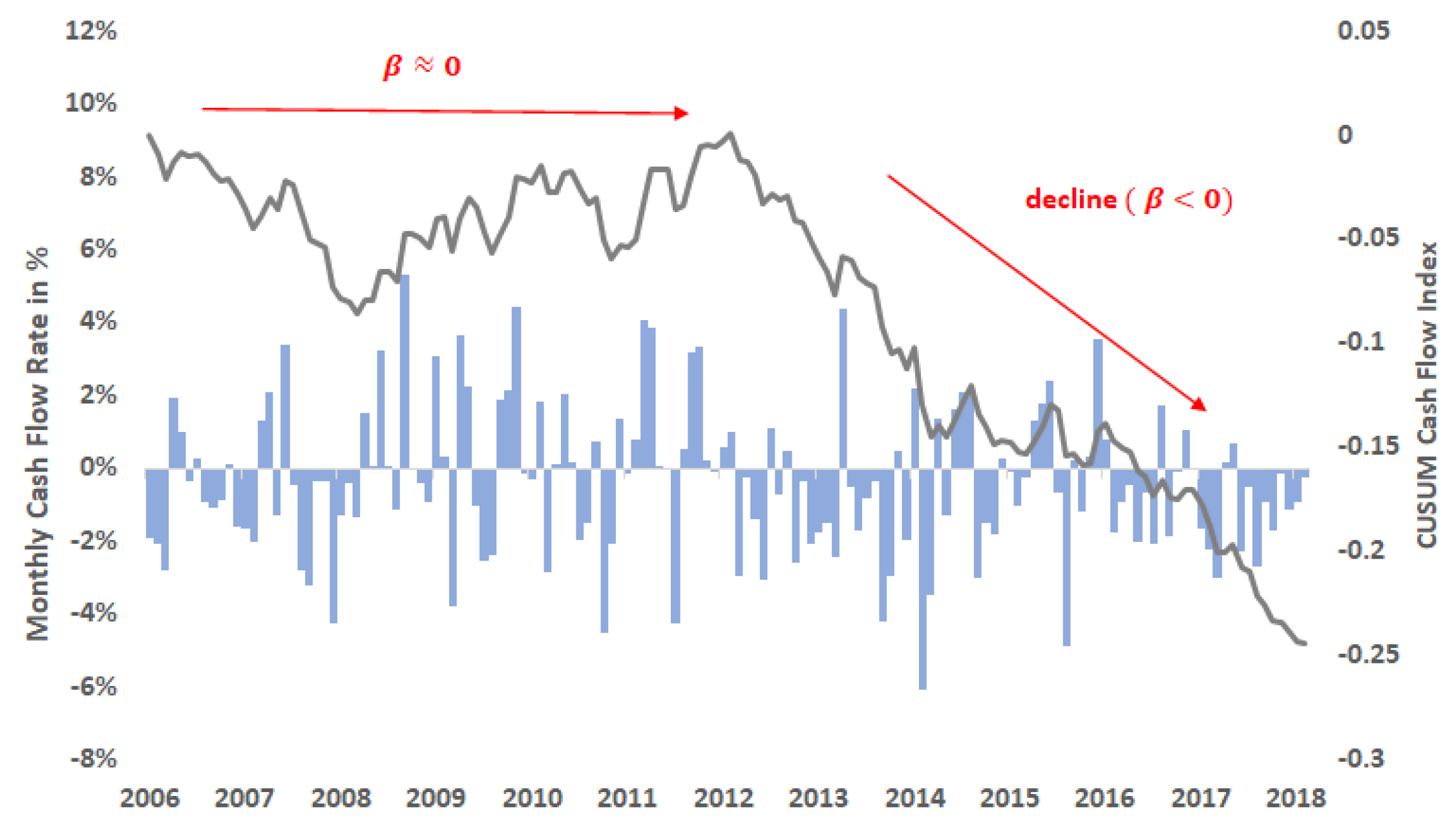
Figure 4 presents a case study of a plan that experienced outflows from their stable value option when the plan sponsor introduced a target date fund to the investment options offered in their 401(k) plan. Our review of the plan sponsor’s communications with participants revealed that they actively promoted the new target date fund as a default option for those who had not chosen a specific investment option. This promotion likely contributed to the increased cash flows into the target date fund.
In summary, our empirical study demonstrates the impact of the employer’s ecosystem on participant cash flows. Factors such as available investment options and changes to these can result in varying behavioral trends. These observations, and our case study, align with the findings of Mitchell and Utkus (2022), who also noted the influence of alternative options, such as target date funds, on 401(k) cash flows. Other studies on the impact of the plan sponsor ecosystem and default options, like Tang et al. (2010), further corroborate our findings.
4.3. Rate Deficit Arbitrage
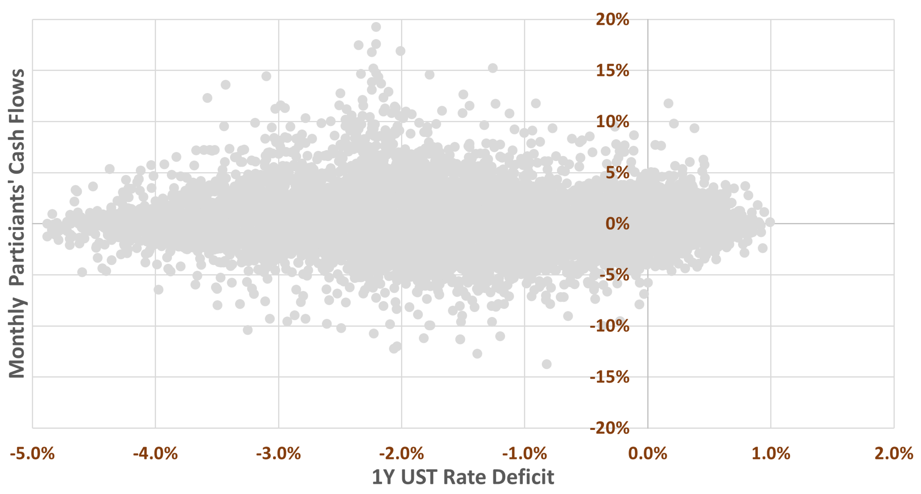
We define the rate deficit as the spread between crediting rates and UST rates (i.e., rate deficit), which serves as an indicator to assess the competitiveness of stable value returns compared to competing funds, such as money market and short-term bond funds. We will use this indicator to test the hypothesis that participants transfer balances from stable value funds to competing funds with higher returns.
To verify this hypothesis, we regress the monthly cash flows for all plans against their respective rate deficit. For this analysis, we use the 1-year UST rate from Federal Reserve Bank of St. Louis (2020). Table 8 summarizes the linear regression statistics for rate deficits and stable value cash flows. The table also assesses the regression results for a 1-year lag. As discussed earlier in Section 2, because the communication of the plan sponsor is based on past performances, there are reasons to consider participants reacting to the rate deficit with a delay. The table shows that the coefficients of determination are low, suggesting that the regressions do not demonstrate a statistically significant linear relationship between the rate differential and stable value cash flows. Figure 5 compares the monthly cash flow data with the 1-year rate deficit, with the range rate deficit observed in the historical data ranging between 1.04% (stable value fund having lower return) and (stable value fund having higher returns).
In conclusion, our analysis did not reveal a strong linear relationship between participant cash flows and the rate deficit, even when a one-year lag was applied. However, it is essential to note that, during the historical period covered by our cash flow data (1997 to 2021), there were no prolonged periods of substantial rate deficits, with the maximum observed rate deficit being only 1.04%. As a result, it can be inferred that participants did not exhibit significant sensitivity to the rate deficit of stable value funds for deficits below 1%.
However, our analysis does not preclude the possibility of a dynamic relationship emerging with larger rate deficits than 1%. Therefore, our findings do not contradict those of Kuo et al. (2003), nor do they refute the rate deficit hypothesis as posited by Sierra Jimenez (2012). It is possible that participant responses might be lagged, although this phenomenon has not been observed within our data period spanning from 1997 to 2021.
The post-2022 period, marked by a shift into a new interest rate regime, provides an intriguing context for further exploration of this hypothesis. Notably, traditional linear regression models may fall short of accurately capturing the dynamics of this altered financial environment. Therefore, it might be advantageous to deploy quantile analysis and regression methods, as suggested by Chen et al. (2022); Yang et al. (2018), or a generalized dynamic factor model similar to Yang (2022), on more recent data from this period.
4.4. Herd Behavior
We define a herding event as a situation in which a substantial number of investors rapidly withdraw funds from a specific investment vehicle within a short period. We consider strong withdrawal rates, defined as any annualized rate above 50% over a 6-month period, as a necessary condition to identify such events. This threshold is based on the concept of herding, which involves the potential for mass withdrawals to rapidly deplete a fund if not addressed. The bottom left of Figure 2 illustrates the location of this threshold in our analysis. By focusing on this specific definition of strong withdrawal rates, we can accurately identify herding events and assess their potential impact on the investment vehicle.
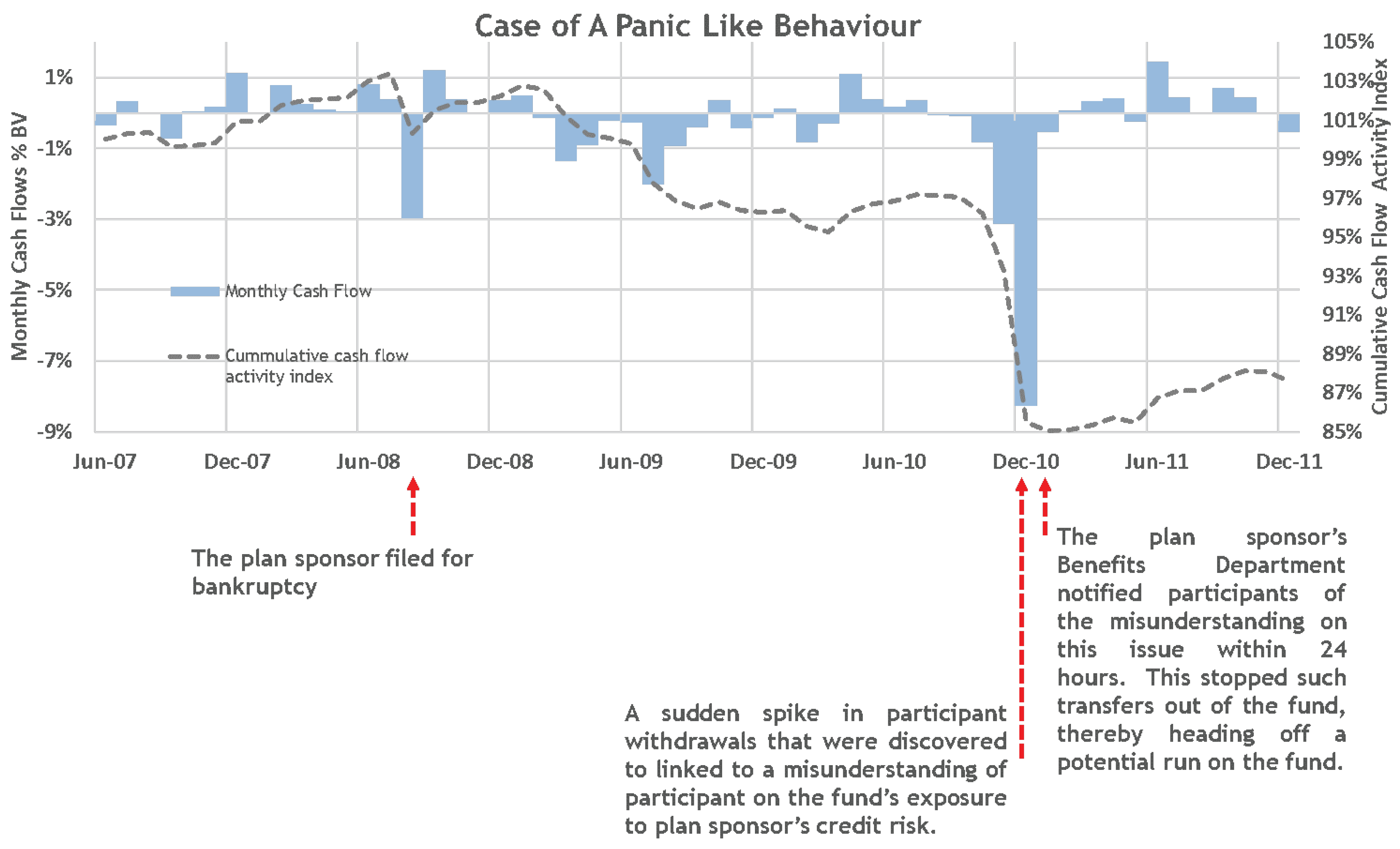
During our analysis of historical data at the plan sponsor level, we discovered one instance where panic-driven behavior in stable value plans led to a significant withdrawal of over 8% of the fund in a single month due to a reputational issue (see Figure 6).
The plan sponsor successfully mitigated the issue by effectively communicating with plan participants within 24 h. The communication reassured participants, addressed their concerns, and ultimately prevented further panic-driven withdrawals. It is worth noting that this behavior raised concerns about the potential amplification of such patterns if not mitigated. Therefore, we considered the possibility of herding behavior, similar to a bank run, leading to the fund’s full or partial depletion.
This case study highlights the importance of efficient plan sponsor communication in mitigating the risks associated with herding behavior, reinforcing the findings of Eberhardt et al. (2021). The significance of the network effect among participants and its potential to trigger herding behavior, as highlighted by Loisel and Milhaud (2011), is also underscored in this case. Moreover, this network effect could potentially be intensified among 401(k) plan participants, as they are all current or former employees of the same company—a scenario akin to bank runs as examined by Vo and Le (2023).
4.5. Flight-to-Safety Behavior
In this subsection, we investigate the flight-to-safety hypothesis, which postulates that, during periods of crisis, investors tend to shift towards more secure investment alternatives to safeguard their assets. Our analysis concentrates on two major crises: the 2008 financial crisis and the COVID-19 pandemic.
We define the financial crisis period as occurring between September 2007 and December 2009, and the COVID-19 pandemic as lasting from January 2020 to June 2021. These definitions are based on our judgment of the market consensus, as opposed to utilizing statistical techniques and financial market indicators, as demonstrated in El-Shagi et al. (2013). We begin our analysis by partitioning the data into three distinct subgroups: the global financial crisis, the COVID-19 pandemic, and other non-crisis periods. We then classify each trend data within these subgroups. A trend data point is regarded as part of a global financial crisis subgroup if its period (start of the trend and ending of the trend) overlaps with our definition of the global financial crisis; the same rule is applied to the COVID-19 pandemic subgroup. However, if a changepoint occurred for a plan during the period of the global financial crisis, then, between the trend data point before or after the changepoint, only the point that had the shortest duration will be part of the global financial crisis subgroup; the same rule is applied to the COVID-19 pandemic subgroup.
Table 9 outlines the data for each subgroup, illustrating the number of trend data points in each category. Some data points may pertain to multiple subgroups, given that the duration of certain trends may coincide with more than one subgroup period. The table enumerates the aggregate number of trend data points for the global financial crisis, the COVID-19 pandemic, and other periods, as well as the number of data points shared between the various subgroups.
Following the data categorization, we aim to test the hypothesis that the distribution of trend data during the global financial crisis and the COVID-19 pandemic is higher than in other normal periods. To do so, we administer a test of stochastic dominance of order 1 among the three subgroups. In this subsection, we present the results of the stochastic dominance tests performed on cash flow samples from three different periods: non-crisis periods, the COVID-19 pandemic, and the global financial crisis (GFC). Specifically, we examined cash flow samples from these three distinct periods using the one-sided Kolmogorov–Smirnov (K-S) test, the Mann–Whitney U test, and the KSPA test Hassani and Silva (2015). While the KSPA test, which is performed on the absolute value of the cash flow trends, does not directly validate the flight-to-safety hypothesis, it can provide valuable insight into whether the size of the trends, regardless of their direction, differs during crisis and non-crisis periods. The results of these tests are presented in Table 10.
Based on a significance level of 0.05, the null hypothesis (H0) is either accepted or rejected. The results of the one-sided Kolmogorov–Smirnov test indicate that the cash flow distributions during non-crisis periods significantly dominate those during the COVID-19 pandemic and the global financial crisis periods. However, there is no significant difference between the cash flow distributions during the COVID-19 pandemic and the global financial crisis.
The Mann–Whitney U test results reveal a significant difference between the cash flow distributions during non-crisis periods and those during the COVID-19 pandemic and the global financial crisis periods. However, no significant difference is found between the cash flow distributions during the COVID-19 pandemic and the global financial crisis.
The KSPA test indicates that the magnitude of cash flow trends during non-crisis periods does not significantly deviate from those during the COVID-19 pandemic or the global financial crisis. It is important to clarify, however, that this test does not directly refute or confirm the flight-to-safety hypothesis. This is because the KSPA test is conducted on the absolute values of the cash flow trends, without considering their directional signs.
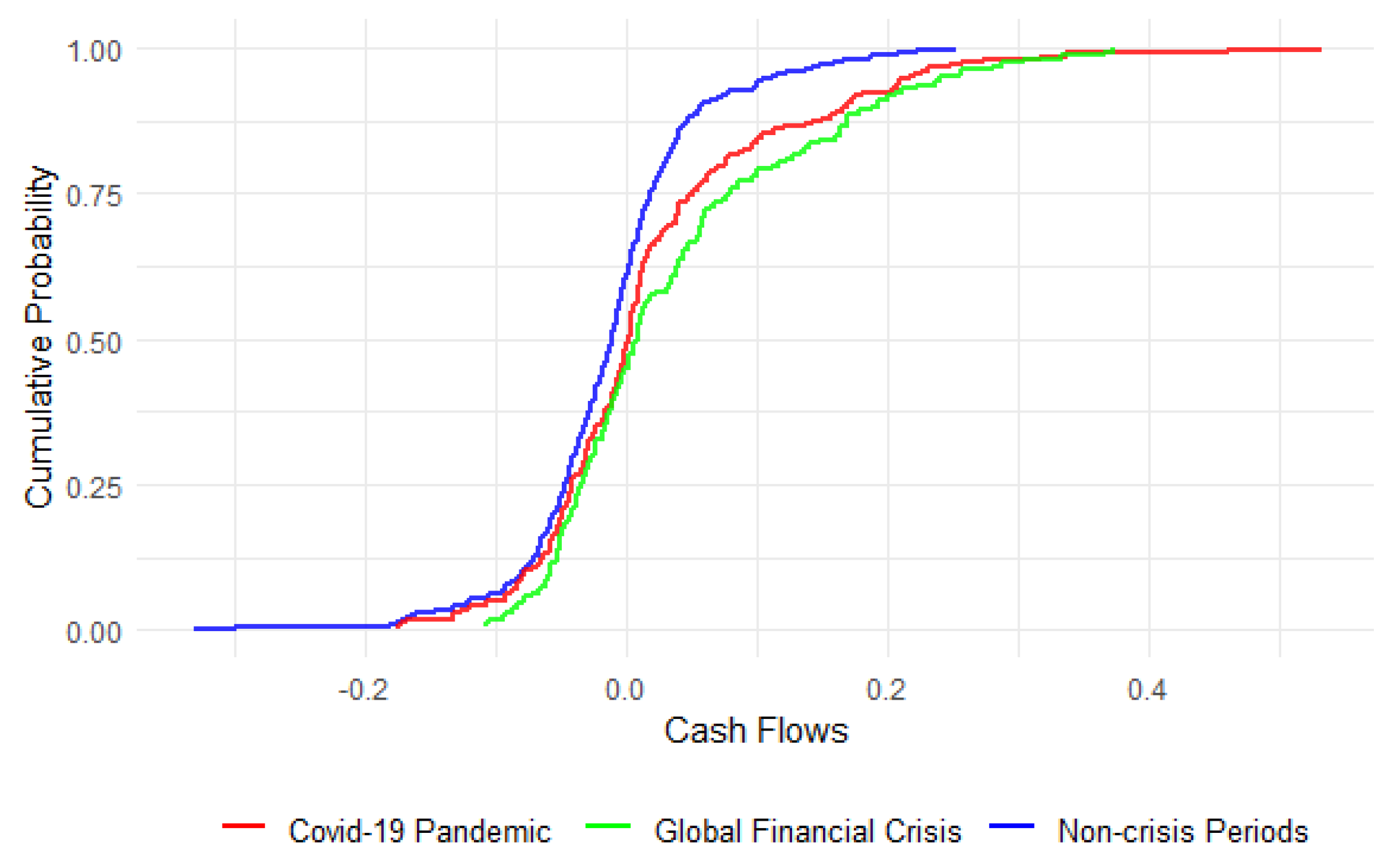
We have also plotted the empirical cumulative distribution function (ECDF) to visually verify the stochastic dominance among the three samples. The plot is shown in Figure 7.
The ECDF plot in Figure 7 provides a visual representation of the cash flow distributions during the non-crisis, COVID-19 pandemic, and global financial crisis periods. The plot confirms the results of the stochastic dominance tests. The cash flow distribution during non-crisis periods (blue line) dominates those during the COVID-19 pandemic (red line) and the global financial crisis (green line), as the blue line is consistently above the red and green lines. The cash flow distributions during the COVID-19 pandemic and the global financial crisis do not show a clear pattern of dominance, which is consistent with the test results.
In essence, our findings suggest that cash flow distributions during non-crisis periods exhibit stochastic dominance over those during crisis periods like the COVID-19 pandemic or the global financial crisis. This lack of significant difference between cash flow distributions during the COVID-19 pandemic and the global financial crisis lends credibility to the “flight-to-safety” hypothesis during these times of uncertainty. Our analysis provides another instance of flight-to-safety behavior besides traditional safe havens like gold and other precious metals, as discussed in Baur and Lucey (2010). Furthermore, our findings align with the research on the flight-to-safety effect during the COVID-19 pandemic as investigated by Ji et al. (2020).
Lastly, to ascertain the robustness of our findings, we conducted sensitivity analyses. The outcomes reveal that minor modifications to the definitions of the crisis periods do not significantly impact the results, further validating our analysis.
4.6. Moneyness Hypothesis
As discussed in Section 2, many works of literature on asset–liability management relate lapsation to the moneyness of the financial product. In this paper, we utilize the market-to-book value (MBV) ratio, which also serves as an asset–liability ratio, as an indicator of the moneyness of a stable value. A lower ratio implies that the assets are more “in the money” in comparison to the liabilities.
To test this, we perform regression testing on the monthly cash flow data. We find no significant relationship between cash flows and MBV ratios, as demonstrated by the low R values in Table 11.
We also observe a stronger relationship between cash flows and MBVs during the global financial crisis, as shown in Table 12. However, the R values remained insignificant, suggesting that, even for these periods, the relationship was not substantial. Note that the relationship between aggregated cash flows and MBV ratios was more pronounced during the global financial crisis due to the “flight-to-safety” effect of stable value investments. Therefore, this relationship is spurious, with the common cause being the “flight-to-safety” effect.
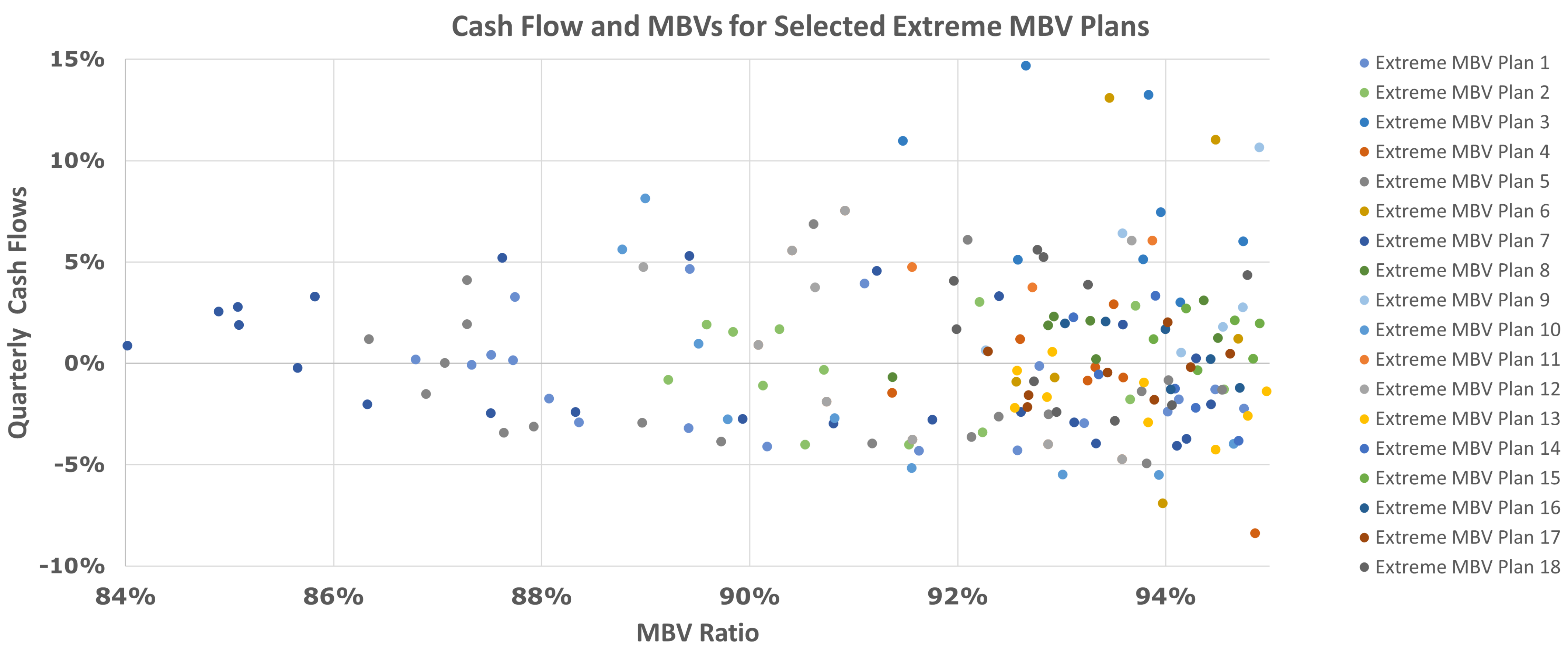
To further support this lack of statistical significance, we study the funds with extremely low MBV ratios, which are potential outliers. We find no statistically significant relationship between MBVs and cash flows in these cases. Figure 8 displays the MBV ratios for 18 plans with extremely low MBV ratios for at least six months (the “Extreme MBV Plans”) and compares them with their quarterly cumulative participant cash flows.
In conclusion, we did not find a strong relationship between participant cash flows and market-to-book values. While the p-values and coefficients of regression were minimal, they were slightly more pronounced during the global financial crisis period. However, we attribute this to the flight-to-safety hypothesis rather than participants being directly sensitive to the market-to-book values.
Our analysis does not align with the findings of Knoller et al. (2016), which discusses the propensity of large policyholders to react to embedded options in variable annuities. We lack individual policyholder data to verify this. However, given that the product we are considering is an insurance product, we tend to believe that the “moneyness” hypothesis may not be as applicable in this context.
Given that the level of market-to-book values (MBVs) observed in our study are all above 85%, a potential alternative approach could have been to employ quantile regression, as described by Yang (2022), or an autoregressive copula model such as Yang and Hamori (2021). However, based on our observations from the graphical analysis above, we argue that even using quantile or non-linear regression methods would not have resulted in significant outcomes in our case. In addition, one unexplored area of improvement in our analysis is to complement with conditional correlation similar to what was carried out in Yang et al. (2018); such an approach could have been used in analyzing the relationship between the MBV and cash flows during different periods like COVID-19 and non-crisis.
5. Discussion and Conclusions
Having conducted a study on participant cash flows in stable value funds using aggregated fund-level data that represents 80% of the individual stable value plans in the market, we found that non-monotonic trends are the dominant factors in stable value cash flow data. We then investigated several hypotheses from the literature that could explain these cash flow trends, including the flight-to-safety effect, rate deficit, herd behavior, mass lapse, and moneyness hypotheses.
On the flight-to-safety effect, our findings indicated that, during crises, participants tend to transfer funds to stable value options as they perceive them as relatively safer.
For the rate deficit hypothesis, we found no evidence of rate arbitrage behaviors in our historical dataset. The absence of direct competitive alternatives within numerous 401(k) plans, coupled with the presence of the equity wash rule, acts as a deterrent for participants to arbitrage their portfolio based on rate deficits. Additionally, plan sponsors typically emphasize past performances in their communication to participants, resulting in delays in responding to rate deficits between investment options, thereby diminishing the significance of this hypothesis. It is also worth noting that we observed limited rate deficit instances from 2000 to 2021 due to stable interest rates. However, our analysis does not provide a conclusion on the impact of high inflationary rates on stable value cash flows, nor the impact of the U.S. interest rates spike post-2022.
Regarding herd behavior and mass lapse, our data shows one case of mass lapse due to a reputational issue. Based on our understanding of the stable value ecosystem, we believe that negative news or rumors about a particular stable value fund or its underlying investments could lead to a loss of confidence among investors, prompting them to withdraw their investments en masse. Therefore, the risk of a reputational mass lapse is plausible but with a low probability of occurrence.
Using the market-to-book value ratio (asset–liability ratio) as an indicator of the moneyness of the stable value products, we verified the moneyness hypothesis. We observe no significant relationship between the market-to-book values and participants’ monthly cash flows. We justify the result obtained by the hypothesis that the moneyness hypothesis is plausible when active trading, such as trading American stock options, is involved. However, the protection offered by stable value funds is an insurance structure rather than a trading one, limiting the relevance of this hypothesis. It is worth noting that a low market-to-book value could potentially be perceived as a weakness and hypothetically lead to reputational issues, increasing the likelihood of herd behavior (even though the case example in Section 4.4 had a market-to-book value close to 100% and the reputational issue was unrelated to its market-to-book).
We conclude that factors such as plan sponsor communication and management decisions, financial health, industry sector, employment policies, growth or layoffs, plan demographics, and default options can impact participant cash flow trends. Therefore, it is crucial to consider these factors when assessing the risk of mass lapses. These factors can influence medium-to-long-term cash flow trends. For instance, our case study in Section 4 reveals participants transferring a portion of their stable value funds to invest in target-date funds when the plan sponsor integrates this option as a default. This finding is consistent with Mitchell and Utkus (2022), who observed a significant proportion of participants transferring funds into target-date funds within the first year of their adoption in 401(k) plans.
Based on our analysis and the conclusions drawn, we suggest that any lapse model built for projecting adverse withdrawal scenarios should consider at least the following risk factors:
- The trend in cash flows is related to the nature of the plan sponsors’ ecosystem, which indirectly influences participants’ behavior.
- A herd behavior component, where the plausibility of this behavior could potentially be influenced by reputational damage6.
- The cash flow risk-mitigating effect of flight-to-safety behavior during a crisis.
Therefore, in terms of future work, an interesting extension of our study could be to integrate our findings within an asset–liability management (ALM) model. This could be particularly useful for evaluating the guarantee risk associated with insurance products. Such a framework could leverage our empirical findings to provide more nuanced risk assessments and strategic insights for both plan sponsors and insurers.
While the statistical evidence did not support a rate deficit effect, there was no historical data available to examine extremely large rate deficits for a long period of time. Given this, a lapse model should also likely consider a rate deficit risk factor that is triggered by deficits significantly higher than 1% and sustained for a period longer than one year.
Also, with inflation on the rise since 2022, it could be insightful to apply a quantile analysis and regression approach to our analysis. This could help us better understand the sensitivity of participant cash flows to rates under the rate deficit hypothesis, following methodologies laid out in studies like Yang et al. (2018) and Chen et al. (2022). However, as of the time of this paper, proprietary data for this period remains unavailable and unprocessed. Given the potential for a time lag in participant responses to rate deficits, this future research opportunity might need more time to come to fruition.
The “flight-to-safety” phenomenon identified in our analysis is a novel insight within the context of stable value funds. A deeper examination of this behavior could offer valuable insights, contributing to our comprehension of participant responses in volatile markets. Specifically, the use of transfer data might shed more light on how participants react under varying market conditions, especially given the direct relevance of the “flight-to-safety” effect to internal transfers within a 401(k) plan between riskier and less risky assets. Regrettably, in this current study, we had access only to net cash flow data (the sum of internal and external transfers within a 401(k) plan), precluding a full examination of transfer data that might more clearly illuminate the “flight-to-safety” effect. Future research that incorporates such data could provide a more nuanced understanding of these patterns.
Author Contributions
Conceptualization and methodology, B.A., J.J., S.L. and Y.S. All authors have read and agreed to the published version of the manuscript.
Funding
S. Loisel acknowledges support from the research chair “Sustainable Actuarial Science and Climate Risks” funded by Milliman Paris.
Data Availability Statement
Restrictions apply to the availability of the data. Data was obtained from Valerian Capital LLC and are available from the authors with the permission of Valerian Capital LLC.
Acknowledgments
The authors extend their sincere appreciation to the five anonymous reviewers, Seware Kangalu, and Alvin Ngugi. Their insightful comments and constructive feedback have contributed to the refinement and improvement of this manuscript.
Conflicts of Interest
The authors declare no conflict of interest.
Appendix A. Basic Data Statistics
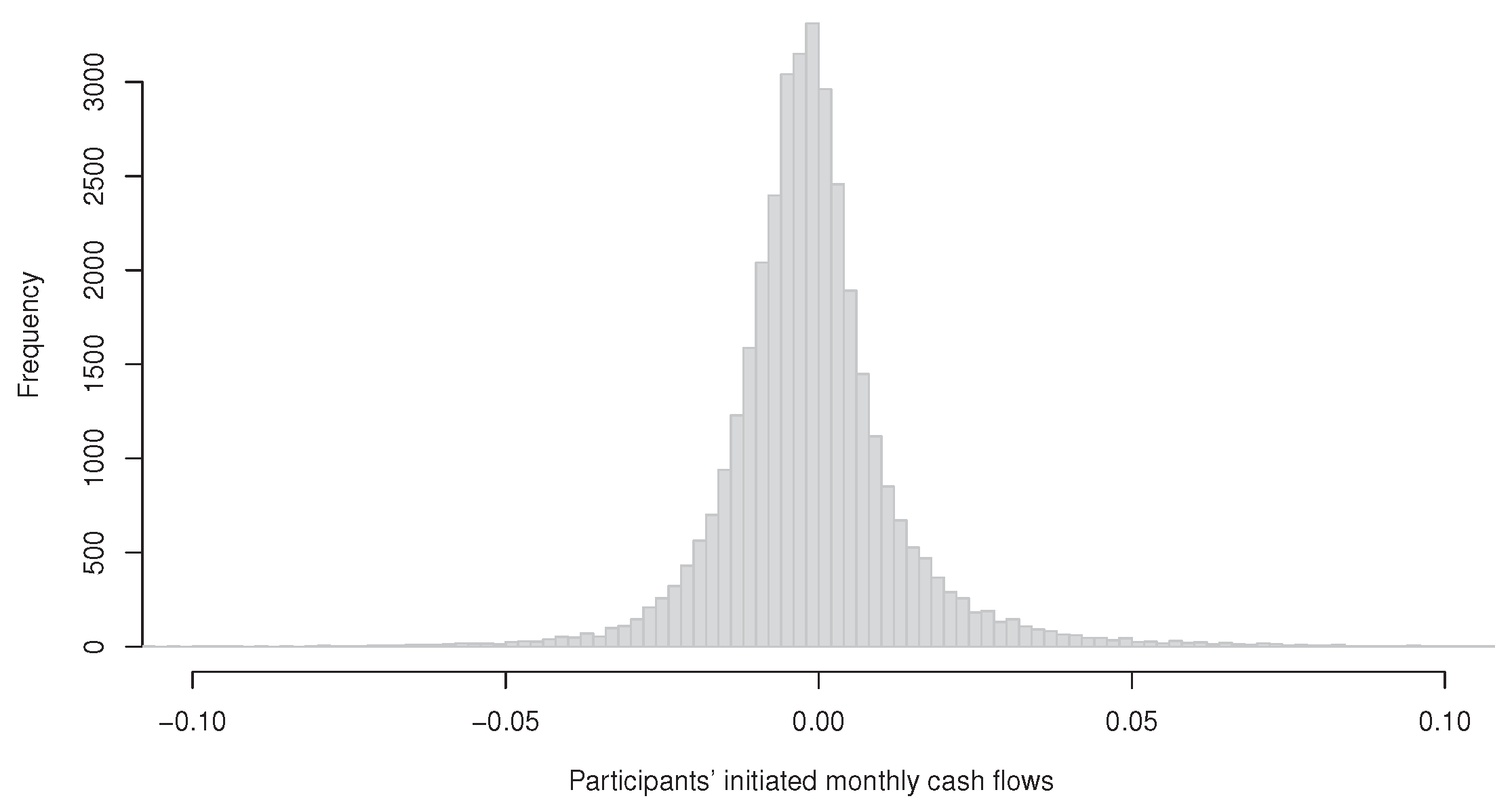
The summary statistics of the participant cash flow data are shown in Table A2. A histogram of the data for the underlying monthly cash flows is shown in Figure A1.

Table A1.
Summary of cash flow data.
| Historical | Book Value | Number of | Number of | |
|---|---|---|---|---|
| Period | Balances (USD) | Plans | Data Points | |
| Jan. 17–Dec. 21 | 132 | billion | 172 | 27,421 |
| Jan. 14–Dec. 21 | 110 | billion | 137 | 24,416 |
| Jan. 8–Dec. 21 | 78 | billion | 38 | 15,710 |
| Nov. 97–Dec. 21 | 222 | billion | 297 | 41,742 |
Table A2.
Statistics of participant-related monthly cash flows.
| Minimum | Maximum | Average | Standard Deviation | Skewness | Kurtosis |
|---|---|---|---|---|---|
Figure A1.
A histogram of monthly cash flows representing data for individual plans. Each observation is expressed as a percentage of the month’s initial book value.
Figure A1.
A histogram of monthly cash flows representing data for individual plans. Each observation is expressed as a percentage of the month’s initial book value.

Appendix B. Example Plans’ Cash Flows with Their Respective Trends


Appendix C. ERISA Communication
The below shows an extract of communication requirements from ERISA’s perspective; see U.S. Department of Labor (2020).
Model Comparative Chart
ABC Corporation 401k Retirement Plan
Investment Options—January 1, 20XX
ABC Corporation 401k Retirement Plan
Investment Options—January 1, 20XX
This document includes important information to help you compare the investment options under your retirement plan. If you want additional information about your investment options, you can go to the specific Internet Web site address shown below or you can contact [insert name of plan administrator or designee] at [insert telephone number and address]. A free paper copy of the information available on the Web site[s] can be obtained by contacting [insert name of plan administrator or designee] at [insert telephone number].
Document Summary
This document has 3 parts. Part I consists of performance information for plan investment options. This part shows you how well the investments have performed in the past. Part II shows you the fees and expenses you will pay if you invest in an option. Part III contains information about the annuity options under your retirement plan.
Part I. Performance Information
Table A3 focuses on the performance of investment options that do not have a fixed or stated rate of return. Table A3 shows how these options have performed over time and allows you to compare them with an appropriate benchmark for the same time periods. Past performance does not guarantee how the investment option will perform in the future. Your investment in these options could lose money. Information about an option’s principal risks is available on the Web site[s].
Table A3.
Variable Return Investments.
| Average Annual Total Return | ||||||||
| as of 12/31/XX | Benchmark | |||||||
| Since | Since | |||||||
| Name/Type of Option | 1 yr. | 5 yr. | 10 yr. | Inception | 1 yr. | 5 yr. | 10 yr. | Inception |
| Equity Funds | ||||||||
| A Index Fund/S&P 500 www. website address | 26.5% | 0.34% | −1.03% | 9.25% | 26.46% | 0.42% | −0.95% | 9.30% |
| S&P 500 | ||||||||
| B Fund/Large Cap www. website address | 27.6% | 0.99% | N/A | 2.26% | 27.80% | 1.02% | N/A | 2.77% |
| US Prime Market 750 Index | ||||||||
| C Fund/Int’l Stock www. website address | 36.73% | 5.26% | 2.29% | 9.37% | 40.40% | 5.40% | 2.40% | 12.09% |
| MSCI EAFE | ||||||||
| D Fund/Mid Cap www. website address | 40.22% | 2.28% | 6.13% | 3.29% | 46.29% | 2.40% | −0.52% | 4.16% |
| Russell Midcap | ||||||||
| Bond Funds | ||||||||
| E Fund/Bond Index www. website address | 6.45% | 4.43% | 6.08% | 7.08% | 5.93% | 4.97% | 6.33% | 7.01% |
| Barclays Cap. Aggr. Bd. | ||||||||
| Other | ||||||||
| F Fund/GICs www. website address | 0.72% | 3.36% | 3.11% | 5.56% | 1.8% | 3.1% | 3.3% | 5.75% |
| 3-month US T-Bill Index | ||||||||
| G Fund/Stable Value www. website address | 4.36% | 4.64% | 5.07% | 3.75% | 1.8% | 3.1% | 3.3% | 4.99% |
| 3-month US T-Bill Index | ||||||||
| Generations 2020/Lifecycle Fund www. website address | 27.94% | N/A | N/A | 2.45% | 26.46% | N/A | N/A | 3.09% |
| S&P 500 | ||||||||
| 23.95% | N/A | N/A | 3.74% | |||||
| Generations 2020 Composite Index * | ||||||||
* Generations 2020 composite index is a combination of a total market index and a US aggregate bond index proportional to the equity/bond allocation in the Generations 2020 Fund.
Table A4 focuses on the performance of investment options that have a fixed or stated rate of return. Table A4 shows the annual rate of return of each such option, the term or length of time that you will earn this rate of return, and other information relevant to performance.
Table A4.
Fixed Return Investments.
| Name/ Type of Option | Return | Term | Other |
|---|---|---|---|
| H 200X/GIC www. website address | 4% | 2 Yr. | The rate of return does not change during the stated term. |
| I LIBOR Plus/Fixed-Type Investment Account www. website address | LIBOR +2% | Quarterly | The rate of return on 12/31/xx was 2.45%. This rate is fixed quarterly, but will never fall below a guaranteed minimum rate of 2%. Current rate of return information is available on the option’s Web site or at 1-800-yyy-zzzz. |
| J Financial Services Co./Fixed Account Investment www. website address | 3.75% | 6 Mos. | The rate of return on 12/31/xx was 3.75%. This rate of return is fixed for six months. Current rate of return information is available on the option’s Web site or at 1-800-yyy-zzzz. |
| 1 | In fact, these connections contribute to non-monotonic trends in participant cash flows, a phenomenon we will delve into in Section 4.1. |
| 2 | In regulatory terminology, the term “hardship” (IRS 2023c) refers to situations where a participant faces financial difficulties. In cases of immediate and substantial financial need, participants can withdraw a portion of their assets without incurring penalties. |
| 3 | ERISA’s requirements form the lowest bar regarding the level of detail and quality of communication expected, and plan administrators may provide more detailed information to participants. |
| 4 | In this paper, we will use the terms plan sponsor, employer, and company interchangeably, even though they may sometimes refer to different legal entities. |
| 5 | However, we should note that F-test statistics assume a normal distribution for both sets, which is not valid for cash flow trends due to their higher tail kurtosis compared to a normal distribution (as indicated in Table 4). |
| 6 | A low market-to-book value could potentially increase the chances of a reputational issue. |
References
- Alfonsi, Aurélien, Adel Cherchali, and Jose Infante. 2019. A full and synthetic model for Asset-Liability Management in life insurance, and analysis of the SCR with the standard formula. European Actuarial Journal 10: 457–98. [Google Scholar] [CrossRef]
- Babbel, David, and Miguel Herce. 2018. An Update on Stable Value Funds Performance through 2017. Journal of Financial Service Professionals 72: 6. [Google Scholar]
- Babbel, David F., and Miguel Herce. 2007. A Closer Look at Stable Value Funds Performance. Working Paper 07-21. Philadelphia: Wharton Financial Institutions Center. [Google Scholar]
- Bacinello, Anna Rita, Pietro Millossovich, Annamaria Olivieri, and Ermanno Pitacco. 2011. Variable annuities: A unifying valuation approach. Insurance: Mathematics and Economics 49: 285–97. [Google Scholar] [CrossRef]
- Barsotti, Flavia, Xavier Milhaud, and Yahia Salhi. 2016. Lapse risk in life insurance: Correlation and contagion effects among policyholders’ behaviors. Insurance: Mathematics and Economics 71: 317–31. [Google Scholar] [CrossRef] [Green Version]
- Barucci, Emilio, Tommaso Colozza, Daniele Marazzina, and Edit Rroji. 2020. The determinants of lapse rates in the italian life insurance market. European Actuarial Journal 10: 149–78. [Google Scholar] [CrossRef] [Green Version]
- Baur, Dirk G., and Brian M. Lucey. 2010. Is gold a hedge or a safe haven? An analysis of stocks, bonds and gold. Financial Review 45: 217–29. [Google Scholar] [CrossRef]
- Butrica, Barbara A., and Karen E. Smith. 2016. 401(k) participant behavior in a volatile economy. Journal of Pension Economics & Finance 15: 1–29. [Google Scholar]
- Chen, Jie, and Arjun K. Gupta. 2011. Parametric Statistical Change Point Analysis: With Applications to Genetics, Medicine, and Finance. Berlin/Heidelberg: Springer Science & Business Media. [Google Scholar]
- Chen, Qitong, Huiming Zhu, Dongwei Yu, and Liya Hau. 2022. How does investor attention matter for crude oil prices and returns? evidence from time-frequency quantile causality analysis. The North American Journal of Economics and Finance 59: 101581. [Google Scholar] [CrossRef]
- Cheng, Chunli, Christian Hilpert, Aidin Miri Lavasani, and Mick Schaefer. 2019. Surrender Contagion in Life Insurance: Modeling and Valuation. European Journal of Operational Research 305: 1465–79. [Google Scholar] [CrossRef]
- Chiang, Thomas C., and Dazhi Zheng. 2010. An empirical analysis of herd behavior in global stock markets. Journal of Banking & Finance 34: 1911–21. [Google Scholar]
- Cumming, Douglas, and Na Dai. 2009. Capital flows and hedge fund regulation. Journal of Empirical Legal Studies 6: 848–73. [Google Scholar] [CrossRef]
- Dar, Atul, and C. Dodds. 1989. Interest rates, the emergency fund hypothesis and saving through endowment policies: Some empirical evidence for the uk. Journal of Risk and Insurance 1989: 415–33. [Google Scholar] [CrossRef]
- De Giovanni, Domenico. 2010. Lapse rate modeling: A rational expectation approach. Scandinavian Actuarial Journal 2010: 56–67. [Google Scholar] [CrossRef]
- Dorn, Daniel, and Gur Huberman. 2005. Talk and action: What individual investors say and what they do. Review of Finance 9: 437–81. [Google Scholar] [CrossRef]
- Eberhardt, Wiebke, Elisabeth Brüggen, Thomas Post, and Chantal Hoet. 2021. Engagement behavior and financial well-being: The effect of message framing in online pension communication. International Journal of Research in Marketing 38: 448–71. [Google Scholar] [CrossRef]
- El-Shagi, Makram, Tobias Knedlik, and Gregor von Schweinitz. 2013. Predicting financial crises: The (statistical) significance of the signals approach. Journal of International Money and Finance 35: 76–103. [Google Scholar] [CrossRef] [Green Version]
- Eling, Martin, and Michael Kochanski. 2013. Research on lapse in life insurance: What has been done and what needs to be done? The Journal of Risk Finance 14: 392–413. [Google Scholar] [CrossRef] [Green Version]
- Federal Reserve Bank of St. Louis. 2020. Moody’s Seasoned Baa Corporate Bond Yield. Available online: https://fred.stlouisfed.org/series/BAA (accessed on 19 July 2023).
- Floryszczak, Anthony, Olivier Le Courtois, and Mohamed Majri. 2016. Inside the solvency 2 black box: Net asset values and solvency capital requirements with a least-squares monte-carlo approach. Insurance: Mathematics and Economics 71: 15–26. [Google Scholar] [CrossRef]
- Hassani, Hossein, and Emmanuel Sirimal Silva. 2015. A kolmogorov-smirnov based test for comparing the predictive accuracy of two sets of forecasts. Econometrics 3: 590–609. [Google Scholar] [CrossRef] [Green Version]
- Hawkins, Douglas M. 1977. Testing a sequence of observations for a shift in location. Journal of the American Statistical Association 72: 180–86. [Google Scholar] [CrossRef]
- Hirshleifer, David, and Siew Hong Teoh. 2003. Herd behaviour and cascading in capital markets: A review and synthesis. European Financial Management 9: 25–66. [Google Scholar] [CrossRef]
- IRS. 2023a. 401k Resource Guide Plan Participants General Distribution Rules. Available online: https://www.irs.gov/retirement-plans/plan-participant-employee/401k-resource-guide-plan-participants-general-distribution-rules (accessed on 19 July 2023).
- IRS. 2023b. Retirement Plan Distributions: Exceptions to 10% Additional Tax. Available online: https://www.irs.gov/pub/irs-pdf/p5036.pdf (accessed on 19 July 2023).
- IRS. 2023c. Retirement Topics—Hardship Distributions. Available online: https://www.irs.gov/retirement-plans/plan-participant-employee/retirement-topics-hardship-distributions (accessed on 19 July 2023).
- Ji, Qiang, Dayong Zhang, and Yuqian Zhao. 2020. Searching for safe-haven assets during the COVID-19 pandemic. International Review of Financial Analysis 71: 101526. [Google Scholar] [CrossRef]
- Kalantonis, Petros, Christos Kallandranis, and Marios Sotiropoulos. 2021. Leverage and firm performance: New evidence on the role of economic sentiment using accounting information. Journal of Capital Markets Studies 5: 96–107. [Google Scholar] [CrossRef]
- Kim, Changki. 2005. Modeling surrender and lapse rates with economic variables. North American Actuarial Journal 9: 56–70. [Google Scholar] [CrossRef]
- Knoller, Christian, Gunther Kraut, and Pascal Schoenmaekers. 2016. On the propensity to surrender a variable annuity contract: An empirical analysis of dynamic policyholder behavior. Journal of Risk and Insurance 83: 979–1006. [Google Scholar] [CrossRef]
- Kuo, Weiyu, Chenghsien Tsai, and Wei-Kuang Chen. 2003. An empirical study on the lapse rate: The cointegration approach. Journal of Risk and Insurance 70: 489–508. [Google Scholar] [CrossRef]
- Kwun, David, Cyrus Mohebbi, Andrew Line, and Yong-Tai Tsai. 2009. A risk analysis of stable value protection for bank-owned life insurance. International Journal of Applied Decision Sciences 2: 406–21. [Google Scholar] [CrossRef]
- Kwun, David, Cyrus Mohebbi, Marc Braunstein, and Andrew Line. 2010. A risk analysis of 401k stable value funds. International Journal of Applied Decision Sciences 3: 151–67. [Google Scholar] [CrossRef]
- Loisel, Stéphane, and Xavier Milhaud. 2011. From deterministic to stochastic surrender risk models: Impact of correlation crises on economic capital. European Journal of Operational Research 214: 348–57. [Google Scholar] [CrossRef] [Green Version]
- Lyubchich, Vyacheslav, Yulia R. Gel, and Abdel El-Shaarawi. 2013. On detecting non-monotonic trends in environmental time series: A fusion of local regression and bootstrap. Environmetrics 24: 209–26. [Google Scholar] [CrossRef]
- Madrian, Brigitte C., and Dennis F. Shea. 2001. The power of suggestion: Inertia in 401(k) participation and savings behavior. The Quarterly Journal of Economics 116: 1149–87. [Google Scholar] [CrossRef] [Green Version]
- Mahdavi-Damghani, Babak. 2012. Utope-ia. Wilmott 2012: 28–37. [Google Scholar]
- Mitchell, Olivia S., and Stephen P. Utkus. 2022. Target-date funds and portfolio choice in 401 (k) plans. Journal of Pension Economics & Finance 21: 519–36. [Google Scholar]
- Mitchell, Olivia S., Gary R. Mottola, Stephen P. Utkus, and Takeshi Yamaguchi. 2006. The Inattentive Participant: Portfolio Trading Behavior in 401(K) Plans. Working Paper WP 2006-115. London: Michigan Retirement Research Center. [Google Scholar]
- Outreville, J. Francois. 1990. Whole-life insurance lapse rates and the emergency fund hypothesis. Insurance: Mathematics and Economics 9: 249–55. [Google Scholar] [CrossRef]
- Phillips, Joseph M., Jr., Barry B. Schweig, and James P. Scott. 1985. Explaining whole life insurance lapse rates. The Journal of Insurance Issues and Practices 1985: 32–40. [Google Scholar]
- Shin, Hyun Song. 2009. Reflections on northern rock: The bank run that heralded the global financial crisis. Journal of Economic Perspectives 23: 101–19. [Google Scholar] [CrossRef] [Green Version]
- Sierra Jimenez, Jesus A. 2012. Consumer Interest Rates and Retail Mutual Fund Flows. Available online: https://www.bankofcanada.ca/2012/12/working-paper-2012-39/ (accessed on 19 July 2023).
- SVIA. 2020a. Stable Value at a Glance. Available online: https://www.stablevalue.org/knowledge/stable-value-at-a-glance (accessed on 19 July 2023).
- SVIA. 2020b. Stable Value Quarterly Characteristic Survey. California: SVIA, December. [Google Scholar]
- Tang, Ning, Olivia S. Mitchell, Gary R. Mottola, and Stephen P. Utkus. 2010. The efficiency of sponsor and participant portfolio choices in 401 (k) plans. Journal of Public Economics 94: 1073–85. [Google Scholar] [CrossRef] [Green Version]
- Tobe, Christopher B. 2004. The Consultants Guide to Stable Value. Journal of Investment Consulting 7: 1. [Google Scholar]
- Tsai, Chenghsien, Weiyu Kuo, and Wei-Kuang Chen. 2002. Early surrender and the distribution of policy reserves. Insurance: Mathematics and Economics 31: 429–45. [Google Scholar] [CrossRef]
- U.S. Department of Labor. 2020. Model Comparative Chart—ABC Corporation 401k Retirement Plan. Available online: https://www.dol.gov/sites/dolgov/files/ebsa/about-ebsa/our-activities/resource-center/publications/providing-information-in-participant-directed-plans-model-chart.pdf (accessed on 19 July 2023).
- Vo, Lai Van, and Huong T. T. Le. 2023. From hero to zero-the case of silicon valley bank. Electronic Journal 2023: 1–22. [Google Scholar]
- Wang, Lan, Michael G. Akritas, and Ingrid Van Keilegom. 2008. An anova-type nonparametric diagnostic test for heteroscedastic regression models. Journal of Nonparametric Statistics 20: 365–82. [Google Scholar] [CrossRef]
- Xiong, James X., and Thomas M. Idzorek. 2012. Estimating credit risk and illiquidity risk in guaranteed investment Products. Journal of Financial Planning 25: 38–47. [Google Scholar]
- Yang, Lu. 2022. Idiosyncratic information spillover and connectedness network between the electricity and carbon markets in europe. Journal of Commodity Markets 25: 100185. [Google Scholar] [CrossRef]
- Yang, Lu, and Shigeyuki Hamori. 2021. The role of the carbon market in relation to the cryptocurrency market: Only diversification or more? International Review of Financial Analysis 77: 101864. [Google Scholar] [CrossRef]
- Yang, Lu, Shuairu Tian, Wei Yang, Mingli Xu, and Shigeyuki Hamori. 2018. Dependence structures between chinese stock markets and the international financial market: Evidence from a wavelet-based quantile regression approach. The North American Journal of Economics and Finance 45: 116–37. [Google Scholar] [CrossRef]
Figure 1.
Empirical data for trends and their respective duration.

Figure 2.
Empirical copulas for trends and their respective duration.

Figure 3.
Empirical copulas for trends before and after a changepoint.

Figure 4.
Change in trends in withdrawal from a stable value fund due to the introduction of target-date funds within the plan.
Figure 4.
Change in trends in withdrawal from a stable value fund due to the introduction of target-date funds within the plan.

Figure 5.
Historical data of the relationship between cash flow rate as a function of the crediting rate deficit to the 1-year UST rates.
Figure 5.
Historical data of the relationship between cash flow rate as a function of the crediting rate deficit to the 1-year UST rates.

Figure 6.
Case of panic-like withdrawal behavior by plan participants.

Figure 7.
ECDF of cash flows during non-crisis, COVID-19 pandemic, and global financial crisis periods.
Figure 7.
ECDF of cash flows during non-crisis, COVID-19 pandemic, and global financial crisis periods.

Figure 8.
Quarterly cash flows for the lowest MBV ratio observed.

Table 1.
The 401(k) withdrawal penalty exceptions.
| Early Withdrawal | |
|---|---|
| Age | After participant/IRA owner reaches age 59½ |
| Death | After the death of the participant/IRA owner |
| Disability | Total and permanent disability of the participant |
| Domestic relations | To an alternate payee under a Qualified Domestic Relations Order |
| Medical health | Insurance premiums paid while unemployed, amount of non-reimbursed medical expenses up to a limit |
| Rollover | In-plan Roth rollovers or eligible distributions contributed to another retirement plan or IRA |
| Hardship | |
| Medical | Medical care expenses for the employee, the employee’s spouse, dependents, or beneficiary |
| Housing | Costs directly related to the purchase of an employee’s principal residence (excluding mortgage payments) Payments necessary to prevent the eviction of the employee from the employee’s principal residence or foreclosure on the mortgage on that residence Certain expenses to repair damage to the employee’s principal residence |
| Education | Tuition, related educational fees, and room and board expenses for the next 12 months of post-secondary education for the employee or the employee’s spouse, children, dependents, or beneficiary |
| Death | Funeral expenses for the employee, the employee’s spouse, children, dependents, or beneficiary |
| Loans | |
| Loans | The maximum amount a participant may borrow from the plan is 50% of the account balance or USD 50,000, whichever is less |
Table 2.
Results of the Ljung–Box and Durbin–Watson tests for participant cash flows in stable value funds.
Table 2.
Results of the Ljung–Box and Durbin–Watson tests for participant cash flows in stable value funds.
| Test | Number of Plans Not Rejected | Number of Plans Rejected |
|---|---|---|
| Durbin–Watson | 134 | 184 |
| Ljung–Box (Lag 12) | 185 | 133 |
| Ljung–Box (Lag 1) | 162 | 156 |
Table 3.
Results of the WAVK test for non-monotonic trends.
| Test | Number of Plans Not Rejected | Number of Plans Rejected |
|---|---|---|
| WAVK | 154 | 126 |
Table 4.
Statistics for participant trends.
| Standard | ||||||
|---|---|---|---|---|---|---|
| Minimum | Maximum | Average | Deviation | Skewness | Kurtosis | |
| Trends’ size * | ||||||
| Trends’ duration | 6 months | 24.5 years | 7.5 years | 5.3 years |
* The measures for the trend sizes are annualized percentages.
Table 5.
Test of homogeneity for participants’ cash flow trends.
| Test | Test Stat. | p-Value |
|---|---|---|
| F-test | 1.3243 | 0.06 |
| Bartlett’s test | 3.824 | 0.06 |
| Levene test | 1.7823 | 0.1825 |
| Chi-square test | 3.7830 | 0.2394 |
Table 6.
Statistics for correlation of trends before and after a changepoint.
| Spearman Corr | Kendall Tau | |
|---|---|---|
| Current trend size and next trend size | −0.083 | −0.029 |
| Current duration and next trend size | 0.048 | 0.034 |
Table 7.
Plans that experienced the largest change in trend with explanations found in corporate communications.
Table 7.
Plans that experienced the largest change in trend with explanations found in corporate communications.
| Event Occurring during the Period of a Drastic Change in Trend | Number of Plans | Trend Sign |
|---|---|---|
| Bankruptcy | 3 | Negative |
| Employment growth or reduction | 7 | Respectively + and − |
| Flight to safety during crisis | 11 | Positive |
| Introduction of new investment options with being the default options | 2 | Negative |
| Post spinoff/merger participant voluntary transfer to/from new investment scheme | 6 | Spinoffs: +, Mergers + or − |
| Reputational issues leading mass withdrawal | 1 | Negative |
Table 8.
Results of cash flows against 1-year UST rate deficit, with a one-year lag.
| Coefficient | Number of | ||||
|---|---|---|---|---|---|
| Lag | Correlation | R | of Regression | p-Value | Data Points |
| 0 y | 1.8% | 0.03% | 2.9% | 0.04% | 36,259 |
| 1 y | 2.7% | 0.06% | 3.5% | 0.06% | 36,259 |
Table 9.
Subgroups of segregated data.
| Subgroup | Number of (Trend) Data Points |
|---|---|
| Group 1: global financial crisis | 158 |
| Group 2: COVID-19 pandemic | 207 |
| Group 3: non-crisis periods | 489 |
| Common in Group 1 and 3 | 0 |
| Common in Group 2 and 3 | 178 |
| Common in Group 1, 2, and 3 | 0 |
Table 10.
Stochastic dominance test results.
| Test | Comparison | Test Statistic | p-Value | Decision | |
|---|---|---|---|---|---|
| K-S (Greater) | Non-crisis vs. COVID-19 | 5.79 | Reject | ||
| K-S (Greater) | Non-crisis vs. GFC | 1.11 | Reject | ||
| K-S (Greater) | COVID-19 vs. GFC | 9.83 | Not Reject | ||
| Mann–Whitney U | Non-crisis vs. COVID-19 | 2.34 | Reject | ||
| Mann–Whitney U | Non-crisis vs. GFC | 7.44 | Reject | ||
| Mann–Whitney U | COVID-19 vs. GFC | 1.46 | Not Reject | ||
| KSPA | Non-crisis vs. COVID-19 | 9.96 | Not Reject | ||
| KSPA | Non-crisis vs. GFC | 9.83 | Not Reject | ||
| KSPA | COVID-19 vs. GFC | 4.31 | Reject |
Table 11.
Results of market-to-book value ratio regression against fund-level cashflows.
| Coefficient of | Number of | ||
|---|---|---|---|
| Correlation | Determination | p-Value | Observations |
| 4.12 | 1.46 | 35,049 |
Table 12.
MBV ratios regressed against cash flows during the global financial crisis and the COVID-19 pandemic.
Table 12.
MBV ratios regressed against cash flows during the global financial crisis and the COVID-19 pandemic.
| Coefficient of | Number of | |||
|---|---|---|---|---|
| Period | Correlation | Determination | p-Value | Observations |
| Global Financial Crisis | −1.78 | 3.18 | 0.00 | 4893 |
| COVID-19 Pandemic | −3.40 | 1.2 | 2.97 | 4108 |
Disclaimer/Publisher’s Note: The statements, opinions and data contained in all publications are solely those of the individual author(s) and contributor(s) and not of MDPI and/or the editor(s). MDPI and/or the editor(s) disclaim responsibility for any injury to people or property resulting from any ideas, methods, instructions or products referred to in the content. |
© 2023 by the authors. Licensee MDPI, Basel, Switzerland. This article is an open access article distributed under the terms and conditions of the Creative Commons Attribution (CC BY) license (https://creativecommons.org/licenses/by/4.0/).
Share and Cite
MDPI and ACS Style
Alimoradian, B.; Jakubiak, J.; Loisel, S.; Salhi, Y. Understanding Key Drivers of Participant Cash Flows for Individually Managed Stable Value Funds. Risks 2023, 11, 148. https://doi.org/10.3390/risks11080148
AMA Style
Alimoradian B, Jakubiak J, Loisel S, Salhi Y. Understanding Key Drivers of Participant Cash Flows for Individually Managed Stable Value Funds. Risks. 2023; 11(8):148. https://doi.org/10.3390/risks11080148
Chicago/Turabian StyleAlimoradian, Behzad, Jeffrey Jakubiak, Stephane Loisel, and Yahia Salhi. 2023. "Understanding Key Drivers of Participant Cash Flows for Individually Managed Stable Value Funds" Risks 11, no. 8: 148. https://doi.org/10.3390/risks11080148
Note that from the first issue of 2016, this journal uses article numbers instead of page numbers. See further details here.