Quantized Approach to Damped Transversal Mechanical Waves

Abstract

In information transfer, the dissipation of a signal is of crucial importance. The feasibility of reconstructing the distorted signal depends on the related permanent loss. Therefore, understanding the quantized dissipative transversal mechanical waves might result in deep insights. In particular, it may be valid on the nanoscale in the case of signal distortion, loss, or even restoration. Based on the description of the damped quantum oscillator, we generalize the canonical quantization procedure for the case of the transversal waves. Then, we deduce the related damped wave equation and the state function. We point out the two possible solutions of the propagating-damping wave equation. One involves the well-known Gaussian spreading solution superposed with the damping oscillation, in which the loss of information is complete. The other is the Airy function solution, which is non-spreading–propagating, so the information loss is only due to oscillation damping. However, the structure of the wave shape remains unchanged for the latter. Consequently, this fact may allow signal reconstruction, resulting in the capability of restoring the lost information.

1. Introduction

Quantum-based signal propagation is the focus of information transfer today. The correct and rigorous description of signal loss due to dissipation or the possible restoration after the loss is a challenge in the examination. It seems obvious that if we knew the correct formulation of the mechanism of loss, the reconstruction of the signal may be within reach. In the present work, we investigate the quantum mechanical problem of damped transversal wave propagation. This mechanical process, interacting with other physical phenomena, like thermal energy [1], electric charge transfers [2,3], spin waves, spin relaxation processes [4,5,6,7], spin wave computing [8], operation in quantum computers [9], or quantum computation on novel solid-state qubit platforms [10,11,12], may cause unexpected deviance in their realization or in signal reconstruction. Further experimental and theoretical motivations to incorporate dissipation into quantum theories can be found in Haken’s [13] and Haake’s [14] early works.

The desire to develop a consequent quantization procedure for the damped oscillator dates as early as quantum mechanics itself. There are many different ideas and methods for resolving this dissipative physical problem. The methods are based on non-conserving subsystems (Caldirola, Kanai) [15,16], explicit time-dependent formulations (Dekker, Dittrich et al) [17,18] that cause incompatibility with the uncertainty principle (Weiss) [19], decoupled harmonic oscillators in a reservoir (Leggett, and Caldeira et al) [20,21,22], or on the further development of Caldirola’s, and Kanai’s procedure (Choi) [23]. A recent study by Bagarello et al. [24] discusses why there are certain doubts about quantizing Bateman’s damped oscillator description [25]. A second quantized solution is presented by Risken [26]. In this method, there is no frequency shift, and only the amplitude is damped. An even more recent paper, by Serhan et al.[27,28], developed a Wentzel–Kramers–Brillouin (WKB) approximation-based quantization procedure to study the damped quantum oscillator. The latter is an explicit time-dependent Lagrangian method resulting in an exponentially decreasing time-dependent wave function, but it is a standing solution in space. For quantum dissipative systems, El-Nabulsi [29] suggested the introduction of dynamical friction in the theory. However, the velocity-dependent term does not appear in the equation of motion, which generates exponential time relaxation.

The Lagrangian least action principle, including dissipative processes, is at the center of coupled quantum or classical irreversible field theoretical processes. Considering all the above mentioned, the following necessary step towards the mathematical formulation of quantum dissipative processes is the Lagrangian construction of the dissipative harmonic oscillator [30]. The mathematical structure provides a consistent and non-contradictory system for the canonical quantities, the Hamiltonian function, and through them, the evolution of the physical quantities over time. The developed Lagrange–Hamilton framework allows for the introduction of the canonical quantization of the damped oscillator. The presented procedure is somewhat different from the usual. Nevertheless, the state equation and its related solution for the damped oscillator are completely identical to our physical picture [31]. If the damping is identified with a shearing effect, we can develop the physical idea that the oscillation is part of a transversal mechanical wave. Following this line of thought, the quantization procedure can be transferred to the canonical quantization of this mechanical wave. As a result, the transversal wave is composed of local vertical damped oscillation and free propagation along the horizontal direction. The internal shearing causes the damping effect, and the generated longitudinal motion is considered dissipation-free. The related quantization procedure provides the quantized transversal mechanical wave equation and the wave solutions. We can distinguish two kinds of solutions. One of these is the well-known Gaussian spreading solution [32]. The other one is the so-called Airy beam solution [33], which relates to a rather strange propagating mode. However, there is experimental evidence for this kind of propagation in other fields of physics [34,35,36,37,38,39,40,41]. If this solution existed in the case of quantized mechanical waves, it could be of great importance from the point of view of the reconstruction of distorted signals.

The mathematical model we devised contains fourth-order derivatives. It is known that stability problems [42] and unlimitedly growing solutions to such equations can arise in the solutions to such equations. We will make the necessary comments in the appropriate places. Now, we only mention that there are equations with a similar structure, where additional factors ensure the real dynamics, e.g., the Dysthe equation [43,44,45], which is a fourth-order modified nonlinear Schrödinger equation for describing water waves. Likewise, fourth-order equations are relevant and applicable to other areas of physics [46,47].

The article is structured as follows: In the second part (Section 2), we summarize the canonical description of the dissipative harmonic oscillator to the necessary extent. We give a brief overview of the damped oscillator quantization method in the third part (Section 3). Based on the results of the quantized damped oscillator, we extend the quantization procedure for to case of the transversal mechanical wave. In the fourth part (Section 4), we establish the related commutation rules; we calculate the Hamiltonian; then, we formulate the quantum state equation of the damped transversal mechanical wave. We discuss the solutions to the state equation in the fifth part (Section 5). We point out the possible Gaussian spreading and the non-spreading Airy beam solutions. In the last part (Section 6), we summarize and conclude the obtained results, and we present a future outlook.

2. The Canonical Description of a Damped Harmonic Oscillator

As an initial step, we need to split the transversal mechanical wave motion into damped oscillation and free translation. This allows us to deal with the oscillation motion and the wave propagation separately. The damping of the oscillator is a physical consequence of the internal friction; i.e., in the transversal propagation, a shear interaction appears, similarly to viscosity. We assume that this shearing effect is proportional to the oscillation velocity, and its y-directional motion is perpendicular to the x-direction of traveling wave propagation. The shearing force makes the oscillator’s motion dissipative. We perform the calculations in parts. First, we examine the Lagrangian description of the motion of the damped harmonic oscillator.

$$\ddot{y}+2\lambda \dot{y}+{\omega }^{2}y=0,$$

(1)

where $\lambda$ [1/s] is a specific damping factor and $\omega$ [1/s] is the angular frequency of the free oscillator. In general, the Lagrangian formulation requires the introduction of generator potentials in the case of non-selfadjoint operators [48,49], like the first-order time derivative, here. This difficulty also appears in electrodynamics [50]. The Lagrangian frame can only be applied through the introduction of the vector potential, which generates the measurable fields. For this reason, we need to express the measurable quantity, y, by the potential, q [m s²], as the definition equation shows [30]:

$$y=\ddot{q}-2\lambda \dot{q}+{\omega }^{2}q.$$

(2)

Then, a potential-based Lagrangian is constructed, which serves as the equation of motion.

$$L=\frac{1}{2}{\left(\ddot{q}-2\lambda \dot{q}+{\omega }^{2}q\right)}^2.$$

(3)

In the case of the second-order derivatives, there are two generalized coordinates and two canonical momenta [31]. Applying the related variational calculus procedure for higher-order derivatives—up to the second order here—in the Lagrangian [51], we must define two generalized coordinates, and there are two coupled generalized momenta. (In general, the order of the derivatives equals the number of generalized coordinates.) We consider these coordinates as independent variables; by definition,

$$q_1:=q,$$

(4)

and

$$q_2:=\dot{q}.$$

(5)

In this particular case, the conjugated momentum, $p_1$ [m/s] to $q_1$ [m s²], is

$$p_1:=\frac{\partial L}{\partial \dot{q}}-\frac{\mathrm{d}}{\mathrm{d}t}\frac{\partial L}{\partial \ddot{q}}=4{\lambda }^2\dot{q}-\stackrel{⃛}{q}-{\omega }^2\dot{q}-2\lambda {\omega }^{2}q.$$

(6)

The second momentum, $p_2$ [m] to $q_2$ [m s], is

$$p_2:=\frac{\partial L}{\partial \ddot{q}}=\ddot{q}-2\lambda \dot{q}+{\omega }^{2}q.$$

(7)

These double canonical pairs are of fundamental importance in further construction. In the development of the theory, we need to formulate the Hamiltonian. (At this point, we wish to emphasize that the Hamiltonian is not necessarily energy-like. As we will see later, the related physical context resolves this peculiar property.) We can express H [m²] by the introduced canonical variables as

$$\begin{array}{ccc}\hfill H& =& p_1{\dot{q}}_1+p_2{\dot{q}}_2-L\hfill \\ & =& \frac{1}{2}{p}_2^2-{\omega }^2{p}_2{q}_1+p_1{q}_2+2\lambda p_2{q}_2.\hfill \end{array}$$

(8)

We obtain the new coordinates, $Q_1$ [m s] and $Q_2$ [m], and the new momenta, $P_1$ [kg m/s²] and $P_2$ [kg m/s], preserving the energy unit of Hamiltonian $H^{\prime }$ [J] with the following transformations:

$$\begin{array}{ccc}\hfill P_2& =& m\omega p_2,\hfill \end{array}$$

(9)

$$\begin{array}{ccc}\hfill Q_2& =& \omega q_2,\hfill \end{array}$$

(10)

$$\begin{array}{ccc}\hfill P_1& =& m\omega p_1,\hfill \end{array}$$

(11)

$$\begin{array}{ccc}\hfill Q_1& =& \omega q_1,\hfill \end{array}$$

(12)

where m [kg] denotes the mass. Canonical momentum, $P_2$ and coordinate $Q_2$ become the usual mechanical momentum and spatial coordinate. The transformation of the Hamiltonian is

$$H^{\prime }=m{\omega }^{2}H.$$

(13)

Finally, the Hamiltonian of the damped oscillator is

$$H^{\prime }=\frac{1}{2m}{P}_2^2-{\omega }^2{P}_2{Q}_1+P_1{Q}_2+2\lambda P_2{Q}_2.$$

(14)

Since, the Lagrangian has no explicit time dependence, this Hamiltonian should be constant. By applying the expressions of the coordinates in Equations (4) and (5) and momenta in (6) and (7), the calculation of the Hamiltonian results [31] in

$$H=0.$$

(15)

Due to the proportionality of H and $H^{\prime }$ in Equation (13) it is apparent that

$$H^{\prime }=0$$

(16)

in Equation (14). This always ensures the conservation of the Hamiltonian. The treated system is dissipative, so the only possibility for a constant Hamiltonian is that it needs to be zero. Now, this is completed. In this way there, is no contradiction within the theory [31].

The fact that the value of the Hamiltonian function is zero seems particularly important in this case. The appearance of higher-order derivatives in the Lagrange function (even the second derivative) can lead to the so-called Ostrogradsky instability in the Hamiltonians [42,52,53]. There is a real risk of instability in dissipative processes since non-limited solutions and oscillations may occur in the Hamiltonian functions. However, this situation does not arise now because of the zero-valued Hamiltonian. The zero value stably and clearly records the end result function solutions. Finally, we see that similar to Lagrangian functions described with higher-order derivatives valid for other systems [43,44,45], stable, convergent, and bounded solutions appear.

3. The Damped Oscillator Quantization Procedure

The quantization procedure of the damped oscillator is the second step in the development of the theory. It requires a mathematical construction that differs from the usual direct operator introduction, but in the end, we arrive at the physically relevant state equation. Now, the task is to identify the canonical variables. If we consider the definition of the potential in Equation (2) and the expressions of $P_2$ and $Q_2$ in Equations (9) and (10), we can find the physically relevant relations as

$$P_2=m\frac{\mathrm{d}y}{\mathrm{d}t}=\hslash k,Q_2=y,$$

(17)

where k [1/m] is the wave vector and ℏ is the reduced Planck’s constant. A further comparison of the generalized coordinates, $q_1$ and $q_2$ in Equations (4) and (5), shows that there is only a time factor between the two quantities (as between $Q_1$ and $Q_2$). Here, the time factor means a division by the factor of $\mathrm{i}\omega$. This procedure can be extended to the $P_2$ momentum (in this case, the time factor means a multiplication by the factor of $\mathrm{i}\omega$); moreover, we have a negative sign from the comparison of momenta $p_1$ and $p_2$ in Equations (6) and (7). Finally, we obtain the other canonical pair as

$$P_1=-\mathrm{i}\hslash k\omega ,Q_1=-\mathrm{i}\frac{y}{\omega }.$$

(18)

To achieve the operator formulations, we need to transform the variables from the Fourier space to the real space, i.e., we take the relations

$$\frac{\partial }{\partial y}=\mathrm{i}k,\frac{\partial }{\partial t}=-\mathrm{i}\omega ,\int \dots \mathrm{d}t=\mathrm{i}\frac{1}{\omega },ky⟶-\mathrm{i}.$$

(19)

We remark that the sign difference between the space and time Fourier transform comes from the generally used $\exp \left[\mathrm{i}\right(ky-\omega t\left)\right]$ formulation. The Fourier transform of an integral is $\mathcal{F}\left({\int }_{-\infty }^{t}f\left(t\right)\mathrm{d}t\right)=\mathrm{i}\frac{1}{\omega }\widehat{f}+\pi \widehat{f}\left(0\right)\delta \left(-\omega \right)$. The multiplying factor $\mathrm{i}\frac{1}{\omega }$ in the first term on the right-hand side will appear in further calculations. We will identify it as the related operator for the Fourier transform of a time integral. Moreover, we neglect the second term, assuming that $\widehat{f}(\omega =0)=0$, i.e., we consider the $\omega =0$ case as physically negligible. Finally, the terms of the Hamiltonian can be formulated in the operator calculus.

$$P_2^2=-{\hslash }^2\frac{{\partial }^2}{\partial y^2},$$

(20)

$$-{\omega }^2{P}_2{Q}_1=\frac{1}{2}m{\omega }^2{y}^2,$$

(21)

$$P_1{Q}_2=-\mathrm{i}\hslash \frac{\partial }{\partial t},$$

(22)

$$2\lambda P_2{Q}_2=-2\lambda \mathrm{i}\hslash .$$

(23)

The detailed calculations can be found in Ref. [31]. We substitute these expressions in the Hamiltonian. Furthermore, we take into account that the Hamiltonian is zero; thus, we obtain the following differential equation:

$$0=-\frac{{\hslash }^2}{2m}\frac{{\partial }^2\psi }{\partial y^2}+\frac{1}{2}m{\omega }^2{y}^2\psi -\mathrm{i}\hslash \frac{\partial \psi }{\partial t}-2\lambda \mathrm{i}\hslash \psi ,$$

(24)

which is the state equation of the quantum damped oscillator. The first three terms pertain to the non-damped quantum oscillator, and the fourth term produces the damping through this, the so-called complex quantum potential [54,55,56,57]. In the next step, we can extend our study towards transversal waves.

4. Quantization of Damped Transversal Mechanical Waves

A transversal wave is the motion in oscillating mode along the x-axis without displacement in this direction. However, momentum and energy transfer have crucial importance. We can extend the above method for damped transversal waves and apply the quantization formulation to obtain the relevant field equation. We arrive at the state equation of the quantized damped wave by identifying the canonical momenta in Hamiltonian $H^{\prime }$ in Equation (14). Due to the transversal wave motion, the direction of wave propagation is along the x-axis, and the displacement, in the direction of y. The canonical pair $(P_2,Q_2)$ relates to two-dimensional variables: $(P_{2x},P_{2y})$ and $(Q_{2x},Q_{2y})$. The relevant forms come from Equations (9) and (10). The damped oscillator’s motion is in the y-direction; thus, the transformed, conjugated pair of spatial coordinate y is, as usual,

$$P_{2y}\left(=m{v}_y=m\frac{\mathrm{d}y}{\mathrm{d}t}=\right)=\hslash k_y,Q_{2y}=y.$$

(25)

However, despite the free wave propagation in the x-direction, there is no actual displacement in this direction. We consider that this torsion effect causes a contribution to longitudinal mechanical momentum $P_{2x}$. Thus, we may obtain the related canonical variables as

$$P_{2x}\left(=m{v}_x=m\frac{\mathrm{d}x}{\mathrm{d}t}=\right)=\hslash k_x,Q_{2x}=x=0.$$

(26)

The other canonical pair is $(P_1,Q_1)$. The construction of momentum $P_1=(P_{1x},P_{1y})$ and coordinate $Q_1=(Q_{1x},Q_{1y})$ is based on Equations (11) and (12) and a comparison with momentum $P_2$ and coordinate $Q_2$ in Equations (25) and (26). The appearing time factor in Equations (11) and (12) can be associated with Fourier-transformed pairs, i.e.,

$$P_{1y}=-\mathrm{i}\hslash k_y\omega ,Q_{1y}=-\mathrm{i}\frac{y}{\omega },$$

(27)

and

$$P_{1x}=-\mathrm{i}\hslash k_x\omega ,Q_{1x}=-\mathrm{i}\frac{x}{\omega }=0.$$

(28)

Similar to the previous discussion on $(P_2,Q_2)$, the canonical pair in Equation (27) is exactly equal to the oscillator. The second pair in Equation (28) means that there is momentum transfer without effective displacement. To introduce the operator calculus, we need the relevant Fourier transforms.

$$\begin{array}{cc}& \frac{\partial }{\partial y}=\mathrm{i}{k}_y,\frac{\partial }{\partial x}=\mathrm{i}{k}_x,\hfill \\ \hfill \frac{\partial }{\partial t}=-\mathrm{i}\omega ,& \int \dots \mathrm{d}t=\mathrm{i}\frac{1}{\omega },k_{y}y⟶-\mathrm{i}.\hfill \end{array}$$

(29)

Considering these relations, we can introduce the operator calculus as we did in the case of the damped oscillator. We can calculate the commutation rules of these operators to complete the theory. We may expect that these are in line with the generally known relations.

4.1. Commutation Rules

By applying the Fourier formulations mentioned above, we obtain the following commutation rules:

$$\left[P_{2y},Q_{2y}\right]=-\mathrm{i}\hslash ,\left[P_{2x},Q_{2x}\right]=0.$$

(30)

$$\left[P_{1y},Q_{1y}\right]=\mathrm{i}\hslash ,\left[P_{1x},Q_{1x}\right]=0,$$

(31)

$$\left[P_{2y},Q_{1y}\right]=0,\left[P_{2x},Q_{1x}\right]=0,$$

(32)

$$\left[P_{1y},Q_{2y}\right]=0,\left[P_{1x},Q_{2x}\right]=0.$$

(33)

Please note that the structure of the brackets reflects the usual trend. It has an unambiguous meaning for us in later use. We do not obtain contradictions on this level in the case of different field couplings.

4.2. Calculating the Terms of the Hamiltonian

The following step is replacing the Fourier-calculated expressions with the relevant operators. In this way, by applying the rules above, in Equation (14), the terms of the Hamiltonian can be expressed in the operator formulation. The calculation of $P_{2y}$ and its square, $P_{2y}^2$, comes from Equation (25) and from the first term in Equation (29). Similarly, we obtain $P_{2x}$ and its square, $P_{2x}^2$, from Equation (26) and from the second term in Equation (29). Finally, we obtain the components of momentum $P_2$ and their squares as

$$P_{2y}=\hslash k=-\mathrm{i}\hslash \frac{\partial }{\partial y}⟶P_{2y}^2=-{\hslash }^2\frac{{\partial }^2}{\partial y^2},$$

(34)

$$P_{2x}=\hslash k=-\mathrm{i}\hslash \frac{\partial }{\partial x}⟶P_{2x}^2=-{\hslash }^2\frac{{\partial }^2}{\partial x^2}.$$

(35)

Summarizing these results, we can calculate the terms of the Hamiltonian. The first term is

$$P_2^2=-{\hslash }^2\frac{{\partial }^2}{\partial y^2}-{\hslash }^2\frac{{\partial }^2}{\partial x^2}.$$

(36)

The second term includes the sum of $P_2{Q}_1=P_{2y}{Q}_{1y}+P_{2x}{Q}_{1x}$ quadratic products. Now, we consider $P_2$ from Equations (25) and (26), as well as $Q_1$ from Equations (27) and (28). Here, we must take into account that $Q_{1x}=0$. Finally, we apply the fourth Fourier transform to Equation (29). The deduction steps of the second term are

$$P_2{Q}_1=P_{2y}{Q}_{1y}=-\mathrm{i}\hslash k\frac{y}{\omega }=\underset{-\int \dots \mathrm{d}t}{\underbrace{-\frac{\mathrm{i}}{\omega }}}\underset{m{v}_y}{\underbrace{\hslash k}}y=-\int my\frac{\mathrm{d}y}{\mathrm{d}t}\mathrm{d}t=-\frac{1}{2}m{y}^2.$$

(37)

We can recognize that only the vertical displacement has a contribution to the motion. The third term of the Hamiltonian is $P_1{Q}_2=P_{1y}{Q}_{2y}+P_{1x}{Q}_{2x}$. We take $P_1$ from Equations (27) and (28) and the components of $Q_2$ from Equations (25) and (26) with the restriction of $Q_{2x}=0$. By applying the third and fifth Fourier transforms, we obtain

$$P_1{Q}_2=P_{1y}{Q}_{2y}=-\mathrm{i}\hslash k\omega y=-\mathrm{i}\hslash \underset{-\mathrm{i}}{\underbrace{ky}}\underset{\mathrm{i}\frac{\partial }{\partial t}}{\underbrace{\omega }}=-\mathrm{i}\hslash \frac{\partial }{\partial t}.$$

(38)

In the next step, we focus on the fourth term of the Hamiltonian, $P_2{Q}_2$. The necessary formulations come from Equations (25) and (26), and we take into account the fifth Fourier transform.

$$P_2{Q}_2=P_{2y}{Q}_{2y}+P_{2x}{Q}_{2x}=\hslash ky=\hslash \underset{-\mathrm{i}}{\underbrace{ky}}=-\mathrm{i}\hslash .$$

(39)

Lastly, we obtain the last term of the Hamiltonian as

$$2\lambda P_2{Q}_2=-2\lambda \mathrm{i}\hslash .$$

(40)

With this, we associate all terms of the Hamiltonian function with operators, and we are ready to deduce the target damped wave’s state equation.

4.3. State Equation of Damped Traveling Quantum Waves

First, we turn back to the examination of the Hamiltonian. We saw that the deduced Hamiltonian, $H^{\prime }$, in Equation (14) must be zero as is in Equation (16). We substitute the above-calculated expressions, and we introduce the state wave function, $\psi (x,y,t)$. This function involves all of the information about the physical process and the operators that ensure its temporal and spatial evolution. By summarizing the results detailed above, we arrive at the quantized state equation of the damped traveling mechanical wave of a large number of degrees of freedom.

$$0={\displaystyle \underset{\mathrm{frictionless}\mathrm{quantum}\mathrm{oscillator}}{\underbrace{\phantom{-\frac{{\hslash }^2}{2m}\frac{{\partial }^2\psi }{\partial y^2}+\frac{1}{2}m{\omega }^2{y}^2\psi -\mathrm{i}\hslash \frac{\partial \psi }{\partial t}}}}}-\frac{{\hslash }^2}{2m}\frac{{\partial }^2\psi }{\partial y^2}+\frac{1}{2}m{\omega }^2{y}^2\psi \stackrel{\mathrm{free}\mathrm{motion}}{\overbrace{-\mathrm{i}\hslash \frac{\partial \psi }{\partial t}-\frac{{\hslash }^2}{2m}\frac{{\partial }^2\psi }{\partial x^2}}}\underset{\mathrm{damping}}{\underbrace{-2\lambda \mathrm{i}\hslash \psi }}.$$

(41)

The essential effect of the zero-valued Hamiltonian can be inferred from the equation. The mass appearing here is the mass per unit length of the continuum. The first three terms pertain to the frictionless oscillator’s motion. The third and fourth terms have a role in the traveling along the x-axis. This is a quantum state equation, in which the non-Hermitian fifth term generates dissipation in the system. As we will show, the damping is not restricted to the oscillation. The attenuation effect also appears in the entire transversal propagation.

The state equation in Equation (41) (similarly to Equation (24)) belongs to the family of complex quantum potentials [54,55,56,57].

Although the presented procedure is unusual in mathematical terms, it follows the Lagrange method based on the principle of least action. The deviation from classical motion is of the order of ℏ, and the commutation relations remain valid. Thus, in its methodological principles, the canonical quantization of transverse mechanical waves is complete. The derived state equation is expanded with a term containing damping. Furthermore, this term fits into the theory of complex quantum potentials. That is why we have to face the problems of interpretation that have already been identified in the field [54,55,56,57].

In the next section, we show the solutions to Equation (41). It will be visible that the dissipative part appears in an exponentially decreasing factor over time.

5. Oscillating–Traveling Damped Wave Packet

We can divide the steps of the solution to the dissipative state equation into two parts. The oscillation and the traveling motion can be handled independently in a way. In the first subsection, we write the solution for the damped oscillator referring to published results [31]. The second and third subsections treat the two kinds of possibilities for the traveling solutions. One of these is the well-known Gaussian spreading solution, in the second subsection. The other one, the so-called Airy beam (wave train), is described in detail in the third subsection. It is also a solution to the state equation of free motion. This solution is non-spreading, which indicates a stable structure of the wave profile.

5.1. The Damped–Oscillating Part

In recent decades, the state function of the harmonic oscillator has achieved a satisfactory form. After extensive development of the theory, Razi and Naqvi [58] calculated the shape-dependent solution for the non-damped quantum harmonic oscillator. Recently, by applying the potential-based canonical quantization procedure [31], we obtained the damped oscillator wave packet (the particular solution to the “frictionless quantum oscillator” + “damped” parts in Equation (41)).

$$\rho (y,t)={|\Psi (y,t)|}^2=\frac{1}{{\sigma }_y\left(t\right)\sqrt{2}}exp\left\{-\frac{{\left[y-y_{0}cos\left(\omega t\right)\right]}^2}{2{\sigma }_y^2(y,t)}\right\}\times exp\left(-4\lambda t\right),$$

(42)

where

$${\sigma }_y^2(y,t)=\frac{\hslash }{2\gamma m\omega }\left[{cos}^2\left(\omega t\right)+{\gamma }^2{sin}^2\left(\omega t\right)\right]$$

(43)

We see from the $exp\left(-4\lambda t\right)$ factor that the oscillator’s damping indicates dissipation, which makes the process irreversible. This oscillation is superposed on traveling propagation. The traveling wave solution pertains to the free-motion part of Equation (41).

5.2. The Gaussian Spreading Solution for the Free-Propagation Part

The equation of the freely propagating state—the over-braced part (“free motion”) in Equation (41)—is

$$0=-\mathrm{i}\hslash \frac{\partial \psi }{\partial t}-\frac{{\hslash }^2}{2m}\frac{{\partial }^2\psi }{\partial x^2}.$$

(44)

Its solution is a packet with velocity $v_x$, along the x-direction,

$${\psi }_G(x,t)=\frac{{(4/\pi )}^{1/4}}{\sqrt{a+\mathrm{i}\frac{4\hslash }{ma}t}}exp\left(-\frac{2{(x-v_{x}t)}^2}{a^2+\mathrm{i}\frac{4\hslash }{m}t}\right),$$

(45)

where the normalized Gaussian initial state function is

$${\psi }_G(x,0)=\frac{{(4/\pi )}^{1/4}}{\sqrt{a}}exp\left(-\frac{2x^2}{a^2}\right).$$

(46)

Thus, the traveling wave packet contribution to the motion is

$$\zeta (x,t)={|\Psi (x,t)|}^2=\frac{{(4/\pi )}^{1/2}}{\sqrt{a^2+\frac{16{\hslash }^2}{m^2{a}^2}{t}^2}}\times exp\left(-\frac{4{(x-v_{x}t)}^2}{a^2+\frac{16{\hslash }^2}{m^2{a}^2}{t}^2}\right).$$

(47)

Finally, we can build up the state function of the quantized damped mechanical wave in Equation (48). The damping effect relates to the shearing effect in the direction of y. During free propagation, the spreading motion of the wave packet appears. Multiplying the functions in Equations (42) and (47), the obtained product, ${|\Psi (y,x,t)|}^2=\rho (y,t)\zeta (x,t)$, formulates the intensity (I) of the state function, a special scalar field that pertains to the quantized wave propagation.

$$\begin{array}{ccc}\hfill {I\sim |\Psi (y,x,t)|}^2& =& \frac{1}{{\sigma }_y\left(t\right)\sqrt{2}}exp\left\{-\frac{{\left[y-y_{0}cos\left(\omega t\right)\right]}^2}{2{\sigma }_y^2(y,t)}\right\}\times exp\left(-4\lambda t\right)\hfill \\ & \times & \frac{{(4/\pi )}^{1/2}}{\sqrt{a^2+\frac{16{\hslash }^2}{m^2{a}^2}{t}^2}}\times exp\left(-\frac{4{(x-v_{x}t)}^2}{a^2+\frac{16{\hslash }^2}{m^2{a}^2}{t}^2}\right).\hfill \end{array}$$

(48)

There is only one kind of damping in the motion related to the $exp\left(-4\lambda t\right)$ factor. Now, we can recognize the previously mentioned situation where the damping was part of the entire solution. We neither need to nor can distinguish the damping into the damping of oscillation or traveling. The spreading-out motion and the damping effect together lead to the total loss of the original waveform. Consequently, we cannot recover the initial physical state.

5.3. Airy Non-Spreading Solution for the Free-Propagation Part

Nonetheless, mathematically, there is another possible solution to the state equation in Equation (44). Berry and Balazs [59] showed that there is an Airy wave train solution to the equation, which describes diffraction-free, freely accelerating propagation over long distances in the x-direction.

$${\psi }_{\mathrm{Ai}}(x,t)=\mathrm{Ai}\left[\frac{B}{{\hslash }^{2/3}}\left(x-\frac{B^3{t}^2}{4m^2}\right)\right]exp\left[\frac{\mathrm{i}{B}^{3}t}{2m\hslash }\left(x-\frac{B^2{t}^3}{6m^2}\right)\right],$$

(49)

where $\mathrm{Ai}$ denotes the Airy function. At first, it seems to be only an alternative mathematical solution without further physical meaning. Without a doubt, when plotting the graph, we see a strange function. Despite its peculiar property, we do not need to exclude it without any discussion. Moreover, Siviloglou et al. reported the first observation of the Airy beam [34,35] in a beam reflection from the front facet of a computer-controlled liquid crystal spatial light modulator. Since then, there have been significant experimental proof of the existence of the Airy train in mainly optical experiments [36,37,38,39,40,41]. These experiments do not directly prove that the analogy can be simply transferred to the present case. At the same time, we see that it is a naturally occurring phenomenon. Consequently, at the moment, we cannot properly verify it for the actual process, but we cannot rule it out either. We accept the Airy beam mathematical solution as an alternative wave function. Here, we remark that this solution may exist together with the Gaussian spreading solution. Finally, the superposition of these two solutions may describe the physical motion.

By using this, let us formulate the Airy beam-related intensity (I) of the dissipative state equation in Equation (41) as

$$\begin{array}{ccc}\hfill {I\sim |\Psi (y,x,t)|}^2& =& \frac{1}{{\sigma }_y\left(t\right)\sqrt{2}}exp\left\{-\frac{{\left[y-y_{0}cos\left(\omega t\right)\right]}^2}{2{\sigma }_y^2(y,t)}\right\}\times exp\left(-4\lambda t\right)\hfill \\ & \times & {\mathrm{Ai}}^2\left[\frac{B}{{\hslash }^{2/3}}\left(x-\frac{B^3{t}^2}{4m^2}\right)\right].\hfill \end{array}$$

(50)

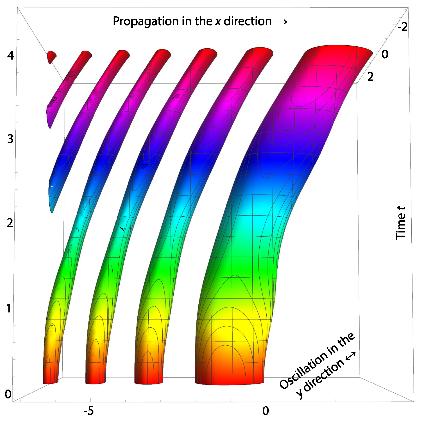
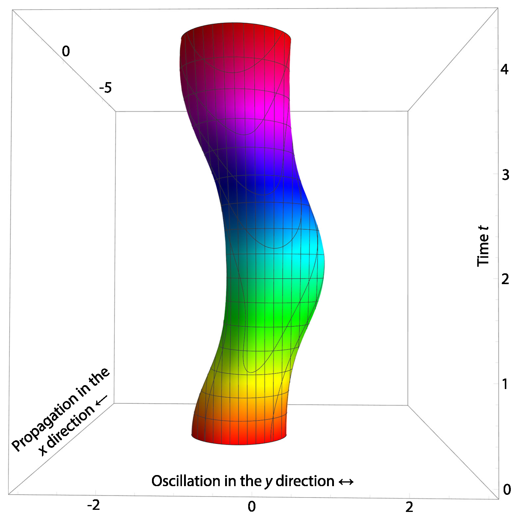
The Airy propagating oscillation is damped, but there is no spreading; it remains diffraction-free. Despite the amplitude decrease during propagation, the signal can be easily reconstructed. These statements are not the same as saying that the wave remains coherent. It means that it can be recognized in its attenuated form, at least for a while, and we can trace it back to the original shape. It seems a promising opportunity in the fields of information storage and transfer. We follow the propagating waves in Figure 1, Figure 2, Figure 3 and Figure 4. (The applied parameters are (in dimensionless units): $B=0.9$; $h=1$; $m=1$; $\gamma =0.75$; $\omega =1.5$; $\lambda =0.06$.) The non-damped propagation is visible from two different views. The typical Airy beam can be identified from the front view in Figure 1. As it can be recognized, the shape (the structure) of the beam is preserved during the time evolution. The oscillation of the beam (train wave) can be seen from the face view in Figure 2. In this case, due to covering, we see only the first element of the beam. The wavefront is coming towards us. The elapsed time is shown on the vertical axis.

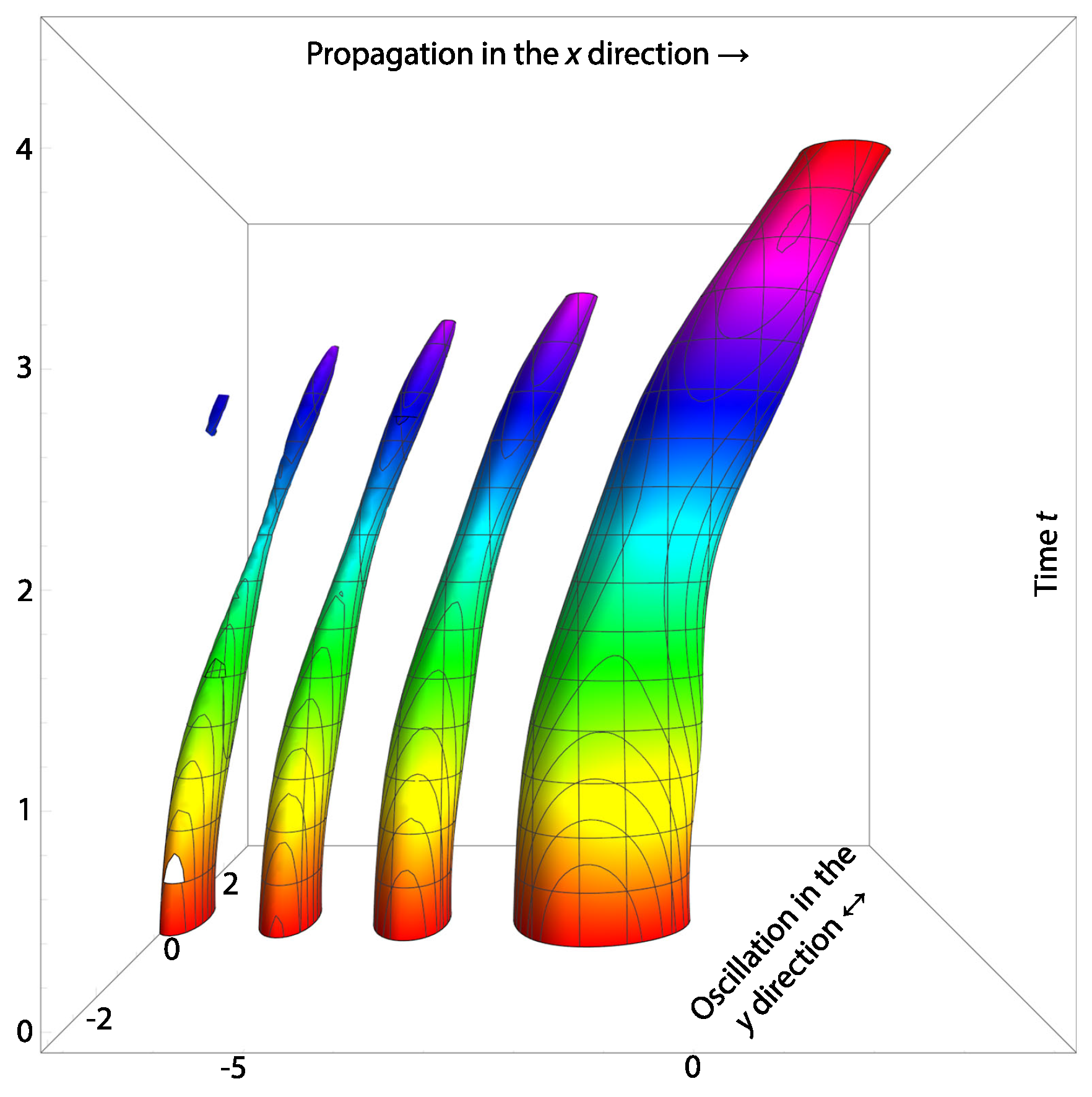
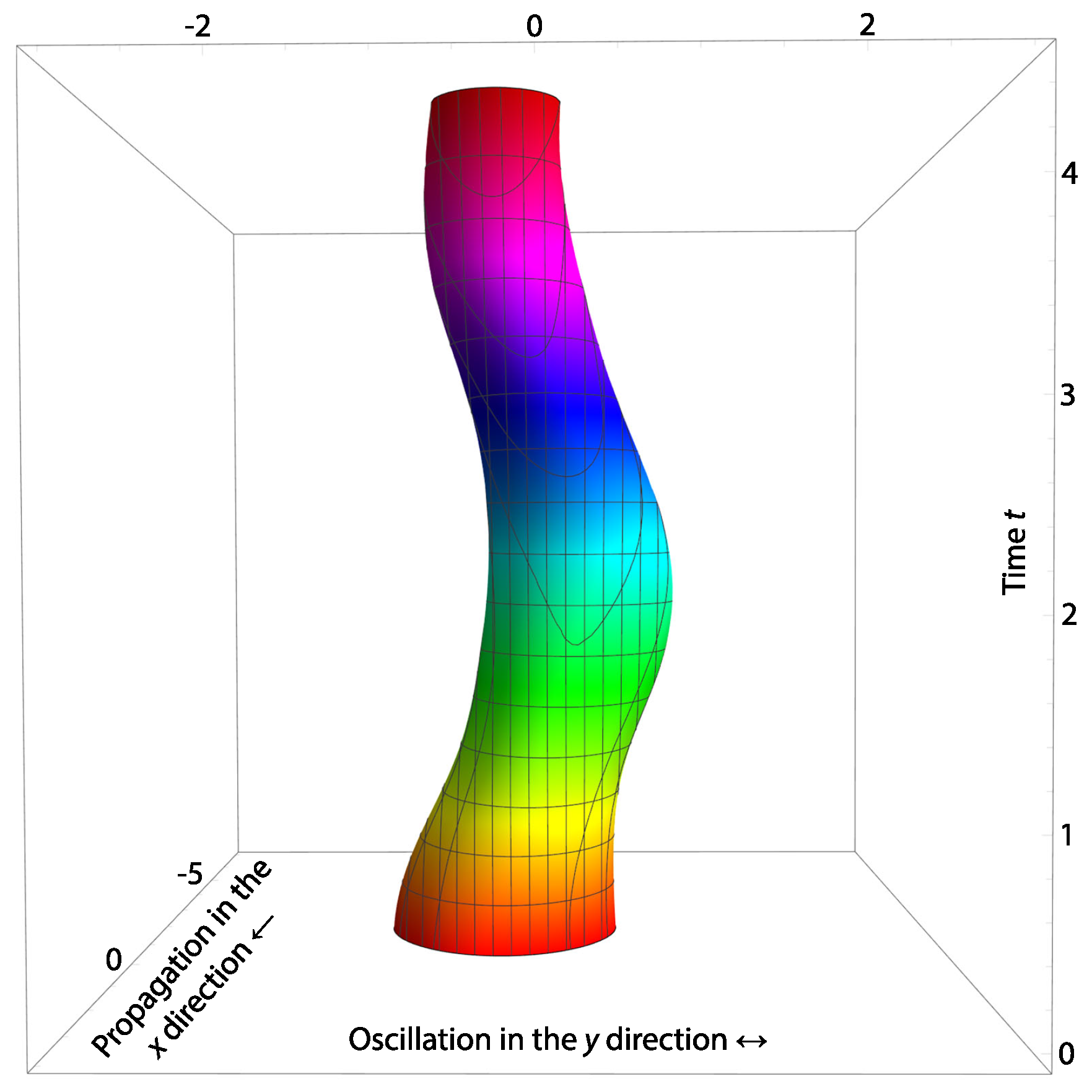
The damping of the Airy wave packet is observable from the thinner wave components. However, there is no spreading-out motion, as Figure 3 (front view) and Figure 4 (side view) show. We can continuously identify the remaining structure of the beam. It means that the involved information is always recognizable during the transfer. The damping itself is not equal to the total information loss. We can amplify the attenuating amplitude to its original value. Finally, it seems we can recover the initial information or, at least, recognize it. As we mentioned previously, the presented transverse wave is a superposition of two damped propagation modes. Moreover, since the Gaussian solution is also a part of Equation (41), their combination gives a physically realistic movement.

The signal reconstruction is of fundamental importance in information transfer. In spin relaxation-based processes, the Loschmidt echo [6,7] seems promising in restoring the original signal. This is a process in which the initial state is recoverable quite well. Hopefully, by combining it with the presented ideas, the loss in information can be decreased, and state recovery can be achieved effectively. It is a great challenge for the future.

Countless open questions remain regarding damped quantum mechanical wave states and signal reconstruction. Nevertheless, there are similar efforts in the literature regarding the minimization of transmission loss and channel instability [60,61].

6. Conclusions

The application of the potential-based canonical quantization procedure can be extended to damped transversal mechanical waves. We show that the structure of the canonical variables, momenta, and coordinates is flexible enough to separate the oscillating $(P_{1y},P_{2y},Q_{1y},Q_{2y})$ and the propagating $(P_{1x},P_{2x},Q_{1x},Q_{2x})$ motions. Via the Fourier-transformed canonical quantities, we achieve the operator calculus. Finally, the particular property of the Hamiltonian, namely, its zero value, enables us to formulate the related damped transversal wave equation. (Since, in our method, the Lagrangian does not depend on time explicitly, the Hamiltonian must be constant. In the case of dissipative processes, this requirement does not seem to be evident. However, the zero-valued property of the Hamiltonian ensures this requirement and also helps to avoid the unlimited and unstable solutions.) The obtained state equation describes the damping in such a way that it pertains to the oscillator and the transversal motion in the same interaction. It reflects the physically relevant situation where there is only one damping effect on the propagation. The solution to the state equation can be expressed as the product of the quantum oscillator (relating to the path integral method with the shape-changing formation), the transversal motion (Gaussian or Airy), and the exponentially time-decreasing factor. We show that there are two possibilities for the transversal solutions. (1) One of these is the Gaussian solution, where the signal is spreading; together with the damping, the carried information tends to zero over time. The damping indicates such a loss in the signal that restoration is impossible in this scenario. (2) The other possibility is the Airy wave train (beam). This solution is non-spreading, diffraction-free, and shape-preserving, despite the damping. The amplitude of the signal is decreasing. However, the original signal content might be recovered through a non-linear amplifying process. The process of amplification does not have to affect the structure of the signal. The discussed wave propagation mode is promising for long-range quantum signal transfer. It is an open question of how to apply the presented method for other types of transfer, like spin waves, charge/spin density waves, and other related transfers. This research may be necessary for information technology applications.

References

- Márkus, F.; Gambár, K. Minimum Entropy Production Effect on a Quantum Scale. Entropy 2021, 23, 1350. [Google Scholar] [CrossRef] [PubMed]
- Ithier, G.; Collin, E.; Joyez, P.; Meeson, P.J.; Vion, D.; Esteve, D.; Chiarello, F.; Shnirman, A.; Makhlin, Y.; Schriefl, J.; et al. Decoherence in a Superconducting Quantum Bit Circuit. Phys. Rev. B 2005, 72, 134519. [Google Scholar] [CrossRef]
- Schoelkopf, R.J.; Girvin, S.M. Wiring up Quantum Systems. Nature 2008, 451, 664–669. [Google Scholar] [CrossRef] [PubMed]
- Márkus, B.G.; Szirmai, P.; Edelthalhammer, K.F.; Eckerlein, P.; Hirsch, A.; Hauke, F.; Nemes, N.M.; Chacón-Torres, J.C.; Náfrádi, B.; Forró, L.; et al. Ultralong Spin Lifetime in Light Alkali Atom Doped Graphene. ACS Nano 2020, 14, 7492–7501. [Google Scholar] [CrossRef] [PubMed]
- Márkus, B.G.; Gmitra, M.; Dóra, B.; Csősz, G.; Fehér, T.; Szirmai, P.; Náfrádi, B.; Zólyomi, V.; Forró, L.; Fabian, J.; et al. Ultralong 100 ns Spin Relaxation Time in Graphite at Room Temperature. Nat. Commun. 2023, 14, 2831. [Google Scholar] [CrossRef]
- Csősz, G.; Dóra, B.; Simon, F. Entropy in Spin Relaxation, Spintronics, and Magnetic Resonance. Phys. Status Solidi B 2020, 257, 2000301. [Google Scholar] [CrossRef]
- Csősz, G.; Szolnoki, L.; Kiss, A.; Dóra, B.; Simon, F. Generic Phase Diagram of Spin Relaxation in Solids and the Loschmidt Echo. Phys. Rev. Res. 2020, 2, 033058. [Google Scholar] [CrossRef]
- Mahmoud, A.; Ciubotaru, F.; Vanderveken, F.; Chumak, A.V.; Hamdioui, S.; Adelmann, C.; Cotofana, S. Introduction to Spin Wave Computing. J. Appl. Phys. 2020, 128, 161101. [Google Scholar] [CrossRef]
- Palma, G.M.; Suominen, K.-A.; Ekert, A.K. Quantum Computers and Dissipation. Proc. R. Soc. A 1996, 452, 567–584. [Google Scholar]
- Beke, D.; Valenta, J.; Károlyházy, G.; Lenk, S.; Czigány, Z.; Márkus, B.G.; Kamarás, K.; Simon, F.; Gali, G. Room-Temperature Defect Qubits in Ultrasmall Nanocrystals. J. Phys. Chem. Lett. 2020, 11, 1675–1681. [Google Scholar] [CrossRef]
- Zhou, X.; Koolstra, G.; Zhang, X.; Yang, G.; Han, X.; Dizdar, B.; Li, X.; Divan, R.; Guo, W.; Murch, K.W.; et al. Single Electrons on Solid Neon as a Solid-State Qubit Platform. Nature 2022, 605, 47–50. [Google Scholar] [CrossRef]
- Kollarics, S.; Simon, F.; Bojtor, A.; Koltai, K.; Klujber, G.; Szieberth, M.; Márkus, B.G.; Beke, D.; Kamarás, K.; Gali, A.; et al. Ultrahigh Nitrogen-Vacancy Center Concentration in Diamond. Carbon 2022, 188, 393–400. [Google Scholar] [CrossRef]
- Haken, H. Laser Theory, Encyclopedia of Physics; Springer: Berlin/Heidelberg, Germany; New York, NY, USA, 1970; Volume XXV/2c. [Google Scholar]
- Haake, F. Springer Tracts Modern Physics; Springer: Berlin/Heidelberg, Germany; New York, NY, USA, 1973; Volume 66, pp. 98–168. [Google Scholar]
- Caldirola, P. Forze non Conservative Nella Meccanica Quantistica. Il Nuovo C. 1941, 18, 393–400. [Google Scholar] [CrossRef]
- Kanai, E. On the Quantization of the Dissipative Systems. Prog. Theor. Phys. 1948, 3, 440–442. [Google Scholar] [CrossRef]
- Dekker, H. Classical and Quantum Mechanics of the Damped Harmonic Oscillator. Phys. Rep. 1981, 80, 1–110. [Google Scholar] [CrossRef]
- Dittrich, W.; Reuter, M. Classical and Quantum Dynamics; Springer: Berlin/Heidelberg, Germany, 1996. [Google Scholar]
- Weiss, U. Quantum Dissipative Systems; World Scientific: Singapore, 2012. [Google Scholar]
- Leggett, A.J. Quantum Tunneling in the Presence of an Arbitrary Linear Dissipation Mechanism. Phys. Rev. B 1984, 30, 1208. [Google Scholar] [CrossRef]
- Caldeira, A.O.; Neto, A.H.C.; de Carvalho, T.O. Dissipative Quantum Systems Modeled by a Two-level-reservoir Coupling. Phys. Rev. B 1993, 48, 13974. [Google Scholar] [CrossRef] [PubMed]
- da Costa, M.R.; Caldeira, A.O.; Dutra, S.M.; Westfahl, H. Exact Diagonalization of Two Quantum Models for the Damped Harmonic Oscillator. Phys. Rev. A 2000, 61, 022107. [Google Scholar] [CrossRef]
- Choi, J.R. Analysis of Quantum Energy for Caldirola–Kanai Hamiltonian Systems in Coherent States. Results Phys. 2013, 3, 115–121. [Google Scholar] [CrossRef]
- Bagarello, F.; Gargano, F.; Roccati, F. A No-Go Result for the Quantum Damped Harmonic Oscillator. Phys. Lett. A 2019, 383, 2836–2838. [Google Scholar] [CrossRef]
- Bateman, H. On Dissipative Systems and Related Variational Principles. Phys. Rev. 1931, 38, 815. [Google Scholar] [CrossRef]
- Risken, H. The Fokker-Planck Equation: Methods of Solution and Applications, 2nd ed.; Springer: Berlin/Heidelberg, Germany, 1989; Appendix A.4; pp. 425–428. [Google Scholar]
- Serhan, M.; Abusini, M.; Al-Jamel, A.; El-Nasser, H.; Rabei, E.M. Quantization of the Damped Harmonic Oscillator. J. Math. Phys. 2018, 59, 082105. [Google Scholar] [CrossRef]
- Serhan, M.; Abusini, M.; Al-Jamel, A.; El-Nasser, H.; Rabei, E.M. Response to Comment on ‘Quantization of the Damped Harmonic Oscillator’. J. Math. Phys. 2019, 60, 094101. [Google Scholar] [CrossRef]
- El-Nabulsi, R.A. Path Integral Method for Quantum Dissipative Systems with Dynamical Friction: Applications to Quantum Dots/Zero-dimensional Nanocrystals. Superlattices Microstruct. 2020, 144, 106581. [Google Scholar] [CrossRef]
- Szegleti, A.; Márkus, F. Dissipation in Lagrangian Formalism. Entropy 2020, 22, 930. [Google Scholar] [CrossRef]
- Márkus, F.; Gambár, K. A Potential-Based Quantization Procedure of the Damped Oscillator. Quantum Rep. 2022, 4, 390–400. [Google Scholar] [CrossRef]
- Abers, E.S. Quantum Mechanics; Pearson Education: Upper Saddle River, NJ, USA, 2004. [Google Scholar]
- Airy, G.B. Tides and Waves. In Encyclopaedia Metropolitana (1817–1845), Mixed Sciences. Vol. 3; Rose, H.J., Rose, H.J., Smedley, E., Eds.; B. Fellowes: London, UK, 1841; pp. 241–396. [Google Scholar]
- Siviloglou, G.A.; Broky, J.; Dogariu, A.; Christodoulides, D.N. Observation of Accelerating Airy Beams. Phys. Rev. Lett. 2007, 99, 213901. [Google Scholar] [CrossRef]
- Siviloglou, G.A.; Christodoulides, D.N. Accelerating Finite Energy Airy Beams. Opt. Lett. 2007, 32, 979–981. [Google Scholar] [CrossRef]
- Kondakci, H.E.; Abouraddy, A.F. Diffraction-free Space–Time Light Sheets. Nat. Photonics 2017, 11, 733–740. [Google Scholar] [CrossRef]
- Kondakci, H.E.; Abouraddy, A.F. Airy Wave Packets Accelerating in Space-Time. Phys. Rev. Lett. 2018, 120, 163901. [Google Scholar] [CrossRef]
- Rozenman, G.G.; Zimmermann, M.; Efremov, M.A.; Schleich, W.P.; Shemer, L.; Arie, A. Amplitude and Phase of Wave Packets in a Linear Potential. Phys. Rev. Lett. 2019, 122, 124302. [Google Scholar] [CrossRef]
- Hall, L.A.; Yessenov, M.; Abouraddy, A.F. Arbitrarily Accelerating Space-Time Wave Packets. Opt. Lett. 2022, 47, 694–697. [Google Scholar] [CrossRef]
- Grosman, D.; Sheremet, N.; Pavlov, I.; Karlovets, D. Elastic Scattering of Airy Electron Packets on Atoms. Phys. Rev. A 2023, 107, 062819. [Google Scholar] [CrossRef]
- Rozenman, G.G.; Bondar, D.I.; Schleich, W.P.; Shemer, L.; Arie, A. Observation of Bohm Trajectories and Quantum Potentials of Classical Waves. Phys. Scr. 2023, 98, 044004. [Google Scholar] [CrossRef]
- Ostrogradski, M. Mémoires sur les équations différentielles, relatives au problème des isopérimètres. Mem. Ac. St. Petersbourg 1850, 6, 385. [Google Scholar]
- Dysthe, K.B. Note on a Modification to the Nonlinear Schrödinger Equation for Application to Deep Water Waves. Proc. R. Soc. Lond. A 1979, 369, 105–114. [Google Scholar]
- Craig, W.; Guyenne, P.; Sulem, C. A Hamiltonian Approach to Nonlinear Modulation of Surface Water Waves. Wave Motion 2010, 47, 552–563. [Google Scholar] [CrossRef]
- Guyenne, P.; Kairzhan, A.; Sulem, C.; Xu, B. Spatial Form of a Hamiltonian Dysthe Equation for Deep-Water Gravity Waves. Fluids 2021, 6, 103. [Google Scholar] [CrossRef]
- Márkus, F.; Gambár, K. Derivation of the Upper Limit of Temperature from the Field Theory of Thermodynamics. Phys. Rev. E 2004, 70, 055102(R). [Google Scholar] [CrossRef] [PubMed]
- Márkus, F.; Gambár, K. Symmetry Breaking and Dynamic Transition in the Negative Mass Term Klein–Gordon Equation. Symmetry 2024, 16, 144. [Google Scholar] [CrossRef]
- Gambár, K.; Márkus, F. Hamilton-Lagrange Formalism of Nonequilibrium Thermodynamics. Phys. Rev. E 1994, 50, 1227. [Google Scholar] [CrossRef]
- Gambár, K.; Rocca, M.C.; Márkus, F. A Repulsive Interaction in Classical Electrodynamics. Acta Polytechn. Hung. 2020, 17, 175–189. [Google Scholar] [CrossRef]
- Jackson, J.D. Classical Electrodynamics; John Wiley & Sons.: Hoboken, NJ, USA, 1999. [Google Scholar]
- Courant, R.; Hilbert, D. Methods of Mathematical Physics; Interscience: New York, NY, USA, 1966. [Google Scholar]
- Smilga, A.V. Comments on the Dynamics of the Pais–Uhlenbeck Oscillator. SIGMA 2009, 5, 017. [Google Scholar] [CrossRef]
- Motohashi, H.; Suyama, T. Third Order Equations of Motion and the Ostrogradsky Instability. Phys. Rev. D 2015, 91, 085009. [Google Scholar] [CrossRef]
- Razavy, M. Classical and Quantum Dissipative Systems; Imperial College Press: London, UK, 2005; p. 129. [Google Scholar]
- Halász, G.J.; Vibók, Á. Comparison of the Imaginary and Complex Absorbing Potentials Using Multistep Potential Method. Int. J. Quantum Chem. 2003, 92, 168–173. [Google Scholar] [CrossRef]
- Muga, J.G.; Palao, J.P.; Navarro, B.; Egusquiza, I.L. Complex Absorbing Potentials. Phys. Rep. 2004, 395, 357–426. [Google Scholar] [CrossRef]
- Márkus, B.G.; Márkus, F. Quantum Particle Motion in Absorbing Harmonic Trap. Indian J. Phys. 2016, 90, 441–446. [Google Scholar] [CrossRef]
- Naqvi, K.R.; Waldenstrøm, S. Revival, Mirror Revival and Collapse may Occur even in a Harmonic Oscillator Wave Packet. Phys. Scr. 2000, 62, 12. [Google Scholar] [CrossRef]
- Berry, M.V.; Balazs, N.L. Nonspreading Wave Packets. Am. J. Phys. 1979, 47, 264–267. [Google Scholar] [CrossRef]
- Chen, K.C.; Dhara, P.; Heuck, M.; Lee, Y.; Dai, W.; Guha, S.; Englund, D. Zero-Added-Loss Entangled-Photon Multiplexing for Ground- and Space-Based Quantum Networks. Phys. Rev. Appl. 2023, 19, 054029. [Google Scholar] [CrossRef]
- Bersin, E.; Sutula, M.; Huan, Y.Q.; Suleymanzade, A.; Assumpcao, D.R.; Wei, Y.-C.; Stas, P.-J.; Knaut, C.M.; Knall, E.N.; Langrock, C.; et al. Telecom Networking with a Diamond Quantum Memory. PRX Quantum 2024, 5, 010303. [Google Scholar] [CrossRef]
Figure 1.
Non-damped oscillating−traveling Airy wave, front view. The translational propagation is in the –direction (from left to right); the oscillation is along the –axis (on the plane). The third coordinate is the time scale, t. The same color pertains to the same moment in time.
Figure 2.
Non-damped oscillating−traveling Airy wave, side view. The translational propagation is coming towards us; the oscillation is along the –axis (on the plane). The third coordinate is the time scale, t. The same color pertains to the same moment in time.
Figure 3.
Damped oscillating−traveling Airy wave, front view. The translational propagation is in the –direction (from left to right); the oscillation is along the –axis (on the plane). The third coordinate is the time scale, t. The same color pertains to the same moment in time. The dissipation (information loss) can be recognized from the narrowing of the beam’s cross-section (from the bottom to the top).
Figure 4.
Damped oscillating−traveling Airy wave, side view. The translational propagation is coming towards us; the oscillation is along the –axis (on the plane). The third coordinate is the time scale, t. The same color pertains to the same moment in time. The damping of the oscillation can be recognized well from the narrowing of the beam’s cross-section (from the bottom to the top).
Disclaimer/Publisher’s Note: The statements, opinions and data contained in all publications are solely those of the individual author(s) and contributor(s) and not of MDPI and/or the editor(s). MDPI and/or the editor(s) disclaim responsibility for any injury to people or property resulting from any ideas, methods, instructions or products referred to in the content. |
© 2024 by the authors. Licensee MDPI, Basel, Switzerland. This article is an open access article distributed under the terms and conditions of the Creative Commons Attribution (CC BY) license (https://creativecommons.org/licenses/by/4.0/).
Share and Cite
MDPI and ACS Style
Márkus, F.; Gambár, K. Quantized Approach to Damped Transversal Mechanical Waves. Quantum Rep. 2024, 6, 120-133. https://doi.org/10.3390/quantum6010009
AMA Style
Márkus F, Gambár K. Quantized Approach to Damped Transversal Mechanical Waves. Quantum Reports. 2024; 6(1):120-133. https://doi.org/10.3390/quantum6010009
Chicago/Turabian StyleMárkus, Ferenc, and Katalin Gambár. 2024. "Quantized Approach to Damped Transversal Mechanical Waves" Quantum Reports 6, no. 1: 120-133. https://doi.org/10.3390/quantum6010009