
Topological Properties of the 2D 2-Band System with Generalized W-Shaped Band Inversion


Department of Physics, Faculty of Science, University of Zagreb, Bijenička 32, 10000 Zagreb, Croatia
*
Author to whom correspondence should be addressed.
†
These authors contributed equally to this work.
Quantum Rep. 2022, 4(4), 476-485; https://doi.org/10.3390/quantum4040034
Submission received: 26 September 2022
/
Revised: 25 October 2022
/
Accepted: 29 October 2022
/
Published: 2 November 2022
Abstract
:We report the topological properties, in terms of the Berry phase, of the 2D noninteracting system with electron–hole band inversion, described by the two-band generalized analogue of the low-energy Bernevig–Hughes–Zhang Hamiltonian, yielding the W-shaped energy bands in the form of two intersecting cones with the gap along the closed continuous loop. We identify the range of parameters where the Berry phase attains qualitatively different values: (a) the integer multiplier of , (b) the integer multiplier of , and (c) the nontrivial value between the latter two, which depends on the system parameters. The system thus exhibits the anomalous quantum Hall effect associated with the nontrivial geometric phase, which is presumably tunable through the choice of parameters at hand.
1. Introduction
The Berry phase [1] was introduced at least conceptually for the first time most likely in the 1950s in D. Bohm’s Quantum Theory [2], Ch. 20, Sec. 1 in equation 8, as the geometric phase accumulated in the wave function during the cyclic adiabatic change of parameters in the Hamiltonian; today, it still grasps the focus of interest of the modern physics, particularly in the fields of condensed matter and optics [3]. The concept of nontrivial topological properties of the wave function is important not only from the fundamental point of view of the general quantum mechanics but also from the experimental and technological point of view. The topological insulators [4] and quantum Hall effect (QHE) [5,6] are just some of the most well-known examples of real systems with the above-mentioned effects experimentally observed. Furthermore, the anyons, firstly suggested by F. Wilcek as the composite particles consisting of the electric charge moving in the 2D plane around the infinite magnetic flux tube perpendicular to it [7], are objects satisfying neither fermionic nor bosonic statistics. In turn, the phase in the wave function, accumulated by braiding the two of them, is neither zero (bosons) nor (fermions) but some real number between the two instead, reflecting the nontrivial topology of the wave function. The fundamental requirement to be able to achieve such a nontrivial braiding is the two-dimensionality (2D) of the system. So far, the only experimentally realized system exhibiting anyons in the field of solid-state physics is the fractional QHE [8,9], which is emerging due to electron–electron interactions. The extra efforts to realize anyons in different systems, especially the so-called non-Abelian ones, is also motivated by their potential application for quantum computation [10]. Some of these efforts are directed at finding the systems in which anyons may emerge in the absence of interactions (e.g., the electron–electron interaction) but solely due to the special topology of the wave function, resulting from diagonalization of the Hamiltonian containing parameters that can be controlled from the outside [11], the realization of which is still an open question.
We analyze the topological properties of the 2D system with inverted electron and hole bands. The band inversion and so-called “conical intersections” [12] are practically paradigmatic prerequisites for the nontrivial topological properties and onset of the topological insulators. Although the full scale of mechanisms leading to the band inversion is not fully known yet, usually, the spin–orbit interaction in the solid state is used as its main generator. The quest to generate the intrinsic QHE state, as an intrinsic property of the system without the external magnetic field (so-called anomalous QHE) [13], has been continued since Haldane’s proposal [14], its experimental realizations [15], as the important topic of modern solid-state physics and material science through the design of new topological materials. Here, we shall not discuss the mechanisms leading to the band inversion. We shall start with the Hamiltonian already possessing that feature and explore its properties. The system under consideration features the W-shaped bands with rotational symmetry (the so-called “Witch’s hat” form created by the two oppositely oriented intersecting cones with a gap created along the circular line of intersection). It is in essence the two-band derivative of the low-energy Bernevig–Hughes–Zhang Hamiltonian (BHZ) [16] for the 2D system, which is sometimes called the “half BHZ model”, leading to the modified Dirac equation [17], which we generalize in terms of the number of parameters presumably tunable by the external influence such as electric field, mechanical strain, etc. The results indicate regions of parameters for which the Berry phase can achieve different nontrivial values; i.e., we find regions in the parameter space with the nontrivial Berry phase characterized by the integer multiplier of and of as well as the region where the Berry phase attains the nontrivial value between the latter two depending on the parameters in the Hamiltonian. Likewise, the anomalous QHE determined by it emerges, possessing the corresponding nonstandard properties.
2. Methods
2.1. The Model
The low-energy Hamiltonian of the 2D two-band system under consideration, in the basis of the plane waves characterizes by the 2D wave vector , reads
where is one of the parameters determining the band gap, and parameters are positive integers. In particular, m describes different possible initial electron dispersions such as linear, parabolic etc., while n describes the possibility of introducing more general topology beyond simple conical band intersections. The case (and ) is also covered by the result, but it leads to the trivial topology; thus, we shall comment on it at the end only for the sake of completeness. Here, () stand for positive parameters giving, multiplied with (), dimension of energy, e.g., for , are the Fermi velocity parameters such as for graphene, for example; for , are the effective mass () parameters such as for the free electron gas, etc.
Using the in-plane rotational symmetry of the problem, i.e., using the polar coordinates and , in which , and expressing energy E in units of , i.e., consequently scaling the Hamiltonian in the same way, i.e., , we can write the Hamiltonian (1) in the convenient form for analytical analysis
where and are the control parameters of the model, together with the corresponding exponents n and m. It is straightforward to diagonalize the Hamiltonian (2). The eigen-states, i.e., the electronic energy bands, are
where the sign “+” stands for the conduction (or electron) band, and sign “−” stands for the valence (or hole) band. The bands are shown schematically in Figure 1 for several choices of parameters.
The (normalized) eigen-vectors in the plane wave basis in polar coordinates, corresponding to the eigen-states (3), are
2.2. The Berry Phase
Knowing the eigen-vectors, we can calculate the Berry connection in polar coordinates, where
playing the role of the “Berry (vector) potential”, or synthetic gauge field generated by the “topological charge” located in the origin. Performing the partial differentiation and the straightforward algebra, we obtain
The Berry phase for each band is then calculated as the contour integral of along the path encircling the “topological charge” in the origin. In the case of standard solid-state systems at the lattice, that path encircles the Brillouin zone, being the natural boundary along which the derivative of the wave function vanishes due to the periodicity condition. The topology of the 2D Brillouin zone is the one of the torus, granting the integer (or trivial, i.e., zero) TKNN invariant, also called the Chern number, in the standard noninteracting systems, thus reflecting its topological nature [18]. The presented model is approximate in the sense that it is continuous; we modeled just the vicinity of the conical intersection without full periodicity conditions of the lattice (so-called low-energy Hamiltonian). Thus, the path encircling the “topological charge” in the origin should be taken in the limit . This reflects its geometric instead of pure topological nature (such as for the pure Dirac cone in graphene, for example). Therefore, the Berry phase is
which transforms, after inserting the expression for the Berry connection (6) and taking the integral, into
and, taking the limit, we finally obtain
2.3. The Anomalous QHE
Another way to address the intrinsic QHE originating solely from the band topology is the calculation of the electrical conductivity tensor within the adiabatic approximation, namely its off-diagonal element that accounts for the Hall conductivity. The contribution in the case of the full band accounts exactly for the QHE as illustrated in detail in early works of Streda, Kohomoto and others [19,20,21]. The simplest way is to calculate the average of the, say, x-component of the current operator as the response to the perpendicular electric field introduced through the time-dependent gauge, i.e., the vector potential of the form , where is the perpendicular component of electric field, and t is time.
The current operator is defined by the expression
where is the Hamiltonian of the system, and the Hall conductivity is defined as the response function, i.e., . The Hall conductivity in this case, per state with energy in the, by assumption, fully occupied band, is given by the well-known Kubo formula
In our case with two bands and , Equation (11), after summing up the contributions per states in the band, reduces to the expression for the Hall conductivity per band [22]
where we calculated it per unit area. To pursue this quest, one needs to calculate the current vertices
where accounts for the Cartesian component and are the indices denoting (row, column) the corresponding matrix elements. are elements of the -dependent unitary matrix
determined by the condition , where is the diagonal eigenvalue matrix and
Taking it into account, the current vertices (13) read
for the intraband () and interband () case, respectfully.
We illustrate the procedure and the result for the particular problem, using the Hamiltonian (1) for the case . Having , , and , we calculate the interband current vertices for our two-band system with the valence band () and conduction band ()
for which , and where the spectrum, appearing in the expression, is .
The (quantum) Hall conductivity of the system with a fully occupied valence band () and empty conduction band (), with , is given by the expression
3. Results
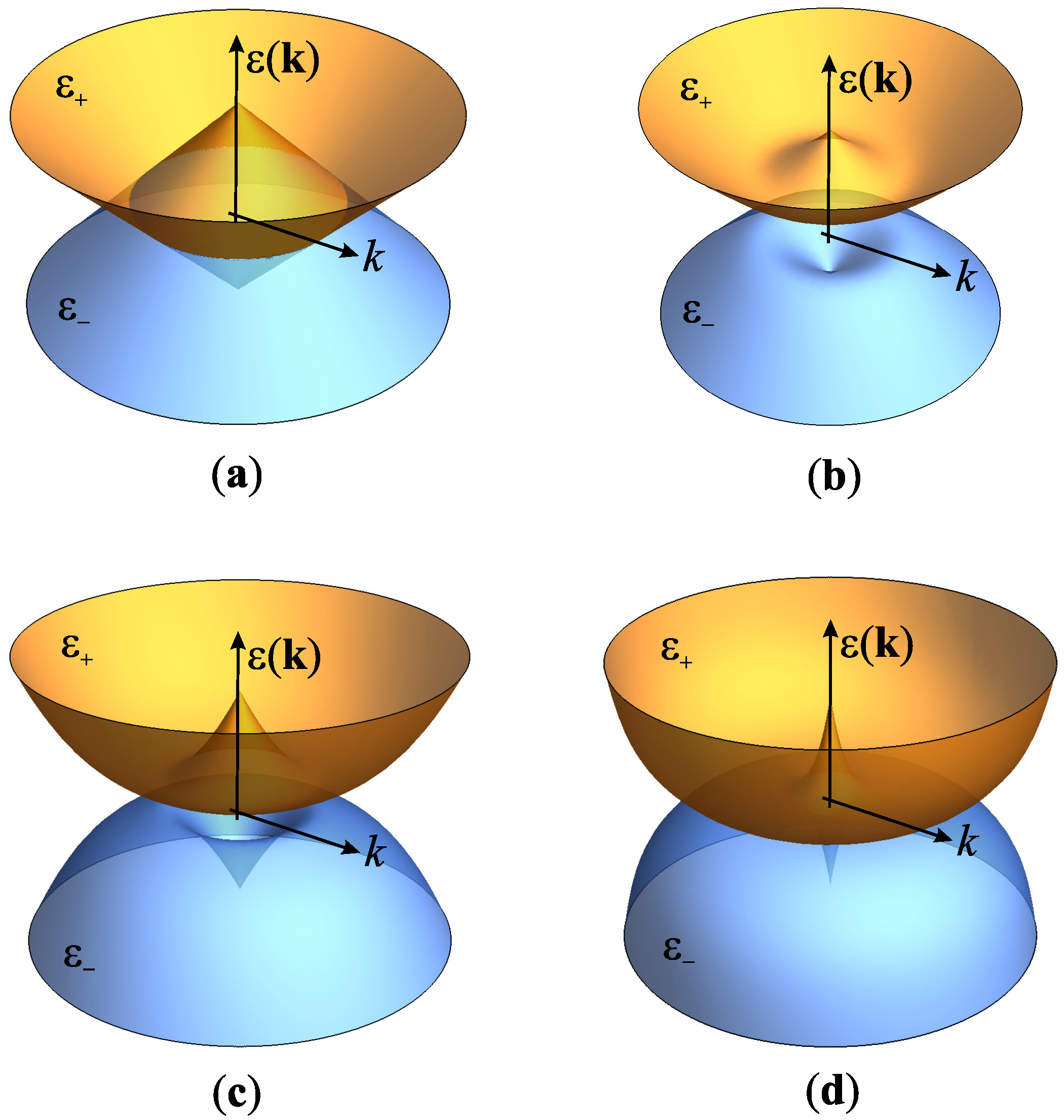
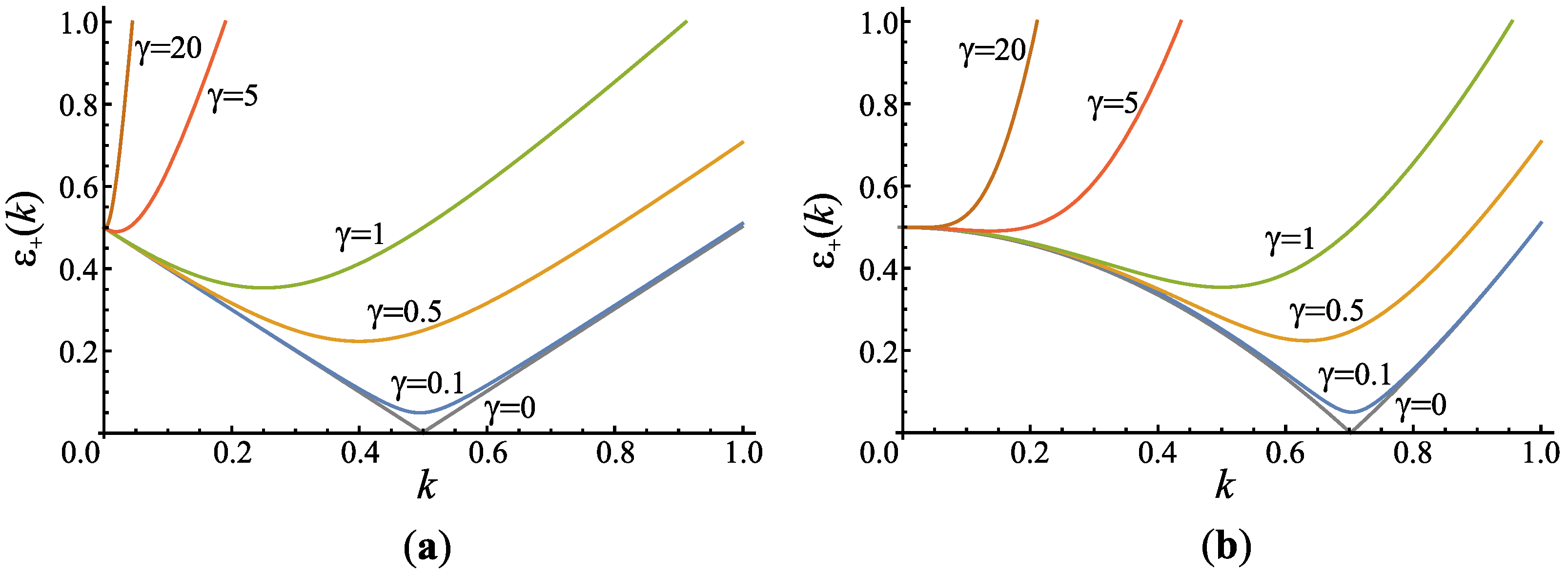
The most natural way to analyze the obtained results is to start with the properties of the electron energy bands (3) which also reflect the topological properties, depending on parameters. The band structure, depending on the characteristic choices of parameters, is shown in Figure 2. In principle, the energy bands have two intersecting cones with a gap opened between them along the circular intersecting line (we call it “the nodal ring”). The tips of the protruding cones are located symmetrically, beyond and beneath the origin, at the distance equal to . The circular nodal ring, giving the W-shape (or “Mexican hat-shape”, depending on n, m), shrinks in radius as increases, but it is preserved up to the limit .
For the case , the radius of the nodal ring is , and the real band gap, i.e., the vertical distance between the lower and upper band, along the nodal ring is equal to (or in the original units of energy). In the general case , one needs to solve the equation for and insert it into expression (3) to find the value of the gap .
The Berry phase of the system is a sum of the contributions of all occupied bands. We consider the case with only the lower band (“−”) fully occupied and upper band (“+”) empty. Then, the Berry phase of the system is equal to , i.e.,
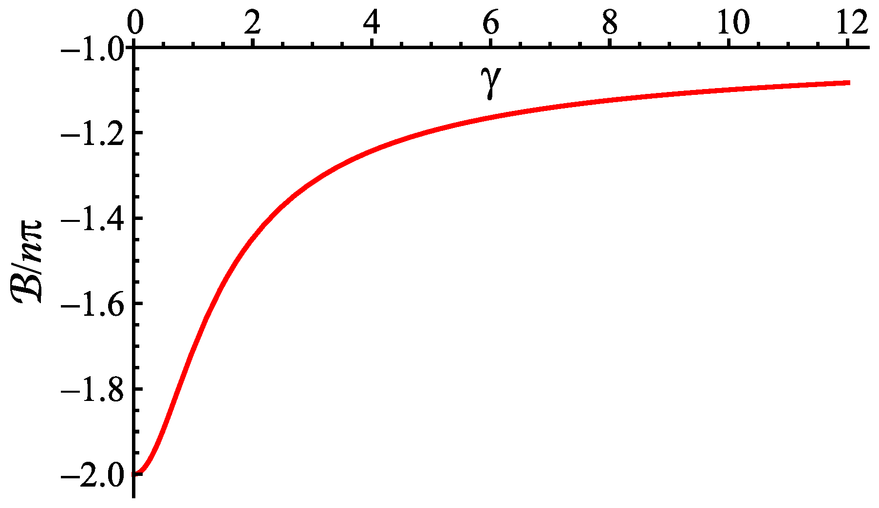
opening the possibility of different classes of nontrivial results dependent on the system parameters (but not on the scaling of energy). It is essential to stress that this result holds as long as we have two distinct bands, i.e., until the gap closes. Basically, the result exhibits three main classes depending on the relation of n and m: (a) if , attains the value ; if , attains the value ; if , attains the value between and depending on . We show the Berry phase for the case in Figure 3. Apparently, as , the band gap closes and . In the opposite case , the W-shape of the band is lost, yielding the value .
The anomalous QHE is confirmed also by the “electrodynamical approach”, i.e., by the calculation of the Hall conductivity in the gapped state using the interband current vertices. The result (18), obtained for the case , can be easily generalized using the analogous straightforward procedure for the case of general . It yields the result , where
The conductivity appears in the units of conductivity quanta multiplied by the dimensionless quantity which appears as the “winding number” equal to the Berry phase divided by , therefore being in accordance with Equation (19). In the next section, we shall discuss when it may have the meaning of the topological invariant known as the Chern number.
4. Discussion
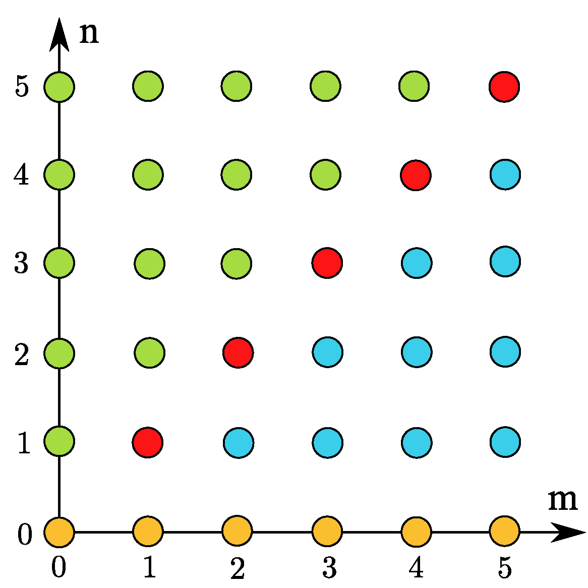
Physical systems featuring different topological properties are nowadays well categorized in terms of classes of corresponding topological invariants depending on the symmetries that the system possesses [23]. The general topological properties of conical intersections, as generators of nontrivial synthetic gauge fields, and inverted bands are rather well-understood. The interesting upgrade to that established picture is to find a way how to tune or violate certain assumptions, upon which the symmetry classes are built, through the change of parameters, and then track the transitions between the topological phases. The model that we analyze is symmetric with respect to the time reversal; it is the low-energy approximation which reflects topological properties of the single (generalized) conical intersection, which is expressed in terms of the “winding number” given by Equation (20). The character of the conical intersection, expressed by , is determined by the system parameters m, n and , yielding the topological phase diagram with two phases and the unusual boundary between them—Figure 4.
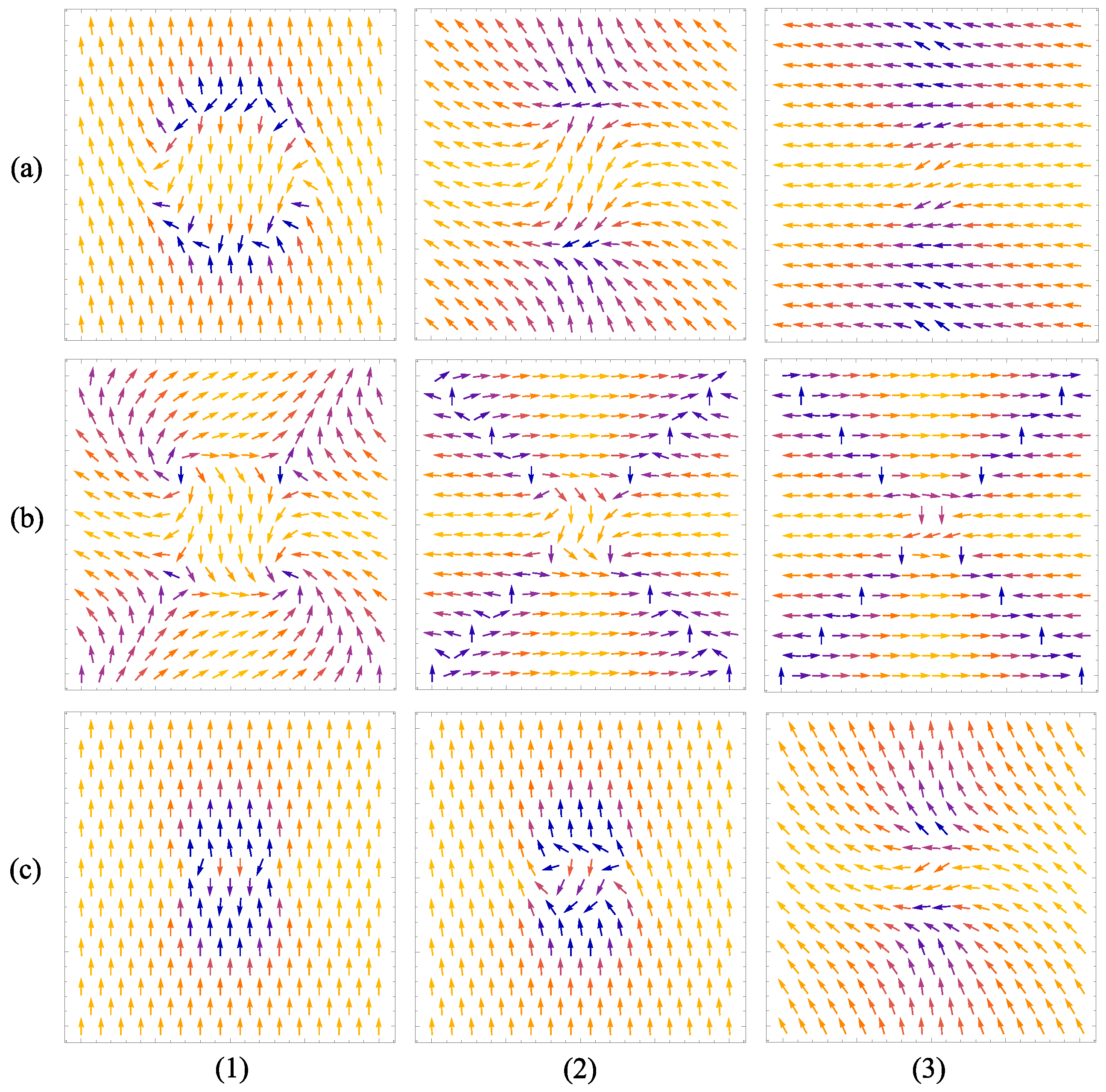
The result reproduces, for example, the result for the modified Dirac equation, [17], taking parameters and , or the point of simple “massive graphene” [24] with for and , or trivial insulator with for , (e.g., , case is considered in Ref. [25]), etc. However, the analyzed system goes qualitatively beyond that. Apart from the trivial phase () for , in the case of the nonzero n, the “winding number” remains such for all . It attains the value for all . Finally, for all , . As a result of the lack of other effective means of visualization, we illustrate the effect of topology, “encoded” into the wave function (4), on the spin operator , by calculating the vector field having the expected values of and operators as its components, i.e.,
as depicted in Figure 5 (the topologically trivial case would have all spins directed “upwards”).
To apply the presented results to the real systems requires taking into account all symmetries that it imposes. For example, the system on the lattice, such as graphene, is limited with symmetry yielding the necessity of an even number of Dirac points in the Brillouin zone. Those may cancel each other’s Berry phase if the Berry curvatures are of the opposite signs; thus, some time-reversal symmetry-lifting mechanism (for example, such as the Haldane model [14]) is necessary to observe the finite effect. In this quantum report, we do not go into such details but rather focus on reporting the unusual topological property of the quantum system (1) possessing the anomalous QHE and the non-integer “winding number” for the certain set of parameters.
Author Contributions
Both Z.R. and D.R. contributed to this paper in terms of conceptualization, methodology, formal analysis and draft preparation; D.R. also handled the project administration and funding acquisition. All authors have read and agreed to the published version of the manuscript.
Funding
This research was funded by the QuantiXLie Centre of Excellence, a project co-financed by the Croatian Government and European Union through the European Regional Development Fund—the Competitiveness and Cohesion Operational Programme (Grant KK.01.1.1.01.0004).
Data Availability Statement
Not applicable.
Conflicts of Interest
The authors declare no conflict of interest whatsoever.
References
- Berry, M.V. Quantal phase factor accompanying adiabatic changes. Proc. R. Soc. Lond. Ser. A 1984, 392, 45–57. [Google Scholar]
- Bohm, D. Quantm Theory; Prentice-Hall, Inc.: New York, NY, USA, 1951; Chapter 20, Section 1. [Google Scholar]
- Cohen, E.; Larocque, H.; Bouchard, F.; Nejadsattari, F.; Gefen, Y.; Karimi, E. Geometric phase from Aharonov–Bohm to Pancharatnam–Berry and beyond. Nat. Rev. Phys. 2019, 1, 437–449. [Google Scholar] [CrossRef] [Green Version]
- Moore, J. The birth of topological insulators. Nature 2010, 464, 194–198. [Google Scholar] [CrossRef] [PubMed]
- Klitzing, K.V.; Dorda, G.; Pepper, M. New Method for High-Accuracy Determination of the Fine-Structure Constant Based on Quantized Hall Resistance. Phys. Rev. Lett. 1980, 45, 494–497. [Google Scholar] [CrossRef] [Green Version]
- Klitzing, K.V. The quantized Hall effect. Rev. Mod. Phys. 1986, 58, 519–531. [Google Scholar] [CrossRef]
- Wilczek, F. Magnetic Flux, Angular Momentum, and Statistics. Phys. Rev. Lett. 1982, 48, 1144–1146. [Google Scholar] [CrossRef]
- Tsui, D.C.; Stormer, H.L.; Gossard, A.C. Two-Dimensional Magnetotransport in the Extreme Quantum Limit. Phys. Rev. Lett. 1982, 48, 1559–1562. [Google Scholar] [CrossRef] [Green Version]
- Laughlin, R.B. Anomalous Quantum Hall Effect: An Incompressible Quantum Fluid with Fractionally Charged Excitations. Phys. Rev. Lett. 1983, 50, 1395–1398. [Google Scholar] [CrossRef] [Green Version]
- Kitaev, A. Fault-tolerant quantum computation by anyons. Ann. Phys. 1997, 303, 2–30. [Google Scholar] [CrossRef] [Green Version]
- Todorić, M.; Jukić, D.; Radić, D.; Soljačić, M.; Buljan, H. Quantum Hall Effect with Composites of Magnetic Flux Tubes and Charged Particles. Phys. Rev. Lett. 2018, 120, 267201. [Google Scholar] [CrossRef] [Green Version]
- Larson, J.; Sjöquist, E.; Öhberg, P. Conical Intersections in Physics, an Introduction to Synthetic Gauge Theories; Springer Nature: Cham, Switzerland, 2020; Chapter 4; pp. 55–91. [Google Scholar]
- Chang, C.-Z.; Zhang, J.; Feng, X.; Shen, J.; Zhang, Z.; Guo, M.; Li, K.; Ou, Y.; Wei, P.; Wang, L.-L.; et al. Experimental observation of the quantum anomalous Hall effect in a magnetic topological insulator. Science 2013, 340, 167–170. [Google Scholar] [CrossRef] [PubMed]
- Haldane, F.D.M. Model for a quantum Hall Effect without Landau levels: Condensed-matter realization of the ‘parity’ anomaly. Phys. Rev. Lett. 1988, 61, 2015–2018. [Google Scholar] [CrossRef] [PubMed] [Green Version]
- Jotzu, G.; Messer, M.; Desbuquois, R.; Lebrat, M.; Uehlinger, T.; Greif, D.; Esslinger, T. Experimental realization of the topological Haldane model with ultracold fermions. Nature 2014, 515, 237–240. [Google Scholar] [CrossRef] [PubMed] [Green Version]
- Bernevig, B.A.; Hughes, T.L.; Zhang, S.-C. Quantum Spin Hall Effect and Topological Phase Transition in HgTe Quantum Wells. Science 2006, 314, 1757–1761. [Google Scholar] [CrossRef] [Green Version]
- Peres, N.M.R.; Santos, J.E. Strong light—Matter interaction in systems described by a modified Dirac equation. J. Phys. Condens. Matter 2013, 25, 305801. [Google Scholar] [CrossRef] [Green Version]
- Thouless, D.J.; Kohmoto, M.; Nightingale, M.P.; den Nijs, M. Quantized Hall conductance in a two-dimensional periodic potential. Phys. Rev. Lett. 1982, 49, 405–408. [Google Scholar] [CrossRef] [Green Version]
- Streda, P. Theory of quantised Hall conductivity in two dimensions. J. Phys. C Solid State Phys. 1982, 15, L717–L721. [Google Scholar] [CrossRef]
- Kohmoto, M. Topological invariant and the quantization of the Hall conductance. Ann. Phys. 1985, 160, 343–354. [Google Scholar] [CrossRef]
- Kohomoto, M. Zero modes and the quantized Hall conductance of the two-dimensional lattice in a magnetic field. Phys. Rev. B 1989, 39, 11943–11949. [Google Scholar] [CrossRef]
- Sinitsyn, N.A.; Hill, J.E.; Min, H.; Sinova, J.; MacDonald, A.H. Charge and Spin Hall Conductivity in Metallic Graphene. Phys. Rev. Lett. 2006, 97, 106804. [Google Scholar] [CrossRef] [Green Version]
- Kitaev, A. Periodic table for topological insulators and superconductors. AIP Conf. Proc. 2009, 1134, 22–30. [Google Scholar]
- Xiao, D.; Yao, W.; Niu, Q. Valley-Contrasting Physics in Graphene: Magnetic Moment and Topological Transport. Phys. Rev. Lett. 2007, 99, 236809. [Google Scholar] [CrossRef] [PubMed]
- Rukelj, Z.; Akrap, A. Carrier concentrations and optical conductivity of a band-inverted semimetal in two and three dimensions. Phys. Rev. B 2021, 104, 075108. [Google Scholar] [CrossRef]
Figure 1.
Schematics of the energy bands (3), conduction and valence as a function of assuming the rotational symmetry for several choices of system parameters. The vertical distance of the cone tips, along the energy axis, is ( in all four panels). The other parameters are: (a) , (the gap is closed); (b) , ; (c) , ; (d) , , .

Figure 2.
The energy band , assuming the angular rotational symmetry, for several choices of system parameters. The other energy band is simply . In both panels, , the energy gap between and closes for and remains opened for finite varied between values zero and 20. The other parameters are: (a) ; (b) . The minimum of determines the radius of the nodal ring (see Figure 1) which shrinks with increasing and becomes zero in the limit , turning the picture of two intersecting cones (with the gap opened along the intersection) into the picture of two distant cones, which are separated “vertically” by from each other.

Figure 3.
The Berry phase (19) as a function of parameter for the case . It attains a value of for and tends to the value as .
Figure 3.
The Berry phase (19) as a function of parameter for the case . It attains a value of for and tends to the value as .

Figure 4.
Topological phase diagram of the system described by the Hamiltonian (1) characterized by the “winding number” , given by Equation (20), depending on parameters and . (0) , (orange): the trivial phase, ; (I) (green): ; (II) (blue): ; (III) (red): . Along the line, is a function of which interpolates between values of in the regions I and II, being equal to the value in I in the limit , and equal to the value in II in the limit .

Figure 5.
The vector field representing the expected value of operator with respect to the state (4) on the domain. The horizontal labels (1), (2), (3) represent values of parameter 0.1, 1, 10, respectively, while the vertical ones are: (a) , −0.998, −0.854, and −0.651, respectively; (b) , , (c) , . The topologically trivial case for which the bands touch would have all “spins” directed upwards.

Publisher’s Note: MDPI stays neutral with regard to jurisdictional claims in published maps and institutional affiliations. |
© 2022 by the authors. Licensee MDPI, Basel, Switzerland. This article is an open access article distributed under the terms and conditions of the Creative Commons Attribution (CC BY) license (https://creativecommons.org/licenses/by/4.0/).
Share and Cite
MDPI and ACS Style
Rukelj, Z.; Radić, D. Topological Properties of the 2D 2-Band System with Generalized W-Shaped Band Inversion. Quantum Rep. 2022, 4, 476-485. https://doi.org/10.3390/quantum4040034
AMA Style
Rukelj Z, Radić D. Topological Properties of the 2D 2-Band System with Generalized W-Shaped Band Inversion. Quantum Reports. 2022; 4(4):476-485. https://doi.org/10.3390/quantum4040034
Chicago/Turabian StyleRukelj, Zoran, and Danko Radić. 2022. "Topological Properties of the 2D 2-Band System with Generalized W-Shaped Band Inversion" Quantum Reports 4, no. 4: 476-485. https://doi.org/10.3390/quantum4040034