
Optimal Tuning of Quantum Generative Adversarial Networks for Multivariate Distribution Loading


1
Dipartimento di Fisica, Politecnico di Milano, Piazza Leonardo da Vinci, I-20133 Milano, Italy
2
IBM Italia S.p.A., Via Circonvallazione Idroscalo, I-20090 Segrate, Italy
3
Istituto di Fotonica e Nanotecnologie, Consiglio Nazionale delle Ricerche, Piazza Leonardo da Vinci 32, I-20133 Milano, Italy
4
National Inter-University Consortium for Telecommunications (CNIT), Viale G.P. Usberti, 181/A Pal.3, I-43124 Parma, Italy
*
Author to whom correspondence should be addressed.
Quantum Rep. 2022, 4(1), 75-105; https://doi.org/10.3390/quantum4010006
Submission received: 7 January 2022
/
Revised: 25 January 2022
/
Accepted: 25 January 2022
/
Published: 9 February 2022
Abstract
:Loading data efficiently from classical memories to quantum computers is a key challenge of noisy intermediate-scale quantum computers. Such a problem can be addressed through quantum generative adversarial networks (qGANs), which are noise tolerant and agnostic with respect to data. Tuning a qGAN to balance accuracy and training time is a hard task that becomes paramount when target distributions are multivariate. Thanks to our tuning of the hyper-parameters and of the optimizer, the training of qGAN reduces, on average, the Kolmogorov–Smirnov statistic of 43–64% with respect to the state of the art. The ability to reach optima is non-trivially affected by the starting point of the search algorithm. A gap arises between the optimal and sub-optimal training accuracy. We also point out that the simultaneous perturbation stochastic approximation (SPSA) optimizer does not achieve the same accuracy as the Adam optimizer in our conditions, thus calling for new advancements to support the scaling capability of qGANs.
1. Introduction
Loading classical data into a quantum register is widely known to represent a critical task [1,2,3,4] which jeopardizes the advantage of some core quantum processing algorithms [5]. The complexity of classical data loading is believed to remain a bottleneck, unless quantum parallel access to information is available through quantum random access memories (qRAMs) [6]. Consequently, besides the exploitation of native quantum data [7], in more recent times, the idea of efficiently loading approximate data was discussed in the literature by recasting machine learning techniques on quantum hardware. One of the most relevant classes of quantum machine learning algorithms consists of quantum generative adversarial networks (qGANs) [8,9,10], the quantum counterpart of GANs [11,12].
Despite qGANs being a promising class of algorithms in applied quantum machine learning, little is known about their optimization, mainly because their practical implementation may require time-consuming experiments. Here, we quantify their performance in terms of training time and approximation accuracy, and how such performance is jointly impacted by the hyper-parameters for what concerns both the generator and discriminator settings, respectively, and the optimizer configuration.
qGANs were originally applied to data loading in the domain of finance [8] as a preliminary step for option pricing before applying quantum amplitude estimation [13]. Since quantum amplitude estimation can be thought of as the equivalent of Monte Carlo integration in quantum computing, efficient qGANs can be beneficial for data loading virtually in every field where Monte Carlo simulations are currently being employed [14].
In recent years, huge efforts were made to improve classical machine learning through quantum computers. The quantum version of most machine learning algorithms was experimented with, ranging from support vector machines (SVM) [15] to perceptrons [16,17,18], from feed-forward neural networks [17,19,20] to reservoir computing [21], and tensor networks [22] in gate model quantum computers, to quantum restricted Boltzmann machines [23,24] by adiabatic quantum computers, respectively. More specifically, in the domain of generative networks [25,26], encouraging results were obtained in comparison with the classical version in terms of the required network size [27].
Here, we report a number of advancements concerning the understanding and the improvement of the training of qGANs. First, training through the Adam optimizer achieves significantly better approximation quality than through the simultaneous perturbation stochastic approximation (SPSA) optimizer. Unfortunately, it implies a scaling limitation with the input size since Adam is more costly than SPSA when the input grows. We discuss the topic of the qGAN scaling more broadly in terms of approximation quality and training cost. Secondly, we observe a gap in terms of accuracy between the runs that achieve optimal and sub-optimal results. Thirdly, the number of runs achieving an optimal accuracy is relatively small (10% to 30% of the converging runs, with qubits). It tends to decrease further with the number of qubits, so it is essential to train qGANs multiple times with many initial, randomly chosen values of the parameters. Lastly, such systematic analysis leads us to improve the training of the qGANs beyond the state of the art, through the hyper-parameter optimization and an adjustment of the discriminator network.
As the target of our analysis is multivariate distributions, we design the discriminator network in a way that allows us to treat both univariate and multivariate distributions equivalently. Multivariate distributions are of major interest, as they are common in the same fields of application as Monte Carlo methods, which are, in turn, an area of strong development for quantum computing [28,29,30]. In the context of finance, and specifically of option pricing [13] where the qGAN technique was first introduced, multivariate distributions are suitable to effectively represent the evolution of assets in discrete time, thus allowing to move away from toy problems and enter the space of industrially relevant applications [31].
We extensively explore both hyper-parameters, such as the learning rates and the quantum sampling size, and the architecture of the networks. The latter involves the choice of the optimizer in order to identify the best settings for a 3-qubit case and, afterwards, for 4 qubits. Interrelated pairs of hyper-parameters are subject to a simultaneous sensitivity analysis on both. We also perform non-regression tests, verifying that the choice of a hyper-parameter does not affect the optimization of another hyper-parameter conducted previously.
To summarize, we study the main trade-offs in the qGAN performance, finding Adam to be a more effective optimizer than SPSA, and assessing the accuracy degradation when increasing the number of qubits. We observe the decrease in successful runs by increasing the number of qubits, and discover a gap in the approximation performance between the best and the sub-optimal results. We exploit our findings for setting the hyper-parameters and choosing the optimizer so as to achieve training of qGANs beyond the state of the art, with an average reduction in the Kolmogorov–Smirnov statistic of 45–64%.
Section 2 reviews the different methods to represent information in quantum computers, and how to load a classical data set according to known encoding methods. Section 4 presents in detail the dependence of the training quality with respect to the main hyper-parameters of the qGAN. The methods are described separately in Section 5. Finally, Section 6 summarizes the paper and suggests directions for future investigation.
2. Encoding and Loading Classical Information in Quantum Registers: Overcoming the Challenges of the NISQ Era
Classical information can be encoded into a state of a circuital quantum computer in three ways, which we refer to as multi-register encoding, digital encoding, and analog encoding, respectively. The features of the three representations, together with some major algorithms exploiting them, are summarized in Table 1. For real-valued numbers with , all the encodings are applicable. As each algorithm relies on a specific encoding, conversion between them is required to combine multiple algorithms together. For instance, HHL (named after Aram Harrow, Avinatan Hassidim, and Seth Lloyd [32]) takes its input in the analog encoding, but it relies on the digital encoding of a matrix of eigenvalues at an intermediate stage of the computation [3]. Other examples of algorithms based on multiple encoding are constituted by the quantum metropolis sampling [3] and variational quantum algorithms (VQA); see, for instance, [33]).
Recently, other ways of embedding classical information into a quantum circuit were introduced, particularly in the context of quantum machine learning (QML) [34]. Such data encoding techniques are not included in this section because, instead of storing data in a well defined quantum state so as to allow subsequent data extraction, they should be rather seen as a way of influencing the behavior of a neural network by a black-box approach.
The remainder of the section is devoted to discussing data-loading techniques, and how they are impacted by the current non-ideal quantum hardware. Indeed, noisy intermediate-scale quantum (NISQ) computers [35] carry two features: on one side, quantum devices are becoming impossible to simulate through classical computers due to their rising power [36,37,38]; on the other side, current hardware does not yet allow for the implementation of full error-correction protocols. The lack of implementable error correction codes forces the circuits to remain very shallow. Alternatively, one may operate hybrid quantum–classical algorithms, where only selected key parts of the workload are delegated to quantum computers [39,40].
2.1. Techniques for Exact Data Loading and Their Limitations
We start the discussion of the data loading techniques from exact loading. In [41], it is shown how to load classical data in the multi-register encoding with one- and two-qubit gates, and with depth, as well as how to prepare a digital encoding with gates and depth, where indicates that factors were discarded. In [42], instead, a technique to produce an analog encoding with ’s is presented. Assuming one can resort to a unitary that efficiently performs digital encoding of normalized numbers in fixed point format, the analog encoding can also be obtained with gates, plus calls to , after having set up a classical binary tree, thanks to artifices introduced in Ref. [43] and derived in Ref. [2]. Finally, algorithms that allow for digital-to-analog and analog-to-digital conversion are given in Ref. [3].
Such loading methods have two main drawbacks. First, since current access to classically stored information is performed sequentially, no exact loading algorithm can run faster than if we consider it end to end, including the classical processing time needed to prepare the circuit. Such a limitation is detrimental in quantum computing, since some algorithms (such as the quantum Fourier transform and HHL) have a processing time that scales logarithmically with the input size such that data loading becomes the bottleneck to the otherwise exponential quantum speedup. Such a constraint could be overcome with an efficient quantum RAM (or qRAM), namely, a physical device allowing for quantum parallel access to information (such as the one envisioned in [6,44]), or alternatively, by feeding the circuit with native quantum data. Secondly, the loading techniques introduced so far were designed to provide good asymptotic scaling when the input size grows, but they are little prone to the NISQ era since the amount of gates needed for small data sets is out of reach for the current hardware capabilities.
2.2. Approximate Data Loading with qGANs
The aforementioned limitations led Zoufal et al. [8] to consider a novel approach for analog encoding based on two characteristics. First, the loading circuit is prepared once, at the expense of high effort, and then run multiple times to load the same data, thus mitigating the bottleneck of classical sequential data reading under the assumption that the same data set can be exploited in many independent runs. Then, approximation in the loaded data is accepted in favor of a shorter circuit. The traditional approach, which originated from a classical data set with the aim to map it onto an efficient loading circuit, is inverted. Indeed, the starting point is now an ansatz, called variational circuit [40], which is inherently an efficient quantum circuit, and whose parameters are chosen so that the output distribution closely emulates the target data set. The optimization of the parameters is made through a training process, grounding on machine learning techniques. More precisely, the architecture is that of a generative adversarial network (GAN), where the generator is the ansatz itself, and the discriminator is a merely classical neural network.
3. From GANs to qGANs
Generative adversarial networks (GANs) [12] are used to generalize the training data set, creating output samples that resemble the original data. The most prominent example of application is the synthesis of new images, reproducing subjects of a given class provided in the data set (such as cats, dogs, flowers, or human faces). Technically, they are composed of a couple of artificial neural networks, called a generator and discriminator, that are trained together with conflicting objectives in order to find their Nash equilibrium. Once the training is complete, the discriminator is typically discarded, while the generator is used to draw new samples.
In more detail, the discriminator has access to the training set, and its objective is to discriminate samples of the training set from samples generated by the generator. Conversely, the generator has no access to the training set, but it can only question the discriminator, so its objective is to generate samples that the discriminator hardly discriminates.
GANs in the literature are labeled as quantum GANs (qGANs or QuGANs) if they process quantum data, or if part of their processing happens through quantum computers [45]. We are interested in the latter class, and specifically in GANs whose generator is a parametric quantum circuit, referred to as ‘ansatz’.
3.1. The Generative Interpretation of qGANs
The quest for the useful application of NISQ computers [46] is still open, as encouraging outcomes keep alternating with improvements in the corresponding classical algorithms. In this confrontation, quantum machine learning (QML) [47,48] and, specifically, synthetic data generation (SDG) are playing a role besides the more consolidated domains of quantum chemistry, quantum optimization and finance [49]. SDG is a set of tools to produce data that emulate a given phenomenon, typically in order to train data science models, when direct data are unavailable, scarce, or unusable for privacy or regulatory constraints.
Quantum neural networks are being widely studied due to two characteristics that make them relevant for NISQ applications: the intrinsic noise robustness of neural networks, and to the abundance of iterative methods that enable hybrid processing [50].
In classical machine learning, generative networks have already proved beneficial for generating samples according to desired patterns [11,12] such that it appeared natural to apply qGANs for distribution learning [8] and data generation [25,26,27] with quantum computers. Following an approach that can be traced back to Ref. [51], and which was more recently developed in Ref. [49], we can interpret our trained circuit as a ‘Born machine’ to generate data according to a distribution, thus constituting an algorithm per se. Even though in the remainder of the paper we stick with the interpretation of approximate data loading as a support tool for subsequent quantum processing, introduced in Section 2.2, it is worth mentioning also the generative interpretation because it provides an alternative theoretical framework and because it shows a strong parallel between classical GANs and qGANs.
3.2. The Data-Compression Interpretation of qGANs
There is another interpretation of data loading through qGANs, which is related to information compression. A discrete distribution with buckets in the domain is fully described by real numbers since the probabilities are constrained to sum up to 1. A trained qGAN can load an approximate version of the same probabilities by means of a parametric quantum circuit, called ansatz, having parameters, where k is the number of layers, as we discuss in Section 4.1. If we conjecture that k scales sub-exponentially with n, then the parameters are asymptotically fewer than the original probabilities. In summary, the parameters are fewer in number than the probabilities, but nevertheless produce an approximation of the probabilities when fed to the ansatz. In order to properly call this a lossy compression, we need to further assume that each of the parameters can be stored in the same amount of bits as each one of the probabilities. The way the assumption was phrased is related to the fact that double digit floating point numbers are commonly used to store probabilities in the applications, and it is reasonable to consider them adequate for storing the ansatz parameters as well, without introducing additional considerable approximation. From a theoretical perspective, though, the assumption could be further relaxed. In fact, it is enough to require that the number of bits needed for the storage of each parameter scales, at most, linearly with the number of bits needed for each of the target probabilities when n grows.
Let us now interpret the lossy compression from a geometrical point of view. The ansatz spans a manifold when its parameters change. As a consequence, we are not able, in general, to reach the exact point that we are trying to approach and that represents the distribution we want to load. Conversely, we are rather looking for the point on the manifold which is ‘closer’ to the target. Moreover, in practice, we typically fall into sub-optima. The quality of the approximation achieved, then, is better if the manifold is denser in the surrounding area of the target point. As a consequence, it makes sense to choose the manifold (that is, the structure of the ansatz, namely, the type of gates and the number of repetitions) according to the target point (that is, according to the shape of the target distribution). In the vocabulary of data compression, an ansatz may be more fitted to capturing the specific structure of a given data set. This argument is implied in Ref. [8] from the effect of different target distribution shapes on the training performance.
In our case, nonetheless, we aim at an agnostic perspective on the data structure so that we ignore the (possibly favorable) link between the ansatz and the target distribution shape. The way we label samples reflects this approach, as we discuss in Section 4.2.
4. Results
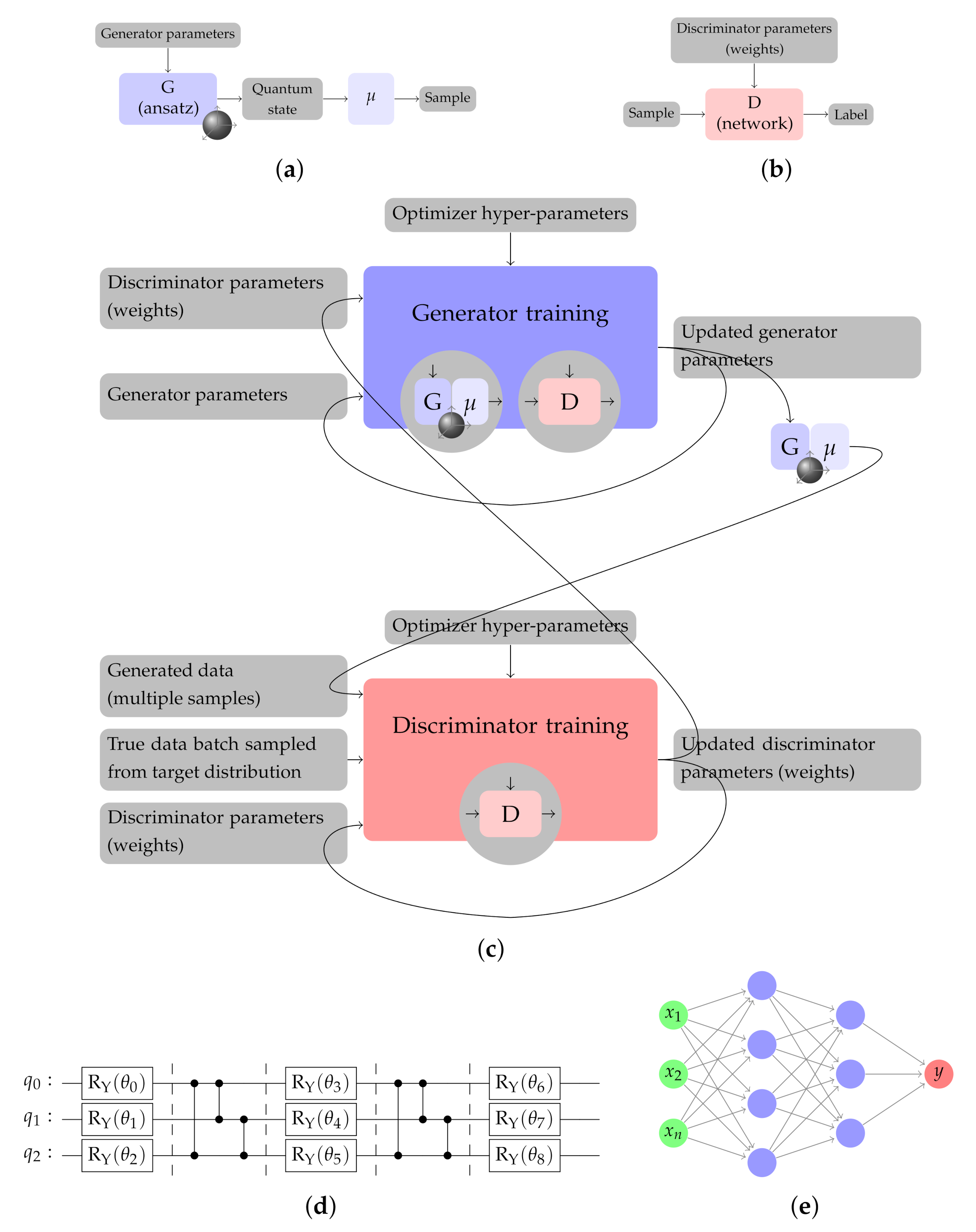
Let us denote the target distribution with , and the approximate distribution achieved by the qGAN with . The generator (Figure 1a) produces a quantum state whose amplitudes are interpreted as the analog encoding of the square root of the approximate probabilities . This way, if the state is measured, i is obtained with probability : in other words, the distribution of circuit measurements equals the approximate distribution. The discriminator (Figure 1b) is a classical neural network that labels a sample as true or fake, according to its ability to discriminate the target data set from the generated data set.
The training of our qGAN (Figure 1c) is performed in epochs. During each epoch, the data sampled from the target distribution are randomly split into batches. For each epoch and batch, fake data are generated by applying the generator with its current parameters and measuring the output state multiple times, then one step of the discriminator training and one step of the generator training occur. The discriminator training algorithms perturbs the discriminator parameters in order to obtain an updated set of parameters that better discriminate true from generated data. The generator training, instead, perturbs the generator parameters, measures multiples samples from the quantum state for each new parameter set, and obtains the labels of such samples by the discriminator so as to identify the generator parameters that most confuse the discriminator. Afterwords, the loop restarts with a new batch. As epochs go by, if the training is convergent, the discriminator learns to identify generated data, while the generator improves its ability to reproduce the reference data. At the end of the training, the generator quantum circuit produces a state distributed approximately like the target distribution.
The choice of the updated parameters for both the discriminator and the generator is made by an optimizer that searches for the descent direction of an objective function. Multiple objective functions can be used in GANs [12]. Following the example of previous qGAN implementations [8], we adopt the so-called non-saturating loss, designed to avoid the effect of insufficient gradient of the generator, which can be observed in the simplest minimax formulation [12].
4.1. Design of the Generative Quantum Circuit Network
In line with the prior art, the ansatz of the generative network is layered, alternating single-qubit rotations with entanglements (see Figure 1d). As far as rotations are concerned, we take gates since they map real amplitudes to real amplitudes. As we want to load probability densities which are real numbers, we can restrict ourselves to explore quantum states with real amplitudes only, instead of spanning a broader, complex-valued manifold. In terms of entanglement gates, following previous literature [8], we use gates. In the entanglement layers we arrange s in a circular fashion: this means applying gates between j-th and -th qubits, where the j-th is the control qubit, for all and also between the -th and 0th.
Given the said choice of the entanglement layer, testing the circuit for qubits only is trivial since and the whole circuit reduces to single-qubit rotations.
Here, the free hyper-parameter for the ansatz is the number k of layers of rotations and entanglements, known as the number of repetitions. A circuit with k repetitions has 1 initial rotation layer, plus k entanglement and rotation layers, resulting in parameters to be trained, which correspond to the rotation angles.
4.2. Design of the Classical Discriminative Deep Neural Network
The discriminative network takes one sample in input at a time, and returns a number between 0 and 1, which aims at indicating how likely the sample is to have been drawn from the generated distribution rather than from the target discretized one.
Suppose the target distribution has d dimensions, then one sample can be represented as a d-tuple , where is a label in and is the number of qubits used to represent the j-th dimension. In previous implementations, labels were fed to the discriminator, which then had d input nodes. In our case, conversely, each individual qubit is an input node such that we end up with a much bigger input layer of nodes, where . Such choice is agnostic to the data structure, as it removes the implicit assumption that the most significant digits in the labels should have a stronger effect on the network. On the other side, it induces a higher cost in terms of training time, since the input layer of the discriminator has more nodes than that adopted in literature. This choice should be reconsidered when the number of qubits grows to validate if the training time remains sustainable.
As a consequence of the aforementioned choice, we treat univariate and multivariate distributions alike. More explicitly, take any integer a, and consider two different distributions, X and Y. The former is a univariate (i.e., ) ranged in , namely . The latter, instead, is a multivariate with dimensions, each ranged in (i.e., ). Additionally, assume that X and Y have the same probabilities, in the following sense: for all , let , where represents the j-th digit of l as a binary string. Under these conditions, the two distributions are trained and loaded in the same manner by our qGAN.
4.3. Optimization of the qGAN Accuracy and Comparison with Benchmarks
To improve the fit of the generated distribution, in addition to the modification of the discriminator design described in Section 4.2, we also fine-tuned the hyper-parameters of the optimizer. Such an objective is achieved through an extensive testing campaign, extensively detailed in Appendix A. The main outcome for qubits is that a high accuracy can be obtained with the Adam AMSGRAD optimizer with a discriminator learning rate of (see Figure A4), and a generator learning rate between and (see again Figure A4). The beta parameters of the optimizers can be chosen to be for both the discriminator and the generator (compare Figure A4 and Figure A5). Under such conditions, the discriminator size—given by the number and of nodes in the two hidden layers—does not influence the result substantially as far as both and are greater or equal to the critical value of 8 (see Figure A2). An appropriate number of shots is (see Figure A6). These results are obtained by means of the test for goodness of fit, as motivated in Section 5.2.
Results of the training with such hyper-parameters are shown in Figure A3, where we calculate two other metrics, namely the Kolmogorov–Smirnov statistic and the relative entropy, for comparison with prior art (we refer to Table I in [8]). For both metrics, lower values mean a better performance. In conditions similar to ours, namely a 3-qubit log-normal target distribution and layers, with random initialization, the previous benchmark was and , with deviations and . By picking instead the best initialization strategy therein proposed, which was the ‘uniform’ initialization in the specific case, the previous paper achieved and , with deviations and . Such results were obtained with a discriminator size of . In contrast, with an even smaller discriminator size of , we can get and , with lower deviations and , giving an improvement of in the KS against the similar case, and of against the best case. We also prove consistency of such a result when modifying the discriminator size (see Figure A3), with an average result of and , and deviations of and .
Appendix A also contains the hyper-parameter tuning for the SPSA optimizer and the case of qubits. For such cases, though, there are no benchmarks in the literature, to the best of our knowledge.
All the simulations were obtained with a lognormal target distribution and with the design of the ansatz described in Section 4.1. Therefore, our results are contextual to such choices. Nonetheless, no previous work showed a specific favorable link between the lognormal distribution and our ansatz, nor is such a link implied by any simple theoretical argument. So, we can expect our result to be representative of the general case.
4.4. Trade-Off between Accuracy and Training Time: The Effect of the Optimizer and of Other Hyper-Parameters
Now let us analyze the trade-off between solution accuracy and training time. We focus our analysis on the simple case of 3 qubits, while we discuss in Section 5.4 that an asymptotic study of the performance needs some key assumptions on the respective scaling of involved variables. Such assumptions require a testing campaign for multiple, high values of n, that is not feasible for the state of the art, given the practical limits of simulators and the scarcity of available computing time on quantum devices.
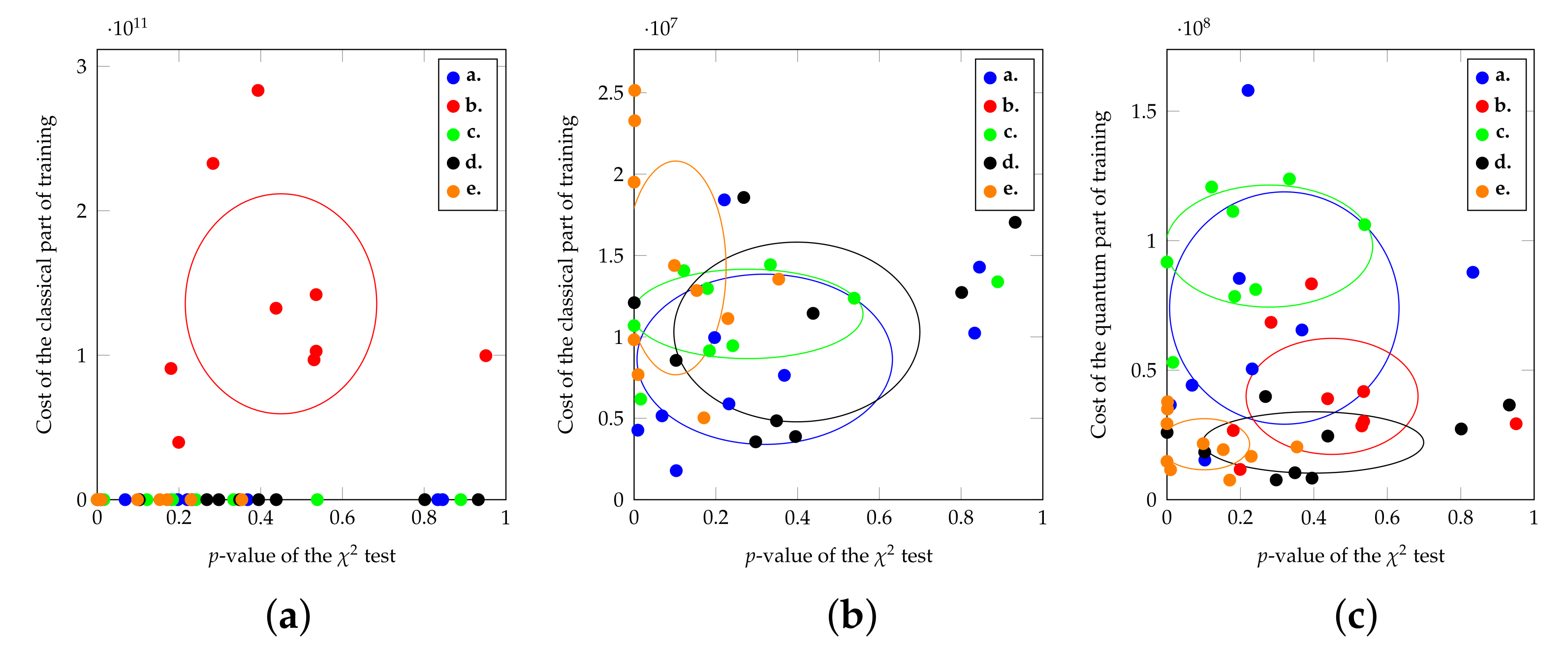
Figure 2 visualizes the trade-off between training complexity on one side, and accuracy on the other side, for a 3-qubit training problem. The former is expressed through a complexity cost function, representing the number of elementary operations performed. It is calculated according to Equations (8) and (9) given in Section 5.4, with some additional simplifications: (a) we discarded the optimizer-specific multiplicative constants, namely and , that express the number of evaluations of the objective function performed in each direction explored by the optimizer in each training step; (b) we discarded the number b of batches in which the training set is split during each training epoch, as we assume it to be fixed, and therefore a multiplicative constant as well; (c) we dropped the quantum training cost of the discriminator from Formula (9) since it never dominates the quantum training cost of the generator . Accuracy, instead, is measured by the p-values of a test for goodness of fit, as discussed in Section 5.2. The values are calculated for five different scenarios, summarized in Table 2 and further detailed in Table A2.
It is clear from the figure that a longer training time in a single run, does not directly imply better accuracy. Indeed, a longer training on a single shot simply means that the optimizer had to explore a wider space before reaching convergence, which may be due only to an unfavorable random initialization.
The figure should be better read under another lens: it is of interest to identify whether a scenario (namely, a set of hyper-parameters) has an effect in terms of the training time and achieved quality in its average run. A trade-off is realized when one dimension improves and the other worsens. Figure 2a shows that the increase in the discriminative network size (case b) implies a significant cost overhead in the classical computation, but no relevant quality improvement, compared to the baseline case a, so a appears certainly preferable to b In Figure 2b,c, we can observe the effect—visible but not dramatically so—of a sub-optimal choice of the learning rate (case c). Again, a is preferable to b. We can also notice that an increase in the number of shots (case d) does not have a major impact on the classical computational cost: in other words, the increased time spent in each epoch is balanced by a reduced number of epochs necessary to achieve convergence. Case d is preferable to a in terms of the quantum training cost.
Finally, we can compare the performance of two optimizers: namely, Adam AMSGRAD, which is a widely used [8] gradient-based technique, and SPSA, which is a gradient-free method. The latter is potentially faster, as it does not need to calculate the complete gradient, thus requiring significantly fewer evaluations of the circuit when the number of ansatz parameters grows (see Section 5.4). Unfortunately, after our testing campaign, we conclude that the faster convergence of SPSA comes at the cost of an accuracy of the solution that is hardly acceptable under our metrics. In Figure 2b,c, we represented through case e the adoption of SPSA in the generator, keeping Adam for the discriminator. We show that the quantum cost of SPSA is lower in case e, compared to a, but the quality of the output is dramatically degraded. Notably, the classical cost increases, as the number of epochs before convergence is higher. We did not include in the Figure the case of SPSA in the discriminator, or SPSA in both the generator and the discriminator, as they achieve even worse accuracy. The interested reader can refer to Appendix A for these additional cases, as well as for a more detailed analysis of all the hyper-parameters.
In conclusion, with the Adam optimizer, the hyper-parameters do not exhibit any trade-off between accuracy and training time, as each hyper-parameter mostly affects one of them. Vice versa, there is a trade-off between Adam and SPSA, in the sense that Adam provides highly accurate results, whilst the latter is faster in terms of quantum training.
4.5. Isolation of the Best Runs
When repeating the training of a qGAN multiple times, one obtains different results, according to the different random initialization of the training process, as detailed in Section 5.2. As expected, the optimization does not always reach the global optimum but gets often stuck in local sub-optima. As a consequence, if we measure the p-value of the test (which is our key measure for goodness of fit; refer again to Section 5.2) after many training processes, we obtain different values.
A key finding of our testing campaign on Adam AMSGRAD for 3 qubits is that there is no continuum in the p-values obtained after training. On the contrary, the best runs concentrate around a p-value of , with some tails as low as , and are well isolated from the other runs, which achieve values below (see Figure A2f, Figure A4f and Figure A5f).
Therefore, in order to achieve a high quality approximation, is it more important to try many initial configurations, rather than training only one very carefully. Indeed, perturbations of the optimal hyper-parameters do not affect results as dramatically as the initial conditions or the choice of the optimizer do (Appendix A).
The phenomenon is the result of an intrinsic characteristic of the training problem, not previously reported, to the best of the authors’ knowledge. Better understanding the reason of such behavior may provide insights for a more effective choice of the initial parameters, or for the early discarding of ill choices. We conducted a preliminary study detailed in Appendix B that suggests that an elbow in the parameters before convergence likely means optimality, while sub-optimal runs have either slow or oscillatory convergence, or residual dynamics after convergence (see Figure A14).
The isolation was observed with clarity under specific conditions: the optimizer Adam AMSGRAD, qubits, the lognormal target distribution, and the ansatz design illustrated in Section 4.1. Our tests on other optimizers and number of qubits do not allow us to either accept nor reject with confidence the generality of the behavior.
5. Methods
The current section collects the methods applied to obtain results. Much of the design follows Ref. [8], so for clarity, we anticipate here the key differences. We define the concept of converging run, which was absent in the previous paper and we mostly resort to the test for assessing the solution quality instead of the Kolmogorov–Smirnov statistic. We test the behavior of the SPSA optimizer in addition to Adam AMSGRAD and we modify the design of the discriminative network, as explained in Section 4.2. Finally, we conduct a broader testing campaign on the hyper-parameters, and study their influence on the converging rate, on the output accuracy, and on the computational cost.
5.1. Testing Conditions
We conduct our tests through the ‘Qiskit’ library [52]. Qiskit allows for the circuits to be run on different device types: (a) the statevector simulator, which can compute the exact state resulting after the circuit application, under perfect conditions, (b) the noiseless simulator, which emulates the circuit behavior in ideal conditions, but applies a number of measurements according to the number of shots provided, thus resulting in an approximate knowledge of the circuit output, (c) the noisy simulators, which apply a noise model whenever gates are executed, and (d) real hardware, typically resorting to the devices provided by IBM in cloud.
Preliminary tests highlight a significant difference in the convergence behavior of the training process, between the results obtained on the statevector simulation compared to the noiseless simulation since the approximation induced by a finite number of measurements gives stronger oscillations to the neural network and forces to consider bigger neighborhoods of the network parameters for the evaluation of gradient to avoid local flatness. Vice versa, the difference between noiseless and noisy simulators is negligible. Such an observation can be explained with the resiliency of neural networks to noise, and with the shallow depth of our circuits. The execution time, nonetheless, is much higher in noisy simulations, due to the need to artificially reproduce noise in the simulator. The execution of extensive testing campaigns of hybrid algorithms on quantum hardware is difficult at the current state of the art due to the long delay required to connect to the backends. Provided such considerations, our training process is carried on the noiseless simulator, which provides the best trade-off in terms of execution time versus result significance, for our purposes, at the time of writing.
We test the training of a univariate lognormal with parameters and , discretized in bins in the domain . The choice of the lognormal is inherited from prior work [8], and it is motivated by its usefulness in the financial domain. A univariate distribution allows for direct comparison with previous literature, and at the same time, does not imply a loss in generality since our design of the discriminator makes the training of the univariate fully equivalent to that of a multivariate, as explained in Section 4.2.
The training set is made of 20,000 samples, which decreases after binning, since tails are trimmed. This way, we obtain around 17,200 samples, which is the number S of samples that we use to feed the training.
Before applying the ansatz, the circuit is prepared to the initial state . In each epoch, following once again the approach of Ref. [8], the training data set is shuffled and split into batches. We take the batch size of 2000, namely around one tenth of the data set size.
Each quantum circuit is evaluated on s shots, as indicated in Table A1, in order to properly account for the statistical nature of measurement.
5.2. Run Evaluation
In our testing campaign, described in Appendix A, we execute many different simulations. Every test is repeated 10 times to ensure robustness of the outcomes. Therefore, the 10 simulations differ for the random initialization of the generator parameters of the discriminator parameters and of all randomized behaviors in the optimizers (seed, batching, etc.). The metrics of each run are calculated individually and then aggregated among the 10 runs, giving rise to an average-case result and a best-case result.
Indeed, let us emphasize that independent runs obtained with the same hyper-parameters are far from being uniform in terms of training results, as shown in Appendix A. Nonetheless, an appropriate choice of the hyper-parameters increases the probability of obtaining better outcomes.
In order to assess a single run, we have to address two key aspects: (a) We must ensure that the training process comes to convergence before reaching the end of the available training epochs, and this means that we need a formal definition for training convergence. (b) We also need to measure the quality of the output and compare it to a fixed threshold, which is our acceptable precision.
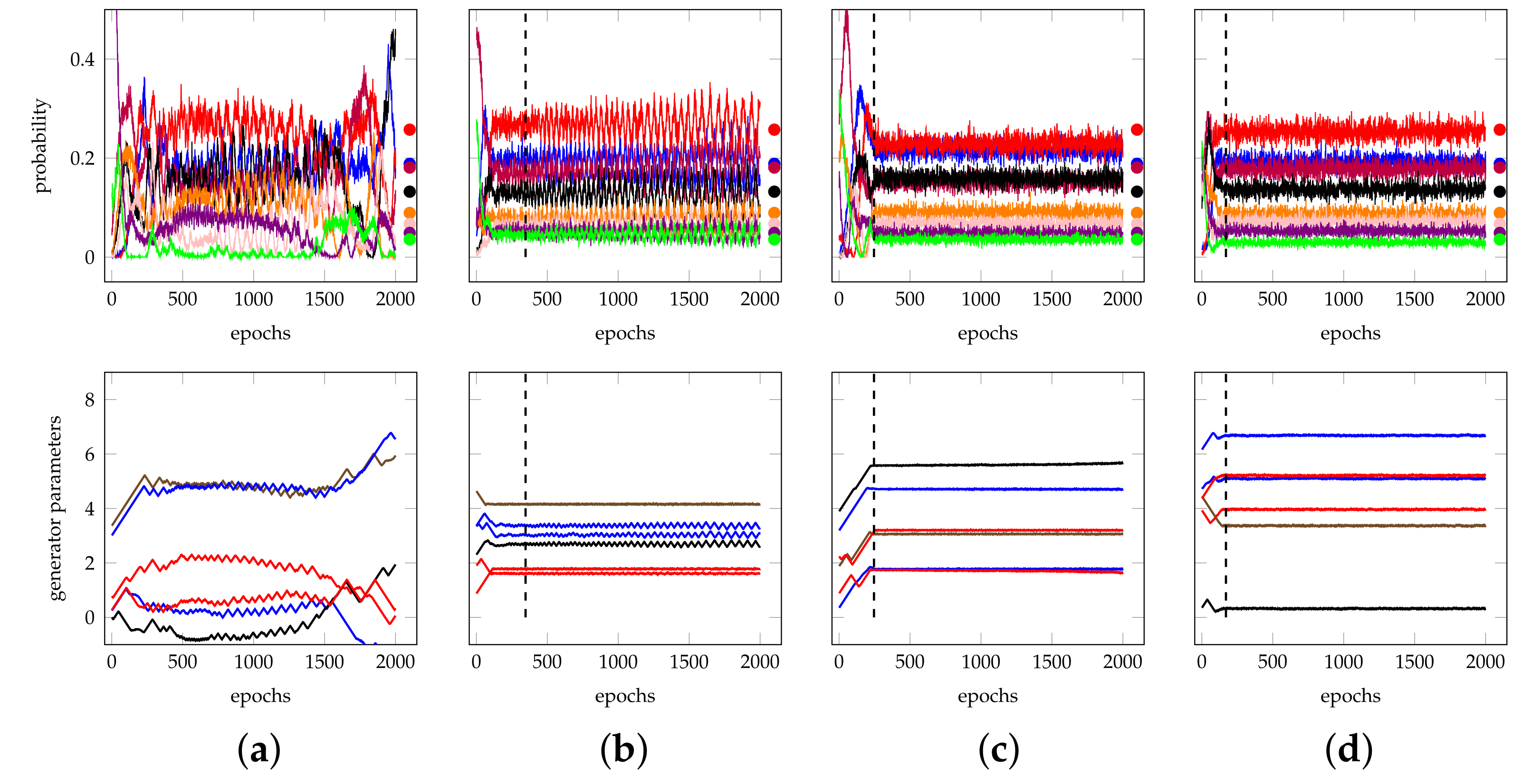
Let us start by discussing the convergence. Due to the randomness of the input data, it is expected and a priori acceptable to have oscillations in the solution. What we need to check is that oscillations happen around a target value, and there is no substantial movement of any parameter in a given direction (see Figure 3b–d). A run converges to a local solution in j epochs, if all the generator parameters are substantially stable for a given number m of epochs after j. Based on that, we can provide the definition of convergence: let M be the total number of epochs in our test, then for each parameter and for each candidate epoch j starting from 0 and increasing, we make a linear regression along the subsequent epochs and check whether the absolute value of the line slope is controlled by of the generator learning rate. If so, we find j (when the learning rate is variable, we check the slope is controlled by , which is consistent with the baseline learning rate of ). Notice that we deliberately neglect to verify the convergence of the discriminator parameters, because our core objective is obtaining the generator parameters only, as they contain the representation of the approximated distribution. In other words, we accept an under-determined discriminator, as long as it is able to drive the generator to convergence.
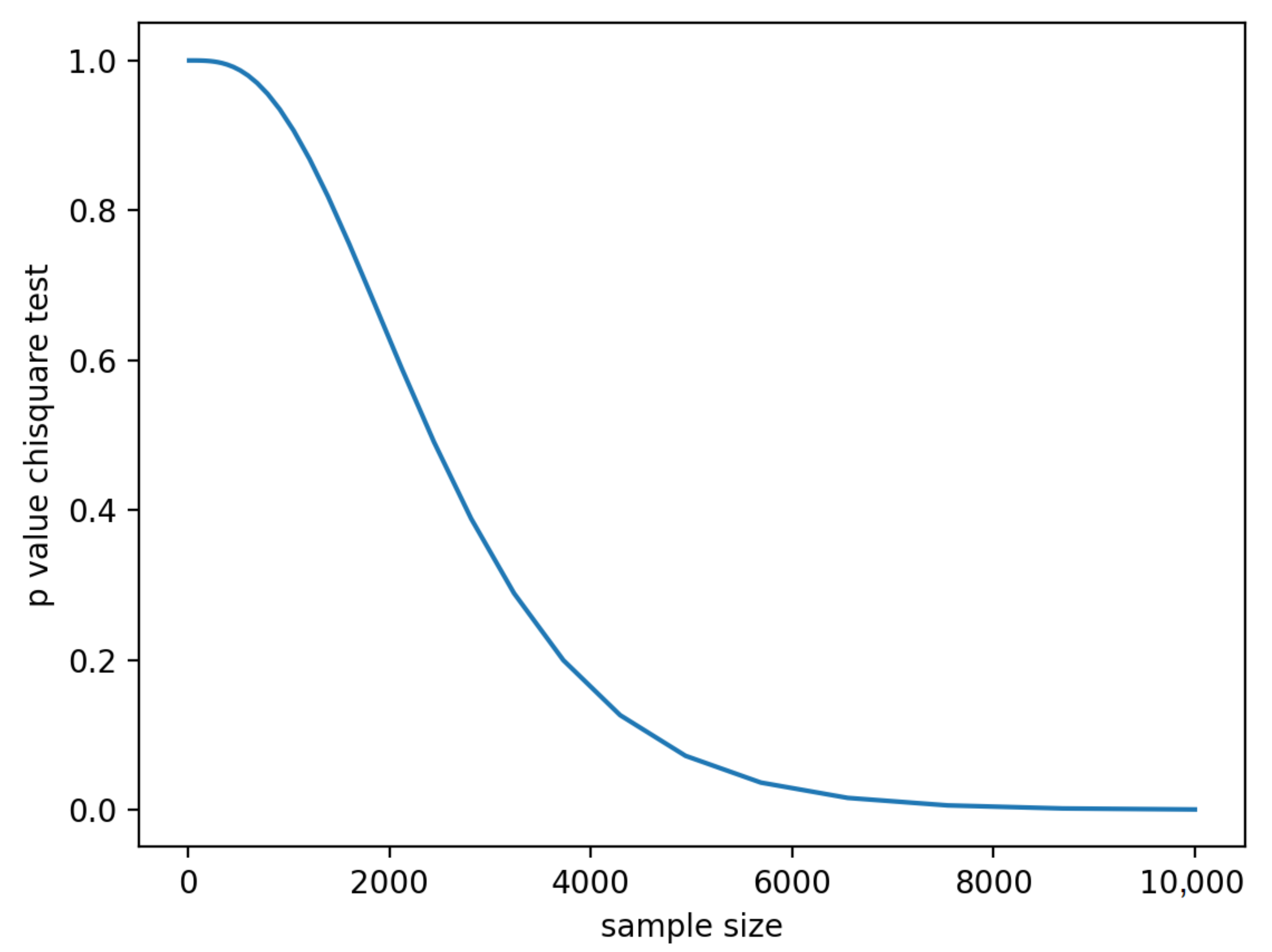
The second topic is the quality of the solution: indeed, a convergent run may still find a bad approximation of the target distribution (see Figure 3c), either due to the optimizer finding a sub-optimal solution, or due to the ansatz not reaching any point close enough to the target. As said in Section 5.1, the training process is performed on a noiseless simulator. Nonetheless, after completing the training, we measure the quality of the solution by evaluating the circuit with the trained parameters on a statevector simulator such that we remove the effect of a finite number of measurements. The topic of selecting evaluation metrics for GANs is open and broadly discussed [12]. For our purposes, we evaluate the quality of the solution by performing a test, for goodness of fit. We choose the test instead of the Kolmogorov–Smirnov test used in previous literature [8], as it is more representative for discrete variables with a small number of domain buckets, and more easily exportable to multivariates. We also run the Kolmogorov–Smirnov test for comparison with prior work in Section 4. Since we are looking for approximate solutions, the target distribution is not exactly the trained distribution, and if a test is run with a huge sample size, one will certainly discriminate them and reject the null hypothesis. On the contrary, being able to well approximate a distribution means making it hard to discriminate the generated distribution from the target one, when looking at a relatively small, fixed number s of samples. Figure 4 shows that the test gets easily confused when the number of samples is small, and improves at discriminating when the sample size grows. For the experiments in Section 4, we calculated the p-value based on a 2-sample test where we used the full sample S of around 17,200 values for the target distribution and a size for the generated distribution by recurring to the ’scipy´ implementation [53].
5.3. Objective Function and Optimizers
We study the training process with two different optimizers, the Adam AMSGRAD and the SPSA. The former is used as a benchmark, following Ref. [8], while the latter is particularly interesting, as it is a gradient-free optimizer.
Gradient-free optimizers are becoming popular in quantum computing [54,55]. On one side, they promise to mitigate the barren plateau effect [56,57,58,59], even if their actual ability to overcome such a problem is still debated [60]. Moreover, they require fewer evaluations of the objective function when the dimension is high (see Section 5.4), suggesting a potential benefit in terms of training times (discussed in Section 4.4 for the qGAN problem).
More specifically, we resort to the Adam AMSGRAD optimizer provided by Qiskit for the discriminator, while we use its implementation in Pytorch ([61]), which is linked into Qiskit itself, for the discriminator. As far as SPSA is concerned, we exploit the Qiskit version.
The most relevant hyper-parameters of Adam AMSGRAD that affect performance are the learning rate, and , while those of SPSA are the learning rate and the perturbation factor.
5.4. Estimating Complexity
When measuring computational complexity, two different processes have to be considered: the training process, which is performed once for a given distribution, and the process of loading data into a quantum computer through previously trained parameters, which can be performed multiple times for the same distribution, depending on the subsequent use of the loaded data. In this subsection, we derive an estimate for both the loading and the training costs.
First of all, let us call the cost of evaluating the ansatz, namely, running the ansatz circuit once with the given parameters. We measure the computational complexity of quantum circuits in terms of circuit depth such that we obtain
where n is the number of qubits, and k the number of repetitions, defined in Section 4.1. The superscript q indicates that the cost is due to quantum operations.
The complexity of loading approximate data into the quantum computer with a qGAN is, by definition,
The training complexity is the number of operations required to obtain the approximately optimal generator parameters. The training process involves both classical and quantum computations. Indeed, the basic building blocks of the process are the execution of the ansatz on the quantum side, whose complexity equals and the evaluation of the discriminative network on the classical side at a cost which is essentially given by amount of matrix–vector multiplications, namely,
where and are the number of nodes in the hidden layers, as usual.
During each epoch, and for each batch, a training step of the generator and a training step of the discriminator are performed. Indeed, the generator and discriminator parameters are updated by the optimizer, according to the descent direction.
Each generator training step requires the quantum circuit to be evaluated multiple times, depending on the optimizer. Ref. [55] shows that the number of evaluations is constant for SPSA and scales linearly with the number of parameters for gradient-based methods, which is ,
where the constant is a characteristic of the optimizer used by the generator, and s is the number of shots of the quantum circuit. For each generator training step, the discriminator must be evaluated too, giving rise to a classical cost
During the discriminator training, instead, the generator is evaluated just once during each training step, independently, on the number of evaluations of the discriminator such that the the quantum cost is simply
Therefore, the complexity is essentially that of a usual classical training step for a feed-forward network with parameters, namely,
Therefore, by multiplying by the number of steps, which is the number b of batches times the number j of epochs to reach convergence, we obtain that the total training cost is essentially
Equations (2), (8), and (9) fully describe the loading and training complexity through qGANs. An asymptotic study of such quantities would require assumptions on the scaling of k, , , and j as functions of n, as well as the identification of the bottleneck, either in the classical or in the quantum processing. Unfortunately we cannot infer similar information after our study, as we necessarily focused on small values of n due to technological constraints.
6. Conclusions
To conclude, we improved the state-of-the-art accuracy of approximate distributions obtained after the qGAN training by means of a fine tuning of the hyper-parameters, as well as by adjusting the discriminator network. We discussed the choice of two different optimizers, showing that SPSA achieves faster convergence at the cost of a loss in accuracy, which we consider insufficient according to our metrics, as the p-values obtained for 3 qubits are always below 0.5 when SPSA is applied in the generator and below 0.001 when it is applied to the discriminator, while Adam achieves values over 0.95. The increase in the number of qubits implies a significant decrease in the accuracy measured by the test for goodness of fit. The random initial parameters for training strongly affect the ability to reach an optimal rather than a sub-optimal accuracy. Indeed, attempting the training multiple times with different initial parameters is a major strategy to reach satisfactory outcomes, and is even more important than fine tuning the hyper-parameters. We also highlighted a peculiar phenomenon of a net separation of the runs achieving optimal accuracy, whose p-values are clustered far away from sub-optimal runs, and provided a first qualitative analysis, suggesting that an elbow in parameters before convergence could be an indicator of an optimal run, while slow, oscillatory behaviors are likely symptoms of sub-optimal runs. Our improved results were achieved by means of a testing campaign, as well as a slight redesign of the discriminative network. The modification of the discriminator also allowed us to treat univariate and multivariate distributions similarly, thus giving value to our study in the context of multivariates.
Given the relatively small size of the problem we could test, we necessarily focused on memorization (the ability to fully replicate a data set), rather than generalization (the ability to produce data that resemble those in the training data set, producing realistic but unseen data). It is known for classical GANs that memorization is harder than generalization and generally discouraged [12,62].
As a consequence, natural research paths for the future are the validation of the results with a higher number of qubits and a scaling study.
Author Contributions
Conceptualization, G.A. and E.P.; software, G.A.; validation, E.P.; writing—original draft preparation, G.A.; writing—review and editing, E.P.; supervision, E.P. All authors have read and agreed to the published version of the manuscript.
Funding
The access to the IBM Quantum Research Program was granted by IBM.
Institutional Review Board Statement
Not applicable.
Informed Consent Statement
Not applicable.
Data Availability Statement
The data that support the findings of this study are available from the corresponding author upon reasonable request.
Acknowledgments
The authors are thankful for the access to the IBM Quantum Researchers Program. G.A. is grateful to Christa Zoufal for the profitable conversations.
Conflicts of Interest
The authors declare no conflict of interest.
Appendix A. Tuning a qGAN
When trying to implement a qGAN for a specific application, one needs to identify the ‘optimal’ setting so that the trained circuit closely approximates the target distribution. Here, optimality is defined at least by two conflicting metrics: training time and approximation quality. On one hand, the training should be as fast as possible, meaning that a high probability of convergence is targeted, together with a low number of convergence epochs j. On the other hand, the generated distribution should resemble the original one as closely as possible, so we want a high p-value for accepting the trained circuit. The testing policies and metrics are defined more precisely in Section 5 and particularly in Section 5.2.
Appendix A.1. Summary of Choices and Tunable Degrees of Freedom
The generator and discriminator size are levers that affect the training process quality. The number n of qubits impacts on the input size of the discriminator and the output of the generator. As discussed in Section 4.1, the generator is a quantum circuit composed by two types of layers (see Figure 1d). In a rotation layer, single-qubit rotations with free parameters are applied to all qubits. In an entanglement layer, selected qubits are coupled through entangling gates. Rotation layers and entanglement layers follow one another multiple times, so that the generator size is driven by the number k of repetitions. The discriminator instead is a classical neural network, with two hidden layers (see Section 4.2). Its size depends on the number of nodes and in the hidden layers.
As a consequence, in order to tune the setting of a qGAN for a given target data set, one wants to study the optimal j, k, and by varying n. As well as in classical machine learning, the training of a qGAN requires the execution of a training algorithm, which is a classical optimizer, in line with the state of the art [46]. This means that the results are strongly affected by the choice of the optimizer, both in terms of quality and time. Therefore, we must care about the optimizer used and its main hyper-parameters: specifically, the learning rates and betas for the Adam AMSGRAD optimizer, and the learning rate and perturbation for the SPSA optimizer, respectively. Lastly, given the probabilistic nature of quantum measurements, the number of shots s (that is, the number of executions of the quantum circuit) affects the result, as well. Refer to Section 5.3 for more details.
Appendix A.2. The Testing Campaign
The tuning of the qGAN is performed through a testing campaign, articulated in different test sets. Each test set is characterized by some fixed settings and some free hyper-parameters: for instance, test set A performs a sensitivity analysis of the generator and discriminator learning rates for the 3 qubit case, while keeping fixed the optimizers and the network size, as well as the number of maximum allowed epochs and the number of shots. Each test set, then, is composed of multiple test cases: in the example of test set A, a specific test case has and . Finally, each test case is repeated 10 times, so that the 10 runs differ by various choices of the random seed, affecting the starting initialization of the network parameters, the random behavior of the optimizers and the randomness of simulated quantum measurements.
The list of the main test sets is contained in Table A1 and commented in the remainder of the section.

Table A1.
The enumeration of the most relevant tests. Every test set provides a sensitivity analysis over some parameters, marked with a star (*) in the table.
Table A1.
The enumeration of the most relevant tests. Every test set provides a sensitivity analysis over some parameters, marked with a star (*) in the table.
| Test Set | n | k | Generator Optimizer | Discriminator Optimizer | Max Epochs | Shots | ||
|---|---|---|---|---|---|---|---|---|
| A | 3 | 1 | 8 | 16 | Adam, lr = *, = 0.7, = 0.99 | Adam, lr = *, = 0.7, = 0.99 | 2000 | 2000 |
| B | 3 | 1 | * | * | Adam, lr = , = 0.7, = 0.99 | Adam, lr = , = 0.7, = 0.99 | 2000 | 2000 |
| C | 3 | 1 | * | * | Adam, lr = , = 0.7, = 0.99 | Adam, lr = , = 0.7, = 0.99 | 2000 | 2000 |
| D | 3 | 1 | * | * | Adam, lr = , = 0.9, = 0.99 | Adam, lr = , = 0.9, = 0.99 | 2000 | 2000 |
| E | 3 | 1 | 8 | 8 | Adam, lr = , = 0.7, = 0.99 | Adam, lr = , = 0.7, = 0.99 | 2000 | * |
| F | 3 | 1 | 8 | 8 | SPSA, lr = *, perturb = * | Adam, lr = , = 0.7, = 0.99 | 10000 | 2000 |
| G | 3 | 1 | 8 | 8 | SPSA, lr = , perturb = | Adam, lr = , = 0.7, = 0.99 | 10,000 | * |
| H | 3 | 1 | 8 | 8 | Adam, lr = , = 0.7, = 0.99 | SPSA, lr = *, perturb = * | 10,000 | 2000 |
| I | 3 | 1 | 8 | 8 | Adam, lr = , = 0.7, = 0.99 | SPSA, lr = , perturb = | 10,000 | * |
| J | 4 | 1 | * | * | Adam, lr = , = 0.7, = 0.99 | Adam, lr = , = 0.7, = 0.99 | 2000 | 2000 |
| K | 4 | 1 | 32 | 16 | Adam, lr = *, = 0.7, = 0.99 | Adam, lr = *, = 0.7, = 0.99 | 2000 | 2000 |
| L | 4 | 1 | 32 | 16 | Adam, lr = , = 0.7, = 0.99 | Adam, lr = , = 0.7, = 0.99 | 2000 | * |
Table A2.
Test cases used in Section 4.4 are selected from tests in Table A1.
Table A2.
Test cases used in Section 4.4 are selected from tests in Table A1.
| Case | Originating Test Set |
|---|---|
| a. Baseline | B with |
| b. Big discriminator size | B with |
| c. Low generator learning rate | C with |
| d. Many shots | E with shots = 8000 |
| e. SPSA in generator | F with lr = and ratio = |
Table A3.
Each run used in Section 5.2 is selected from the 10 runs in the specified test case of Table A1.
Table A3.
Each run used in Section 5.2 is selected from the 10 runs in the specified test case of Table A1.
| Run | Originating Test Set |
|---|---|
| (a) Divergent | B with |
| (b) Oscillatory | B with |
| (c) Poor solution quality | B with |
| (d) Good solution quality | B with |
Let us start with the case of qubits and, specifically, with the Adam optimizer. Figure A1 shows a fine tuning of the learning rates for fixed , showing that a discriminator learning rate as low as provides very unlikely convergence. Compared to the other scenarios, a discriminator learning rate of provides better results in terms of the p-value. Then, we choose the generator learning rate: in this case, both and are good options, with the latter being more dispersed around the mean.
Consequently, in the test sets B (Figure A2) and C (Figure A4), we focus respectively on those values of learning rates, and we try to observe consistency when changing and . The outcome is that both and are confirmed to be good values for the generator learning rate, with the former being more prone to speed and the second to quality, as one expects. A small network size ( or ) provides much lower convergence probabilities, and this effect is more visible with than . Interestingly though, beyond the critical value of , further increasing the size of the network slightly reduces the convergence epochs, but does not substantially improve on the result quality.
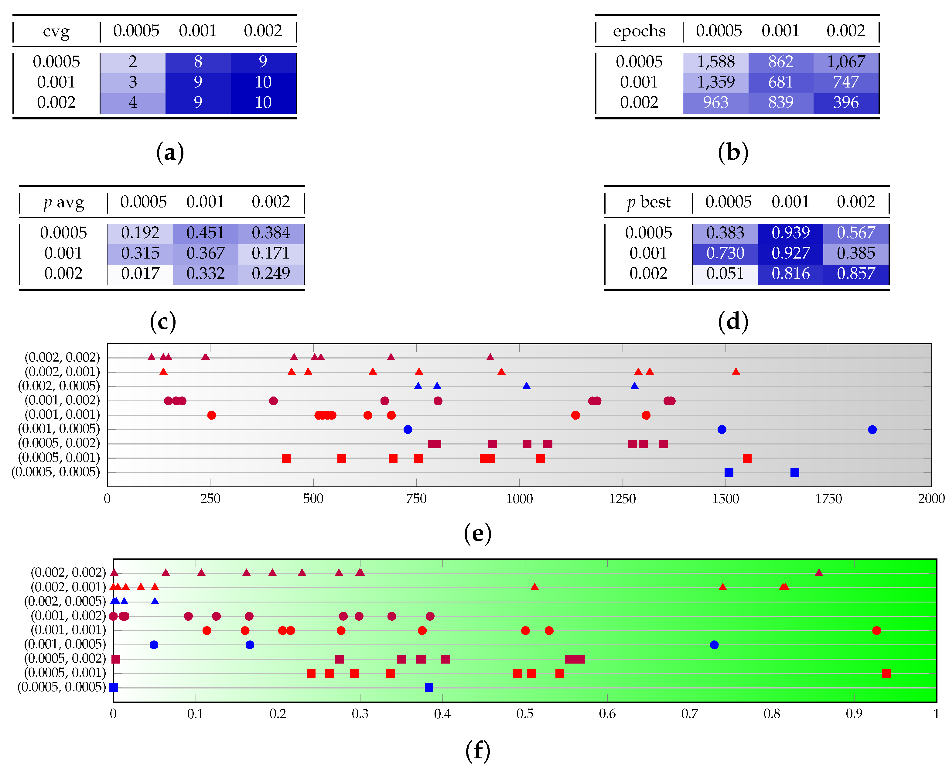
Figure A1.
Test set A provides a sensitivity analysis on the learning rates for Adam. (a–d) The rows represent the generator learning rate, and the columns represent the discriminator learning rate. (e,f) The couples on the vertical axis are . The marker shapes represent and marker colors represent . (a) Converging runs, out of 10. (b) Number of epochs before convergence, on average. (c) p-value for the test once convergence is reached (average over converging runs). (d) p-value for the test once convergence is reached (best run). (e) Visual representation of the epochs before convergence. (f) Visual representation of the p-value.

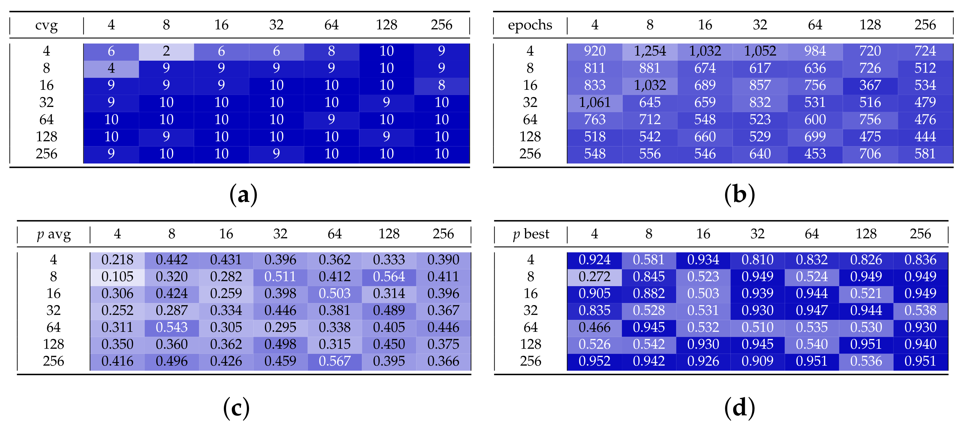
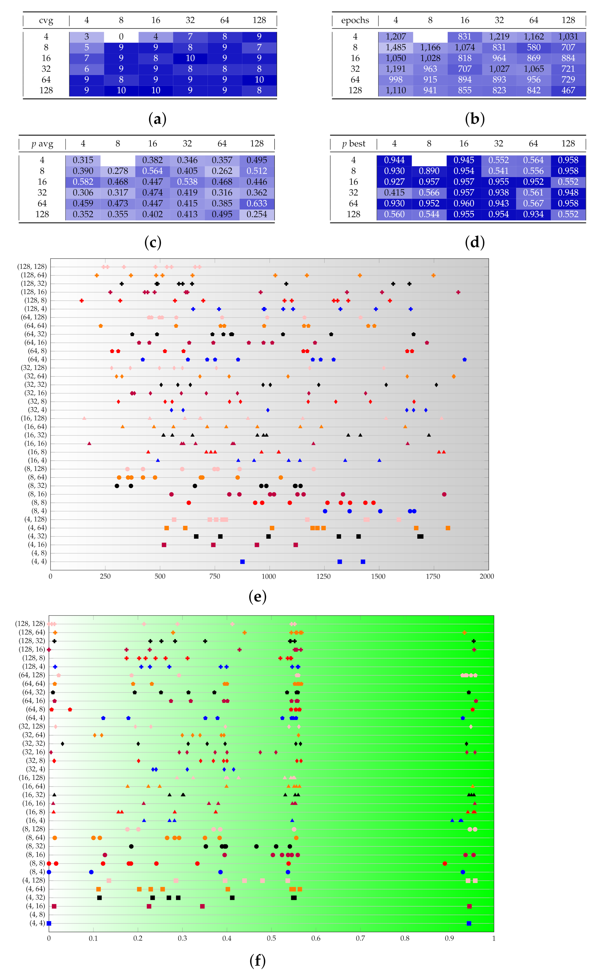
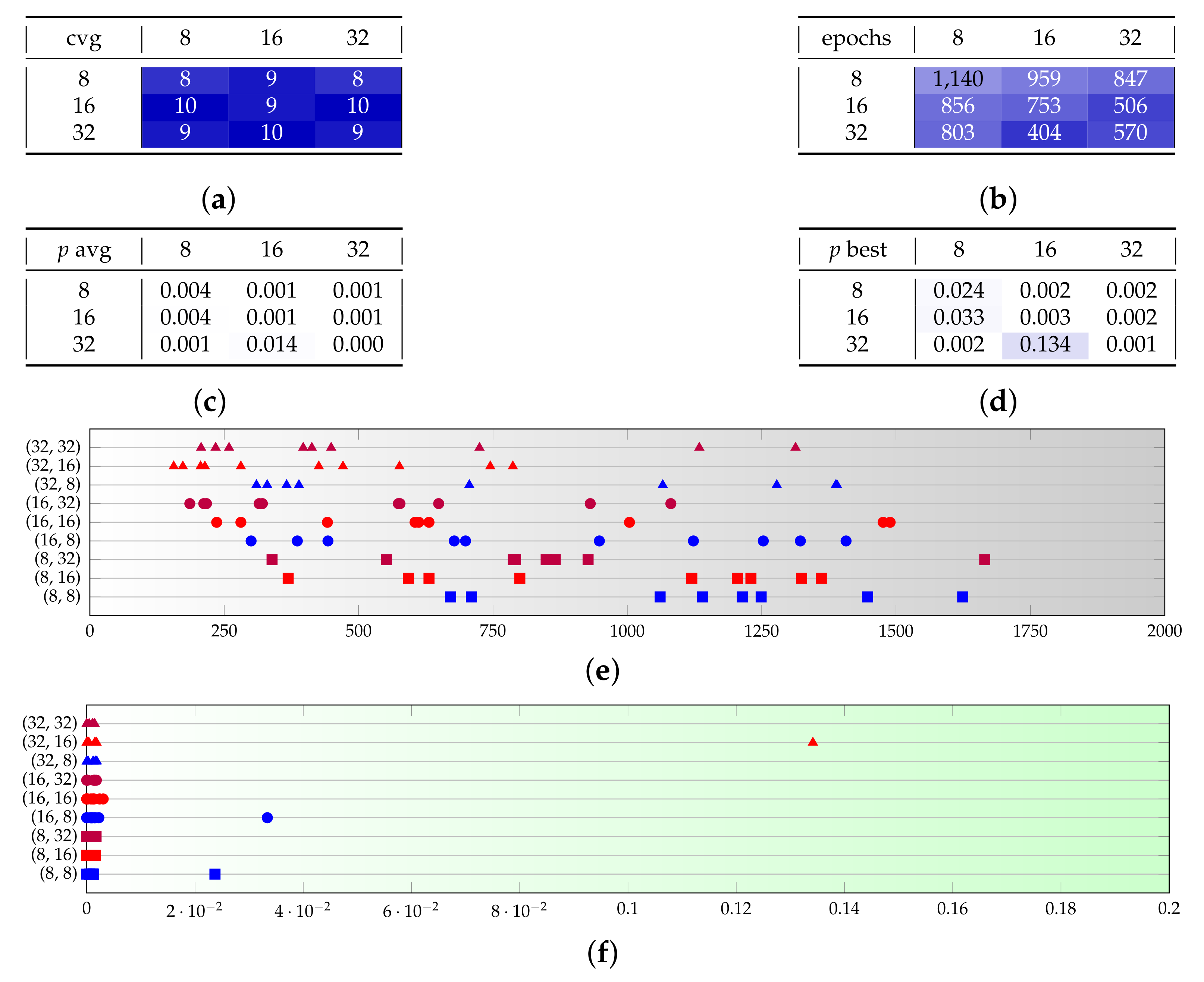
Figure A2.
Test set B provides a sensitivity analysis on the discriminator size. (a–d) The rows represent and the columns . (e,f) The couples on the vertical axis are . Marker shapes represent and marker colors represent . (a) Converging runs, out of 10. (b) Number of epochs before convergence, on average. (c) p-value for the test once convergence is reached (average over converging runs). (d) p-value for the test once convergence is reached (best run). (e) Visual representation of the epochs before convergence. (f) Visual representation of the p-value.


Another very notable remark arises by looking at the distribution of the p-values. Most runs fall in the area of , but there is a significant number of spikes well isolated in the interval . This means that, depending on the randomly initialized conditions, the optimizer may or may not get close to a global optimum. The number of good spikes is not clearly related to the network size, according to our findings. As a consequence, with this problem dimension, it is more relevant to run multiple independent training runs, rather than spending resources in each run.
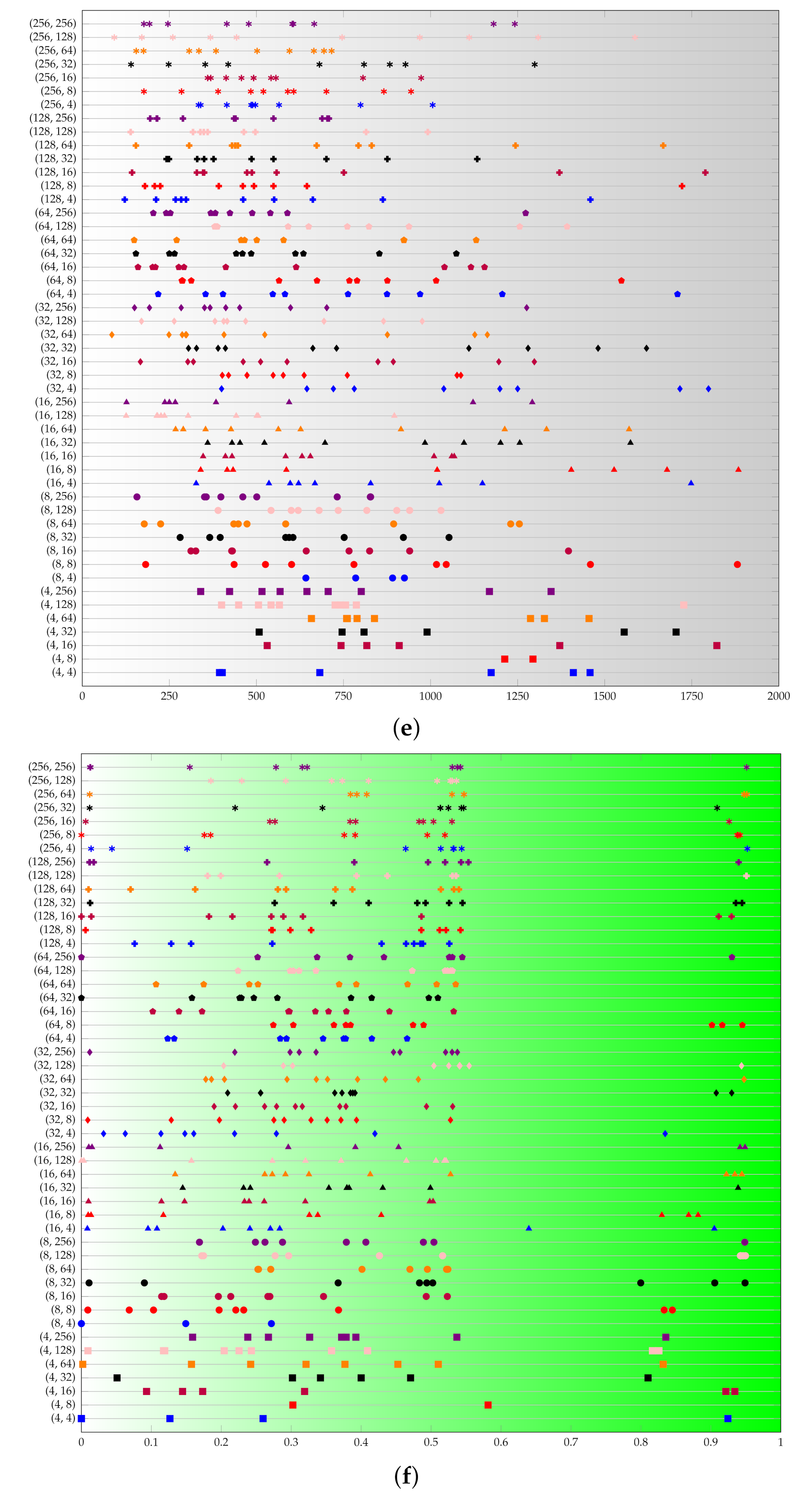
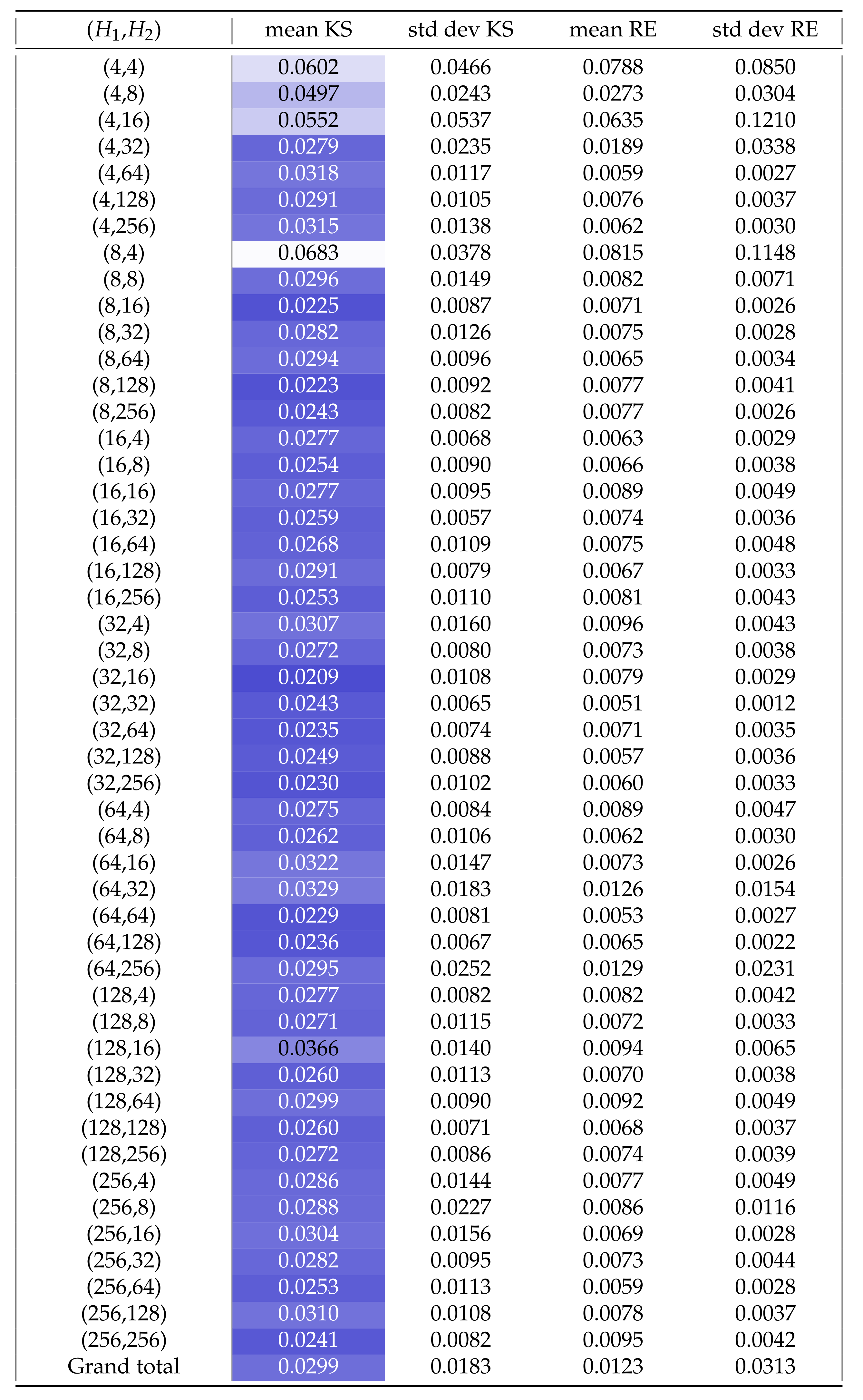
Figure A3.
The values of the Kolmogorov–Smirinov statistic and the relative entropy at the end of the training, from test set B. For both metrics, the lower the better. Notice that we included in the sample also non-convergent runs.
Figure A3.
The values of the Kolmogorov–Smirinov statistic and the relative entropy at the end of the training, from test set B. For both metrics, the lower the better. Notice that we included in the sample also non-convergent runs.

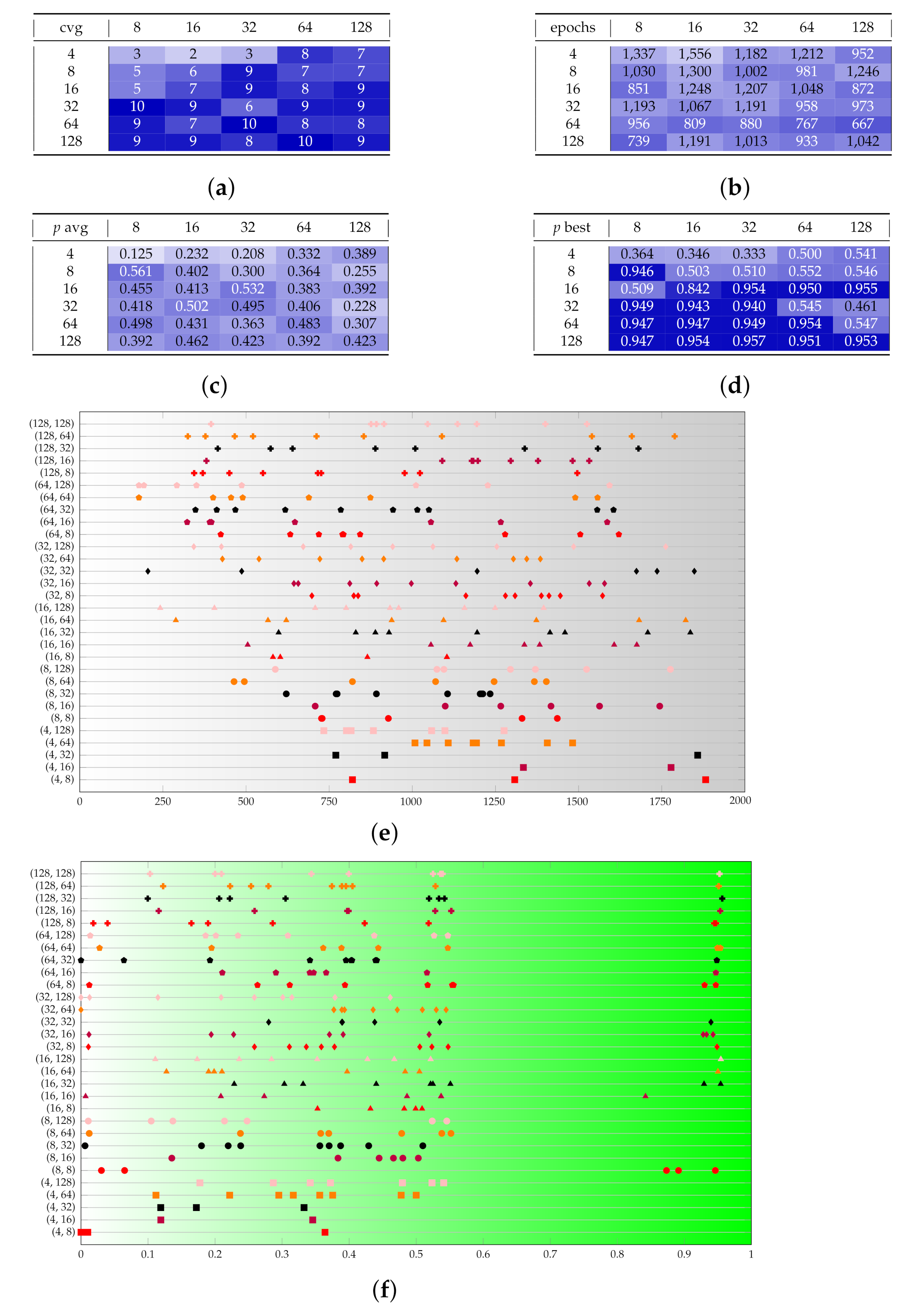
Figure A4.
Test set C provides a sensitivity analysis on the discriminator size. (a–d) The rows represent and the columns . (e,f) The couples on the vertical axis are . Marker shapes represent and marker colors represent . (a) Converging runs, out of 10. (b) Number of epochs before convergence, on average. (c) p-value for the test once convergence is reached (average over converging runs). (d) p-value for the test once convergence is reached (best run). (e) Visual representation of the epochs before convergence. (f) Visual representation of the p-value.

Test set D (in Figure A5) is derived from C by modifying the beta parameters. The new setting does not provide dramatically different outcomes and, compared to the previous one, it shows a preference for scenarios with high and low .
Figure A5.
Test set D provides a sensitivity analysis on the discriminator size. (a–d) The rows represent and the columns . (e,f) The couples on the vertical axis are . The marker shapes represent and marker colors represent . (a) Converging runs, out of 10. (b) Number of epochs before convergence, on average. (c) p-value for the test once convergence is reached (average over converging runs). (d) p-value for the test once convergence is reached (best run). (e) Visual representation of the epochs before convergence. (f) Visual representation of the p-value.

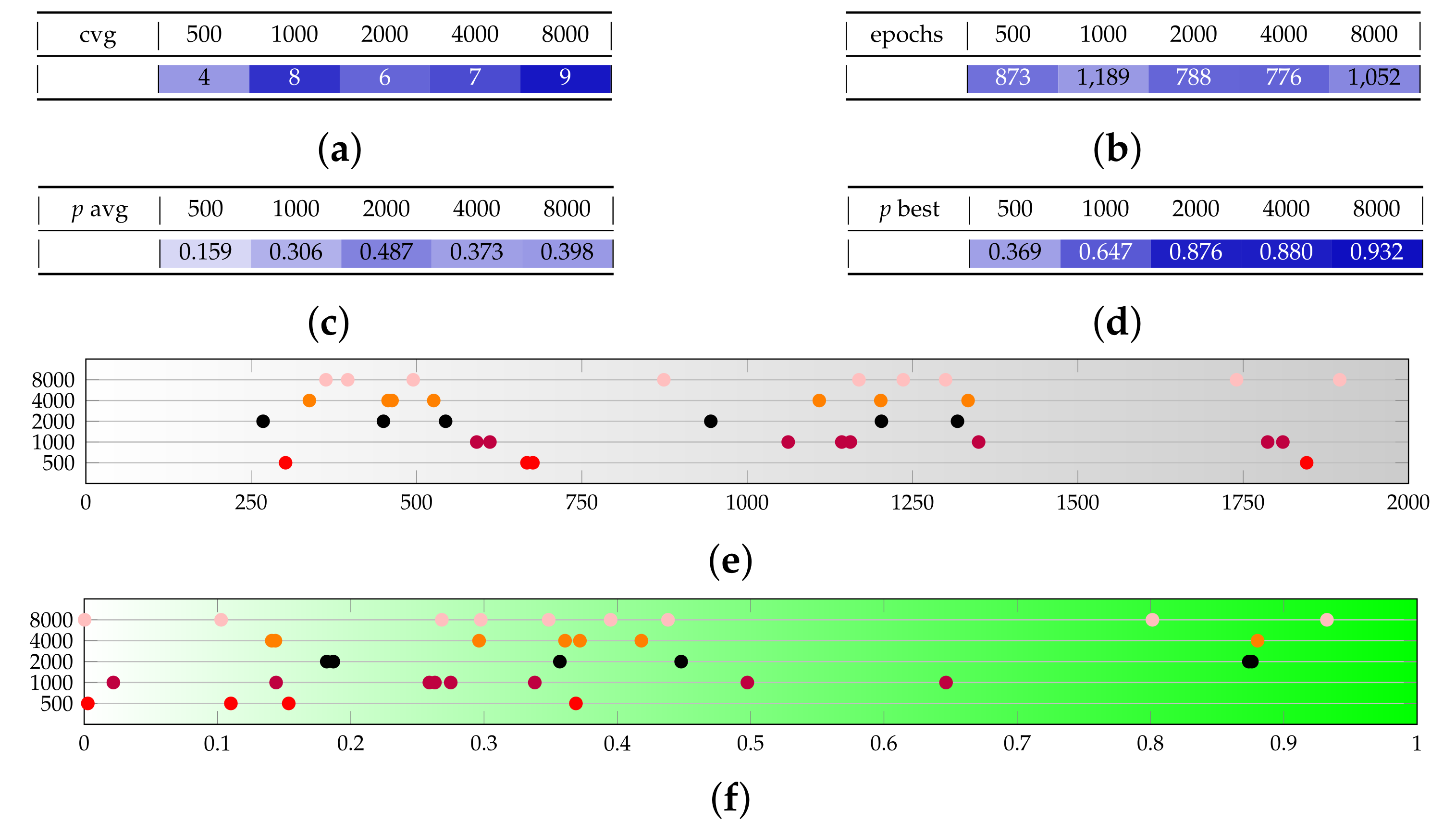
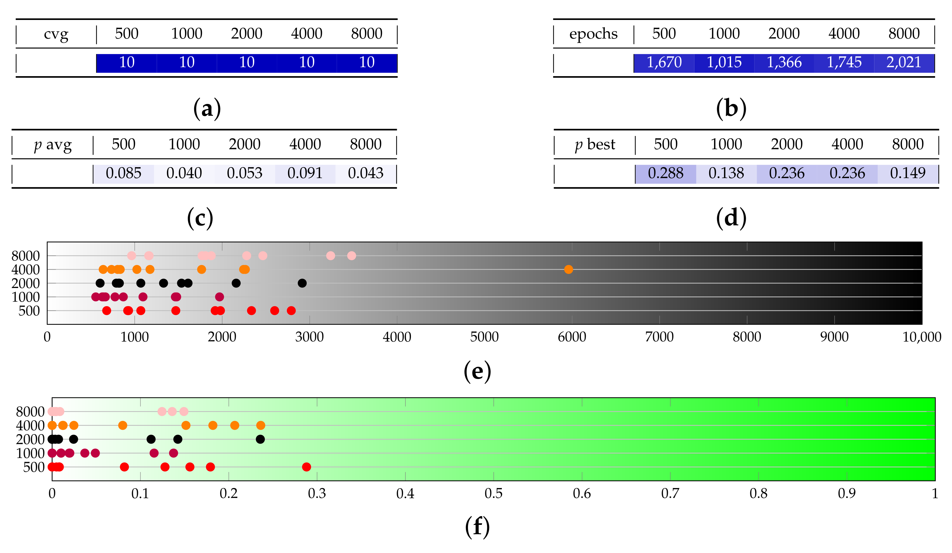
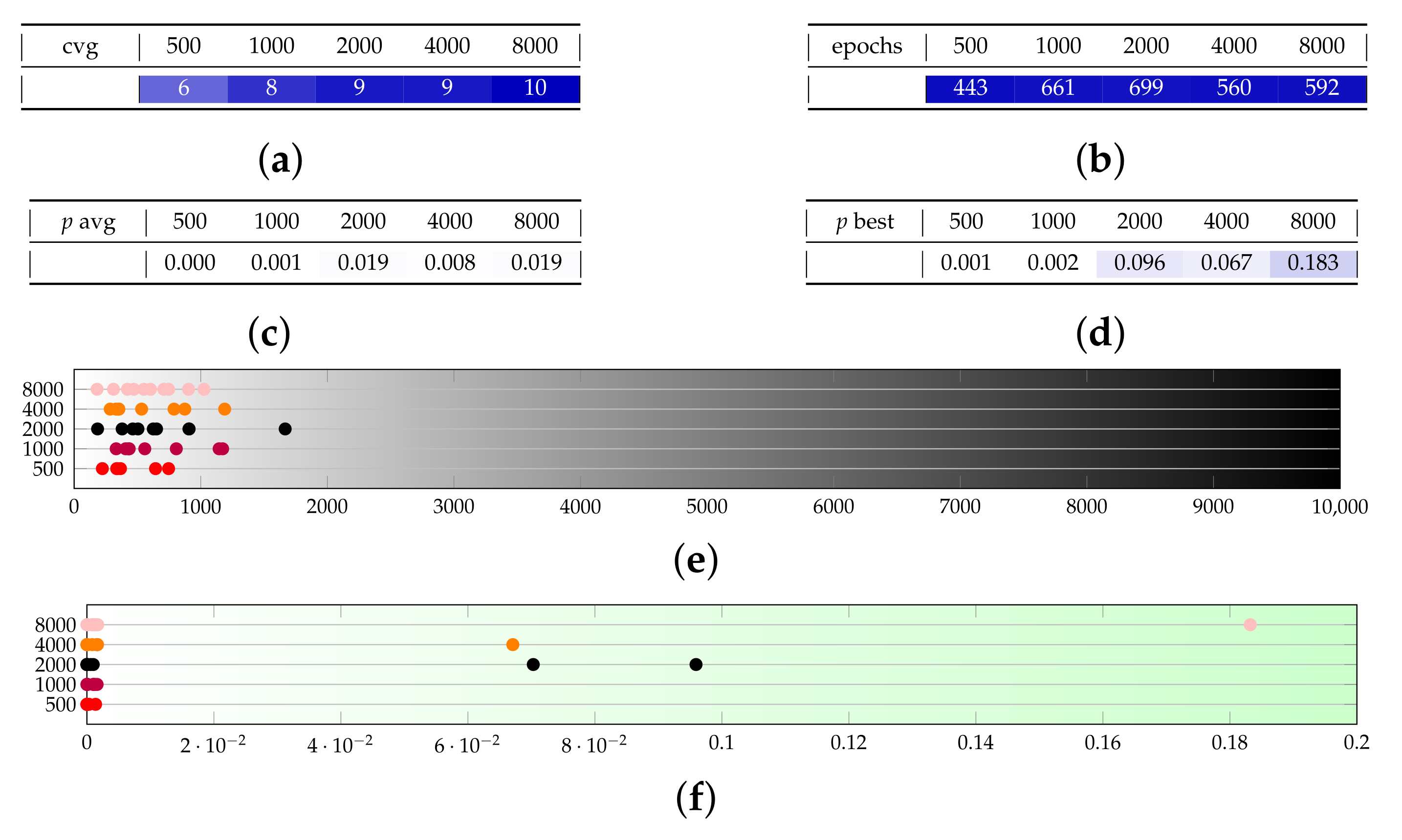
The last parameter we test is the number of shots, that is, the number of times the generator circuit is executed and measured at each evaluation of the generator (that happens multiple times for each epoch). Test set E (in Figure A6) highlights that the effect on the number of converging runs and convergence epochs is negligible, while the spikes of high p-values appear to increase weakly with the number of epochs.
Figure A6.
Test set E provides a sensitivity analysis on the number of shots s. (a) Converging runs, out of 10. (b) Number of epochs before convergence, on average. (c) p-value for the test once convergence is reached (average over converging runs). (d) p-value for the test once convergence is reached (best run). (e) Visual representation of the epochs before convergence. (f) Visual representation of the p-value.

As a conclusion on tests for Adam with , we can say that a good performance is a p-value above for the average run, and that for , we can often expect to find a best run of . Let us remark that we achieved significantly improved performance with respect to the state of the art as an effect of a different definition of the generator network (refer to Section 4.1) and of a better fine-tuning of the optimization hyper-parameters. Indeed, as a benchmark, we calculated the Kolmogorov–Smirnov statistic and the relative entropy of the different runs in Figure A3, for comparison with Table I of Ref. [8], providing a value of mean KS equal to , variance , mean RE and variance . Our average performance is as low as of the benchmark in terms of KS, considering all runs in Figure A3, and for the best choice . It comes at a slightly higher cost in terms of training time since our first layer of the generator is bigger than those adopted in previous literature.
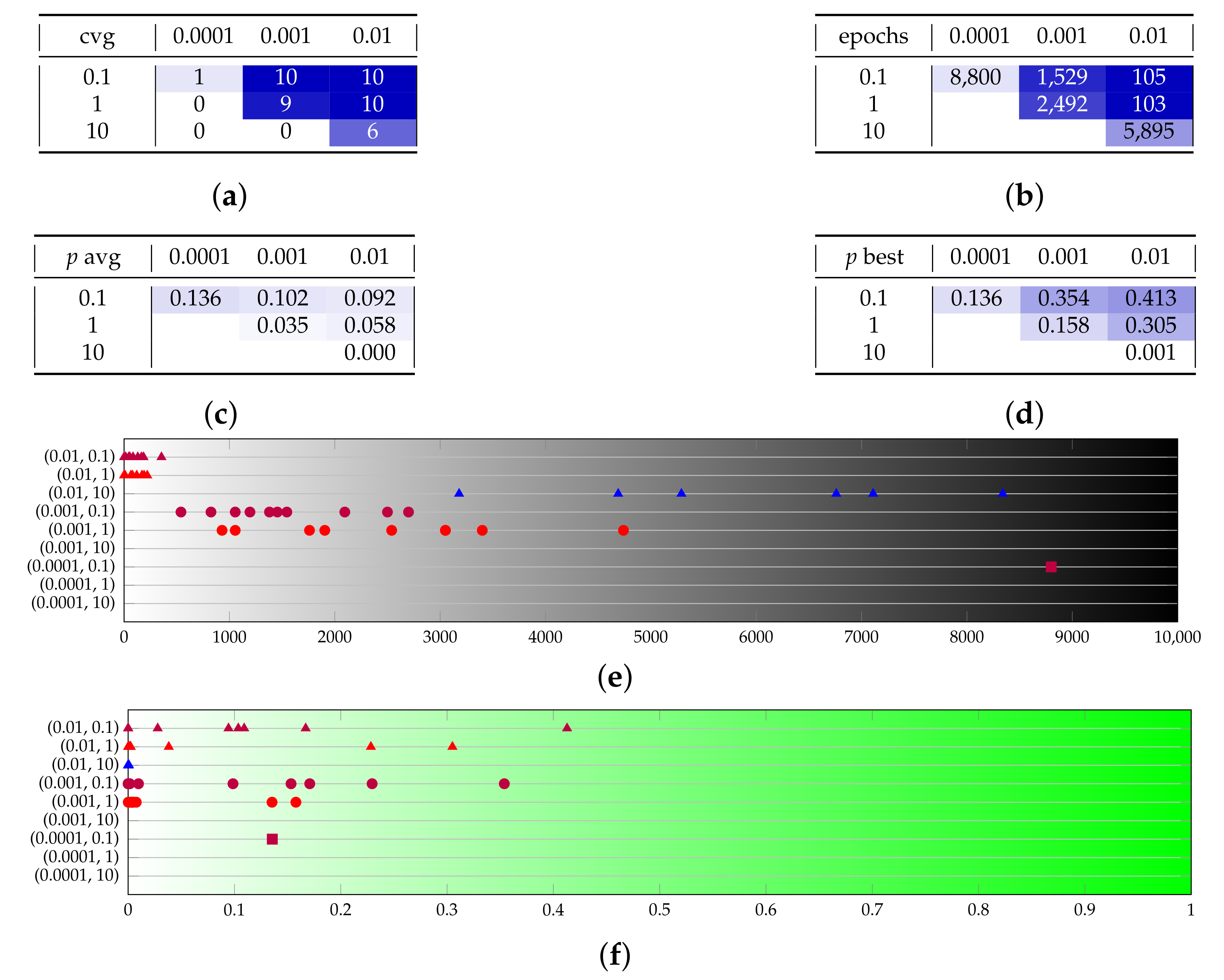
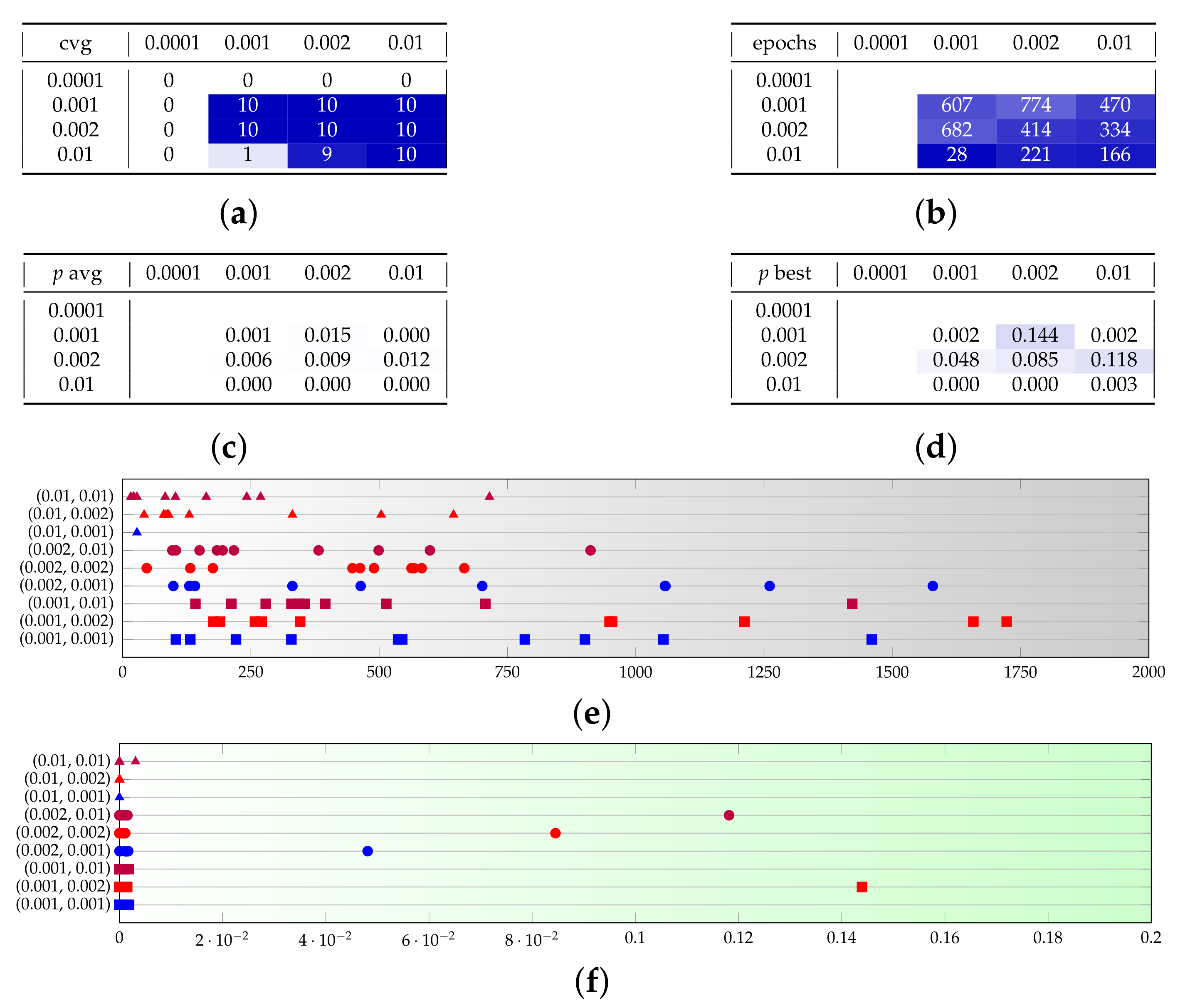
Let us now introduce the evaluation of the SPSA optimizer. Test set F (in Figure A7) shows the effect of the adoption of SPSA in the generator and Adam in the discriminator. We extended the maximum allowed numbers of epochs to 10,000, taking into account that each epoch is faster with SPSA; see Section 5.4. With SPSA in the generator, we get to convergence in a very small number of epochs if we choose the optimal learning rate of and perturbation of . Unluckily, this result is obtained at the expense of a degraded quality: with SPSA, the average p-value hardly goes above 0.1, and we have no example of any good spike. The test set G (in Figure A8) shows the effect of different shot numbers; no remarkable effect can be observed.
Figure A7.
Test set F provides a sensitivity analysis on the parameters for SPSA in the generator. (a–d) The rows represent the ratio between learning rate and perturbation factor, and the columns represent the generator learning rate. (e,f) The couples on the vertical axis are . Marker shapes represent the learning rate and marker colors represent the ratio. (a) Converging runs, out of 10. (b) Number of epochs before convergence, on average. (c) p-value for the test once convergence is reached (average over converging runs). (d) p-value for the test once convergence is reached (best run). (e) Visual representation of the epochs before convergence. (f) Visual representation of the p-value.

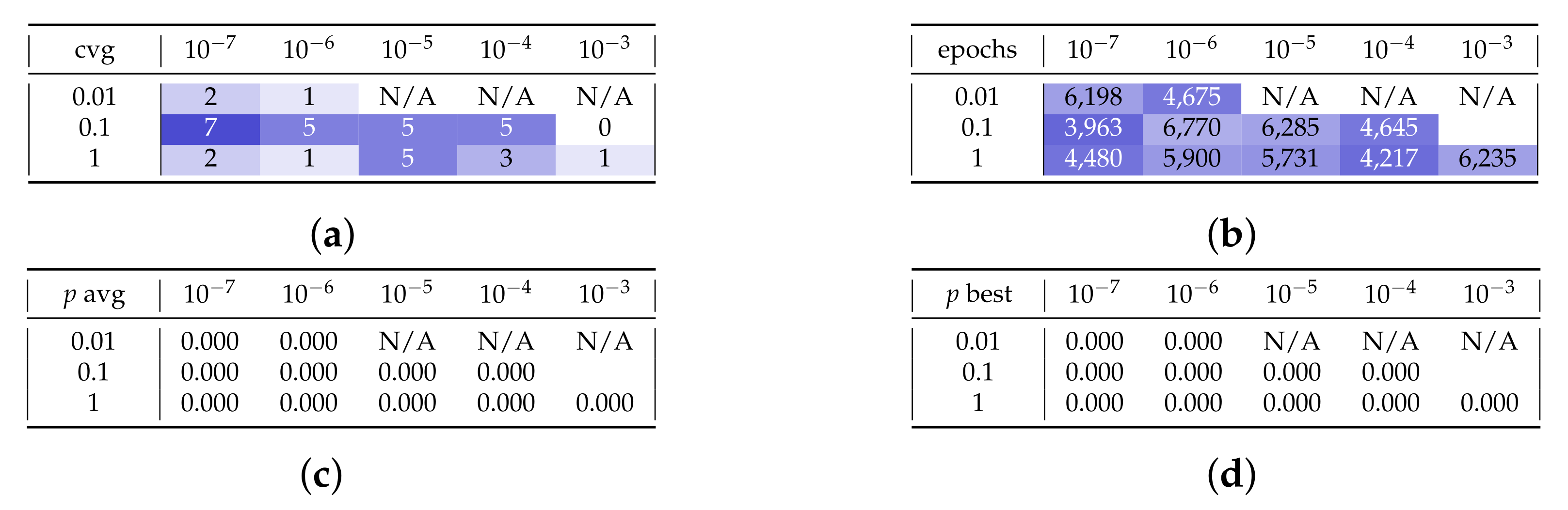
If we conversely use SPSA in the discriminator and Adam in the generator, as shown in the test set H (Figure A9 and Figure A10), the solution quality degrades to a point that we consider unacceptable.
Next, we turn to the case of qubits. Starting again with Adam for both the generator and the discriminator, in the test set J (Figure A11) we set the learning rate to and we experiment with different values of and . The p-values obtained are in the order of , significantly worse than the ones we obtained for ; indeed, all plots dealing with the p-value for are rescaled in the interval . By simply looking at average and best values in Figure A11c,d, respectively, appears as a particularly good choice, but with a deeper look to Figure A11f, this is due to a single, spiky run, resulting in the effect of a particularly favorable random initialization: indeed, the average p-value of the other nine runs with is below , in line with the other experiments.
Figure A8.
Test set G provides a sensitivity analysis on the number of shots s, with SPSA in the generator. (a) Converging runs, out of 10. (b) Number of epochs before convergence, on average. (c) p-value for the test once convergence is reached (average over converging runs). (d) p-value for the test once convergence is reached (best run). (e) Visual representation of the epochs before convergence. (f) Visual representation of the p-value.

Figure A9.
Test set H provides a sensitivity analysis on the parameters for SPSA in the discriminator. The rows represent the ratio between learning rate and perturbation factor, and the columns represent the learning rate. (a) Converging runs, out of 10. Experiments marked with N/A were excluded from the test set. (b) Number of epochs before convergence, on average. (c) p-value for the test once convergence is reached (average over converging runs). (d) p-value for the test once convergence is reached (best run).

Figure A10.
Test set I provides a sensitivity analysis on the number of shots s, with SPSA in the discriminator. (a) Converging runs, out of 10. (b) Number of epochs before convergence, on average. (c) p-value for the test once convergence is reached (average over converging runs). (d) p-value for the test once convergence is reached (best run).

Additionally, we pick and we make a sensitivity analysis over the learning rates. The test set K (in Figure A12) shows the outcomes. On one hand, it is clear that too small values of the learning rates lead to no convergence. On the other hand, large values, especially in the generator, lead to poor quality. The best accuracy can be achieved with a learning rate for the generator between and and for the discriminator, between and .
Finally, test set J (in Figure A13) deals with the number of shots: increasing s, it reaches better accuracy. Let us remark again that achieving good quality for is very rare: besides any fine tuning of the hyper-parameters, the most relevant protocol to achieve good outcomes is simply that of repeating experiments with different random initial points.
Figure A11.
Test set J provides a sensitivity analysis on the discriminator size for . (a–d) The rows represent and the columns . (e,f) The couples on the vertical axis are . The marker shapes represent and marker colors represent . (a) Converging runs, out of 10. (b) Number of epochs before convergence, on average. (c) p-value for the test once convergence is reached (average over converging runs). (d) p-value for the test once convergence is reached (best run). (e) Visual representation of the epochs before convergence. (f) Visual representation of the p-value, zoomed on as no points have .

Figure A12.
Test set K provides a sensitivity analysis on the learning rates for Adam, qubits. (a–d) The rows represent the generator learning rate, and the columns represent the discriminator learning rate. (e,f) The couples on the vertical axis are . The marker shapes represent and marker colors represent . (a) Converging runs, out of 10. (b) Number of epochs before convergence, on average. (c) p-value for the test once convergence is reached (average over converging runs). (d) p-value for the test once convergence is reached (best run). (e) Visual representation of the epochs before convergence. (f) Visual representation of the p-value, zoomed on , as no points have .

Figure A13.
Test set L provides a sensitivity analysis on the number of shots s for qubits. (a) Converging runs, out of 10. (b) Number of epochs before convergence, on average. (c) p-value for the test once convergence is reached (average over converging runs). (d) p-value for the test once convergence is reached (best run). (e) Visual representation of the epochs before convergence. (f) Visual representation of the p-value, zoomed on as no points have .

Appendix B. Additional Remarks on the Isolation of the Best Run
As stated, the best runs with Adam AMSGRAD obtain p-values greater than 0.8, remarkably separated from sub-optimal runs, whose p-values lie under 0.6. An early identification of the best runs during the training would allow to iteratively restart the process in order to increase the success rate. Consequently, we are interested in understanding if any feature of the training process can be used as a predictor.
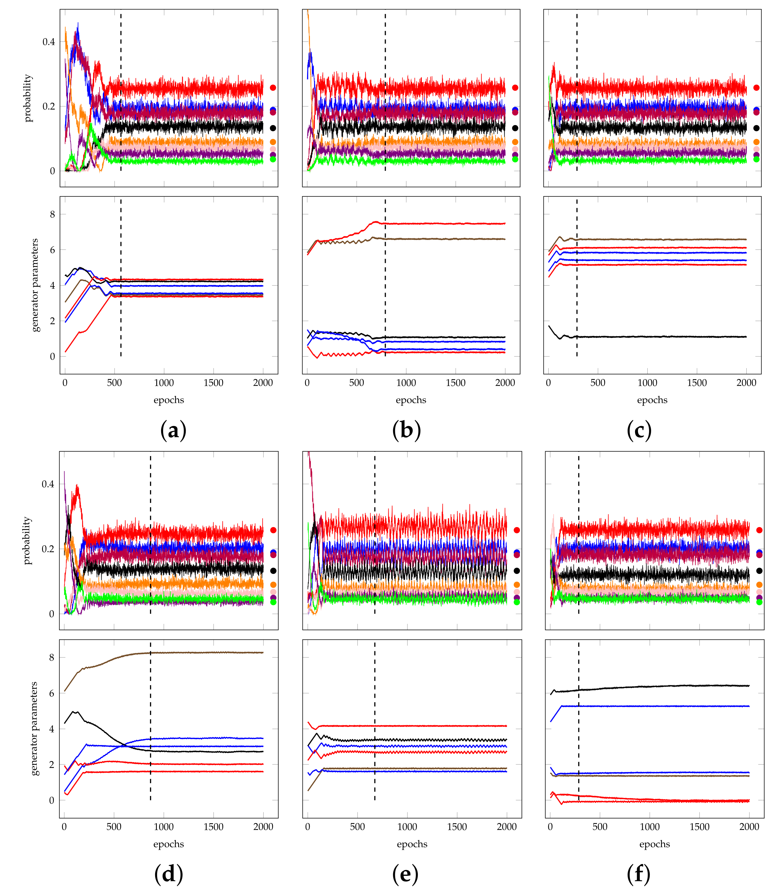
As a qualitative study case, we focus on the case from test set B, visualized by the red pentagons in Figure A2f. The case is interesting because there is a relevant number of optimal runs, namely three. Figure A14 represents the training process of the three optimal cases (achieving a p-value of 0.9450, 0.9163, and 0.9016, respectively) and of three archetype sub-optimal cases (with p-values 0.3029, 0.2744, and 0.3610, respectively). The analysis suggests that optimal runs have an elbow in the parameters right at the time of convergence, while sub-optimal runs have either slow convergence, oscillatory behaviors around the convergence value, or residual dynamics after convergence.
Figure A14.
Focus on experiments from test set B. In each couple of plots, the one above represents the evolution of the trained PDF, while the one below contains the evolution of parameters, as in Figure 3. (a–c) The optimal runs. (d–f) Examples of sub-optimal runs. Vertical dashed lines mark the convergence epoch, as detected by our rule (refer to Section 5.2). (a) An optimal case, with an elbow in the parameters at convergence time. (b) Another optimal case, with similar behavior. (c) The third optimal run, with a less characterized behavior. (d) A sub-optimal run characterized by slow convergence. (e) A sub-optimal run characterized by oscillations. (f) A sub-optimal run with non-steady parameters after convergence.

References
- Grover, L.K. Synthesis of Quantum Superpositions by Quantum Computation. Phys. Rev. Lett. 2000, 85, 1334–1337. [Google Scholar] [CrossRef] [PubMed]
- Grover, L.; Rudolph, T. Creating superpositions that correspond to efficiently integrable probability distributions. arXiv 2002, arXiv:quant-ph/0208112. [Google Scholar]
- Mitarai, K.; Kitagawa, M.; Fujii, K. Quantum Analog-Digital Conversion. Phys. Rev. 2019, 99, 012301. [Google Scholar] [CrossRef] [Green Version]
- Sanders, Y.R.; Low, G.H.; Scherer, A.; Berry, D.W. Black-box quantum state preparation without arithmetic. Phys. Rev. Lett. 2019, 122, 020502. [Google Scholar] [CrossRef] [Green Version]
- Aaronson, S. Read the fine print. Nat. Phys. 2015, 11, 291–293. [Google Scholar] [CrossRef]
- Giovannetti, V.; Lloyd, S.; Maccone, L. Architectures for a quantum random access memory. Phys. Rev. 2008, 78, 052310. [Google Scholar] [CrossRef] [Green Version]
- Le, P.Q.; Dong, F.; Hirota, K. A flexible representation of quantum images for polynomial preparation, image compression, and processing operations. Quantum Inf. Process. 2011, 10, 63–84. [Google Scholar] [CrossRef]
- Zoufal, C.; Lucchi, A.; Woerner, S. Quantum Generative Adversarial Networks for Learning and Loading Random Distributions. Npj Quantum Inf. 2019, 5, 103. [Google Scholar] [CrossRef] [Green Version]
- Nakaji, K.; Uno, S.; Suzuki, Y.; Raymond, R.; Onodera, T.; Tanaka, T.; Tezuka, H.; Mitsuda, N.; Yamamoto, N. Approximate amplitude encoding in shallow parameterized quantum circuits and its application to financial market indicator. arXiv 2021, arXiv:2103.13211. [Google Scholar]
- Niu, M.Y.; Zlokapa, A.; Broughton, M.; Boixo, S.; Mohseni, M.; Smelyanskyi, V.; Neven, H. Entangling Quantum Generative Adversarial Networks. arXiv 2021, arXiv:2105.00080. [Google Scholar]
- Goodfellow, I.; Pouget-Abadie, J.; Mirza, M.; Xu, B.; Warde-Farley, D.; Ozair, S.; Courville, A.; Bengio, Y. Generative adversarial networks. Commun. ACM 2020, 63, 139–144. [Google Scholar] [CrossRef]
- Gui, J.; Sun, Z.; Wen, Y.; Tao, D.; Ye, J. A Review on Generative Adversarial Networks: Algorithms, Theory, and Applications. arXiv 2020, arXiv:2001.06937. [Google Scholar] [CrossRef]
- Stamatopoulos, N.; Egger, D.J.; Sun, Y.; Zoufal, C.; Iten, R.; Shen, N.; Woerner, S. Option Pricing using Quantum Computers. Quantum 2020, 4, 291. [Google Scholar] [CrossRef]
- Agliardi, G.; Grossi, M.; Pellen, M.; Prati, E. Quantum integration of elementary particle processes. arXiv 2022, arXiv:2201.01547. [Google Scholar]
- Havlíček, V.; Córcoles, A.D.; Temme, K.; Harrow, A.W.; Kandala, A.; Chow, J.M.; Gambetta, J.M. Supervised learning with quantum-enhanced feature spaces. Nature 2019, 567, 209–212. [Google Scholar] [CrossRef] [Green Version]
- Torrontegui, E.; García-Ripoll, J.J. Unitary quantum perceptron as efficient universal approximator. Epl. Europhys. Lett. 2019, 125, 30004. [Google Scholar] [CrossRef] [Green Version]
- Maronese, M.; Prati, E. A continuous rosenblatt quantum perceptron. Int. J. Quantum Inf. 2021, 98, 2140002. [Google Scholar] [CrossRef]
- Maronese, M.; Destri, C.; Prati, E. Quantum activation functions for quantum neural networks. arXiv 2022, arXiv:2201.03700. [Google Scholar]
- Wan, K.H.; Dahlsten, O.; Kristjánsson, H.; Gardner, R.; Kim, M.S. Quantum generalisation of feedforward neural networks. NPJ Quantum Inf. 2017, 3, 1–8. [Google Scholar] [CrossRef] [Green Version]
- Shao, C. A quantum model of feed-forward neural networks with unitary learning algorithms. Quantum Inf. Process. 2020, 19, 102. [Google Scholar] [CrossRef]
- Fujii, K.; Nakajima, K. Quantum Reservoir Computing: A Reservoir Approach Toward Quantum Machine Learning on Near-Term Quantum Devices. In Reservoir Computing; Nakajima, K., Fischer, I., Eds.; Natural Computing Series; Springer: Singapore, 2021; pp. 423–450. [Google Scholar] [CrossRef]
- Lazzarin, M.; Galli, D.E.; Prati, E. Multi-class quantum classifiers with tensor network circuits for quantum phase recognition. arXiv 2021, arXiv:2110.08386. [Google Scholar]
- Rocutto, L.; Destri, C.; Prati, E. Quantum Semantic Learning by Reverse Annealing of an Adiabatic Quantum Computer. Adv. Quantum Technol. 2021, 4, 2000133. [Google Scholar] [CrossRef]
- Rocutto, L.; Prati, E. A complete restricted Boltzmann machine on an adiabatic quantum computer. Int. J. Quantum Inf. 2021, 19, 2141003. [Google Scholar] [CrossRef]
- Dallaire-Demers, P.L.; Killoran, N. Quantum generative adversarial networks. Phys. Rev. 2018, 98, 012324. [Google Scholar] [CrossRef] [Green Version]
- Huang, H.L.; Du, Y.; Gong, M.; Zhao, Y.; Wu, Y.; Wang, C.; Li, S.; Liang, F.; Lin, J.; Xu, Y.; et al. Experimental Quantum Generative Adversarial Networks for Image Generation. Phys. Rev. Appl. 2021, 16, 024051. [Google Scholar] [CrossRef]
- Stein, S.A.; Baheri, B.; Chen, D.; Mao, Y.; Guan, Q.; Li, A.; Fang, B.; Xu, S. QuGAN: A Generative Adversarial Network Through Quantum States. arXiv 2021, arXiv:2010.09036. [Google Scholar]
- Montanaro, A. Quantum speedup of Monte Carlo methods. Proceedings. Math. Phys. Eng. Sci. 2015, 471, 20150301. [Google Scholar] [CrossRef] [Green Version]
- Suzuki, Y.; Uno, S.; Raymond, R.; Tanaka, T.; Onodera, T.; Yamamoto, N. Amplitude estimation without phase estimation. Quantum Inf. Process. 2020, 19, 75. [Google Scholar] [CrossRef] [Green Version]
- Grinko, D.; Gacon, J.; Zoufal, C.; Woerner, S. Iterative Quantum Amplitude Estimation. NPJ Quantum Inf. 2021, 7, 52. [Google Scholar] [CrossRef]
- Egger, D.J.; Gutiérrez, R.G.; Mestre, J.C.; Woerner, S. Credit risk analysis using quantum computers. IEEE Trans. Comput. 2021, 70, 2136–2145. [Google Scholar] [CrossRef]
- Harrow, A.W.; Hassidim, A.; Lloyd, S. Quantum Algorithm for Linear Systems of Equations. Phys. Rev. Lett. 2009, 103, 150502. [Google Scholar] [CrossRef] [PubMed]
- Rebentrost, P.; Gupt, B.; Bromley, T.R. Quantum computational finance: Monte Carlo pricing of financial derivatives. Phys. Rev. 2018, 98, 022321. [Google Scholar] [CrossRef] [Green Version]
- Pérez-Salinas, A.; Cervera-Lierta, A.; Gil-Fuster, E.; Latorre, J.I. Data re-uploading for a universal quantum classifier. Quantum 2020, 4, 226. [Google Scholar] [CrossRef]
- Preskill, J. Quantum Computing in the NISQ era and beyond. Quantum 2018, 2, 79. [Google Scholar] [CrossRef]
- Boixo, S.; Isakov, S.V.; Smelyanskiy, V.N.; Babbush, R.; Ding, N.; Jiang, Z.; Bremner, M.J.; Martinis, J.M.; Neven, H. Characterizing Quantum Supremacy in Near-Term Devices. Version: 3. Nat. Phys. 2018, 14, 595–600. [Google Scholar] [CrossRef]
- Aaronson, S.; Chen, L. Complexity-Theoretic Foundations of Quantum Supremacy Experiments. arXiv 2016, arXiv:1612.05903. [Google Scholar]
- Pednault, E.; Gunnels, J.A.; Nannicini, G.; Horesh, L.; Magerlein, T.; Solomonik, E.; Draeger, E.W.; Holland, E.T.; Wisnieff, R. Pareto-Efficient Quantum Circuit Simulation Using Tensor Contraction Deferral. arXiv 2020, arXiv:1710.05867. [Google Scholar]
- Peruzzo, A.; McClean, J.; Shadbolt, P.; Yung, M.H.; Zhou, X.Q.; Love, P.J.; Aspuru-Guzik, A.; O’Brien, J.L. A variational eigenvalue solver on a photonic quantum processor. Nat. Commun. 2014, 5, 4213. [Google Scholar] [CrossRef] [Green Version]
- McClean, J.R.; Romero, J.; Babbush, R.; Aspuru-Guzik, A. The theory of variational hybrid quantum-classical algorithms. New J. Phys. 2016, 18, 023023. [Google Scholar] [CrossRef]
- Cortese, J.A.; Braje, T.M. Loading Classical Data into a Quantum Computer. arXiv 2018, arXiv:1803.01958. [Google Scholar]
- Shende, V.V.; Bullock, S.S.; Markov, I.L. Synthesis of Quantum Logic Circuits. IEEE Trans. Comput.-Aided Des. Integr. Circuits Syst. 2006, 25, 1000–1010. [Google Scholar] [CrossRef] [Green Version]
- Kerenidis, I.; Prakash, A. Quantum Recommendation Systems. arXiv 2016, arXiv:1603.08675. [Google Scholar]
- Hann, C.T.; Zou, C.L.; Zhang, Y.; Chu, Y.; Schoelkopf, R.J.; Girvin, S.; Jiang, L. Hardware-Efficient Quantum Random Access Memory with Hybrid Quantum Acoustic Systems. Phys. Rev. Lett. 2019, 123, 250501. [Google Scholar] [CrossRef] [PubMed] [Green Version]
- Lloyd, S.; Weedbrook, C. Quantum Generative Adversarial Learning. Phys. Rev. Lett. 2018, 121, 040502. [Google Scholar] [CrossRef] [PubMed] [Green Version]
- Bharti, K.; Cervera-Lierta, A.; Kyaw, T.H.; Haug, T.; Alperin-Lea, S.; Anand, A.; Degroote, M.; Heimonen, H.; Kottmann, J.S.; Menke, T.; et al. Noisy intermediate-scale quantum (NISQ) algorithms. arXiv 2021, arXiv:2101.08448. [Google Scholar]
- Schuld, M.; Sinayskiy, I.; Petruccione, F. The quest for a Quantum Neural Network. Quantum Inf. Process. 2014, 13, 2567–2586. [Google Scholar] [CrossRef] [Green Version]
- Biamonte, J.; Wittek, P.; Pancotti, N.; Rebentrost, P.; Wiebe, N.; Lloyd, S. Quantum Machine Learning. Nature 2017, 549, 195–202. [Google Scholar] [CrossRef] [PubMed]
- Coyle, B.; Henderson, M.; Le, J.C.J.; Kumar, N.; Paini, M.; Kashefi, E. Quantum versus Classical Generative Modelling in Finance. arXiv 2020, arXiv:2008.00691. [Google Scholar] [CrossRef]
- Cerezo, M.; Arrasmith, A.; Babbush, R.; Benjamin, S.C.; Endo, S.; Fujii, K.; McClean, J.R.; Mitarai, K.; Yuan, X.; Cincio, L.; et al. Variational Quantum Algorithms. arXiv 2020, arXiv:2012.09265. [Google Scholar] [CrossRef]
- Cheng, S.; Chen, J.; Wang, L. Information Perspective to Probabilistic Modeling: Boltzmann Machines versus Born Machines. Entropy 2018, 20, 583. [Google Scholar] [CrossRef] [Green Version]
- Abraham, H.; Akhalwaya, I.Y.; Aleksandrowicz, G.; Alexander, T.; Alexandrowics, G.; Arbel, E.; Asfaw, A.; Azaustre, C.; AzizNgoueya, P.B.; Barron, G. Qiskit: An open-source framework for quantum computing. Zenodo 2019, 2562111. [Google Scholar]
- SciPy User Guide–SciPy v1.7.1 Manual. Available online: https://docs.scipy.org/doc/scipy/reference/ (accessed on 24 January 2022).
- Benedetti, M.; Lloyd, E.; Sack, S.; Fiorentini, M. Parameterized quantum circuits as machine learning models. Quantum Sci. Technol. 2019, 4, 043001. [Google Scholar] [CrossRef] [Green Version]
- Gacon, J.; Zoufal, C.; Carleo, G.; Woerner, S. Simultaneous Perturbation Stochastic Approximation of the Quantum Fisher Information. Quantum 2021, 5, 567. [Google Scholar] [CrossRef]
- McClean, J.R.; Boixo, S.; Smelyanskiy, V.N.; Babbush, R.; Neven, H. Barren plateaus in quantum neural network training landscapes. Nat. Commun. 2018, 9, 4812. [Google Scholar] [CrossRef] [PubMed] [Green Version]
- Cerezo, M.; Sone, A.; Volkoff, T.; Cincio, L.; Coles, P.J. Cost function dependent barren plateaus in shallow parametrized quantum circuits. Nat. Commun. 2021, 12, 1791. [Google Scholar] [CrossRef]
- Wang, S.; Fontana, E.; Cerezo, M.; Sharma, K.; Sone, A.; Cincio, L.; Coles, P.J. Noise-Induced Barren Plateaus in Variational Quantum Algorithms. arXiv 2021, arXiv:2007.14384. [Google Scholar] [CrossRef] [PubMed]
- Abbas, A.; Sutter, D.; Zoufal, C.; Lucchi, A.; Figalli, A.; Woerner, S. The power of quantum neural networks. Nat. Comput. Sci. 2021, 1, 403–409. [Google Scholar] [CrossRef]
- Arrasmith, A.; Cerezo, M.; Czarnik, P.; Cincio, L.; Coles, P.J. Effect of barren plateaus on gradient-free optimization. Quantum 2021, 5, 558. [Google Scholar] [CrossRef]
- torch.optim—PyTorch 1.8.1 Documentation. Available online: https://pytorch.org/docs/stable/optim.html(accessed on 6 January 2022).
- Nagarajan, V.; Raffel, C.; Goodfellow, I.J. Theoretical Insights into Memorization in GANs; Neural Information Processing Systems Workshop: Montréal, QC, Canada, 2018; Volume 1. [Google Scholar]
Figure 1.
The training of a qGAN alternates the training of the generator and of the discriminator. The generator training has access to both the generator and the discriminator, but not to true data. Conversely, the discriminator training has no direct access to the generator, as it works by comparing generated data with true data. Quantum data are marked by a Bloch sphere. (a) In the case of a qGAN, the generator is an ansatz parametric quantum circuit. It produces a quantum state, in which squared amplitudes encode approximate probabilities. After measurement , it produces samples according to approximate probabilities. (b) A discriminator is a neural network that labels a sample as true or fake. (c) The training of a qGAN alternates the training of the generator and of the discriminator. The generator training has access to both the generator and the discriminator, but not to true data. Conversely, the discriminator training has no direct access to the generator, as it works by comparing generated data with true data. Quantum data are marked by a Bloch sphere. (d) The ansatz is a layered quantum circuit based on qubits. Here, the ansatz for the case of qubits and repetitions is shown. Rotation layers are composed of gates, while entanglement layers are made of . (e) The discriminative network is a classical deep neural network with two hidden layers. Activation functions are Leaky ReLU for the intermediate nodes, and a sigmoid for the output.

Figure 2.
Visualization of the trade-off between training complexity and quality, for the test cases listed in Table 2. On the vertical axis, the complexity, calculated according to Equations (8) and (9). On the horizontal axis, the p-value of the test after training is a metric for accuracy. Each dot represents a test execution, whereas dots with the same color are the result of different random initializations obtained with the same hyper-parameters. Tests are the same across the three plots. The best runs are in the bottom right corner of each plot since they have high accuracy and low computational cost. Each ellipse is a synthetic representation of the respective scenario: its center corresponds to the average of the converging runs in the scenario, and its radii correspond to the standard deviations. (a) Classical training complexity vs. quality. (b) Detail of subfigure (a). Here, test case (b) was excluded to allow rescaling in the vertical axis. (c) Quantum training complexity vs. quality.

Figure 3.
Different training processes, obtained with different hyper-parameters and different initial random conditions. In all plots, the horizontal axis represents training time. In the top plots, each color is related to a value of the discretized random variable, the lines represent the probability density of the generated distribution, and the circles on the right represent the target distribution. In the bottom plots, the evolution of the ansatz parameters during the training. Vertical dashed lines mark the convergence epoch j, according to our convention. More details on how runs are generated can be found in Table A3. (a) A divergent run: parameters (in the bottom plot) do not stabilize. (b) A convergent run, with strong oscillations in the generator parameters and in the resulting distribution. (c) A convergent run, with poor solution quality: in the top plot, e.g., the red line and blue line are far from the target circles. (d) A convergent run achieving a good quality of the solution.

Figure 4.
The test conducted to test the null hypothesis of the generated distribution to be independent and identically distributed like the target distribution. The plot is created by testing samples taken from the same generated distribution against the same target distribution, and varying the number of samples s.

Table 1.
Three different ways to encode the data set into a quantum state. is the number of qubits needed for the index.
Table 1.
Three different ways to encode the data set into a quantum state. is the number of qubits needed for the index.
| Encoding | Form | Number of Qubits | Data Type of Each Item | Algorithms |
|---|---|---|---|---|
| Multi-register | Any binary string of length m (including integer, fixed point, and floating point numbers). In literature, a common choice for numbers is fixed point. | Quantum arithmetic (adder, multiplier, max,…) | ||
| Digital | Any binary string of length m (including integer, fixed point, and floating point numbers). In literature, a common choice for numbers is fixed point. | Grover | ||
| Analog | n | Complex numbers satisfying the constraint . | Quantum Fourier Transform (QFT), HHL |
| Case | n | k | Generator | Discriminator | Shots | ||
|---|---|---|---|---|---|---|---|
| a. Baseline | 3 | 1 | 8 | 8 | Adam, lr = , = 0.7, = 0.99 | Adam, lr = , = 0.7, = 0.99 | 2000 |
| b. Big discriminator size | 3 | 1 | 128 | 128 | Adam, lr = , = 0.7, = 0.99 | Adam, lr = , = 0.7, = 0.99 | 2000 |
| c. Low generator learning rate | 3 | 1 | 8 | 8 | Adam, lr = , = 0.7, = 0.99 | Adam, lr = , = 0.7, = 0.99 | 2000 |
| d. Many shots | 3 | 1 | 8 | 8 | Adam, lr = , = 0.7, = 0.99 | Adam, lr = , = 0.7, = 0.99 | 8000 |
| e. SPSA in generator | 3 | 1 | 8 | 8 | SPSA, lr = , perturbation = | Adam, lr = , = 0.7, = 0.99 | 2000 |
Publisher’s Note: MDPI stays neutral with regard to jurisdictional claims in published maps and institutional affiliations. |
© 2022 by the authors. Licensee MDPI, Basel, Switzerland. This article is an open access article distributed under the terms and conditions of the Creative Commons Attribution (CC BY) license (https://creativecommons.org/licenses/by/4.0/).
Share and Cite
MDPI and ACS Style
Agliardi, G.; Prati, E. Optimal Tuning of Quantum Generative Adversarial Networks for Multivariate Distribution Loading. Quantum Rep. 2022, 4, 75-105. https://doi.org/10.3390/quantum4010006
AMA Style
Agliardi G, Prati E. Optimal Tuning of Quantum Generative Adversarial Networks for Multivariate Distribution Loading. Quantum Reports. 2022; 4(1):75-105. https://doi.org/10.3390/quantum4010006
Chicago/Turabian StyleAgliardi, Gabriele, and Enrico Prati. 2022. "Optimal Tuning of Quantum Generative Adversarial Networks for Multivariate Distribution Loading" Quantum Reports 4, no. 1: 75-105. https://doi.org/10.3390/quantum4010006