
Flow Annealed Kalman Inversion for Gradient-Free Inference in Bayesian Inverse Problems †


1
Department of Astronomy, Tsinghua University, Beijing 100084, China
2
Berkeley Center for Cosmological Physics and Department of Physics, University of California, Berkeley, CA 94720, USA
3
Physics Department, Lawrence Berkeley National Laboratory, Cyclotron Rd, Berkeley, CA 94720, USA
*
Author to whom correspondence should be addressed.
†
Presented at the 42nd International Workshop on Bayesian Inference and Maximum Entropy Methods in Science and Engineering, Garching, Germany, 3–7 July 2023.
Phys. Sci. Forum 2023, 9(1), 21; https://doi.org/10.3390/psf2023009021
Published: 4 January 2024
(This article belongs to the Proceedings of The 42nd International Workshop on Bayesian Inference and Maximum Entropy Methods in Science and Engineering)
Abstract
:For many scientific inverse problems, we are required to evaluate an expensive forward model. Moreover, the model is often given in such a form that it is unrealistic to access its gradients. In such a scenario, standard Markov Chain Monte Carlo algorithms quickly become impractical, requiring a large number of serial model evaluations to converge on the target distribution. In this paper, we introduce Flow Annealed Kalman Inversion (FAKI). This is a generalization of Ensemble Kalman Inversion (EKI) where we embed the Kalman filter updates in a temperature annealing scheme and use normalizing flows (NFs) to map the intermediate measures corresponding to each temperature level to the standard Gaussian. Thus, we relax the Gaussian ansatz for the intermediate measures used in standard EKI, allowing us to achieve higher-fidelity approximations to non-Gaussian targets. We demonstrate the performance of FAKI on two numerical benchmarks, showing dramatic improvements over standard EKI in terms of accuracy whilst accelerating its already rapid convergence properties (typically in steps).
1. Introduction
Many scientific inference tasks are concerned with inverse problems of the form
where are the data, are the model parameters, is the forward map, and is the observation noise. Throughout this work, we will assume that we do not have access to gradients of with respect to the parameters, and that , where is a fixed noise covariance. The assumption of additive Gaussian noise is the standard setting for Ensemble Kalman Inversion (EKI) [1,2,3,4,5,6,7,8], and whilst we are restricted to problems with Gaussian likelihoods, this covers a large family of scientific inverse problems. The goal of the Bayesian inverse problem is then to recover the posterior distribution over the model parameters given our observations, .
Typical gradient-free inference methods often involve some variant on Markov Chain Monte Carlo (MCMC) algorithms, e.g., random walk Metropolis [9,10,11] or Sequential Monte Carlo (SMC) [12]. However, these methods typically require serial model evaluations to achieve convergence, making them intractable for problems with expensive forward models. In contrast, EKI utilizes embarrassingly parallel model evaluations to update parameter estimates, typically converging to an approximate solution in iterations [2,6,7,8].
EKI leverages ideas originally developed in the context of Ensemble Kalman Filtering (EKF) for data assimilation [13]. Since its development, EKI has seen applications across a range of disciplines, including studies of fluid flow [14], climate models [15], and machine learning tasks [16]. EKI can be understood in the context of annealing, where we seek to move from the prior to the posterior through a sequence of intermediate measures. In standard EKI, this involves constructing a sequence of Gaussian approximations to the intermediate measures. In the regime where we have a Gaussian prior and a linear forward model , the particle distribution obtained via EKI converges to the true posterior in the limit where the ensemble size . However, outside this linear Gaussian regime, EKI is an uncontrolled approximation to the posterior that is constructed on the basis of matching first and second moments of the target distribution. Nonetheless, EKI has been shown to perform well on problems with non-linear forward models and slightly non-Gaussian targets [1,2,6].
In this work, we propose the application of normalizing flows (NFs) [17,18,19,20] to relax the Gaussian ansatz made by standard EKI for the intermediate measures. Instead of assuming a Gaussian particle distribution at each iteration, the NF is used to fit the empirical particle distribution and map it to a Gaussian latent space, where the EKI updates are performed. Thus, we are better able to capture non-Gaussian target geometries. The structure of this paper is as follows: in Section 2 we describe the Flow Annealed Kalman Inversion (FAKI) algorithm; in Section 3, we demonstrate the performance of the method on two Bayesian inference tasks with non-Gaussian target geometries; and we summarize our work in Section 4.
2. Methods
2.1. Regularized Ensemble Kalman Inversion
A number of versions of EKI have been proposed in the literature. Of interest here is the regularized, perturbed observation form of EKI [6]. Starting with an ensemble of particles drawn from the prior, , the particles are updated at each iteration according to
The empirical covariances and are given by
At each iteration, we perturb the forward model evaluations with the Gaussian observation noise . The parameter is a Tikhonov regularization parameter, which can be viewed as an inverse step size in the Bayesian annealing context. In particular, given a set of annealing parameters , we have the corresponding set of target distributions
with
EKI proceeds by constructing a sequence of ensemble approximations to Gaussian distributions that approximate the intermediate targets.
The choice of the regularization parameter, , controls the transition from the prior to the posterior. Previous proposals for an adaptive choice have taken inspiration from SMC by using a threshold on the effective sample size (ESS) of the particles at each temperature level [21,22]. In this work, we adopt the same approach, calculating pseudo-importance weights at each temperature given by
The next temperature level can then be selected by solving
using the bisection method, where is the target fractional ESS threshold. Throughout our work we set . The full pseudo-code for EKI is given in Algorithm 1.
| Algorithm 1 Ensemble Kalman Inversion |
|
2.2. Normalizing Flows
As discussed above, standard EKI proceeds by constructing a sequence of ensemble approximations to Gaussian distributions. The procedure works well in the situation where the target and all the intermediate measures are close to Gaussian. However, when any of these measures are far from Gaussian, EKI can dramatically fail to capture the final target geometry.
To address this shortcoming, we propose the use of NFs to approximate each intermediate target, instead of using the Gaussian ansatz of standard EKI. NFs are powerful generative models that can be used for flexible density estimation and sampling [17,18,19,20]. An NF model maps from the original space to a latent space through a sequence of invertible transformations , such that we have a bijective mapping . The mapping is such that the latent variables are mapped to some simple base distribution, typically chosen to be the standard Normal distribution, giving .
The NF density can be evaluated through the change of variables formula,
where denotes the Jacobian of f. The efficient evaluation of this density requires the Jacobian of the transformation to be easy to evaluate, and efficient sampling requires the inverse of the mapping f to be easy to calculate. In this work, we use Masked Autoregressive Flows (MAFs) [18], which have previously been found to perform well in the context of preconditioned MCMC sampling within SMC without the need for expensive hyper-parameter searches during sampling [23].
2.3. Flow Annealed Kalman Inversion
Given particles distributed as , the subsequent target can be written as
We may therefore view , i.e., the posterior at the temperature level , as an effective prior for , with a data likelihood annealed by . By fitting an NF to the particles , we obtain an approximate map from the intermediate target to . The latent space target is then given by the change of variables formula as
By controlling the choice of , we control the distance between the Gaussianized effective prior and this latent space target density. For FAKI, we therefore perform the EKI updates in the NF latent space at each temperature level, allowing us to relax the Gaussian ansatz of standard EKI by constructing an approximate map from each to a Gaussian latent space. It is worth noting that, whilst this method relaxes the Gaussianity assumptions of standard EKI, it does not address the linearity assumptions used in deriving EKI.
The FAKI update for the latent space particle locations is given by
where the latent space empirical covariances are given by
The full pseudocode for FAKI is given in Algorithm 2.
| Algorithm 2 Flow Annealed Kalman Inversion |
|
3. Results
In this section, we demonstrate the performance of FAKI compared to standard EKI on two numerical benchmarks, a two-dimensional Rosenbrock distribution and a stochastic Lorenz system [24,25]. Both models display significant non-Gaussianity at some point during the transition from prior to posterior, severely frustrating the performance of EKI. This manifests in both the reduced fidelity of the final ensemble approximations to the posterior and a larger number of iterations being required for convergence following the ESS-based annealing scheme described in Section 2.1.
In Table 1, we provide statistics summarizing the performance of EKI and FAKI on our numerical benchmarks. We measured the quality of the posterior approximations by computing the 1-Wasserstein distance, [26,27], between the samples obtained through FAKI and EKI against reference posterior samples obtained via long runs of the Hamiltonian Monte Carlo (HMC) algorithm [28,29]. These reference samples were thinned to be approximately independent when computing the 1-Wasserstein distances (we use the Python Wasserstein library: https://github.com/pkomiske/Wasserstein/ (accessed on 30 June 2023)). The 1-Wasserstein distance may be interpreted as the cost involved in rearranging one probability measure to look like another, with lower values indicating the two probability measures are closer to one another. In addition to this assessment of the approximation quality, we report the number of iterations, , required by FAKI and EKI for convergence. For both quantities, we report the median and median absolute deviation (MAD) estimated over 10 independent runs using different random seeds.
3.1. Rosenbrock
In our first numerical experiment, we considered the two-dimensional Rosenbrock distribution. This toy model allowed us to clearly see the impact of non-Gaussianity on the performance of EKI and how FAKI is able to alleviate these issues. For the Rosenbrock model, we assumed a Gaussian prior over the parameters ,
The data, , were distributed according to the likelihood
To generate simulated data, we evaluated , where . The large difference in noise scales resulted in a highly non-Gaussian posterior geometry that posed a significant challenge for EKI. For each run of EKI and FAKI, we used 100 particles.
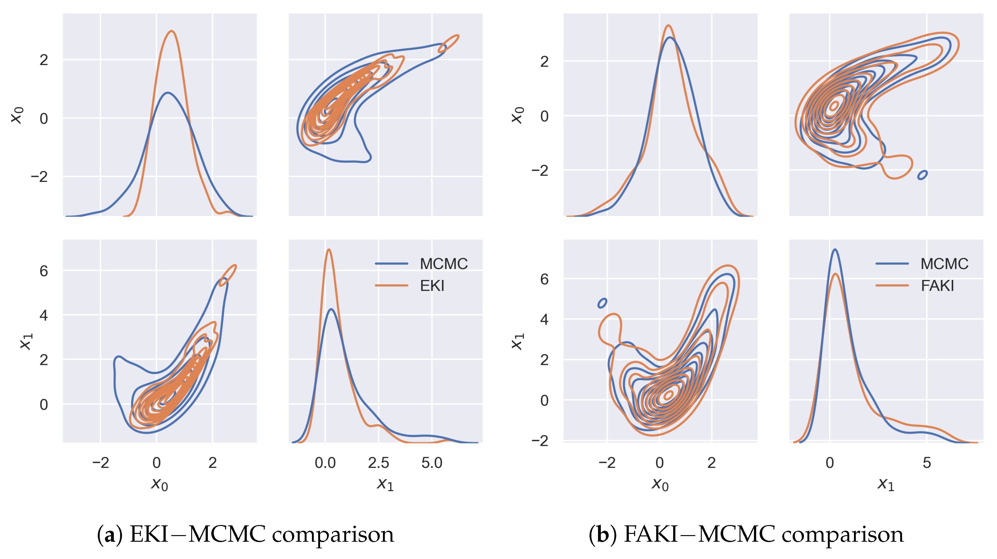
In Figure 1, we show pair plots comparing the final particle distributions obtained with EKI and FAKI against samples obtained through a long run of HMC. The NF mapping meant that the ensemble approximation obtained by FAKI was able to capture the highly non-linear target geometry. In comparison, EKI struggled to fill the tails of the Rosenbrock target. Moreover, whilst FAKI converged within ∼34 iterations, EKI required a median number of ∼100 iterations to converge using the ESS-based annealing scheme.
3.2. Stochastic Lorenz System
The Lorenz equations are a set of coupled differential equations used as a simple model of atmospheric convection. Notably, for certain parameter values, the Lorenz equations are known to exhibit chaotic behavior [24]. In this work, we followed [25] and considered the stochastic Lorenz system
where , , and are Gaussian white noise processes with standard deviation . To generate simulated, data we integrated these equations using a Euler–Maruyama scheme with for 30 steps, with initial conditions . The observations were then taken to be the values over these 30 time steps, with Gaussian observational noise .
The goal of our inference here was to recover the initial conditions, the trajectories and the innovation noise scale , giving a parameter space of dimensions. We assigned priors over these parameters as
where , , and are the transition functions corresponding to Equations (17)–(19), respectively. The Gaussian likelihood has the form
where are the observations of the trajectory. The chaotic dynamics of the Lorenz system resulted in a highly non-Gaussian prior distribution, with the inversion having to proceed through a sequence of highly non-Gaussian intermediate measures towards the posterior. This severely frustrated the performance of EKI, with the Gaussian ansatz failing to describe the geometry of the intermediate measures. For each run of EKI and FAKI, we used 940 particles.
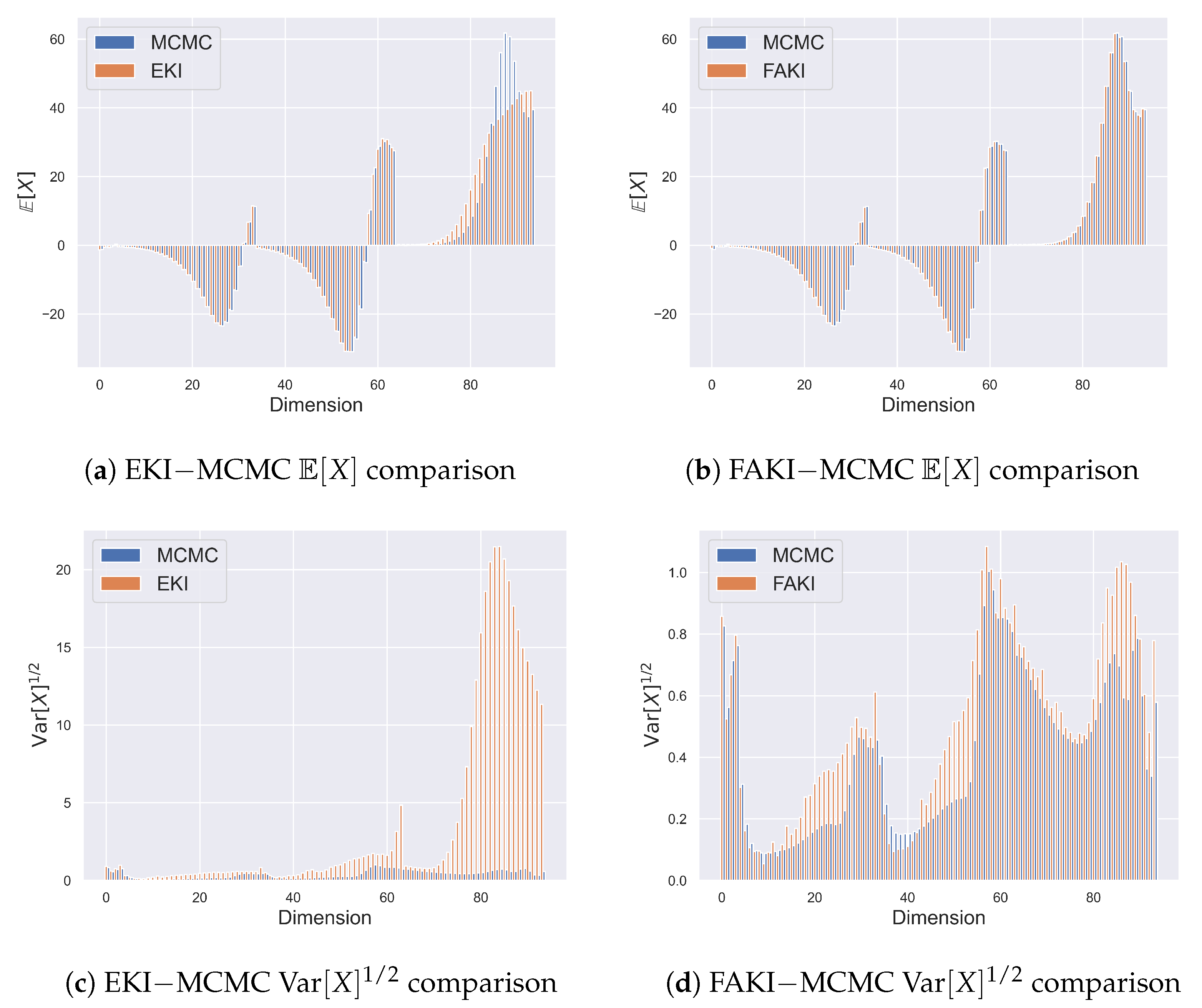
In Figure 2, we show the ensemble estimates for the mean and standard deviation along each dimension obtained by EKI and FAKI, compared to reference estimates obtained through long runs of HMC. FAKI was able to obtain accurate mean estimates along each dimension, whereas EKI was unable to obtain the correct means for much of the trajectory. EKI severely overestimated the marginal standard deviations along many dimensions. This situation was alleviated by the NF mappings learned by FAKI. The greater fidelity of the FAKI posterior approximations is reflected in the median estimates for the 1-Wasserstein distances, with a value of for FAKI and for EKI.
4. Conclusions
In this work, we introduced Flow Annealed Kalman Inversion (FAKI), a gradient-free inference algorithm for Bayesian inverse problems with expensive forward models. This is a generalization of Ensemble Kalman Inversion (EKI) where we utilize normalizing flows (NFs) to replace the Gaussian ansatz made in EKI. Instead of constructing a sequence of ensemble approximations to Gaussian measures that approximate a sequence of intermediate measures, as we move from the prior to the posterior, we learn an NF mapping at each iteration to a Gaussian latent space. Provided the transition between temperature levels is controlled, we can perform Kalman inversion updates in the NF latent space. In the NF latent space, the Gaussianity assumptions of EKI are more closely satisfied, resulting in a more stable inversion at each temperature level.
We demonstrated the performance of FAKI on two numerical benchmarks, a Rosenbrock distribution and a stochastic Lorenz system. Both examples exhibited significant non-Gaussianity in the transition from prior to posterior that frustrated standard EKI. In the presence of strong non-Gaussianity, we found that FAKI produced higher-fidelity posterior approximations compared to EKI, as measured by the 1-Wasserstein distance between FAKI/EKI samples and reference HMC samples. In addition to the improved fidelity of the posterior approximations, we found that FAKI tended to reduce the number of iterations required for convergence.
Whilst the application of NFs is able to relax the Gaussian ansatz of EKI, it does not address the linearity assumptions used in deriving EKI. As such, FAKI is still not exact for general forward models. In future work, it will be interesting to explore methods to address this: for example, the combination of FAKI with unbiased MCMC or importance sampling methods. It would also be interesting to consider generalizations of FAKI that are able to accommodate non-Gaussian likelihoods and/or parameter-dependent noise covariances. The use of NFs means that we typically require ensemble sizes to learn accurate NF maps with the MAF architecture employed in this work. It would be useful to explore alternative NF architectures and regularization schemes that are able to learn accurate NF maps with smaller ensemble sizes, in order to enable FAKI to scale to higher dimensions. In this work, we found that the MAF architecture is able to capture a wide range of target geometries without the need for expensive NF hyper-parameter searches. However, it may be possible to exploit NF architectures with inductive biases that are particularly suited to common target geometries, e.g., the non-linear correlations that often appear in hierarchical models.
Author Contributions
Conceptualization, U.S.; methodology, R.D.P.G. and U.S.; software, R.D.P.G. and M.K.; validation, R.D.P.G.; formal analysis, R.D.P.G.; investigation, R.D.P.G. and M.K.; resources, U.S.; data curation, R.D.P.G. and M.K.; writing—original draft preparation, R.D.P.G.; writing—review and editing, R.D.P.G., M.K. and U.S.; visualization, R.D.P.G.; supervision, U.S.; project administration, U.S.; funding acquisition, R.D.P.G. and U.S. All authors have read and agreed to the published version of the manuscript.
Funding
This research was funded by NSFC (grant No. 12250410240) and the U.S. Department of Energy, Office of Science, Office of Advanced Scientific Computing Research under Contract No. DE-AC02-05CH11231 at Lawrence Berkeley National Laboratory to enable research for Data-intensive Machine Learning and Analysis. RDPG was supported by a Tsinghua Shui Mu Fellowship.
Institutional Review Board Statement
Not applicable.
Informed Consent Statement
Not applicable.
Data Availability Statement
The code and data underlying this work can be made available upon contacting the corresponding author.
Acknowledgments
The authors thank Qijia Jiang and David Nabergoj for helpful discussions.
Conflicts of Interest
The authors declare no conflict of interest.
References
- Iglesias, M.A.; Law, K.J.; Stuart, A.M. Ensemble Kalman methods for inverse problems. Inverse Probl. 2013, 29, 045001. [Google Scholar] [CrossRef]
- Iglesias, M.A. A regularizing iterative ensemble Kalman method for PDE-constrained inverse problems. Inverse Probl. 2016, 32, 025002. [Google Scholar] [CrossRef]
- Schillings, C.; Stuart, A.M. Analysis of the ensemble Kalman filter for inverse problems. SIAM J. Numer. Anal. 2017, 55, 1264–1290. [Google Scholar] [CrossRef]
- Chada, N.K.; Iglesias, M.A.; Roininen, L.; Stuart, A.M. Parameterizations for ensemble Kalman inversion. Inverse Probl. 2018, 34, 055009. [Google Scholar] [CrossRef]
- Schillings, C.; Stuart, A.M. Convergence analysis of ensemble Kalman inversion: The linear, noisy case. Appl. Anal. 2018, 97, 107–123. [Google Scholar] [CrossRef]
- Iglesias, M.; Yang, Y. Adaptive regularisation for ensemble Kalman inversion. Inverse Probl. 2021, 37, 025008. [Google Scholar] [CrossRef]
- Huang, D.Z.; Schneider, T.; Stuart, A.M. Iterated Kalman methodology for inverse problems. J. Comput. Phys. 2022, 463, 111262. [Google Scholar] [CrossRef]
- Huang, D.Z.; Huang, J.; Reich, S.; Stuart, A.M. Efficient derivative-free Bayesian inference for large-scale inverse problems. Inverse Probl. 2022, 38, 125006. [Google Scholar] [CrossRef]
- Geyer, C.J. Practical Markov Chain Monte Carlo. Stat. Sci. 1992, 7, 473–483. [Google Scholar] [CrossRef]
- Gelman, A.; Gilks, W.R.; Roberts, G.O. Weak convergence and optimal scaling of random walk Metropolis algorithms. Ann. Appl. Probab. 1997, 7, 110–120. [Google Scholar] [CrossRef]
- Cotter, S.L.; Roberts, G.O.; Stuart, A.M.; White, D. MCMC Methods for Functions: Modifying Old Algorithms to Make Them Faster. Stat. Sci. 2013, 28, 424–446. [Google Scholar] [CrossRef]
- Del Moral, P.; Doucet, A.; Jasra, A. Sequential Monte Carlo Samplers. J. R. Stat. Soc. Ser. B Stat. Methodol. 2006, 68, 411–436. [Google Scholar] [CrossRef]
- Evensen, G. Sequential data assimilation with a nonlinear quasi-geostrophic model using Monte Carlo methods to forecast error statistics. J. Geophys. Res. Ocean. 1994, 99, 10143–10162. [Google Scholar] [CrossRef]
- Xiao, H.; Wu, J.L.; Wang, J.X.; Sun, R.; Roy, C. Quantifying and reducing model-form uncertainties in Reynolds-averaged Navier–Stokes simulations: A data-driven, physics-informed Bayesian approach. J. Comput. Phys. 2016, 324, 115–136. [Google Scholar] [CrossRef]
- Schneider, T.; Lan, S.; Stuart, A.; Teixeira, J. Earth system modeling 2.0: A blueprint for models that learn from observations and targeted high-resolution simulations. Geophys. Res. Lett. 2017, 44, 12–396. [Google Scholar] [CrossRef]
- Kovachki, N.B.; Stuart, A.M. Ensemble Kalman inversion: A derivative-free technique for machine learning tasks. Inverse Probl. 2019, 35, 095005. [Google Scholar] [CrossRef]
- Dinh, L.; Sohl-Dickstein, J.; Bengio, S. Density estimation using Real NVP. In Proceedings of the 5th International Conference on Learning Representations, ICLR 2017, Toulon, France, 24–26 April 2017; Conference Track Proceedings. Available online: https://openreview.net/ (accessed on 30 June 2023).
- Papamakarios, G.; Murray, I.; Pavlakou, T. Masked Autoregressive Flow for Density Estimation. In Proceedings of the Advances in Neural Information Processing Systems 30: Annual Conference on Neural Information Processing Systems 2017, Long Beach, CA, USA, 4–9 December 2017; Guyon, I., von Luxburg, U., Bengio, S., Wallach, H.M., Fergus, R., Vishwanathan, S.V.N., Garnett, R., Eds.; Neural Information Processing Systems Foundation, Inc. (NeurIPS): La Jolla, CA, USA, 2017; pp. 2338–2347. [Google Scholar]
- Kingma, D.P.; Dhariwal, P. Glow: Generative Flow with Invertible 1x1 Convolutions. In Proceedings of the Advances in Neural Information Processing Systems 31: Annual Conference on Neural Information Processing Systems 2018, NeurIPS 2018, Montréal, QC, Canada, 3–8 December 2018; Bengio, S., Wallach, H.M., Larochelle, H., Grauman, K., Cesa-Bianchi, N., Garnett, R., Eds.; NeurIPS: La Jolla, CA, USA, 2018; pp. 10236–10245. [Google Scholar]
- Dai, B.; Seljak, U. Sliced Iterative Normalizing Flows. In Proceedings of the 38th International Conference on Machine Learning, ICML 2021, Virtual Event, 18–24 July 2021; Meila, M., Zhang, T., Eds.; Proceedings of Machine Learning Research. PMLR: New York, NY, USA, 2021; Volume 139, pp. 2352–2364. [Google Scholar]
- De Simon, L.; Iglesias, M.; Jones, B.; Wood, C. Quantifying uncertainty in thermophysical properties of walls by means of Bayesian inversion. Energy Build. 2018, 177, 220–245. [Google Scholar] [CrossRef]
- Iglesias, M.; Park, M.; Tretyakov, M. Bayesian inversion in resin transfer molding. Inverse Probl. 2018, 34, 105002. [Google Scholar] [CrossRef]
- Karamanis, M.; Beutler, F.; Peacock, J.A.; Nabergoj, D.; Seljak, U. Accelerating astronomical and cosmological inference with preconditioned Monte Carlo. Mon. Not. R. Astron. Soc. 2022, 516, 1644–1653. [Google Scholar] [CrossRef]
- Lorenz, E.N. Deterministic Nonperiodic Flow. J. Atmos. Sci. 1963, 20, 130–148. [Google Scholar] [CrossRef]
- Ambrogioni, L.; Lin, K.; Fertig, E.; Vikram, S.; Hinne, M.; Moore, D.; van Gerven, M. Automatic structured variational inference. In Proceedings of the International Conference on Artificial Intelligence and Statistics, Virtual, 13–15 April 2021; PMLR: New York, NY, USA, 2021; pp. 676–684. [Google Scholar]
- Villani, C. Optimal Transport—Old and New; Springer: Berlin/Heidelberg, Germany, 2008; Volume 338, pp. xxii+973. [Google Scholar]
- Zhang, L.; Carpenter, B.; Gelman, A.; Vehtari, A. Pathfinder: Parallel quasi-Newton variational inference. J. Mach. Learn. Res. 2022, 23, 13802–13850. [Google Scholar]
- Neal, R.M. MCMC using Hamiltonian dynamics. Handb. Markov Chain. Monte Carlo 2011, 2, 2. [Google Scholar]
- Hoffman, M.D.; Gelman, A. The No-U-Turn sampler: Adaptively setting path lengths in Hamiltonian Monte Carlo. J. Mach. Learn. Res. 2014, 15, 1593–1623. [Google Scholar]
Figure 1.
Pair plots for the Rosenbrock target. Panel (a): pair-plot comparison of samples from EKI and a long HMC run. Panel (b): pair-plot comparison of samples from FAKI and a long HMC run. Samples from FAKI were able to correctly capture the highly non-linear target geometry. Standard EKI struggled to fill the tails of the target and required ∼100 iterations to converge, compared to ∼34 iterations for FAKI.

Figure 2.
Comparison of first and second moment estimates along each dimension for the stochastic Lorenz system. Panel (a): comparison between the mean estimates from EKI and a long HMC run. Panel (b): comparison between the mean estimates from FAKI and a long HMC run. Panel (c): comparison between the standard deviation estimates from EKI and a long HMC run. Panel (d): comparison between the standard deviation estimates from FAKI and a long HMC run. Blue bars indicate the moment estimates obtained via HMC along each dimension, with the adjacent orange bars showing the estimates obtained through EKI/FAKI. EKI was unable to obtain accurate mean estimates for much of the trajectory, whilst FAKI was able to obtain accurate mean estimates for each dimension. FAKI outperformed EKI in its estimates of the marginal standard deviations, with EKI drastically overestimating the standard deviations along many dimensions.


Table 1.
Median and MAD values of and 1-Wasserstein distances for each model and algorithm combination, calculated over 10 independent runs using different random seeds. For both numerical benchmarks, we see that FAKI resulted in a reduced number of iterations for convergence and a lower value of the 1-Wasserstein distance between the converged samples and the ground truth.
| Model | Algorithm | ||||
|---|---|---|---|---|---|
| Rosenbrock | EKI | 100 | 7.0 | 0.72 | 0.05 |
| Rosenbrock | FAKI | 34.0 | 7.0 | 0.43 | 0.14 |
| Lorenz | EKI | 10.0 | 0.0 | 69.8 | 1.08 |
| Lorenz | FAKI | 8.0 | 0.0 | 5.65 | 0.86 |
Disclaimer/Publisher’s Note: The statements, opinions and data contained in all publications are solely those of the individual author(s) and contributor(s) and not of MDPI and/or the editor(s). MDPI and/or the editor(s) disclaim responsibility for any injury to people or property resulting from any ideas, methods, instructions or products referred to in the content. |
© 2024 by the authors. Licensee MDPI, Basel, Switzerland. This article is an open access article distributed under the terms and conditions of the Creative Commons Attribution (CC BY) license (https://creativecommons.org/licenses/by/4.0/).
Share and Cite
MDPI and ACS Style
Grumitt, R.D.P.; Karamanis, M.; Seljak, U. Flow Annealed Kalman Inversion for Gradient-Free Inference in Bayesian Inverse Problems. Phys. Sci. Forum 2023, 9, 21. https://doi.org/10.3390/psf2023009021
AMA Style
Grumitt RDP, Karamanis M, Seljak U. Flow Annealed Kalman Inversion for Gradient-Free Inference in Bayesian Inverse Problems. Physical Sciences Forum. 2023; 9(1):21. https://doi.org/10.3390/psf2023009021
Chicago/Turabian StyleGrumitt, Richard D. P., Minas Karamanis, and Uroš Seljak. 2023. "Flow Annealed Kalman Inversion for Gradient-Free Inference in Bayesian Inverse Problems" Physical Sciences Forum 9, no. 1: 21. https://doi.org/10.3390/psf2023009021