
SEIR Modeling, Simulation, Parameter Estimation, and Their Application for COVID-19 Epidemic Prediction †


1
Department of Mathematics, University of Mazandran, Babolsar 47415-95447, Iran
2
International Science Consulting and Training (ISCT), 91440 Bures sur Yvette, France
3
Scientific Leader of Shanfeng Blower Company, Shangyu District, Shaoxing 312300, China
*
Author to whom correspondence should be addressed.
†
Presented at the 41st International Workshop on Bayesian Inference and Maximum Entropy Methods in Science and Engineering, Paris, France, 18–22 July 2022.
Phys. Sci. Forum 2022, 5(1), 18; https://doi.org/10.3390/psf2022005018
Published: 5 December 2022
(This article belongs to the Proceedings of The 41st International Workshop on Bayesian Inference and Maximum Entropy Methods in Science and Engineering)
Abstract
:In this paper, we consider the SEIR (Susceptible-Exposed-Infectious-Removed) model for studying COVID-19. The main contributions of this paper are: (i) a detailed explanation of the SEIR model, with the significance of its parameters. (ii) calibration and estimation of the parameters of the model using the observed data. To do this, we used a nonlinear least squares (NLS) optimization and a Bayesian estimation method. (iii) When the parameters are estimated, we use the models for the prediction of the spread of the virus and compute the probable number of infections and deaths of individuals. (iii) We show the performances of the proposed method on simulated and real data. (iv) Remarking that the fixed parameter model could not give satisfactory results on real data, we proposed the use of a time-dependent parameter model. Then, this model is implemented and used on real data.
1. Introduction
Mathematical models and computer simulations are useful experimental tools for building and testing theories, assessing quantitative conjectures, determining sensitivities to changes in parameter values, and estimating key parameters from data. Understanding the transmission characteristics of infectious diseases in communities, regions, and countries can lead to better approaches to controlling the transmission of those diseases. Mathematical models are utilized in comparing, planning, implementing, evaluating, and optimizing numerous detection, prevention, therapy, and management programs. Epidemiology modeling can contribute to the design and analysis of epidemiological surveys, recommend crucial data that should be collected, determine trends, make general forecasts, and estimate the uncertainty in forecasts [1,2,3,4].
There exist a number of models for infectious diseases; as for compartmental models, starting from the very classical SIR model to additional complicated proposals [5]. Many research works have been reported. They show that those SIS, SIR and SEIR models can replicate the dynamics of various epidemics. These models have also been used to model COVID-19 [6,7,8]. To mention a few of them, Tang et al. [9] investigated a general SEIR epidemiological model where quarantine, isolation, and treatment are considered. Wang et al. [10] applied the phase-adjusted estimation for the amount of COVID-2019 cases in Wuhan.
Our main contribution is to consider the SEIR compartmented model and to give the significance of its parameters; methods for the estimation of its parameters and its calibration, and finally, use it for prediction. For the estimation of its parameter, we used two methods: a deterministic nonlinear least squares (NLS) optimization and a Bayesian estimation method. Once the parameters are estimated, we use the model for the prediction of the spread of the virus and calculate the probable number of infections and deaths of individuals. We show the performances of the proposed method on simulated data. Remarking that the fixed-parameter model could not provide satisfactory results on real data, we proposed the use of a time-dependent parameter model.
The rest of this paper is organized as follows. Section 2 describes the construction of the mathematical SEIR model and the comprehension of its parameters. Section 3 focuses on the estimation of the parameters of SEIR using simulated data. In Section 4, the focus is on the application of this model for the available data. We will see how to adapt the parameter estimation to the available data. Remarking that the evolution of the COVID-19 epidemy can not be modeled by a fixed-parameter model, we adopt a time-varying parameter model and adapt it to the available data. In Section 5, we describe the main conclusions.
2. A Continuous-Time SEIR Models
SEIR is a classical model for the problem of modeling epidemics. This model is composed of four components, shown in Figure 1.
The dynamic equations relating these compartments are given by:
In this model:
- Susceptible is the variety of people susceptible to contracting the infection;
- Exposed the variety of individuals exposed who are alive but not infected;
- Infectious is the variety of individuals that are infected;
- Recovered is the cumulative variety of individuals that recovered from the disease.
The total population at time t is represented by The significance of the parameters are: is the infection rate or the speed of spread, is the incubation rate or the rate of latent individuals becoming infectious (average period of incubation is ), and is the recovery rate or mortality rate. If the duration of infection is D then This model has the initial conditions , and . Note that
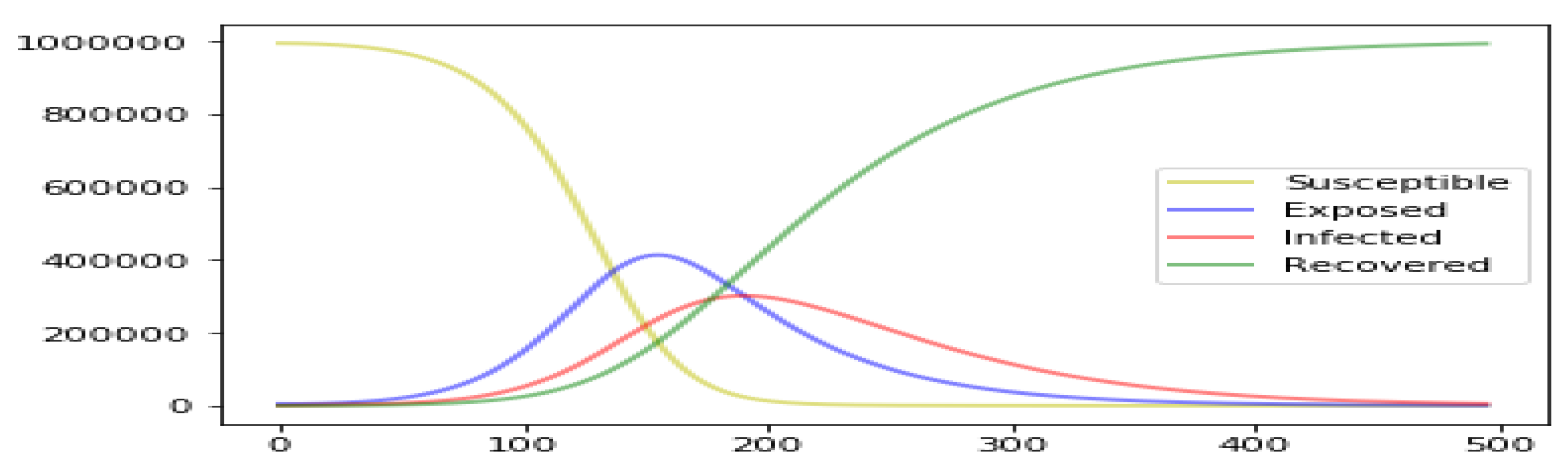
Figure 2 shows an example simulation of this model.
3. Calibration of the Epidemic Model
With such a set of differential equations, the mathematical problems to solve are mainly in two categories: forward and inverse problems. The forward problem consists of computing the outputs when the parameters and the initial conditions are fixed. The inverse problems consist of: (i) estimating the parameters when a set of observable data related to the outputs are given; (ii) predict unobserved parts of outputs (future values) from the observed (passed data) when the parameters are estimated. Let us first explain these in a more formal and general mathematical formulation.
3.1. Forward Problem
Consider now the following general SEIR
in which
- is the 4-dimensional state vector;
- the initial state is a constant 4-dimensional vector;
- is the 3-dimensional vector of the model parameters;
- is a continuous map, which is described on the open set
The forward problem consists in computing the model response given the initial conditions and a set of parameters .
3.2. Inverse Problem
The inverse problem is the opposite of the forward problem: Given a set of observed data , we try to estimate parameter , and then, the state vector for all t, and thus, the unobserved values of (prediction). There are mainly two approaches to inverse problems: deterministic and probabilistic. In the following, we describe these two approaches through two methods: i) the nonlinear least squares (NLS) and the Bayesian maximum a posteriori (MAP).
3.3. Nonlinear Least Squares (NLS) Solution
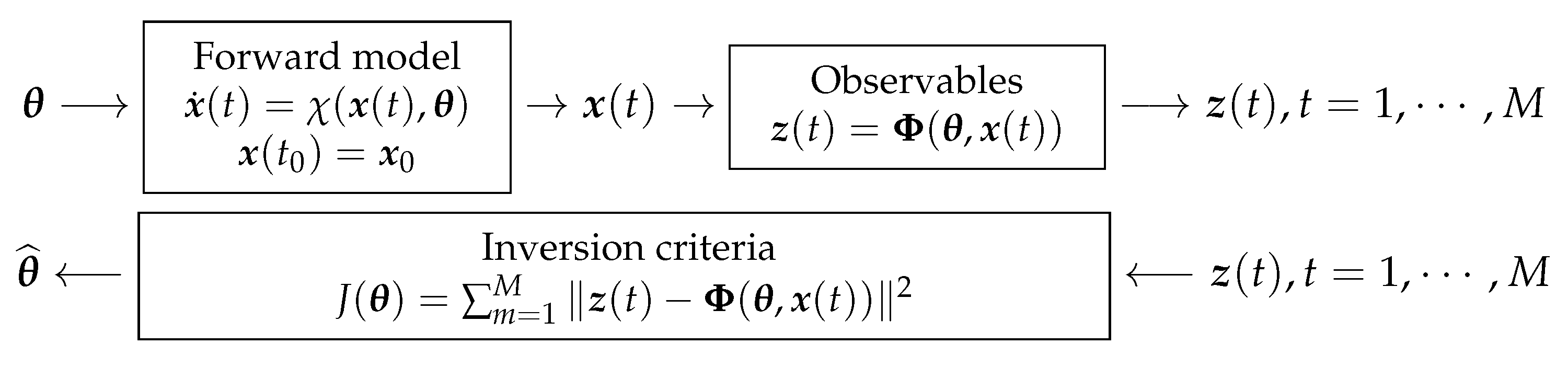
Figure 3 schematically shows the forward and inverse problems in a deterministic approach.
The nonlinear least squares method (NLS) is used numerically to approximate a solution for the inverse problem (3) within the least-squares fitting, where we look for the value of the model parameter , which minimizes the least squares criterion
where is the output of the model for a given set of parameters and is the observable outputs.
Such a problem is clearly a nonlinear least-squares problem, since the dependence of a solution system on the parameter is through a highly nonlinear system of differential equations.
3.4. Bayesian Estimation Framework
In a Bayesian framework, first, we may consider Equation (4) as the log-likelihood of parameters in the data:
This means that we assume that there is some uncertainty on the observed data and that the only thing we know about those errors is that they are centered (zero mean), identically and independently distributed with fixed variance . In fact, this formal prior knowledge is translated by the maximum entropy principle (MEP) to a Gaussian distribution [11].
We may then assign or choose a prior to translate any prior knowledge we may have about . This can be just flat priors on the parameters or, rather, some reference, noninformative, or conjugate priors. In this work, as all the parameters are the rates (infection rate, incubation rate, and recovery rate), we used flat priors for them.
When the likelihood and the prior are fixed, we can use the Bayesian rule to obtain the posterior law:
from which we can infer . If we choose the maximum a posteriori (MAP) solution
we arrive at
where with is given by (4), and is a hyperparameter depending on the variance of the errors and some parameters of the prior law.
Comparing the expressions in (4) and (8), we see that the MAP solution can be considered as a regularized solution to the standard NLS solution with as the regularization parameter. In our case, as we have chosen flat priors, , and so the criterion to optimize (8) becomes the same as criterion (4).
There are many other Bayesian estimators, for example, the posterior mean, but its inference needs MCMC sampling methods. The computational cost of such methods is huge for this kind of application. We stand here with the more classical techniques of Chi-squared, AIC (Akaike Information Criterion), and BIC (Bayesian Information Criterion) for which standard techniques of computations are, in general, included in many optimization tools available, for example, in Python language packages [12]. A Jupyter notebook of all the simulations of this paper will be available after its publication on github.
3.5. Adaptation of the Inversion Methods to Available Data
Now we confront the modeling of the previous section with accessible data that can not be a whole time series but a subset or alternative combination of them. As we work with the COVID-19 data from the Johns Hopkins University at GitHub [13], the available data are:
- Confirmed (C)
- Dead (D)
- Recovered (R)
as cumulative integer-valued time series for days from 22 January 2020. Note that these values are absolute numbers, not relative to a total population. Note that the unconfirmed cases and also the Susceptibles are not accessible at all, whereas the Confirmed contain the Dead and the Recovered from earlier days. For example, using the Johns Hopkins data, they supply C, D, and R individually while not stating the most necessary variables . We currently use a model that works with the Johns Hopkins data while not having the ability to use S in the SEIR model. Since the SEIR model does not distinguish between recoveries and deaths, we set the following relations:
Now, returning to the SEIR model, we see the subsequent relations:
defining time series and that model and without knowing SEIR. This is equivalent to the model
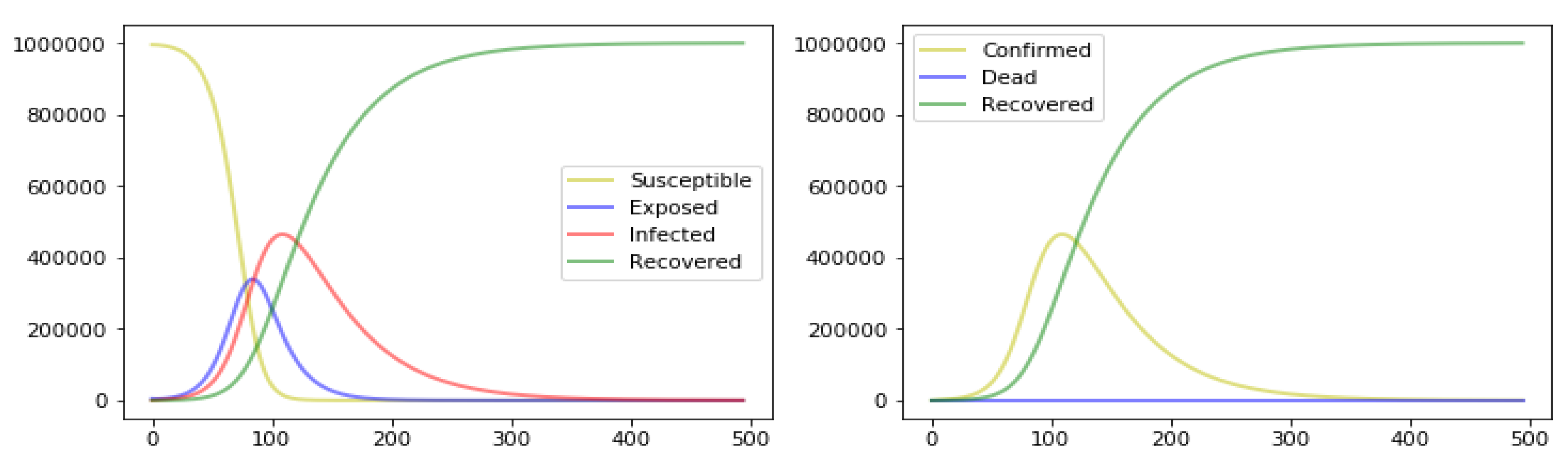
Then, for the estimation of the parameters with its adaptation Figure 4 indicates the conversion from S-E-I-R to C-D-R.
This straightforward model has at least two drawbacks:
- It assumes that the number of the population N does not change during the epidemic;
- It does not account for possible context modification of the sickness (fixed parameters during the whole analysis).
Numerous extensions are supplied to enhance it. The primary extension of the model with a further block is utilized to account for the specific fact that the whole number of the population is not fixed [7,14,15,16,17,18,19,20,21,22]. The second categories propose time-dependent parameters [23,24,25,26].
4. Constructing Predictions
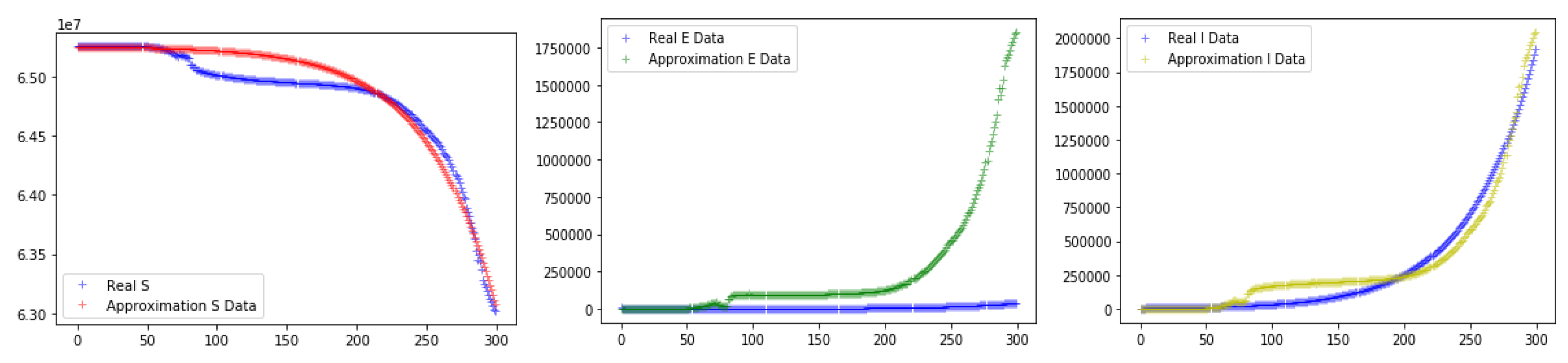
To use the proposed model to perform prediction, the process we propose is, first estimate the parameters of the model from the real available data using the method presented in Figure 5 using either the nonlinear least squares or Bayesian methods. Then, once the model has been identified from the data, we can use it for prediction. To be more precise, we first consider that we have real data over the horizon where 1 denotes the first day of the estimation period and T the last one. We can initialize the state of the system with from the real data. Then, with an initial value for the parameters, we can compute , then and finally the value of criterion , which can then be iteratively optimized to obtain the final estimation of the parameters. When the parameters are obtained, we can use them to perform any prediction of state and then for any time interval, particularly for any
Analysis of COVID-19 Data for France
Daily overall incidences of COVID-19 cases were collected from information sources on github. The records showed the simplest date of the first positive Corona test, date of release from hospital, and typically, date of first negative Corona test. Cases that did not arise via transmission started at ; and cases that arose via transmission were marked on the day of the first positive Corona test. The optimal parameter values obtained using the procedure given in Section 3.3 are In Figure 5, we present the results of simulations of the variety of S, I, and R listed through time for France with a fixed-parameter model.
However, the fixed-parameter model could not give satisfactory results on real data, so we used a time-dependent parameter model. Specifically, a straightforward periodic function :
Parameter a denotes the baseline or average transmission rate, is the period of the forcing, and b represents the amplitude of the disease.
5. Conclusions and Discussion
The SEIR model we used here appears to be useful for understanding the propagation of the virus. Two main difficulties appeared:
- First, the available data (C,D,R) could not determine in a unique way the S,E,I,R. In fact, going from (S,E,I,R) to (C,D,R) is unique, but the inverse is not. Therefore, we had to be careful when directly using the original SEIR model. We explained this in the previous section when we wanted to estimate the parameters of the model from the real (C,D,R) data.
- The second difficulty appeared when we saw that the fixed parameters model could not predict the real data well. This is explained due to the fact that this simple model does not account for many real situations. In particular, a fixed-parameter model does not correspond to reality. Many works have been performed to overcome these difficulties. Between them, we chose a simple method in which parameter varies over time. We used a periodic time dependent for this parameter, as it was also used by other researchers [23,24,25,26]. Finally, using appropriate values for the parameters a and b of this time-dependent model, we could obtain good predictions with real data.
Author Contributions
Conceptualization, E.T. and A.M.-D.; methodology, E.T. and A.M.-D.; software, E.T. and A.M.-D.; validation, A.M.-D.; formal analysis, E.T. and A.M.-D.; investigation, E.T. and A.M.-D.; resources, E.T. and A.M.-D.; data curation, E.T.; writing—original draft preparation, E.T.; writing—review and editing, A.M.-D.; visualization, E.T. and A.M.-D.; supervision, A.M.-D.; project administration, A.M.-D.; funding acquisition, A.M.-D. All authors have read and agreed to the published version of the manuscript.
Funding
This research received no external funding.
Institutional Review Board Statement
Not applicable.
Informed Consent Statement
Not applicable.
Data Availability Statement
The presented data is available at https://github.com/CSSEGISandData/COVID-19.
Conflicts of Interest
The authors declare no conflict of interest.
References
- Hethcote, H.W. The mathematics of infectious diseases. SIAM Rev. 2000, 42, 599–653. [Google Scholar] [CrossRef] [Green Version]
- Vynnycky, E.; White, R. An Introduction to Infectious Disease Modelling; Oxford University Press: Oxford, UK, 2010. [Google Scholar]
- Stefan Ma, Y.X. Mathematical Understanding of Infectious Disease Dynamics; World Scientific: Singapore, 2008. [Google Scholar]
- Larremore, D.B.; Fosdick, B.K.; Bubar, K.M.; Zhang, S.; Kissler, S.M.; Metcalf, C.J.E.; Buckee, C.O.; Grad, Y.H. Estimating SARS-CoV-2 seroprevalence and epidemiological parameters with uncertainty from serological surveys. Elife 2021, 10. [Google Scholar] [CrossRef] [PubMed]
- Brauer, F.; Castillo-Chavez, C.; Feng, Z. Mathematical Models in Epidemiology; Springer: New York, NY, USA, 2019. [Google Scholar]
- Paulo, R.; Zingano, J.P.Z. A matlab code to compute reproduction numbers with applications to the Covid-19 outbreak. arXiv 2020, arXiv:2006.13752. [Google Scholar]
- He, S.; Peng, Y.; Sun, K. SEIR modeling of the COVID-19 and its dynamics. Nonlinear Dyn. 2020, 101, 1667–1680. [Google Scholar] [CrossRef] [PubMed]
- Gleeson, J.P.; Murphy, T.B.; O’Brien, J.D.; O’Sullivan, D.J. A Population-Level SEIR Model for COVID-19 Scenarios. In Technical Note of the Irish Epidemiological Modelling Advisory Group to NPHET; Department of Health, Government of Ireland: Dublin, Ireland, 2020. [Google Scholar]
- Tang, Z.; Li, X.; Li, H. Prediction of New Coronavirus Infection Based on a Modified SEIR Model. medRxiv 2020. [Google Scholar] [CrossRef]
- Yang, Z.; Zeng, Z.; Wang, K.; Wong, S.S.; Liang, W.; Zanin, M.; Liu, P.; Cao, X.; Gao, Z.; Mai, Z.; et al. Modified SEIR and AI prediction of the epidemics trend of COVID-19 in China under public health interventions. J. Thorac. Dis. 2020, 12, 867–874. [Google Scholar] [CrossRef] [PubMed]
- Muñoz-Cobo, J.L.; Mendizábal, R.; Miquel, A.; Berna, C.; Escrivá, A. Use of the Principles of Maximum Entropy and Maximum Relative Entropy for the Determination of Uncertain Parameter Distributions in Engineering Applications. Entropy 2017, 48, 486. [Google Scholar] [CrossRef] [Green Version]
- Yang, X.S. Introduction to Algorithms for Data Mining and Machine Learning; Academic Press: Cambridge, MA, USA, 2019. [Google Scholar]
- Covid-19 Repository at Github. 2019. Available online: https://github.com/CSSEGISandData/COVID-19 (accessed on 22 January 2022).
- Aleta, A.; Martin-Corral, D.; y Piontti, A.P.; Ajelli, M.; Litvinova, M.; Chinazzi, M.; Dean, N.E.; Halloran, M.E.; Longini, I.M., Jr.; Merler, S.; et al. Modelling the impact of testing, contact tracing and household quarantine on second waves of COVID-19. Nat. Human Behav. 2020, 4, 964–971. [Google Scholar] [CrossRef]
- Grimm, V.; Mengel, F.; Schmidt, M. Extensions of the SEIR model for the analysis of tailored social distancing and tracing approaches to cope with COVID-19. Sci. Rep. 2021, 11, 1–16. [Google Scholar] [CrossRef]
- Byrne, A.W.; McEvoy, D.; Collins, A.; Hunt, K.; Casey, M.; Barber, A.; Butler, F.; Griffin, J.; Lane, E.; McAloon, C.; et al. Inferred duration of infectious period of SARS-CoV-2: Rapid scoping review and analysis of available evidence for asymptomatic and symptomatic COVID-19 cases. BMJ Open 2020, 10, e039856. [Google Scholar] [CrossRef] [PubMed]
- Kucharski, A.J.; Russell, T.W.; Diamond, C.; Liu, Y.; Edmunds, J.; Funk, S.; Eggo, R.M.; Sun, F.; Jit, M.; Munday, J.D.; et al. Early dynamics of transmission and control of COVID-19: A mathematical modelling study. Lancet Infect. D 2020, 20, 553–558. [Google Scholar] [CrossRef] [PubMed]
- Goswami, G.; Prasad, J.; Dhuria, M. Extracting the effective contact rate of COVID-19 pandemic. arXiv 2020, arXiv:2004.07750. [Google Scholar]
- Comunian, A.; Gaburro, R.; Giudici, M. Inversion of a SIR-based model: A critical analysis about the application to COVID-19 epidemic. Phys. D Nonlinear Phenom. 2020, 413, 132674. [Google Scholar] [CrossRef] [PubMed]
- Hunter, E.; Mac Namee, B.; Kelleher, J. A Hybrid Agent-Based and Equation Based Model for the Spread of Infectious Diseases. J. Artif. Soc. Soc. Simul. 2020, 23, 14. [Google Scholar] [CrossRef]
- Gleeson, J.P.; Murphy, T.B.; O’Brien, J.D.; O’Sullivan, D.J. A population-level SEIR model for COVID-19 scenarios (updated). In Technical Note of the Irish Epidemiological Modelling Advisory Group to NPHET; Department of Health, Government of Ireland: Dublin, Ireland, 2021. [Google Scholar]
- Prem, K.; Liu, Y.; Russell, T.W.; Kucharski, A.J.; Eggo, R.M.; Davies, N.; Flasche, S.; Clifford, S.; Pearson, C.A.; Munday, J.D.; et al. The effect of control strategies to reduce social mixing on outcomes of the COVID-19 epidemic in Wuhan, China: A modelling study. Lancet Public Health 2020, 5, e261–e270. [Google Scholar] [CrossRef] [PubMed] [Green Version]
- Mummert, A. Studying the recovery procedure for the time-dependent transmission rate(s) in epidemic models. J. Math. Biol. 2013, 67, 483–507. [Google Scholar] [CrossRef] [PubMed]
- Griffin, J.M.; Collins, A.; Hunt, K.; McEvoy, D.; Casey, M.; Byrne, A.; McAloon, C.G.; Barber, A.; Lane, E.; McEvoy, D.; et al. A rapid review of available evidence on the serial interval and generation time of COVID-19. medRxiv 2020. [Google Scholar] [CrossRef] [PubMed]
- Araujo, M.B.; Naimi, B. Spread of SARS-CoV-2 Coronavirus likely to be constrained by climate. medRxiv 2020. [Google Scholar] [CrossRef] [Green Version]
- Breton, T.R. The Effect of Temperature on the Spread of the Coronavirus in the U.S. SSRN 2020. [Google Scholar] [CrossRef]
Figure 1.
The four components of the SEIR model and their relations.

Figure 2.
A typical SEIR Model simulated solution. This result is obtained with the following parameters: , and the initial values: .
Figure 2.
A typical SEIR Model simulated solution. This result is obtained with the following parameters: , and the initial values: .

Figure 3.
Forward and inverse problems. Here, we assume that the initial conditions are known.

Figure 4.
Conversion from S-E-I-R to C-D-R.

Figure 5.
Prediction results with the SEIR model (time-varying parameter).

Figure 6.
Prediction results with the SEIR model (constant parameters).

Figure 7.
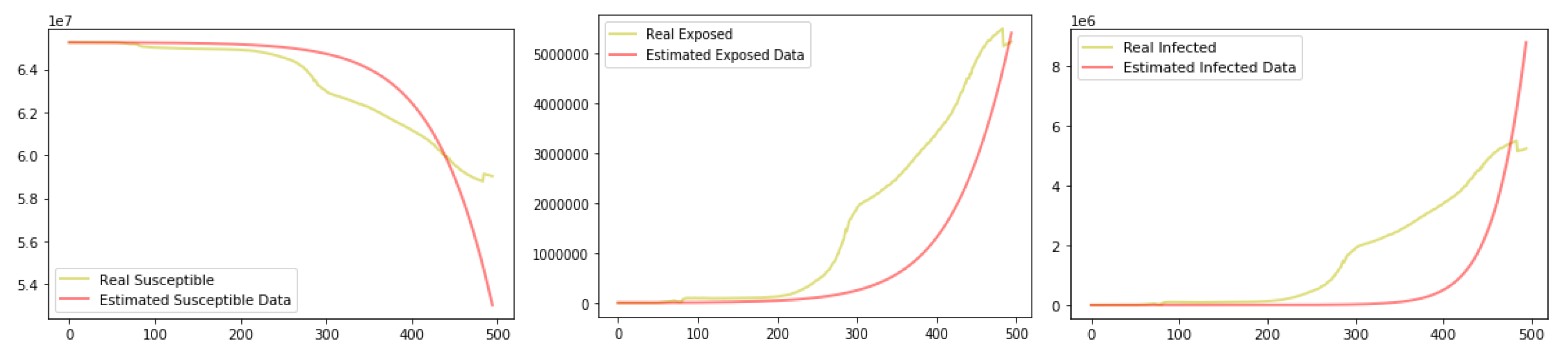
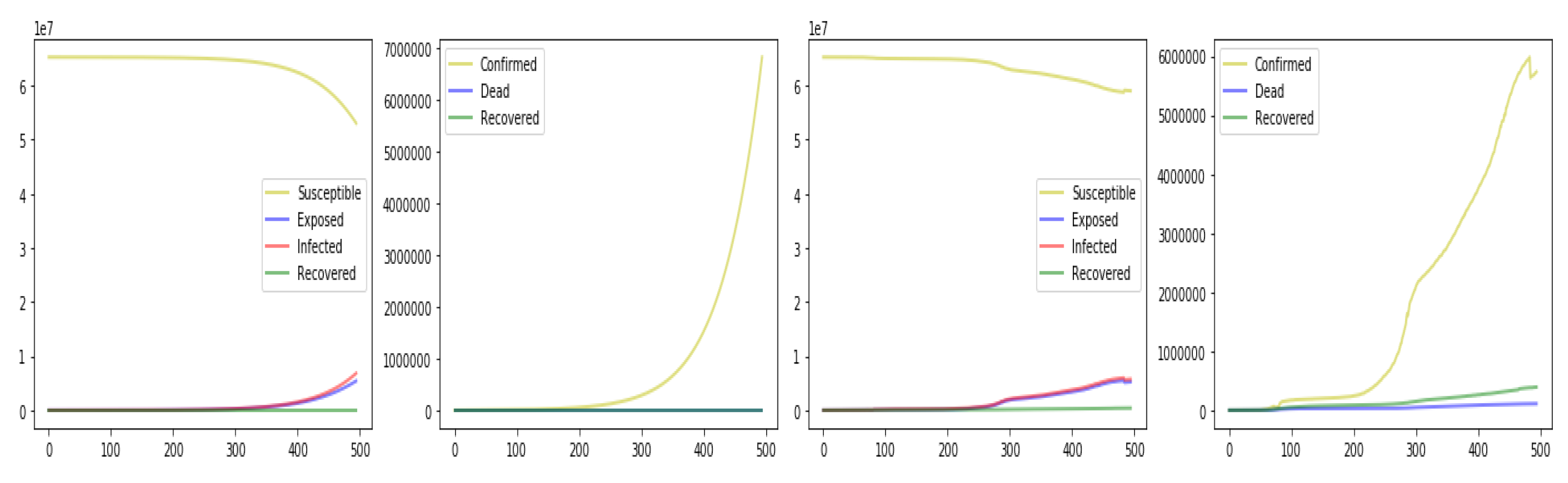
Left: Conversion from estimated S-E-I-R to C-D-R (time-varying parameter). Right: Conversion from S-E-I-R to C-D-R on real data.
Figure 7.
Left: Conversion from estimated S-E-I-R to C-D-R (time-varying parameter). Right: Conversion from S-E-I-R to C-D-R on real data.

Publisher’s Note: MDPI stays neutral with regard to jurisdictional claims in published maps and institutional affiliations. |
© 2022 by the authors. Licensee MDPI, Basel, Switzerland. This article is an open access article distributed under the terms and conditions of the Creative Commons Attribution (CC BY) license (https://creativecommons.org/licenses/by/4.0/).
Share and Cite
MDPI and ACS Style
Taghizadeh, E.; Mohammad-Djafari, A. SEIR Modeling, Simulation, Parameter Estimation, and Their Application for COVID-19 Epidemic Prediction. Phys. Sci. Forum 2022, 5, 18. https://doi.org/10.3390/psf2022005018
AMA Style
Taghizadeh E, Mohammad-Djafari A. SEIR Modeling, Simulation, Parameter Estimation, and Their Application for COVID-19 Epidemic Prediction. Physical Sciences Forum. 2022; 5(1):18. https://doi.org/10.3390/psf2022005018
Chicago/Turabian StyleTaghizadeh, Elham, and Ali Mohammad-Djafari. 2022. "SEIR Modeling, Simulation, Parameter Estimation, and Their Application for COVID-19 Epidemic Prediction" Physical Sciences Forum 5, no. 1: 18. https://doi.org/10.3390/psf2022005018