
Towards a Standard Method for Estimating Fragmentation Rates in Emulsification Experiments

Department of Food Technology, Engineering and Nutrition, LTH at Lund University, 221 00 Lund, Sweden
Processes 2021, 9(12), 2242; https://doi.org/10.3390/pr9122242
Submission received: 10 November 2021
/
Revised: 2 December 2021
/
Accepted: 9 December 2021
/
Published: 13 December 2021
(This article belongs to the Section Particle Processes)
Abstract
:The fragmentation rate function connects the fundamental drop breakup process with the resulting drop size distribution and is central to understanding or modeling emulsification processes. There is a large interest in being able to reliably measure it from an emulsification experiment, both for generating data for validating theoretical fragmentation rate function suggestions and as a tool for studying emulsification processes. Consequently, several methods have been suggested for measuring fragmentation rates based on emulsion experiments. Typically, each study suggests a new method that is rarely used again. The lack of an agreement on a standard method has become a substantial challenge. This contribution critically and systematically analyses four influential suggestions of how to measure fragmentation rate in terms of validity, reliability, and sensitivity to method assumptions. The back-calculation method is identified as the most promising—high reliability and low sensitivity to assumption—whereas performing a non-linear regression on a parameterized model (as commonly suggested) is unsuitable due to its high sensitivity. The simplistic zero-order method is identified as an interesting supplemental tool that could be used for qualitative comparisons but not for quantification.
1. Introduction
Emulsification is an important unit operation in many applications of chemical engineering, e.g., in food, pharmaceutical, cosmetics, and petroleum processing. It is defined as the process where (at least) two liquid phases are dispersed into one another, forming a kinetically stable colloidal system [1]. From a fundamental colloidal perspective, emulsification can be described as a combination of the primary breakup of large drops [2,3,4,5], re-coalescence of insufficiently stabilized drops [6] and adsorption of surface-active material at the drop interface [7]. Turbulent emulsification—where drops are broken up by turbulent stresses and coalescence is driven by turbulent orthokinetic collisions—is of special interest, since it dominates emulsion formation in technically relevant processes such as high-pressure homogenizers and rotor-stator mixers [8].
Emulsification has been the focus of intense research, due both to its relevance in industrial applications and due to its fundamental interest in colloidal science. However, two fairly distinct ‘branches’ can be identified in the literature, based on where the primary interest lies. One branch consists of research mainly intended to learn how to design and control the resulting emulsion properties, e.g., how different emulsifiers help form, stabilize and break emulsions, and what surface properties these systems obtain [1,7,9,10,11], or how different technically relevant emulsification conditions influence efficiencies [12,13,14,15]. This will be referred to as the applied branch of emulsification research.
The other branch consists of researchers mainly interesting in linking the breakup and coalescence taking place in emulsification devices to the first principle, i.e., describe how the breakup of a drop entering a turbulent field could be modeled mathematically in terms of conservation of mass, energy, and momentum [16,17,18,19,20,21,22,23,24]. Researchers working in this branch often have a mechanical engineering, or fluid mechanics background. This will be referred to as the fundamental branch of emulsification research in this contribution.
Whereas both branches work experimentally to understand emulsification, the focus of these experiments differ. Applied branch research often (but not exclusively) characterizes emulsification in terms of average drop size or drop size distributions (DSDs), frequently by using laser diffraction [25]. Researchers in the fundamental branch are more interested in measuring characteristic time scales or the rate at which drops break in a turbulent field, e.g., through idealized numerical experiments [21,26] or high-speed photography in idealized systems [27,28,29,30,31].
Substantial research effort in the fundamental branch has been spent on deriving theoretical fragmentation rate models. There is of yet no general agreement on which model is the most suitable; several comprehensive reviews of fragmentation rate models are available [18,32,33,34], and new theoretical models are suggested continuously [35,36].
The population balance equation (PBE) forms a natural link between the DSD (of main focus in the applied branch) and the fragmentation process (of main focus in the fundamental branch). When the volume fraction of disperse phase is low and the emulsifier concentration is high, coalescence is negligible [37,38,39], and the PBE can be written:
where n(v,t)dv denotes the number of drops with volume in [v, v + dv]—i.e., the DSD—g(v) denotes the fragmentation rate and f(v,v′) denotes the number of fragments formed with volume v from fragmenting a drop with volume v′ (the ‘fragment size distribution’).
The two branches of emulsification research are not isolated. However, it could be argued that both branches could benefit from increased bridging. The fragmentation rate, g(v), forms a promising starting point for further bridging the branches, due to its ability to link the applied outcome (DSD) and the fundamentally interesting breakup of individual drops. Much could be gained by having reliable and generally accepted methods for measuring fragmentation rates in industrially relevant applied emulsification systems. The fundamental branch research would benefit from a database of empirically measured fragmentation rates, for testing and comparing to the multitude of proposed theoretical models. Applied branch emulsification researchers would benefit from being able to measure fragmentation rates in parallel to the traditional DSDs, thus allowing for linking observed results to the growing wealth of theoretical studies on emulsification dynamics.
Several methods for measuring fragmentation rates from the data available in a typically applied emulsification experiment (i.e., from the evolution of the DSD) [40,41,42,43] have been suggested. A recent review is available [44]. However, these methods have not been extensively used in applied emulsification research. There are several causes for this [44]: Some of the suggested methods for quantifying fragmentation rate rely on assumptions about the emulsification process that are not always fulfilled in applied systems (e.g., self-similarity). A more general problem is that experimentally measured DSDs are always associated with measurement uncertainty, and it is still unknown how reliable these previously suggested methods are when fed with real data—previous studies indicate that this risks becoming a key limiting factor, at least for the self-similarity based methods [45]. Moreover, in addition to validity and reliability issues, using these inverse methods is challenging, since the procedures are often mathematically and/or numerically cumbersome to implement, and no standard implementation is available. Thus, there is a substantial energy barrier to testing these methods in the applied-research community. A sign of these difficulties is that despite the wealth of papers describing new methods for fragmentation rate determination, methods are rarely used in subsequent studies and almost never outside the research group first suggesting it, as noted in a recent review [44].
The result is a gap forming between the applied and fundamental branches. The fundamental branch suggests new (and additionally sophisticated) fragmentation rate models, largely in isolation from the applied branch research which continues to characterize emulsification by the secondary effect on the DSD. It could be argued that substantial gains can be made by finding valid, reliable, and easy-to-use methods for measuring fragmentation rates in applied systems. Moreover, comprehensive comparisons between existing methods have higher scientific potential than suggesting yet another new method.
This contribution is part of a larger project, aiming to identify a reliable, valid, and easy-to-use standard method for measuring fragmentation rates for applied emulsification investigations. The specific aims of this study are to systematically compare a subset of previously suggested methods of varying complexity in terms of (i) how valid each method is when used to estimate fragmentation rates under the assumptions the method imposes, (ii) how reliable they are when used with input data containing different degrees of experimental uncertainty and (iii) how valid the methods are when applied to conditions where the underlying conditions are not met (i.e., if the emulsification process is not characterized by the same form of g(v) or f(v,v′) as assumed when deriving the model). Lastly, the contribution aims to use these results to discuss best practices for measuring fragmentation rates in emulsification devices.
2. Four Methods for Estimating Fragmentation Rates
As noted in the introduction, a large number of methods for measuring fragmentation rates from experimental conditions have been suggested. These methods can be divided into two broad classes [44]: single drop breakup visualization-based methods and emulsification experiment-based methods. The former class is excluded from this study since it is unsuitable for studying applied systems. The emulsification experiment-based methods can be further subdivided into three classes: parameter fitting methods [46,47,48], self-similarity inverse methods [43,49], and direct back-calculation methods [29,40,41,50]. Each class contains many specific methods and comparing all of these methods would be impractical. To limit the scope, four methods were compared in this study. The selection was based on two criteria. First, methods assuming self-similar were excluded, since this property is not necessarily observed in technically relevant emulsification and since previous investigations suggest these methods to be highly sensitive to measurement uncertainties [45]. Secondly, methods were chosen so as to represent different degrees of complexity. The four selected methods are discussed in detail in Section 2.1, Section 2.2, Section 2.3 and Section 2.4; a comprehensive review of the complete list of methods is available elsewhere [44].
2.1. The Birmingham Method
This method estimates g(v) from the rate at which the total number of drops increases during the emulsification process. The faster the total number of drops increase, the higher is the fragmentation rate. The method was suggested and used extensively by Niknafs et al. [50] in studying breakup and coalescence in a stirred tank and will be referred to as the Birmingham method in this study.
The Birmingham method assumes that both the fragmentation rate and the number of fragments formed per breakup, m, are independent of drop size (g(v) ≡ G0, m(v) ≡ m). Although this assumption is, in the strict sense, false during emulsification according to experiments [27,28,51,52] and theoretical suggestions [18,32,33,34], it might still prove a reasonable first attempt to estimate an average fragmentation rate across size classes.
For a formal derivation, let M0 be the number of drops per unit volume of the emulsion (i.e., the 0th moment of the DSD). Integrating the PBE (Equation (1)) leads to the following general expression for the time evolution of the zeroth moment [53]:
The second factor on the right hand side can be simplified by noting that the total number of fragments formed per breakup, m, is:
Under the assumptions that both m and g(v) ≡ G0 are independent of the size of the breaking drop (G0 is used here to denote the constant rate), Equation (2) simplifies to:
which is solved by,
With the Birmingham method, the breakup rate, G0, is obtained from the slope of a linear regression of the logarithm of the relative number of drops per unit volume (M0(t)/M0) vs. time. Assuming that the number of fragments formed per breakup is known, G0 can be readily calculated. This method represents a minimum complexity method; it is easy to use and only requires experimentally measuring the evolution of the total number of drops. In practice, this is typically calculated from the average diameter, since:
where
φD denotes disperse phase volume fraction, Di denotes drop diameter of size class i, and Ni denotes the number fraction of drops in this size class.
2.2. The Manchester Method
The second method can be understood as an extension of the Birmingham method (although it was developed independently from it). It estimates the fragmentation rate from analyzing the time evolution of several moments of the DSD. The complexity is higher than with the Birmingham methods. However, it requires a less severe assumption on the fragmentation process. The method was suggested by Hounslow and Ni [41] and will be referred to as the Manchester method in this study.
The Manchester method assumes a polynomic fragmentation rate:
with size-independent constants G0, G1, …The theoretically suggested fragmentation rate kernels are rarely polynomial [18,32,33]. However, fragmentation rate expressions are continuous and differentiable, and can, therefore, be approximated by a Taylor series expansion, at least across a limited interval of drop sizes. Thus, the Manchester method can be seen as an attempt to measure general fragmentation rates in terms of its Taylor series coefficients.
For a formal derivation, the total number of drops per unit volume with the polynomial form of g(v) (Equation (8)), evolves according to (Equation (2)):
Since each Gk is independent of size, the integrals can be expressed using the moments of the distribution,
Mass conservation of the disperse phase ensures that the first moment must be equal to the volume fraction of disperse phase, M1(t) = φD. Substituting this and re-expressing the integrals using the moments of the DSD (Equation (10)), transforms Equation (9) into:
The Manchester method for measuring fragmentation rates proceeds thusly: The DSD as a function of time is measured (using J samples) and is used to calculate the time evolution of the moments M0, M2, … MK. The M0 is differentiated numerically and multiple linear regression is used to calculate the parameters G0, G1, G2… from Equation (11). To ensure that the different order of magnitudes of the constants do not skew the result, Equation (11) is made dimensionless before fitting the constants, using:
resulting in,
The procedure outlined here is a reformulation and an extension of the method originally proposed by Hounslow and Ni [42], where the authors primarily consider two special cases; g(v) = G0 and g(v) = G1·v. However, the extension to a general polynomial g(v), as showed here, is straightforward due to the linearity of Equation (9). Note that the Manchester method simplifies to the Birmingham method if using the zeroth term in the series only. In the present investigation, the Manchester method was applied by including moments 0–2.
2.3. The Chicago Method
The third and fourth methods use the entire DSD to quantify the fragmentation rate. An intuitively simple way of doing this would be to back-calculate directly from the discretized PBE. If Ni(tj) is the number of drops per unit volume in size class i, measured after emulsifying for a time tj, and g(vi) is the fragmentation rate of a drop of volume vi, the fragmentation-only PBE can be discretized into [53]:
where nl,i is a discretized form of f [53].
A crude method of estimating g from the DSD would, thus, be to use non-linear fitting on the discretized PBE (Equation (13)) to fit each of the discretized rates, gi. However, this procedure is known to be highly sensitive to measurement uncertainties, and, hence, it has not been used in practice.
One attempt of avoiding the reliability problems of the crude method is to assume that the fragmentation rate follows one of the parametric kernel shapes suggested in the literature. For example, Coulaloglou and Tavlarides [46] suggested:
where p1 and p2 are parameters that need to be determined empirically, ε is the dissipation rate of turbulent kinetic energy, γ is interfacial tension and ρC is continuous phase density. By inserting Equation (14) into the discretized PBE and using a non-linear fitting of the measured DSDs at different emulsification times, the number of fitting parameters is drastically reduced, from I to 2, which is expected to improve the reliability. This approach was first suggested by Coulaloglou and Tavlarides [46] and will be referred to as the Chicago method in this study. The method has, as compared to the other three methods, been applied by several other independent research groups [47,48,54,55,56,57,58].
2.4. The Sofia Method
The fourth method was suggested in a series of papers from Vankova et al. [40] and Tcholakova et al. [59] and will be referred to as the Sofia method in this study. The Sofia method suggests another approach for back-calculating the discretized fragmentation rate while avoiding the overfitting problem encountered if simply fitting all I rate expressions directly to experimental DSDs using Equation (13). The method acknowledges the general difficulty with back-calculation using a crude method but points out that much of this difficulty comes from the fact that the change in the number of drops in each size class i is a combination of ‘death’ from the breakup of drops of volume vi, and ‘birth’ due to fragments being formed when larger drops break. Thus, the change in a size class i is a combination of a large number of gi constants, making it difficult to calculate when there is any measurement uncertainty in the input data. However, the Sofia method uses the fact that this complexity does not arise for the largest size class. If the largest size class, vI, is chosen sufficiently large, there are no larger drops that could act as a source term to it (i.e., no ‘birth’ terms) and the breakup rate is directly accessible from the evolution of the number of drops in the size class, i.e.,
Moreover, when the breakup rate for the largest size class is known, this means that the discretized PBE for the second largest size class (I − 1) only contains one unknown, the fragmentation rate gI − 1:
provided that n (i.e., f) is known. The Sofia method is a recursive method for back-calculating each gi using this approach. The method can be reformulated in an explicit form for each size class by noting that there exists a general analytical solution to the discrete PBE with fragmentation only [60].
The Sofia method, as the Chicago method, requires that the daughter drop distribution is known. The authors of the original studies [59] argued for a specific f function, with one which fitting parameter. However, as noted already by the authors [59], it is not obvious that this specific empirical daughter drop size distribution would apply generally. Thus, the present study considers the more general Sofia method, allowing for any (known/assumed) f function.
Table 1 summarizes the four methods, what assumptions they make on the fragmentation rate, the fragment size distribution, and what experimental data they require. Note that all four methods can be used based on data typically available in an emulsification experiment, i.e., from measuring how the DSD evolves, either as a function of time (if subjected to a batch method such as a stirred tank or batch rotor-stator mixer) or as a function of repeated passages through the device if subjected to a continuous emulsification method (e.g., a high-pressure homogenizer).
3. Methodology
This study compares the four fragmentation rate-estimation methods of Section 2 in terms of three factors: (i) to what extent they still produce valid results when fed with data containing measurement uncertainty, (ii) how reliable the fragmentation rate estimates are at different levels of input uncertainty and (iii) how sensitive they are to conditions where the specific assumptions used in deriving the different methods in terms of the kernel shapes (i.e., m, f, and g) are not fulfilled.
Comparing estimates from each method to an established empirical golden standard experimental technique would be a preferred methodology. However, no such golden standard has been established. Single drop breakup visualizations [28,29,52], have been described as a promising candidate. However, there are several challenges to using single drop breakup visualization data to validate fragmentation rate measurement. First, there are conflicting suggestions of how to use single drop breakup visualization data for estimating fragmentation rates, and some suggestions are in clear violation with the PBE formulation [44]. Moreover, the single drop breakup visualization studies provide local or regional fragmentation rates whereas the estimates by the methods in Section 2 are global in the sense that they describe the rate averaged across the device geometry and drop trajectory. Validating such a global estimate from local experimental data is challenging and introduces substantial uncertainties [61].
Therefore, this study compares the validity, reliability, and sensitivity of the four methods using a numerical approach. The general uncertainty management (GUM) framework is used to analyze and report reliability, to ensure a systematic approach to uncertainty. A brief overview of the GUM in relation to the objectives of this study is given in Section 3.1. The procedure for the numerical investigations is described in detail in Section 3.2.
3.1. Reliability and the General Uncertainty Management (GUM) Framework
The GUM has been described as an attempt to establish an equivalent to the SI system for analyzing and reporting measurement uncertainty [62] and is used in a large number of scientific disciplines. A detailed description can be found in guidelines and reviews [62,63,64,65]. However, since it is rarely discussed in the context of emulsification investigations, a brief summary is given below:
The GUM defines uncertainty as ‘the dispersion of the values that could reasonably be attributed to the measurand’ [62] (p.2), and defines the standard uncertainty of a measurand X, u(X), as the standard deviation of a large number of replicate measurements capturing all sources of uncertainty underlying the quantification. The GUM also introduces the concept of an ‘expanded uncertainty’,
The uncertainty of a measurand is reported as the average of repeated measurements ± one expanded uncertainty. This will approximately represent a 95% prediction interval. The relative uncertainty is defined as the standard uncertainty divided by the estimate [62].
The GUM provides a systematic approach for evaluating how uncertainty propagates from inputs, such as primary experimental measurements and tabulated data, to the output quantity of interest. Thus, it allows for estimating how reliable the different methods in Section 2 are, by comparing how a given uncertainty in the measured DSD (input) translates into an uncertainty in g (output). For a complex quantification technique (such as the methods in Section 2), the GUM suggest a Monte Carlo based method of evaluating uncertainty propagation [62]. The approach consists of repeating the method for determining output X from inputs x1, x2, x3, … NMC times (for each set of experimental data) while in each attempt, letting the inputs used in calculating X be given by the estimated value (i.e., the experimentally measured DSD) plus a normally distributed random variable with average zero and standard deviation equal to the standard uncertainty of the input. The uncertainty of the output X (i.e., g) is calculated from the standard deviation of the Monte Carlo attempts, see ref. [66] for a comprehensive description.
3.2. General Procedure for Each Test
The study was designed to test the validity, reliability, and sensitivity in conditions similar to those occurring in emulsification devices but allowing each factor to be investigated in isolation. This was achieved by carrying out a series of five tests. Each test consisted of six steps:
- Assume an initial DSD, representative of that seen in an emulsification experiment.
- Calculate the DSD after processing for different amounts of time, using an assumed fragmentation rate, fragment size distribution, and number of fragments created.
- Add noise to the synthetic DSD. Each size class receives a random noise, drawn from a normal distribution with zero average and a standard deviation given by a given uncertainty. The relative uncertainty is assumed to be constant between size classes.
- Use the fragmentation rate measurement method (Section 2.1, Section 2.2, Section 2.3 and Section 2.4) to extract g using the noisy DSD.
- Repeat steps 2–3, NMC number of times (each time by drawing a new random noise level for each size class).
- The estimate of g is taken to be the average across Monte Carlo attempts, and its uncertainty, u(g), is calculated as the standard deviation across attempts.
A method with high validity would give an average estimate close to the set value of g and a method with high reliability would result in a small standard deviation (i.e., the ratio between the relative uncertainty in the output u(g)/g, and the relative uncertainty in the input, u(N)/N, would be small).
3.2.1. Generation of Synthetic Data for Each Test
A typical emulsification experiment results in the DSD of the pre-emulsion and the DSD after passing the emulsion through the device (i.e., an HPH or RSM) j = 1, 2, 3, 4 … J times. To simulate this using synthetic data, the initial (pre-emulsion) DSD was assumed to be lognormal [67],
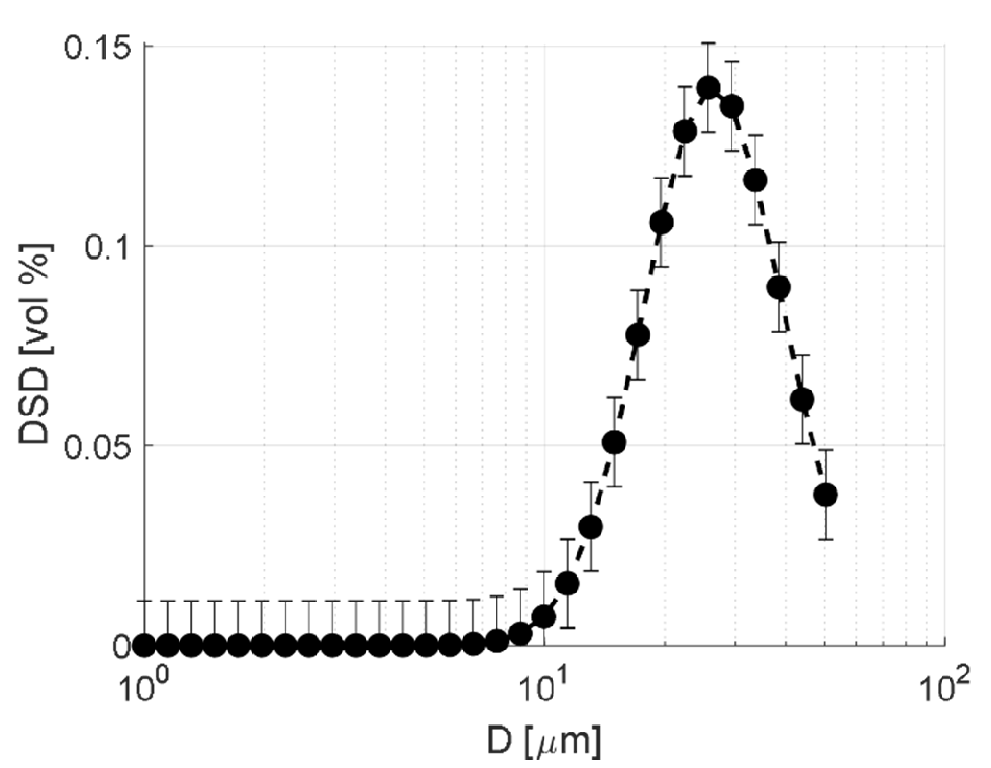
with parameters p = ln(50 × 10−6) and q = 0.4. This corresponds to a volume-averaged diameter of D43 = 37 µm. Figure 1 illustrates the initial DSD used in the study. After setting a fragmentation rate, g, and daughter drop distribution, f, a PBE discretized with the fixed pivot technique [53], with 30 size classes (the smallest class diameter pivot was set to 1 µm and vi/vi−1 = 1.5) was used to calculate the DSD after between 1 and 20 passages. Each passage was assumed to be the equivalent of 10 µs, estimated as the time the drops would spend in the intense turbulent field where breakup takes place. Note that the choice of the passage time will not influence the reliability or validity of the estimate, it only set the basis for the numerical value of g.
3.2.2. The Five Tests
Each method was subjected to five tests. The first test (I) investigates if the methods result in reliable estimates when fed with noisy data (provided that the assumptions made in the method were true). One set of synthetic data was generated for each method; making sure to use the same g and f that was assumed by the researchers originally suggesting the methods (see Table 2). A 4% relative uncertainty was added to the DSD (constant between size classes).
The second investigation (II) was carried out to study how reliable the methods are. To the synthetic dataset generated for each method, was added noise representing between 1 and 64% relative uncertainty to the DSD. The uncertainty for the estimated g was calculated using the Monte Carlo approach (see Section 3.1), for each of the four methods.
Investigation I and II assume that the fragment size distribution is known a priori. However, this is rarely the case; the shape of f as controversial as that of g [18,32,33,34]. The third and fourth investigations (III and IV), thus, tests how the estimated g is influenced when the different methods are fed with faulty assumptions about f. Since the daughter size distribution can be thought of as a combination of two factors—the general shape and the average number of fragments formed per breakup [68]—these investigations were divided in two. In investigation III, it was assumed that the shape of the daughter size distribution was known, but that the number of fragments formed per breakup was unknown. In investigation IV, the number of fragments was assumed to be known (m = 4), whereas f was assumed to be unknown. The synthetic data was generated by assuming that each fragmentation event gives rise to 4 equally formed fragments:
where δ denotes the Dirac distribution.
Each fragmentation rate extraction method was, however, evaluated using three different distinctively different fragment size distributions: a uniform probability function:
a beta (‘U-shaped’) fragment size distribution [69]:
and the true set f (Equation (21)).
Tests I–IV are based on the assumptions made about the shape of g by each method being true. However, the shape of g is highly contested [18,32,33,34], and a suitable method should be able to handle cases when g takes a more realistic (general) form. To test the sensitivity of the methods to the assumed shape of g, synthetic data was generated using a parameter-free fragmentation rate model [19], that has been widely used and expanded upon in subsequent studies [16,36,70]. Conditions similar to the breakup of an oil drop in water by an industrially relevant emulsification device were chosen (ρC = 998 kg/m3, μC = 10−3 Pa s, γ = 20 mN/m and ε = 105 m2 s−3).
The number of Monte Carlo attempts was set to NMC = 1000 for all tests. Doubling this number never influences average or standard deviations more than 5%. Results are therefore expected to be insensitive to the choice of NMC.
Table 2 summarizes the settings in terms of which g and f are used for each of the four methods, and for each of the five investigations. The numerical scales were chosen so that the fragmentation rates at an intermediary drop diameter (D = 30 µm) would be comparable, to make sure that the extent of fragmentation would be similar between cases.
The initial DSD was generated with Equation (18). Fragment size distribution was assumed to follow Equation (19) (m = 4) when generating synthetic validation data.
4. Results and Discussion
4.1. Validity under Uncertain Inputs (Test I)
Experimental DSDs are associated with some degree of measurement uncertainty. Experimentally, this is handled by repeating experiments several times, evaluating the results from each experiment separately, and drawing conclusions about the obtained average. Thus, a necessary condition for a suitable method for estimating the fragmentation rate is that it reproduces the set fragmentation rate as the average when applied on a large number of datasets, each of which is associated with measurement uncertainty, assuming that none of the assumptions made by the method are violated.
Figure 2 displays how each of the four methods performs in estimating the fragmentation rate when fed with DSDs where the relative uncertainty was set to 4%, which corresponds to a reasonable degree of experimental uncertainty in an emulsification experiment. (To illustrate what this degree of relative input uncertainty corresponds to in an experimental setting error bars representing 4% have been inserted in Figure 1).
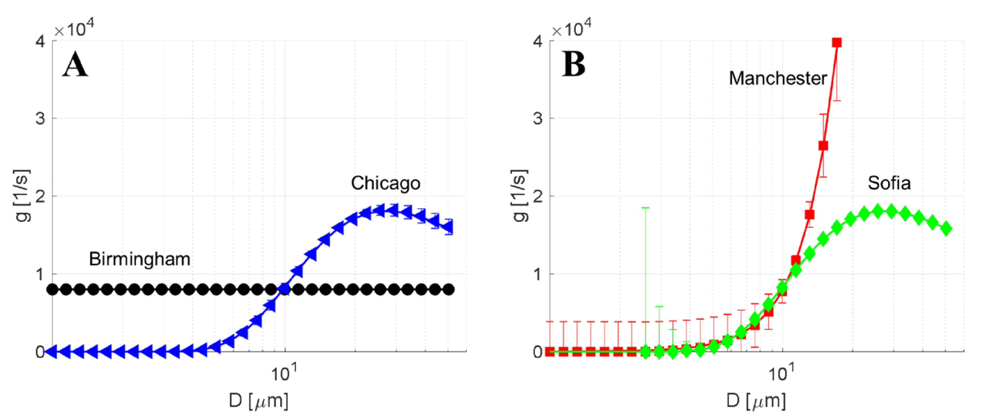
For each method, the solid line in Figure 2 shows the set fragmentation rate. (Note that these differ between the methods since the methods differ in what assumptions they make on how g depends on drop diameter, see Table 2). The symbols show the average estimated fragmentation rate of the 1000 evaluations (=NMC), and the error bars show the standard deviation across these individual ‘experiments’ (expanded uncertainty). As seen in the figure, the markers overlap the line, showing that all methods are able to reproduce the set fragmentation rate on average, as expected—at least when fed with experimental data with a relatively low degree of uncertainty and when all the assumptions used in the respective methods are met.
4.2. Reliability (Test II)
As seen already in Figure 2, the error bars vary between the methods, indicating that although each method, on average, predicts the correct fragmentation rate, the uncertainty obtained when applying the method on a specific set of experimental data will differ. Moreover, the error bars differ in length across the drop size axis.
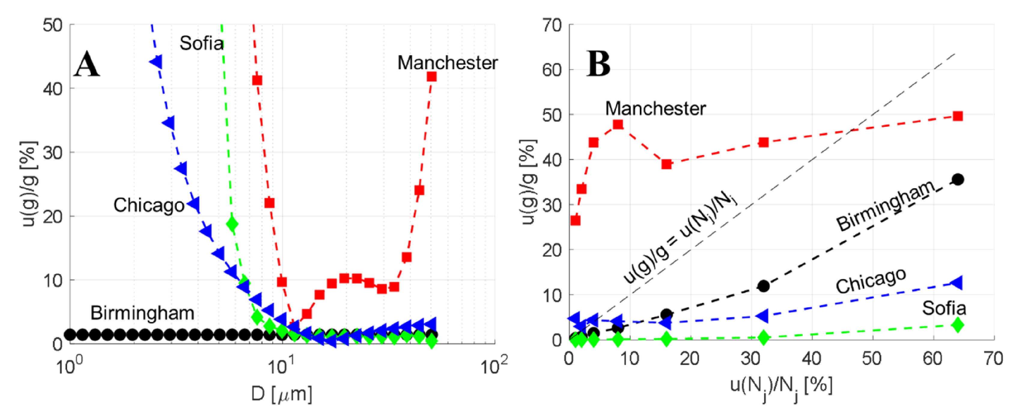
Figure 3A shows the relative uncertainty obtained in estimating the fragmentation rate with each of the four methods, as a function of drop diameter. First, note that the uncertainty in the estimated fragmentation rate typically varies greatly between different size classes. The Chicago and Sofia methods give a relatively high uncertainty for small drop sizes but a low uncertainty for larger drop sizes. The Manchester method gives a relatively high uncertainty throughout but performs best in a narrow interval of intermediary large drop sizes. The Birmingham method assumes that g has no size dependence and, consequently, estimates the fragmentation rate in each size class with the same uncertainty. Moreover, note that none of the methods based on a size-dependent fragmentation rate are able to reliably estimate the fragmentation rate of the smallest drops (D < 6 µm). However, this is not a limitation in the methods as much as a consequence of the imposed fragmentation rates; physically reasonable fragmentation rates tend to be near zero for ‘small’ drop diameters. When fragmentation rates are close to zero (in absolute terms), the obtained DSD are insensitive to small relative changes, thus making the resulting uncertainty in the g relatively large.
Figure 3B displays the resulting relative uncertainty in the fragmentation rate of a 30 µm drop as a function of the uncertainty in the DSD, comparing the four different methods. As expected, the output uncertainty (vertical axis), increases with the input uncertainty (horizontal axis). An x = y line (dashed) has been inserted to show under what conditions output uncertainty is higher or lower than input uncertainty. As seen in the figure, the Manchester method results in substantially less reliable results than the others. This is also in agreement with what was seen already in Figure 3A—the Manchester method only produces reliable results in a narrow span of drop sizes (D~10 µm). Returning to Figure 3B, also note that the Birmingham, Sofia, and Chicago methods result in relative uncertainties that are lower than the relative uncertainty in the input size classes (i.e., lines are below the dashed x = y line). A sub-proportionality scaling could seem contra-intuitive at first but can be understood from the fact that these three methods estimate g from a regression on DSDs measured after different numbers of passages (20 in this comparison), and the uncertainties in different size classes are (by assumption) uncorrelated to each other. As seen in Figure 3B, this gives rise to a canceling-out effect, reducing uncertainty in the Birmingham, Chicago, and Sofia estimates. That the Manchester method does not have this property indicates that it is substantially poorer in terms of reliability.
The relatively high reliability for the Sofia methods is particularly interesting given its large number of fitted parameters (I = 30 parameters), compared to the Chicago method (two parameters) and the Manchester method (three parameters). This relatively high reliability of the Sofia methods comes from the success of its back-calculation approach. Since each size-class is handled separately, the uncertainty in estimating the size class i, gi, is only influenced by uncertainties in larger size classes, resulting in that each gi has a relatively low uncertainty when i is large (and if i is small, no method would be able to determine it reliably anyway, due to the limitations with size classes where little fragmentation occurs, as discussed above).
In summary, test II shows that all methods except the Manchester have high reliability and that the reliability is highest for the Sofia method.
4.3. Sensitivity to the Number of Fragments Formed Per Breakup (Test III)
Thus far, all comparisons have been carried out by postulating that the daughter drop size distribution is known when analyzing an experiment; e.g., when investigating the reliability in Figure 2 and Figure 3, it was assumed that all fragmentation events resulted in the formation of m = 4 equally sized fragments. However, when using these methods on data from emulsification experiments, f is as unknown as g. In a realistic application of the fragmentation rate estimation methods, the experimentalist would use prior knowledge to guess f, apply the method and evaluate. In order to test how valid estimates of the fragmentation rate this approach would result in, each of the synthetic datasets (obtained assuming m = 4) were evaluated under the assumption of m = 2, m = 4, and m = 8.
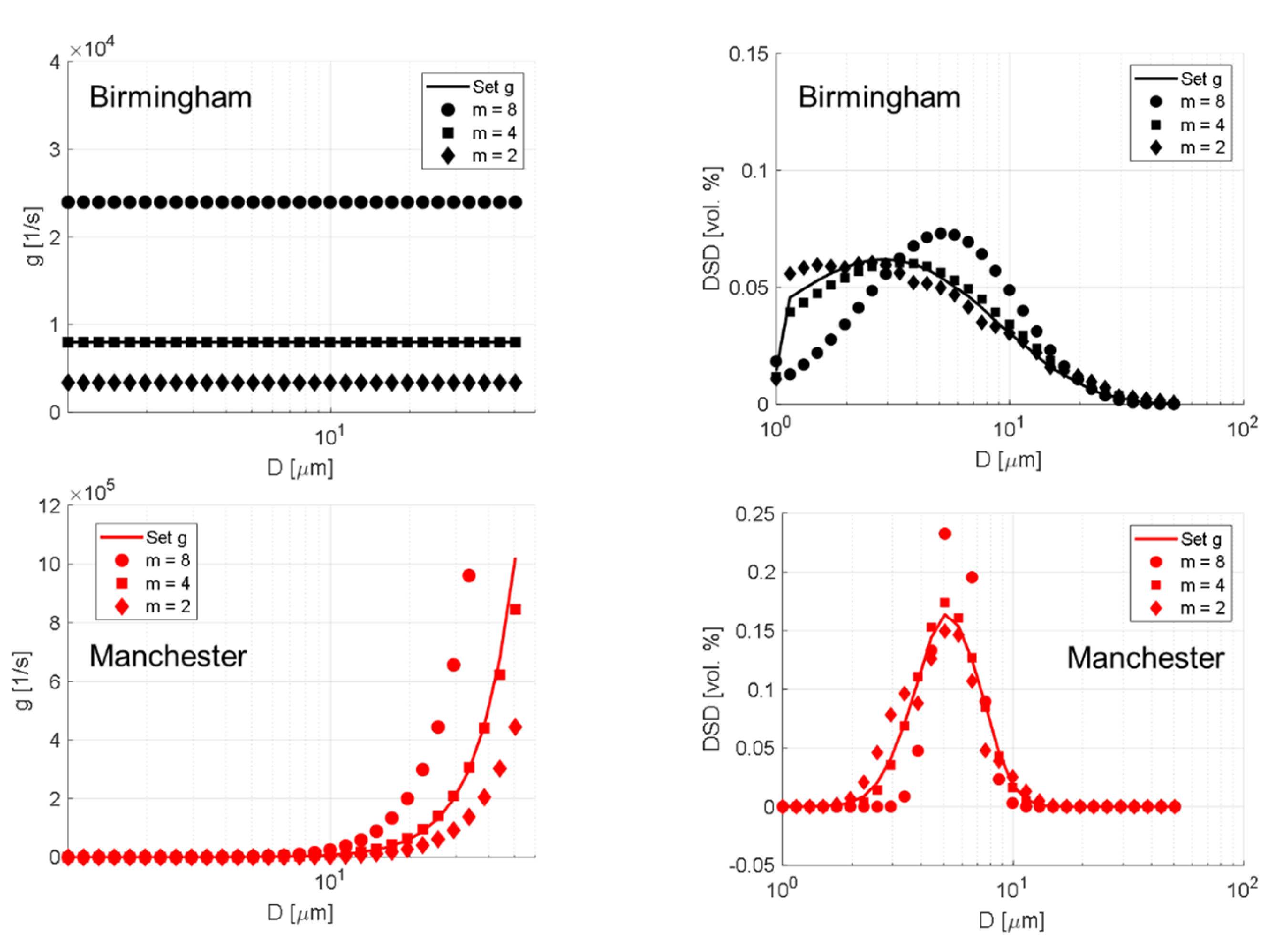
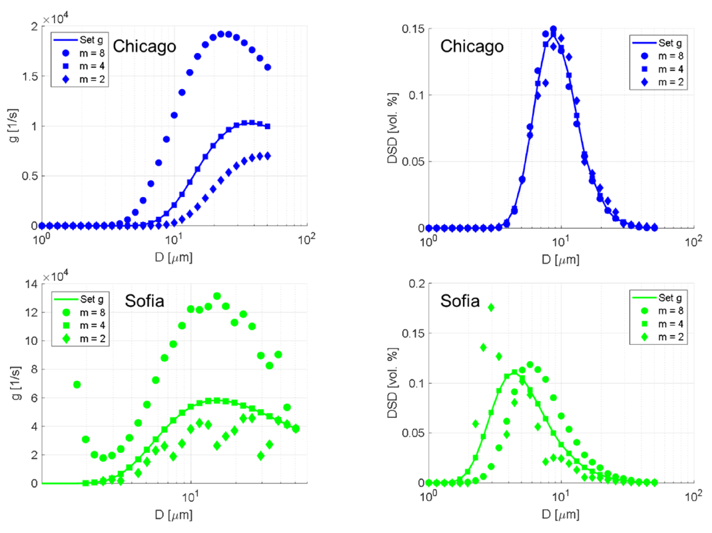
The left columns of Figure 4 and Figure 5 show the estimated fragmentation rates for the four methods (fragmentation rate in each size class). Each pane shows the estimates based on the three different assumptions about what the number of fragments formed per breakup actually is (circles: two fragments, squares: four fragments, and diamonds: eight fragments). In each pane, the true fragmentation rate (corresponding to the creation of four fragments) is illustrated with a solid line. Figure 4 displays the results for the Birmingham method (upper left) and the Manchester method (lower left). Figure 5 shows the results for the Chicago method (upper left) and the Sofia method (lower left). As seen in the figures, the g estimates are heavily dependent on the assumed value of m—underestimating m leads to a substantial underestimation of g.
However, this is not necessarily a problem. After g has been estimated, it can be used (together with the assumed m and f) to calculate a predicted DSD, by solving the forward discretized PBE (Equation (13)). This allows for a direct comparison with the actual resulting DSD which is typically available in an experimental setting. The right column in Figure 4 and Figure 5 shows the synthetic experimental DSD data after the last passage. Each pane shows the predicted resulting DSD with all three assumptions on the number of generated fragments. The resulting DSD generated with the true fragmentation rate is shown as a solid line (this corresponds to the measured DSD when using the method in an experimental setting). As seen, the appropriate value of m can be identified from the predicted DSD that fits the experimental DSD best (i.e., m = 4 gives the highest fit for all four methods). Relying on graphical similarity is, however, not ideal when using a fragmentation rate measurement method in an automatic setting. Thus, it would be beneficial to have access to a statistical measure for comparison. Table 3 shows the sum of squares residual (SSR) and the coefficient of determination (R2) for the different comparisons. In particular, the SSR shows a clear minimum when the correct guess is provided. Note that this methodology works for all four methods.
In summary, test III shows that not knowing the number of fragments formed (while still knowing the shape of f), does not represent a major challenge for any of the methods, since each method can be evaluated by assuming different values of m, and then inspecting which of these give the closest fit to the experimentally measure DSD.
4.4. Sensitivity to the Shape of f (Test IV)
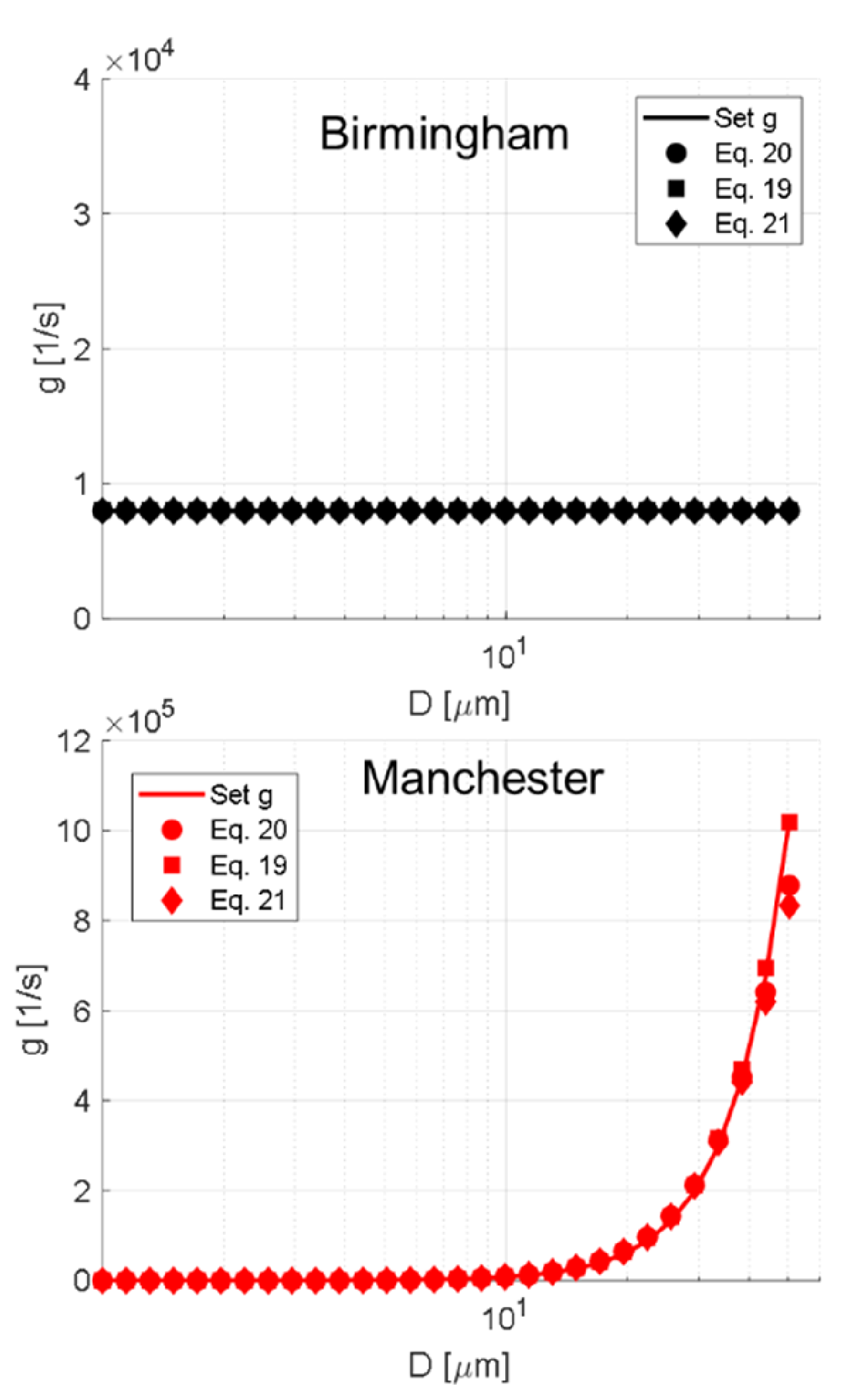
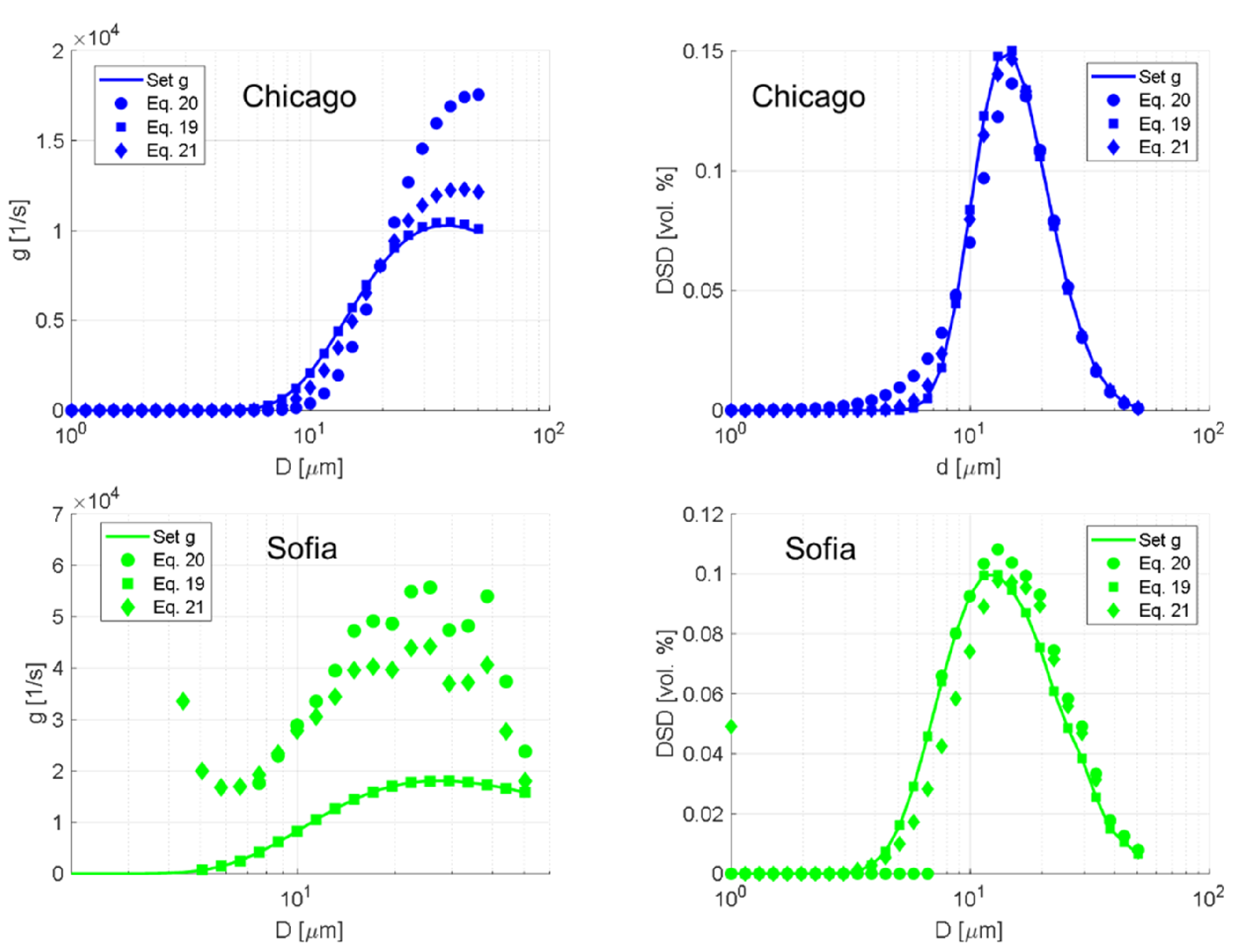
Figure 6 and Figure 7 show the result of a similar investigation to that described in Section 4.3 but relaxing the assumption that the shape of f is known a priori. The synthetic experimental DSD was generated assuming breakup into equally sized fragments (Equation (19)), but the obtained synthetic experiment DSDs were evaluated with three different assumptions on the shape of f; uniform probability (Equation (20)), beta-shaped (Equation (21)) and equally sized fragments (Equation (19)). Each pane in the left column shows three fragmentation rate estimations, one based on each assumption about the shape of f. Figure 6 displays the estimated fragmentation rate using the Birmingham and Manchester methods. Figure 7 shows the estimated fragmentation rate using the Chicago and Sofia methods. The true fragmentation rate has been illustrated using a solid line in each pane.
First note that the fragmentation rate estimations with the Manchester and Birmingham methods are insensitive to the assumed f as long as m is known (i.e., symbols in Figure 6 overlap)—since they are based on the zeroth moment of the DSD which is independent on the fragment size probability distribution (see Equations (5) and (12)). This illustrates the advantage of using a low complexity method.
The Sofia and Chicago methods, on the other hand (Figure 7), both give rise to systematic errors when f is not correctly specified (i.e., only estimates based on the correct assumption on f coincide with the solid line of the true fragmentation rate). However, if we have access to a closed set of potential f shapes [68], we could use the same method of identifying it as was used for determining an unknown m; measuring g based on each assumed f, calculating the corresponding DSD prediction, and comparing to the experimental DSD, just as in Section 4.3. The right column of Figure 7 displays the resulting DSD based on the three different assumptions on the shape of f, compared to the true DSD (corresponding to the measured DSD under experimental conditions). As in Section 4.3, it is possible to identify the correct assumption from looking at the similarity between true DSD and estimated DSD. Table 4 summarizes the SSR and R2 values for these investigations. Just as in Section 4.3, minimal SSR can be used as a method of identifying the correct shape of f.
In summary, test IV shows that not knowing the shape of f is not necessarily a major challenge for any of the methods. The Birmingham and Manchester methods are insensitive to the form of f, whereas a test-and-compare procedure can be used to identify an appropriate f for the Chicago and Sofia methods.
4.5. Sensitivity to Assumed Shape of g (Test V)
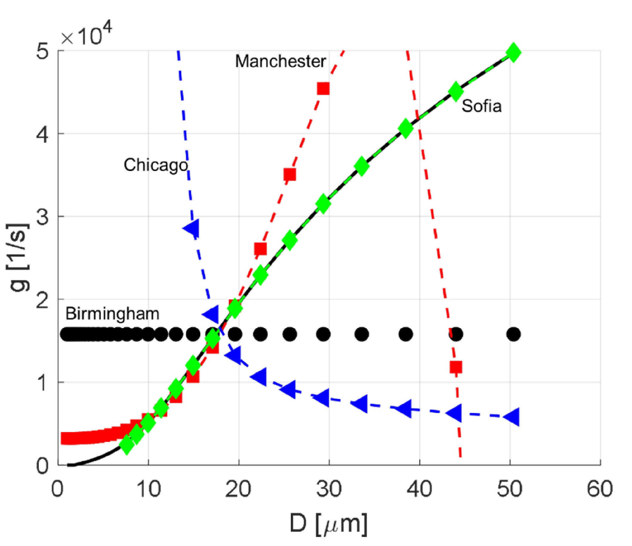
All comparisons thus far have been carried out under the assumption that that the fragmentation rate, g, has a shape consistent with that assumed by the authors deriving the different methods; e.g., the Birmingham method has been tested with a drop size-independent fragmentation rate and the Manchester method has been tested with a polynomial fragmentation rate (see Table 2 and Figure 2). However, as noted in the introduction, the form of the drop size dependence in g is contested. Moreover, this lack of knowledge in how the fragmentation rate depends on input and operating parameters is the main motivation for establishing rate estimation methods. Thus, it is interesting to test how well the four methods would fare when subjected to emulsification data coming from an emulsification process characterized by an independently set and more realistic fragmentation rate. Test V, therefore, applies the methods to synthetic data generated with the parameter-free fragmentation kernel [19].
Figure 8 shows the specified fragmentation rate (solid black line) and the estimations of g obtained when using each of the four methods. As expected, the Birmingham method (which is limited to the case of a size-independent kernel) fails to capture the size dependence. However, it does provide an estimate close to the average across size classes.
The estimation obtained with the Manchester method correctly estimates the fragmentation rate in a narrow region of approximately 10 < D < 20 µm but fails to capture the dependence of larger (and smaller) drops. Moreover, the Manchester method predicts an oscillating fragmentation rate with a sharp decrease for D > 35 µm. Both of these phenomena are consequences of the attempt of fitting a second-degree polynomial to a fragmentation rate that does not have a polynomial shape. From a Taylor-series expansion line of argument, we expect the estimate to fit a narrow interval, but diverge further from it. Attempts with changing the number of polynomial terms in the fitting (1–5) did not improve the fit between set and estimated fragmentation rate.
The Chicago method provides an estimate that shows an inverse behavior to the set fragmentation rate, indicating that it fails to find parameters p1 and p2 that make the Coulaloglou and Tavlarides kernel [46] fit the Lou and Svendsen kernel [19]. This illustrates the general challenge of using parametric determination methods for measuring fragmentation rates. As seen above, the method does works well as long as the shape of the fragmentation rate does follow the prescribed form (i.e., it is valid, reliable, and insensitive to m and f). However, as seen in Figure 8, the Chicago method is unable to provide any realistic estimate when facing an emulsification process characterized by a different fragmentation rate shape.
The Sofia method, on the other hand, provides a near-perfect fit to the set data, especially in the larger size classes, and the estimates still have high reliability (u(g)/g < 5% for D > 7 µm, with u(N)/N = 4%, Figure 8). This is also expected since the Sofia method makes no additional assumption on the shape of the fragmentation rate kernel.
4.6. Computational Cost
The four methods differ in computational cost. This can become an important factor when comparing large numbers of experiments. Table 5 shows the computational cost, in physical time units (per 1000 evaluations), for a typical laptop such as would be used to evaluate experimental results in the lab, together with the relative computational cost as compared to the fastest method. The estimations correspond to test I, i.e., each of the methods was fed with fragmentation rates and fragment size probability functions in accordance with the assumptions underlying it.
As seen in Table 5, both the Birmingham and Manchester methods are exceedingly fast, as expected when based solely on linear regressions. The Sofia method results in a higher computational cost since it requires—in addition to one linear regression (for the largest size class)—I − 1 non-linear regression. Note that the evaluation time is still short enough not to constitute a bottleneck (a single evaluation takes less than a second). A reason why computational time is still relatively low is that each non-linear regression will automatically be fed with a suitable initial condition from the larger size class.
The Chicago method results in, by far, the highest computational cost. The cost is substantial and will constitute a challenge when used under experimental conditions. The high computational cost can be attributed to the relatively slow convergence of the non-linear regression. Note that this is for the case where the regressions do eventually converge (the computational cost for test V, where the Chicago method fails to converge to a reasonable estimate, is substantially higher). It should be pointed out that the computational cost of the methods can likely be reduced by improving the numerical implementations, but such a numerical code optimization is outside the scope of the current investigation.
4.7. Comparison and Suggestions
Summarizing the investigations thus far: all four methods provide valid estimates when fed with experimental data carrying some uncertainty (test I, Figure 2). The methods differ in how sensitive they are to uncertainty in the experimental input; the Manchester method has the lowest reliability and the Sofia method has the highest (test II, Figure 3).
Moreover, for all of the methods, it was possible to obtain a valid estimate of g even when the number of fragments formed per breakup and the shape of f were unknown—at least if we know a set of such kernels including the actual one (tests III and IV, Figure 4, Figure 5, Figure 6 and Figure 7). Furthermore, the Manchester method was unable to provide a valid estimate of g when fed with a realistic fragmentation kernel (test V, Figure 8). Thus, the Manchester method is not a suitable candidate for further investigations.
Nor is the Chicago method considered a good candidate. The computational time is high (although this could potentially be reduced by optimizing the algorithm). A more severe limitation is that it is highly dependent on that the emulsification process proceeds according to a prescribed fragmentation rate form. As seen in Figure 8, it severely misrepresents the true rate when attempting to fit parameters to the wrong kernel. Although this could potentially be handled by guessing and testing different g shapes (e.g., from the library provided in reviews), it further increases computational costs and complexity, especially since the number of theoretically suggested fragmentation rate expressions is staggering—Solsvik et al. [34], identified 18 different sub-model classes in their comprehensive review from 2013 (each with several different suggested models), and new models are suggested regularly [26,35].
The Sofia method has good potential. It does not only have a low computational cost and high reliability when fed with experimental data with relatively high uncertainty (test II) but is also completely parameter free when it comes to g (test V). Thus, the Sofia method appears to be the best candidate for establishing a standard method for applied emulsification investigation of fragmentation rates.
The Birmingham method has a clear disadvantage in its inability to give any information about the size dependence of fragmentation rates. However, considering its simplicity, low computational cost, and that it does not require any information about the shape of f, one might wonder if the Birmingham method could still be a relevant tool for investigating fragmentation rates qualitatively. In a typical study emanating from the applied branch of emulsification studies, the experimentalist would be interested in how fragmentation rate scales with operating conditions (e.g., homogenizing pressure in a high-pressure homogenizer, or rotor speed in a rotor-stator mixer), or with the properties of the interface (e.g., with the type of emulsifier or interface rheology). An inability to capture the size dependence of the fragmentation rate might then be less problematic, as long as the method still captures the correct scaling.
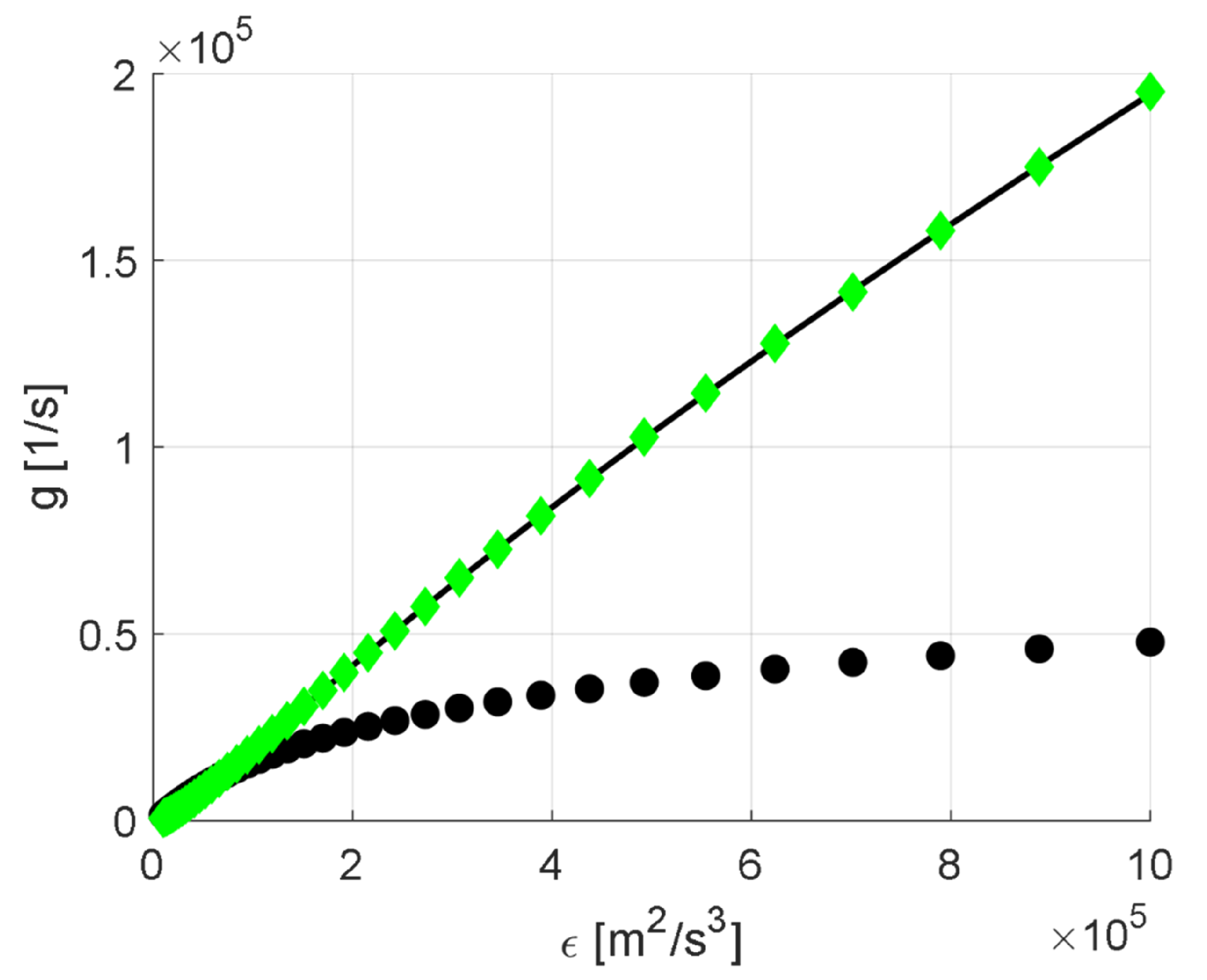
In order to test the Birmingham method’s ability to describe such a general scaling, the investigations underlying Figure 8 (test V) were repeated for a large number of dissipation rates of turbulent kinetic energy. This corresponds to running experiments with different rotor speeds or homogenizing pressures. Results can be seen in Figure 9. The solid line shows the true (set) fragmentation rate for a drop with 30 µm diameter, as a function of intensity. The green diamonds show the Sofia method estimates which, as expected, coincides perfectly with the set rate. The black circles show the estimates from the Birmingham method. As seen in Figure 9, the method somewhat overestimates how fast the fragmentation rate increases with intensity for low intensities and then underestimates it for higher intensities. However, the Birmingham method does estimate a monotonously increasing rate. Thus, if two emulsification conditions A and B (e.g., two different emulsifiers) were to give significantly different Birmingham-estimated fragmentation rates, gA > gB, this would be a valid argument for claiming that the conditions differ and to draw the conclusion that condition A gives rise to higher fragmentation rates than condition B. However, it would not provide quantitative information about how large the difference is (in neither relative nor in absolute terms).
5. Conclusions
The long-term objective of this research project is to find an easy-to-use, valid, and reliable method for estimating fragmentation rates; a method that could be used in applied emulsification investigations. Having access to such a method would be valuable, both for generating data to test theoretical models and for better understanding how operating conditions and emulsion properties influence the breakup behavior—fragmentation rate being a primary measure of breakup as compared to resulting drop size distribution, which is a secondary measure.
The specific objectives of this contribution were to systematically compare a subset of previously suggested methods in terms of (i) validity, (ii) reliability, and (iii) sensitivity to if emulsification conditions differ from those assumed to prevail when developing the methods.
The Sofia method (back-calculating based on a discretized PBE) [40,59] is identified as the most promising of all the methods. It provides a valid estimate even when fed with experimental data carrying some uncertainty, the relative uncertainty in the estimated fragmentation rate is low in comparison to the uncertainty in the measured drop size distribution, and the method does not require that the fragmentation rate has a certain specified drop size dependence.
The Chicago method (parameter fitting to a specified fragmentation rate expression) is less suitable since it severely misrepresents the fragmentation rate when the true size dependence deviates from the assumed one. Moreover, the computational cost is substantially higher than for the other method.
The two less complex methods (the Birmingham and Manchester methods), which both use trends in how the moments of the DSD change over time to estimate fragmentation rate, are unable to capture a realistic drop size dependence. However, the Birmingham method [50] (zeroth order Taylor polynomial) could be a valuable supplement to the more complex Sofia method, since it does provide a reliable (high reliability) estimate, allowing for qualitative comparison between experimental conditions.
Funding
This research was funded by The Swedish Research Council (VR), grant number 2018–03820, and Tetra Pak Processing Systems AB.
Institutional Review Board Statement
Not applicable.
Informed Consent Statement
Not applicable.
Data Availability Statement
Available at request from the corresponding author.
Conflicts of Interest
The author declares no conflict of interest.
References
- McClements, D.J. Food Emulsions: Principles, Practices, and Techniques; CRC Press: Boca Raton, FL, USA, 2016. [Google Scholar]
- Grace, H.P. Dispersion phenomena in high viscosity immiscible fluid systems and application of static mixers as dispersion device in such systems. Chem. Eng. Commun. 1982, 14, 225–277. [Google Scholar] [CrossRef]
- Kolmogorov, A.N. On the breakage of drops in a turbulent flow. Dokl. Akad. Nauk. SSSR 1949, 66, 825–828. [Google Scholar]
- Hinze, J.O. Fundamentals of the hydrodynamic mechanism of splitting in dispersion process. AIChE J. 1955, 1, 289–295. [Google Scholar] [CrossRef]
- Taylor, G.I. The formation of emulsions in definable fields of flow. Proc. Math. Phys. 1934, 146, 501–523. [Google Scholar] [CrossRef] [Green Version]
- Jafari, S.M.; Assadpoor, E.; He, Y.; Bhandari, B. Re-coalescence of emulsion droplets during high-energy emulsification. Food Hydrocoll. 2008, 22, 1191–1202. [Google Scholar] [CrossRef]
- Tcholakov, S.; Denkov, N.D.; Lips, A. Comparison of solid particles, globular proteins and surfactants as emulsifiers. Phys. Chem. Chem. Phys. 2008, 10, 1068–1627. [Google Scholar] [CrossRef]
- Håkansson, A. Emulsion formation by homogenization: Current understanding and future perspectives. Annu. Rev. Food Sci. Technol. 2019, 10, 239–258. [Google Scholar] [CrossRef]
- Gupta, A.; Eral, H.B.; Hatton, T.A.; Doyle, P.S. Controlling and predicting droplet size of nanoemulsions: Scaling relations with experimental validation. Soft Matter 2016, 12, 1452–1458. [Google Scholar] [CrossRef] [Green Version]
- Tadros, T.F. Emulsion Formation and Stability; Wiley-VCH: Weinheim, Germany, 2013. [Google Scholar]
- Tcholakova, S.; Denkov, N.D.; Danner, T. Role of surfactant type and concentration for the mean drop size during emulsification in turbulent flow. Langmuir 2004, 20, 7444–7458. [Google Scholar] [CrossRef]
- Atiemo-Obeng, V.A.; Calabrese, R. Rotor-stator mixing devices. In Handbook of Industrial Mixing; Paul, E.L., Atiemo-Obeng, V.A., Kresta, S.M., Eds.; Wiley: Hoboken, NJ, USA, 2004; pp. 479–505. [Google Scholar]
- Hall, S.; Pacek, A.W.; Kowalski, A.J.; Cooke, M.; Rothman, D. The effect of scale and interfacial tension on liquid–liquid dispersion in in-line Silverson rotor–stator mixers. Chem. Eng. Res. Des. 2013, 91, 2156–2168. [Google Scholar] [CrossRef] [Green Version]
- Mortensen, H.H.; Innings, F.; Håkansson, A. Local levels of dissipation rate of turbulent kinetic energy in a rotor–stator mixer with different stator slot widths—An experimental investigation. Chem. Eng. Res. Des. 2018, 130, 52–62. [Google Scholar] [CrossRef]
- Schultz, S.; Wagner, G.; Urban, K.; Ulrich, J. High-pressure homogenization as a process for emulsification. Chem. Eng. Technol. 2004, 27, 361–368. [Google Scholar] [CrossRef]
- Andersson, R.; Andersson, B. Modeling the breakup of fluid particles in turbulent flows. AIChE J. 2006, 52, 2031–2038. [Google Scholar] [CrossRef]
- Elghobashi, S. Direct numerical simulation of turbulent flows laden with droplets or bubbles. Annu. Rev. Fluid Mech. 2019, 51, 217–244. [Google Scholar] [CrossRef] [Green Version]
- Liao, Y.; Lucas, D. A literature review of theoretical models for drop and bubble breakup in turbulent dispersions. Chem. Eng. Sci. 2009, 64, 3389–3406. [Google Scholar] [CrossRef]
- Lou, H.; Svendsen, H.F. Theoretical model for drop and bubble breakup in turbulent dispersions. AIChE J. 1996, 42, 1225–1233. [Google Scholar] [CrossRef]
- Ramkrishna, D. Population Balances–Theory and Applications to Particulate Systems in Engineering; Academic Press: San Diego, CA, USA, 2000. [Google Scholar]
- Rivière, A.; Mostert, W.; Perrard, S.; Deike, L. Sub-Hinze scale bubble production in turbulent bubble break-up. J. Fluid Mech. 2021, 917, A40. [Google Scholar] [CrossRef]
- Rosti, M.E.; De Vita, F.; Brandt, L. Numerical simulations of emulsions in shear flows. Acta Mech. 2019, 230, 667–682. [Google Scholar] [CrossRef] [Green Version]
- Vela-Martín, A.; Avila, M. Deformation of drops by outer eddies in turbulence. J. Fluid Mech. 2021, 929, A38. [Google Scholar] [CrossRef]
- McClements, D.J. Critical Review of Techniques and Methodologies for Characterization of Emulsion Stability. Crit. Rev. Food Sci. Nutr. 2007, 47, 611–649. [Google Scholar] [CrossRef]
- Karimi, M.; Andersson, R. Dual mechanism model for fluid particle breakup in the entire turbulent spectrum. AIChE J. 2019, 65, e16600. [Google Scholar] [CrossRef] [Green Version]
- Andersson, R.; Andersson, B. On the breakup of fluid particles in turbulent flows. AIChE J. 2006, 52, 2020–2030. [Google Scholar] [CrossRef]
- Solsvik, J.; Jakobsen, H.A. A review of the statistical turbulence theory required extending the population balance closure models to the entire spectrum of turbulence. AIChE J. 2016, 62, 1795–1820. [Google Scholar] [CrossRef]
- Ashar, M.; Arlov, D.; Carlsson, F.; Innings, F.; Andersson, R. Single droplet breakup in a rotor-stator mixer. Chem. Eng. Sci. 2018, 181, 186–198. [Google Scholar] [CrossRef]
- Martínez-Bazán, C.; Montañés, J.L.; Lasheras, J.C. On the breakup of an air bubble injected into a fully developed turbulent flow. Part 1. Breakup frequency. J. Fluid Mech. 1999, 401, 157–182. [Google Scholar] [CrossRef] [Green Version]
- Solsvik, J.; Jakobsen, H.A. Single drop breakup experiments in stirred liquid-liquid tank. Chem. Eng. Sci. 2015, 131, 219–234. [Google Scholar] [CrossRef]
- Vejražka, J.; Zedníková, M.; Stranovský, P. Experiments on breakup of bubbles in a turbulent flow. AIChE J. 2018, 64, 740–757. [Google Scholar] [CrossRef]
- Lasheras, J.C.; Eastwood, C.; Martínez-Bazán, C.; Montañés, J.L. A review of statistical models for the break-up of an immiscible fluid immersed into a fully developed turbulent flow. Int. J. Multiph. Flow 2002, 28, 247–278. [Google Scholar] [CrossRef] [Green Version]
- Sajjadi, B.; Raman, A.A.A.; Shah, R.S.S.R.E.; Ibrahim, S. Review on applicable breakup/coalescence models in turbulent liquid-liquid flows. Rev. Chem. Eng. 2013, 29, 131–158. [Google Scholar] [CrossRef]
- Solsvik, J.; Tangen, S.; Jakobsen, H.A. On the constitutive equations for fluid particle breakage. Rev. Chem. Eng. 2013, 29, 241–356. [Google Scholar] [CrossRef]
- Bagkeris, I.; Michel, V.; Prosser, R.; Kowalski, A. Modeling drop breakage using the full energy spectrum and a specific realization of turbulence anisotropy. AIChE J. 2020, 67, e17201. [Google Scholar] [CrossRef]
- Solsvik, J.; Skjervold, V.T.; Han, L.; Lou, H.; Jakobsen, H.A. A theoretical study on drop breakup modeling in turbulent flows: The inertial subrange versus the entire spectrum of isotropic turbulence. Chem. Eng. Sci. 2016, 149, 249–265. [Google Scholar] [CrossRef]
- Henry, J.V.L.; Fryer, P.J.; Frith, W.J.; Norton, I.T. Emulsification mechanism and storage instabilities of hydrocarbon in-water sub-micron emulsions stabilized with Tweens (20 and 80), Brij 96v and sucrose monoesters. J. Colloid Interface Sci. 2009, 338, 201–206. [Google Scholar] [CrossRef] [PubMed]
- Lobo, L.; Svereika, A.; Nair, M. Coalescence during emulsification. 1. Method development. J. Colloid Interface Sci. 2002, 253, 409–418. [Google Scholar] [CrossRef]
- Taisne, L.; Walstra, P.; Cabane, B. Transfer of oil between emulsion droplets. J. Colloid Interface Sci. 1996, 184, 378–390. [Google Scholar] [CrossRef]
- Vankova, N.; Tcholakova, S.; Denkov, N.D.; Vulchev, V.D.; Danner, T. Emulsification in turbulent flow 2. Breakage rate constants. J. Colloid Interface Sci. 2007, 313, 612–629. [Google Scholar] [CrossRef]
- Hounslow, M.J.; Ni, X. Population balance modelling of droplet coalescence and break-up in an oscillatory baffled reactor. Chem. Eng. Sci. 2004, 59, 819–828. [Google Scholar] [CrossRef]
- O’Rourke, A.M.; MacLoughlin, P.F. A study of drop breakup in lean dispersions using the inverse-problem method. Chem. Eng. Sci. 2010, 65, 3681–3694. [Google Scholar] [CrossRef]
- Sathyagal, A.N.; Ramkrishna, D. Droplet breakage in stirred dispersions. Breakage functions from experimental drop-size distributions. Chem. Eng. Sci. 1996, 51, 1377–1391. [Google Scholar] [CrossRef]
- Håkansson, A. Experimental methods for measuring the breakup frequency in turbulent emulsification: A critical review. ChemEngineering 2020, 4, 52. [Google Scholar] [CrossRef]
- Raikar, N.B.; Bhatia, S.R.; Malone, M.F.; Henson, M.A. Self-similar inverse population balance modeling for turbulently prepared batch emulsions: Sensitivity to measurement errors. Chem. Eng. Sci. 2006, 61, 7421–7435. [Google Scholar] [CrossRef]
- Coulaloglou, C.A.; Tavlarides, L.L. Description of interaction processes in agitated liquid-liquid dispersions. Chem. Eng. Sci. 1977, 32, 1289–1297. [Google Scholar] [CrossRef]
- Maindarkar, S.N.; Hoogland, H.; Hansen, M.A. Predicting the combined effects of oil and surfactant concentrations on the drop size distributions of homogenized emulsions. Colloids Surf. A Physicochem. Eng. 2015, 467, 18–30. [Google Scholar] [CrossRef]
- Solsvik, J.; Becker, P.J.; Sheibat-Othman, N.; Jakobsen, H.A. Population balance model: Breakage kernel parameter estimation to emulsification data. Can. J. Chem Eng. 2014, 92, 1082–1099. [Google Scholar] [CrossRef]
- Kostoglou, M.; Karabelas, A.J. A contribution towards predicting the evolution of droplet size distribution in flowing dilute liquid/liquid dispersions. Chem. Eng. Sci. 2001, 56, 4283–4292. [Google Scholar] [CrossRef]
- Niknafs, N.; Spyropopoulos, F.; Norton, I.T. Development of a new reflectance technique to investigate the mechanism of emulsification. J. Food Eng. 2011, 104, 603–611. [Google Scholar] [CrossRef]
- Herø, E.H.; La Forgia, N.; Solsvik, J.; Jakobsen, H.A. Single drop breakage in turbulent flow: Statistical data analysis. Chem. Eng. Sci. X 2020, 8, 100082. [Google Scholar] [CrossRef]
- Masuk, A.U.M.; Salibindla, A.K.R.; Ni, R. Simultaneous measurements of deforming Hinze-scale bubbles with surrounding turbulence. J. Fluid Mech. 2021, 910, A21. [Google Scholar] [CrossRef]
- Kumar, S.; Ramkrishna, D. On the solution of population balance equations by discretization—I. A fixed pivot technique. Chem. Eng. Sci. 1996, 51, 1311–1332. [Google Scholar] [CrossRef]
- Azizi, F.; Al Taweel, A.M. Turbulently flowing liquid-liquid dispersions. Part I: Drop breakage and coalescence. Chem. Eng. J. 2011, 166, 715–725. [Google Scholar] [CrossRef]
- Konno, M.; Aoki, M.; Saito, S. Scale Effect on Breakup Process in Liquid-Liquid Agitated Tanks. J. Chem. Eng. Jpn. 1983, 16, 312–319. [Google Scholar] [CrossRef] [Green Version]
- Tsouris, C.; Tavlarides, L.L. Breakage and coalescence models for drops in turbulent dispersions. AIChE J. 1994, 40, 395–406. [Google Scholar] [CrossRef]
- Raikar, N.B.; Bhatia, S.R.; Malone, M.F.; McClements, D.J.; Henson, M.A. Predicting the effect of the homogenization pressure on emulsion drop-size distributions. Ind. Eng. Chem. Res. 2011, 50, 6089–6100. [Google Scholar] [CrossRef]
- Ribeiro, M.M.; Regueiras, P.F.; Guimaraes, M.M.L.; Madureira, C.M.N.; Cruz-Pinto, J.J.C. Optimization of breakage and coalescence model parameters in a steady-state batch agitated dispersion. Ind. Eng. Chem. Res. 2011, 50, 2182–2191. [Google Scholar] [CrossRef]
- Tcholakova, S.; Vanova, N.; Denkov, N.D.; Danner, T. Emulsification in turbulent flow: 3. Daughter drop-size distribution. J. Colloid Interface Sci. 2007, 310, 570–589. [Google Scholar] [CrossRef]
- Håkansson, A. An analytical solution to the fixed pivot fragmentation population balance equation. Chem. Eng. Sci. 2019, 208, 115150. [Google Scholar] [CrossRef]
- Håkansson, A. Estimating breakup frequencies in industrial emulsification devices: The challenge of inferring local frequencies from global methods. Processes 2021, 9, 645. [Google Scholar] [CrossRef]
- Joint Committee for Guides in Metrology. Evaluation of Measurement Data—Guide to the Expression of Uncertainty in Measurements. Available online: https://www.bipm.org/en/publications/guides/gum.html (accessed on 5 November 2021).
- Farrance, I.; Frenkel, R. Uncertainty of measurement: A review of the rules for calculating uncertainty components through functional relationships. Clin. Biochem. Rev. 2012, 33, 49–61. [Google Scholar]
- Farrance, I.; Frenkel, R. Uncertainty in measurement: A review of Monte Carlo simulation using Microsoft Excel for the calculation of uncertainties through functional relationships, including uncertainties in empirically derived constants. Clin. Biochem. Rev. 2014, 35, 37–60. [Google Scholar]
- Joint Committee for Guides in Metrology. Evaluation of Measurement Data—Supplement 1 to the “Guide to the Expression of Uncertainty in Measurements”—Propagation of Distributions Using Monte Carlo Methods. Available online: https://www.bipm.org/en/publications/guides/gum.html (accessed on 5 November 2021).
- Theodorsson, E. Uncertainty in measurement and total error: Tools for coping with diagnostic uncertainty. Clin. Lab. Med. 2017, 37, 15–34. [Google Scholar] [CrossRef] [PubMed]
- Walstra, P. Effect of homogenization on the fat globule size distribution in milk. Neth. Milk Dairy J. 1975, 29, 279–294. [Google Scholar]
- Diemer, R.B.; Olson, J.H. A moment methodology for coagulation and breakage problems: Part 3—Generalized daughter distribution functions. Chem. Eng. Sci. 1997, 57, 4187–4198. [Google Scholar] [CrossRef]
- Hsia, M.A.; Tavlarides, L.L. Simulation analysis of drop breakage, coalescence and micromixing in liquid–liquid stirred tanks. Chem. Eng. J. 1983, 26, 189–199. [Google Scholar] [CrossRef]
- Han, L.; Gong, S.; Li, Y.; Gao, N.; Fu, J.; Luo, H.; Liu, Z. Influence of energy spectrum distribution on drop breakage in turbulent flows. Chem. Eng. Sci. 2014, 117, 55–70. [Google Scholar] [CrossRef]
Figure 1.
The lognormal distribution used as the pre-emulsion DSD in the study. Error bars show plus/minus one expanded standard uncertainty, for the case of a 4% relative uncertainty (test I).
Figure 1.
The lognormal distribution used as the pre-emulsion DSD in the study. Error bars show plus/minus one expanded standard uncertainty, for the case of a 4% relative uncertainty (test I).

Figure 2.
Comparing estimated (symbols) and set (solid lines) fragmentation rates (g), as functions of drop size, D, for the four methods. All estimations are made on DSD data containing a relative uncertainty of 4%. Error bars denote resulting expanded uncertainty in g obtained, (A) The Chicago Method and The Birmingham Method, (B) The Manchester Method and The Sofia Method.

Figure 3.
(A) Relative uncertainty for each size class (comparing the four methods), when supplied with a low relative uncertainty in the drop size classes (4%). (B) Relative uncertainty in the size class corresponding to D = 30 µm, as a function of the relative uncertainty of the inputs.
Figure 3.
(A) Relative uncertainty for each size class (comparing the four methods), when supplied with a low relative uncertainty in the drop size classes (4%). (B) Relative uncertainty in the size class corresponding to D = 30 µm, as a function of the relative uncertainty of the inputs.

Figure 4.
Sensitivity of the different methods to the choice of m. Left column compares set fragmentation rates obtained by m = 4 (solid lines) to estimations using a range of assumed m-values (m = 2, 4, and 8). The right column compares the validation data DSD after 20 passages (solid lines), to the DSD predicted based on the different m-assumptions. Showing the Birmingham method (top row) and the Manchester method (lower row).

Figure 5.
Sensitivity of the different methods to the choice of m. Left column compares set fragmentation rates obtained by m = 4 (solid lines) to estimations using a range of assumed m values (m = 2, 4, and 8). The right column compares the validation data DSD after 20 passages (solid lines), to the DSD predicted based on different m assumptions. Showing the Sofia method (top row) and the Chicago method (lower row).

Figure 6.
Sensitivity of the different methods to the choice of f. Panes compares set fragmentation rates obtained by equal size fragments, Equation (19) (solid lines) to estimations using a range of assumed f shapes (circles: Equation (20), squares: Equation (19), and diamonds: Equation (21)). Showing the Birmingham method (top row) and the Manchester method (lower row).

Figure 7.
Sensitivity of the different methods to the choice of f. Left column compares set fragmentation rates obtained by equal size fragments, Equation (19) (solid lines) to estimations using a range of assumed f shapes (circles: Equation (20), squares: Equation (19), and diamonds: Equation (21)). The right column compares the validation data DSD after 20 passages (solid lines), to the DSD predicted based on the different f-assumptions. Showing the Sofia method (top row) and the Chicago method (lower row).

Figure 8.
Ability of the different methods to correctly estimate a realistic fragmentation rate (g), showing set g (solid line), compared to the estimates obtained with the four methods: Birmingham (circles), Manchester (squares), Sofia (diamonds), and Chicago (triangles).
Figure 8.
Ability of the different methods to correctly estimate a realistic fragmentation rate (g), showing set g (solid line), compared to the estimates obtained with the four methods: Birmingham (circles), Manchester (squares), Sofia (diamonds), and Chicago (triangles).

Figure 9.
Ability of the Sofia and Birmingham method to capture the dependence of g on turbulent intensity (as measured by the dissipation rate of turbulent kinetic energy, ε) with a realistic fragmentation rate. Solid line shows true (set) g. Black circles: Birmingham method. Green diamonds: Sofia method.


Table 1.
Assumptions imposed and experimental data required by the four investigated methods for estimating fragmentation rates from emulsification data.
Table 1.
Assumptions imposed and experimental data required by the four investigated methods for estimating fragmentation rates from emulsification data.
| Assumption on g(v) | Assumptions on m(v) | Assumptions on f(v,v′) | Experimental Data Required | |
|---|---|---|---|---|
| Birmingham [50] | g(v) ≡ G0. | m(v) ≡ m, assumed to be known | None | M0, initially and at a series of processing times or after different number of passages. |
| Manchester [41] | M0, M1, M2, …, initially and at a series of processing times or after different number of passages. | |||
| Chicago [46] | g(v) is known, except for a few (1–4) parameters | m(v) assumed to be known | f(v,v′) is known a priori, or externally fitted. | The DSD, initially and at a series of processing times or after different number of passages. |
| Sofia [40] | None |
Table 2.
Fragmentation rates used to generate the synthetic data in the different tests.
| Test | Birmingham | Manchester | Chicago | Sofia |
|---|---|---|---|---|
| I. Validity when fed with uncertainty data | g(v) = 8000 s−1 | g(v) = 25 + 4 106·(v/v0) +3.75·105(v/v0)2 s−1 | g(v) given by Equation (14) with p1 = 0.86 and p2 = 5.12 ρC = 998 kg/m3, ε = 105 m2/s3, φD = 1% | |
| II. Reliability | ||||
| III. Sensitivity to m | ||||
| IV. Sensitivity to f | ||||
| V. Sensitivity to g | g(v) from ref [19], with ρC = 998 kg/m3, μC = 10−3 Pa s, γ = 20 mN/m and ε = 105 m2 s−3 | |||
Table 3.
Sensitivity of the different methods to the choice of m. R2 and SSR between validation DSD and predicted DSD, making different assumptions of m, when using the methods to estimate the fragmentation rate. The validation data was created using m = 4 (‘CORRECT’).
Table 3.
Sensitivity of the different methods to the choice of m. R2 and SSR between validation DSD and predicted DSD, making different assumptions of m, when using the methods to estimate the fragmentation rate. The validation data was created using m = 4 (‘CORRECT’).
| m = 2 | M = 4 CORRECT | m = 8 | ||||
|---|---|---|---|---|---|---|
| R2 | SSR | R2 | SSR | R2 | SSR | |
| Birmingham | 95% | 0.054 | 100% | 0.0039 | 96% | 0.037 |
| Manchester | 75% | 0.25 | 99% | 0.0096 | 90% | 0.10 |
| Chicago | 94% | 0.28 | 100% | 1.8 × 10⁻⁵ | 97% | 1.7 |
| Sofia | 72% | 0.056 | 100% | 1.4 × 10⁻⁵ | <0 | 0.030 |
Table 4.
Sensitivity of the different methods to the choice of f. R2 and SSR between validation DSD and predicted DSD, making different assumptions of m, when using the methods to estimate the fragmentation rate. The validation data was created using equally sized fragment f (‘CORRECT’).
Table 4.
Sensitivity of the different methods to the choice of f. R2 and SSR between validation DSD and predicted DSD, making different assumptions of m, when using the methods to estimate the fragmentation rate. The validation data was created using equally sized fragment f (‘CORRECT’).
| Uniform Probability (Equation (20)) | Equally Sized Fragments (Equation (19)) CORRECT | Beta-Distribution (Equation (21)) | ||||
|---|---|---|---|---|---|---|
| R2 | SSR | R2 | SSR | R2 | SSR | |
| Chicago | 99% | 0.0059 | 100% | 4.3 × 10⁻⁵ | 100% | 8.2 × 10⁻⁴ |
| Sofia | <0% | 0.058 | 100% | 1.4 × 10⁻⁵ | 93% | 0.078 |
Table 5.
Computational cost across the four evaluating an experiment with the methods *.
| Method | Algorithm Dominating Cost | CPU Cost/1000 MC | Relative Computational Cost |
|---|---|---|---|
| Birmingham | Linear regression | 1 s | 1 |
| Manchester | Linear regression | 2 s | 2 |
| Sofia | I − 1 non-linear regressions | 2 min | 100 |
| Chicago | 1 non-linear regression | 3 h | 10,000 |
* On a PC laptop with 4 Intel Core i7 2.80 GHz processors.
Publisher’s Note: MDPI stays neutral with regard to jurisdictional claims in published maps and institutional affiliations. |
© 2021 by the author. Licensee MDPI, Basel, Switzerland. This article is an open access article distributed under the terms and conditions of the Creative Commons Attribution (CC BY) license (https://creativecommons.org/licenses/by/4.0/).
Share and Cite
MDPI and ACS Style
Håkansson, A. Towards a Standard Method for Estimating Fragmentation Rates in Emulsification Experiments. Processes 2021, 9, 2242. https://doi.org/10.3390/pr9122242
AMA Style
Håkansson A. Towards a Standard Method for Estimating Fragmentation Rates in Emulsification Experiments. Processes. 2021; 9(12):2242. https://doi.org/10.3390/pr9122242
Chicago/Turabian StyleHåkansson, Andreas. 2021. "Towards a Standard Method for Estimating Fragmentation Rates in Emulsification Experiments" Processes 9, no. 12: 2242. https://doi.org/10.3390/pr9122242
Note that from the first issue of 2016, this journal uses article numbers instead of page numbers. See further details here.