Scheduling Two Identical Parallel Machines Subjected to Release Times, Delivery Times and Unavailability Constraints


Industrial Engineering Department, College of Engineering, King Saud University, Riyadh 11421, Saudi Arabia
*
Author to whom correspondence should be addressed.
Processes 2020, 8(9), 1025; https://doi.org/10.3390/pr8091025
Submission received: 17 July 2020
/
Revised: 13 August 2020
/
Accepted: 17 August 2020
/
Published: 21 August 2020
(This article belongs to the Special Issue Optimization Algorithms Applied to Sustainable Production Processes)
Abstract
:This paper proposes a genetic algorithm (GA) for scheduling two identical parallel machines subjected to release times and delivery times, where the machines are periodically unavailable. To make the problem more practical, we assumed that the machines are undergoing periodic maintenance rather than making them always available. The objective is to minimize the makespan (). A lower bound (LB) of the makespan for the considered problem was proposed. The GA performance was evaluated in terms of the relative percentage deviation (RPD) (the relative distance to the LB) and central processing unit (CPU) time. Response surface methodology (RSM) was used to optimize the GA parameters, namely, population size, crossover probability, mutation probability, mutation ratio, and pressure selection, which simultaneously minimize the RPD and CPU time. The optimized settings of the GA parameters were used to further analyze the scheduling problem. Factorial design of the scheduling problem input variables, namely, processing times, release times, delivery times, availability and unavailability periods, and number of jobs, was used to evaluate their effects on the RPD and CPU time. The results showed that increasing the release time intervals, decreasing the availability periods, and increasing the number of jobs increase the RPD and CPU time and make the problem very difficult to reach the LB.
1. Introduction
Scheduling is a process of accomplishing determined tasks by effectively using restricted resources. Various scheduling problems have been investigated in various research fields, such as manufacturing operations [1], project management [2], construction [3], airline crew scheduling [4], outpatient appointments [5], maintenance [6], cloud manufacturing [7], and personnel scheduling [8]. Production scheduling is an important problem that has been widely investigated in the literature, such as the work presented by Pindo [9]. Production scheduling problem mostly refers to assigning a job to be processed in one or more machines in a specific sequence that leads to an optimal objective subjected to specific constraints. Abedinnia et al. [10] conducted a comprehensive literature review of the production scheduling problem.
Parallel machines scheduling problem refers to assigning a set of jobs for a specific number of identical machines by allocating each machine to a specific job(s) to optimize a specific objective(s) [11]. Each job must be processed in one machine. Alternately, each machine can only process one job at the same time. When the processing time of jobs is identical for all machines (machines have the same speed), the machines are called identical [12]. However, when the processing time depends on the machine and is different from one machine to another, either uniformly or arbitrary (unrelated), the machines are called nonidentical [13,14]. Many research studies in the literature have investigated the parallel machines scheduling problem with different objectives and constraints. The parallel machines scheduling problem has a different solution approach in the literature, depending on the desired objectives, which are related, but not limited, to minimizing the flow time [15], total/weighted tardiness [16,17], number of tardy jobs [18], and makespan [19]. In this context, the makespan is the maximum completion time when assigning each job to one machine [20]. The makespan objective, which is the objective of this research, has been studied in many production environments, rather than parallel machines, such as flow shop [21], job shop [22], flexible open shop [23], and single-machine scheduling problem [24]. Furthermore, various constraints have been addressed in the parallel machine scheduling problem, such as setup times [25], machine available times [26,27], ready times [28], release dates [29], and delivery times [30]. Release date, delivery date, and availability constraints have been investigated in the literature separately [27,31]. In this study, these constraints will be studied all together.
The release date refers to the arrival time of the task to the system [32]. In the literature, it has been studied as a constraint of different production environments. Liu et al. [33] presented a single-machine scheduling problem with release time. Other scheduling problems with release time are parallel machines [34], job shop [35], and open shop [36]. Moreover, the delivery time represents the period between the completion time of the job and its exit from the system [37]. Several studies have addressed the delivery time in different scheduling problems [38,39,40]. Another constraint that will be investigated in this research is the availability time. This constraint is due to preventive maintenance (PM) of the machines. PM should be well planned to minimize the makespan, considering that the jobs cannot be interrupted. In this regard, the machines are undergoing planned maintenance in a prespecific period, to maintain a well-defined operational performance. PM activities usually refer to lubrication, inspections, cleaning, alignment, replacement, adjustment, and repair [41]. The availability of machines was considered in machine scheduling in different situations. Since the machine in the real case will not be available all the time. Usually, machines are subjected to PM, sudden breakdowns, processing of special tasks or high-priority jobs, completing unfinished jobs from the previous period, or tool changes. These situations of machine unavailability were investigated in the literature [42,43,44,45,46,47,48,49,50].
The objective of this paper is to minimize the makespan of parallel machines with release dates, delivery dates, and machine availability constraints. To the best of our knowledge, no research study has investigated this problem. However, many reports in the literature have investigated the problem of minimizing the makespan of parallel machines with the release and delivery dates without considering machine availability [32,37,51].
2. Problem Description
The scheduling problem of two identical parallel machines subjected to release time, delivery time, and machine unavailability is formally defined as follows. A set of n jobs have to be processed by a set of identical parallel machines . Each job j has a release time from which it will be ready to be processed. Job j has a processing time and has to be processed on the available machines . A particular machine is available for a period of after which it will be unavailable for a time , a required time to conduct a PM action on the machine . Since the two machines are identical, the available and unavailable periods for the two machines will be considered to be the same. In other words, and . Each must spend a duration called delivery time after processing had been finished on the machine . The processing of all jobs on the identical parallel machines is conducted under the following assumptions:
- Each machine can process only one job at a time, and all jobs are non-preemptive.
- If machine is unavailable (down for a PM action), it will not be capable of processing jobs until is finished.
- PM activities can be done early (before the end of the period ), but for the possibility of failure occurring, they cannot be delayed.
- The machines are available for processing again after the unavailable period (PM activity).
- The release time , delivery time , and processing time for each job are known in advance.
- The availability and unavailability periods of a particular machine are deterministic and known in advance.
The objective is to minimize the makespan (). According to [37], the related problem without addressing machine’s availability and PM is an NP-hard problem. Therefore, the considered problem is NP-hard, and can be expressed using Graham’s notations as follows: . “” denotes the constraint of machine unavailability due to preventive maintenance (PM). The following notations will be used to define the considered problem:
- : number of jobs;
- : number of machines;
- : job’s index ();
- : machine’s index ();
- : processing time of job ;
- : release time of job ;
- : delivery time of job ;
- : starting time for processing job ;
- : machine available time;
- : machine unavailable time, the required time to perform a PM action;
- : completion time of job , ;
- : maximum completion time, max ().
The proposed objective function for the considered scheduling problem under investigation is stated as follows:
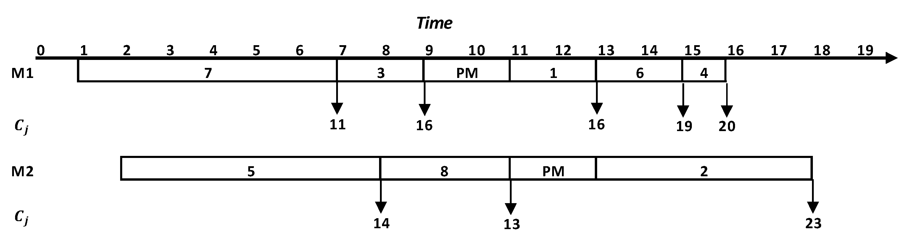
where can be calculated as , where . The following example illustrates the schedule construction of the considered problem, . Consider a set of eight jobs, with the processing times, release times, and delivery times as shown in Table 1. The jobs have to be scheduled on two identical machines: m1 and m2. The machine available periods and the unavailable periods, the required time for performing the PM actions, are presented in Table 2. For example, machine 1 is considered to be available for 9 units of time before a PM action, and then, it will be down (unavailable) for 2 units of time (under maintenance). Let the current job sequence be (7, 5, 3, 8, 1, 6, 2, 4). According to the given sequence, the jobs are assigned to the nearest available machine.
The constructed schedule of the given sequence is presented on a Gantt chart shown in Figure 1. From the sequence, job 7 is the first job to be scheduled. Since the two machines are available at time 0 and job 7 is ready at time 1 (), job 7 can be assigned to one of the two machines. Here, job 7 is assigned to , and it is processed for 6 units of time () starting at time 1 and finishing at 7. Job 7 has a delivery time of 4 units of time (), so its completion time is (1 + 6 + 4 = 11). The second job to be scheduled is job 5, which is available at time 2 (). Machine is available at time 2. Hence, job 5 is assigned to machine 2, and the starting processing time of job 5 is 2. Furthermore, it will be processed for 5 units (), finishing at time 8. Job 5 has a delivery time of 6 units of time (), so its completion time is . The rest of the unscheduled jobs will be scheduled on the same procedure until all jobs in are scheduled. Since machines are not always available as they need periodic PM, jobs cannot be processed when machines are under PM actions. From Table 2, machines 1 and 2 should have a PM every 9 operational times , and the required time to do the PM is 2 units . A PM for machine 1 will be performed for 2-unit times at time 9, despite machine 1 having worked for only 8 units of time. This is because job 1, the next scheduled job in , has a processing time of 2 units, which will exceed the availability period , and for the possibility of failure, the PM on machine 1 will be performed before starting processing job 1 at time 9. Machine 1 will be available again at time 11 and start processing job 1. Note that the machine will be in its best condition after the PM action. Machine 2 will be operated for 9 units until time 11, so it will be unavailable for 2 units. After finishing PM on machine 2, job 2 will be processed by machine 2. From Figure 1 the , for the given sequence, is 23.
It is worth mentioning that the number of jobs, processing times, release times, delivery times, and availability and unavailability periods affect the . For example, machine 1 will wait 1 unit of time for job 7 to be ready, and machine 2 will wait for 2 units for job 5 to be ready for processing. Besides, jobs 1 and 2 will wait for processing on machines 1 and 2, respectively, as they are not available.
For this problem, we propose the lower bound (LB) for the considered problem, , as follows:
Clearly, no job can be finished earlier than [37]. Furthermore, since the machine availability period must be greater than the maximum processing time such that
where is the machine availability period, an LB that is similar to that for the problem is as follows:
As machines are subjected to PM actions, the minimum PM times can be calculated based on [50,52]:
where is the machine availability period before a PM action is needed, and denotes the largest integer that is smaller than or equal to y.
The minimum time that a machine will not be available under PM activities can be calculated as follows:
where s is the PM time.
By adding the unavailable time due to the PM activities to the two LBs developed by [51] for the , we get the following LBs:
Ranking the jobs in an increasing manner as regards their release times and delivery times, such that and ( are the two smallest release times and are the two smallest delivery times), we get
3. Genetic Algorithm
Genetic algorithms (GAs) are adaptive metaheuristic search algorithms used for solving combinatorial optimization problems. GAs represent one branch in the field of evolutionary algorithms (EAs). GAs use natural evolution-inspired techniques in which they imitate the biological processes of reproduction and natural selection to solve for the “fittest” solutions [53]. GA was first proposed by Holland in 1975, in an attempt to solve some optimization problems by imitating the genetic process of living organisms and the law of the evolution of species [54]. In 1989, Golberg [55] applied GA to optimization and machine learning.
To solve the problem under study, we propose a GA to present high-quality solutions within allowable computing times. The reasons behind choosing the GA are its well-known reputation for high performance when solving combinatorial optimization problems, and more importantly, its effectiveness in solving related problems as reported in previous studies (see for example [14,17]). Several genetic operators are considered, and the selection of the best GA operator parameters has been optimized based on response surface methodology (RSM) experimental design, as detailed in Section 4.3. The proposed GA presents the following operators: generation of the initial population, fitness evaluation, parent selection, crossover, and mutation. In the next subsections, the GA main elements are discussed.
3.1. Chromosome Encoding
Genes are the main component to build GAs, since chromosomes are a sequence of genes. When building a GA for scheduling problems, each job in the schedule is represented as a gene in a chromosome. This operation, that is, representing individual genes, is known as encoding. Several encoding schemes are presented in related studies. The most used encoding scheme is the permutation encoding in which every chromosome is represented as a permutation list of jobs. A permutation list is a linear order list of all the jobs with no repeated values, where an extra gene is used to distinguish the machines on the chromosome. See Section 2 (Figure 1) for an illustration.
3.2. Initial Population
A population is a collection of chromosomes. In the GA, the two main aspects of a population are the size of the population and its initial generation process. Usually, the initial population is generated randomly. However, in some cases, for complicated problems, to increase the quality of the generated population, a small part of the initial population is generated using a problem-specific heuristic, and the rest is generated randomly to ensure population diversity. In the proposed GA, the population size is determined using a preliminary study as detailed in Section 4. However, the initial population is generated randomly to make sure the initial population is diverse.
3.3. Chromosome Evaluation
The evaluation process is used to compute the fitness value of each individual in the present population. In the evaluation process, the current population is evaluated by decoding each chromosome in that population and calculating its objective function value. As the generated chromosomes do not include the PM activities, the following procedure (Procedure 1) is required to decode each chromosome and calculate its objective value. In the proposed procedure, the evaluation starts by delivering all the inputs for parameters, including the randomly generated sequence . Starting with the first job of the sequence, there are two possibilities. The first is that the current machine age plus the processing time of that first job is less than or equal to the availability time of the machine before PM. Then, there is no PM, the machine’s age will be updated, the job will be scheduled on that available machine, the completion time of the scheduled job will be calculated, and finally, the machine availability will be updated. The second possibility is that the current machine age, plus the processing time of that first job, is larger than the availability time of the machine before PM. Then, a PM activity should be assigned to that machine first before scheduling the job. The starting and completion time of the PM activity is going to be determined. Then, the machine’s age and availability are going to be calculated. Finally, the job is going to be scheduled on the machine and the completion time of the scheduled job is going to be obtained. This process is going to be repeated for all the jobs in the input sequence . The final step of the procedure is to calculate as the maximum of all job’s completion times. All details can be found in the proposed procedure (Procedure 1).
3.4. Selection and Reproduction Process
The selection process ascertains the chromosomes that are chosen for mating and reproduction. The main purpose of the selection process is as follows: “the better an individual is, the higher its chance of being a parent.” In this study, Roulette wheel selection was used in which each individual is assigned a selection probability that is proportional to its relative fitness, . The selection of beta individuals is performed by beta-independent spins of the roulette wheel. Each spin will select a single individual, and the better individual will be selected. The roulette wheel selection operator is selected based on some preliminary experiments, it has been found that, for the problem under investigation, the roulette wheel selection operator performs better than the tournament selection operator and random selection. This was consistent with previous research (for example [14,17,53,56]), as they have suggested that roulette wheel selection operator is the best operator for scheduling problems.
3.5. Crossover
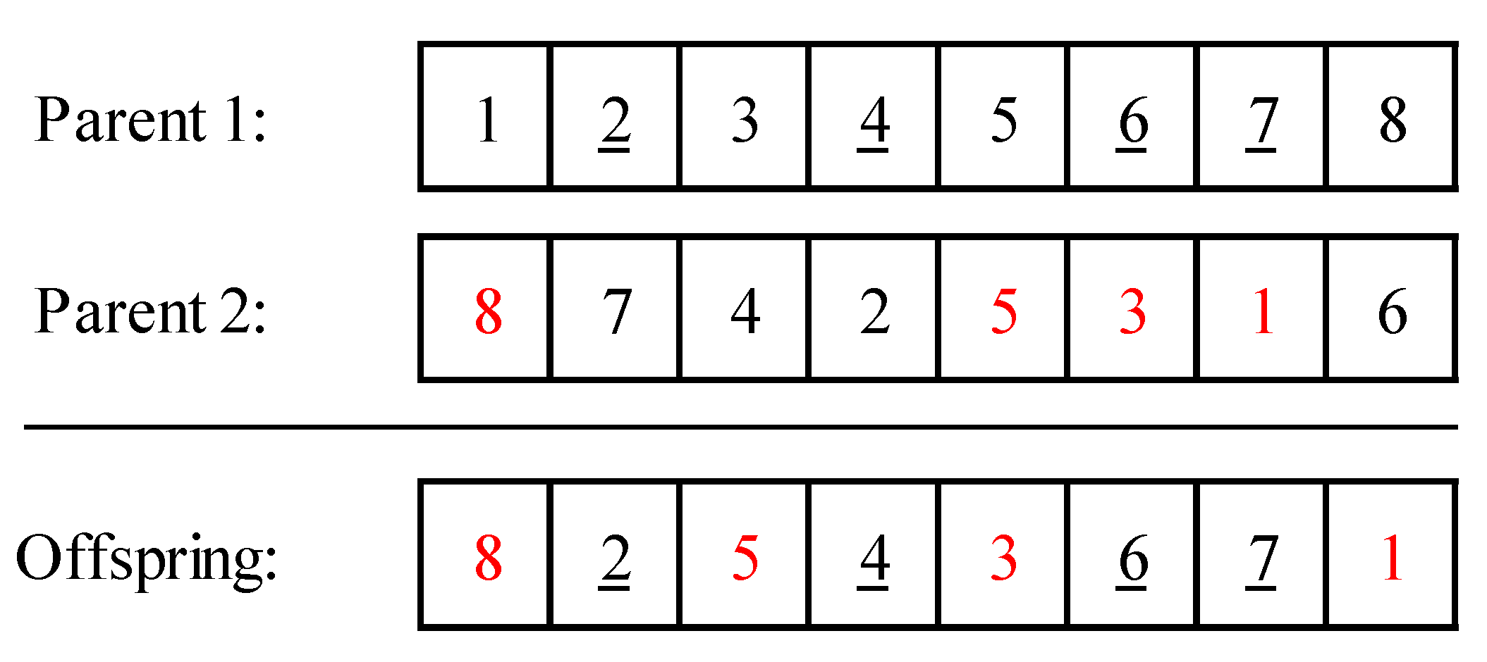
Reproduction in GA is conducted by applying crossovers and mutations. The crossover process consists of a combination of two parents to create a new child. The crossover operators were selected using a permutation list; that is, the proposed operator was applied to a permutation of coded operations. In this study, a position-based crossover (PBX) proposed by Syswerda [57] was used. In a PBX operator, a subset of positions from the first parent is randomly selected and copies the components at these positions to the offspring chromosome at the same position and then fills the other positions with the remaining components in the same order as in the second parent. An example of a PBX is given in Figure 2. The most important variable that needs to be tuned in the crossover process is the crossover rate , which represents the proportion of parents on which a crossover operator will occur.
| Procedure 1 Chromosome Evaluation | ||||
| 1 | Inputs: | |||
| is the number of jobs; is the number of machines, which is 2; are the processing times of each job; are the ready times of each job; are the delivery times of each job; is the machine available time; is the machine unavailable time; is the generated sequence (randomly generated as explained in Section 3.2); | ||||
| 2 | For , | |||
| ; and is the assigned machine; If is the 1st job in the assigned machine : | ||||
| If machine age + ; %% No PM action | ||||
| machine age = machine age + ; ; ; machine availability = ; | ||||
| Else%% PM action is required | ||||
| machine availability; ; machine availability = ; machine age = ; ; ; machine availability = ; | ||||
| End (if); | ||||
| Else | ||||
| If machine age + ; %% No PM action | ||||
| machine age = machine age + ; ; ; machine availability = ; | ||||
| Else%% PM action is required | ||||
| machine availability; ; machine availability = ; machine age = ; ; ; machine availability = ; | ||||
| End (if); | ||||
| End (if); | ||||
| End (for); | ||||
| 3 | Output: ; | |||
3.6. Mutation
Mutation occurs after crossover is completed. This operator applies the changes randomly to one or more “genes” to produce a new offspring. Hence, it creates new adaptive solutions good in avoiding local optima. The percentage of genes that will be mutated is denoted as Mu. Mutation probability (Pm) determines how many chromosomes (offspring) should be mutated in one generation. Pm is in the range of [0, 1]. In this paper, we used a combination of swap, reversion, and insertion mutation operators for producing the mutation offspring. Operators are selected randomly with equal probability, i.e., every time the mutation function was called by GA, one of the three operators will be randomly chosen with equal probability.
3.7. Replacement and Termination Condition
The replacement phase concerns the survivor selection of both the parent and the offspring populations. In this study, the population was updated based on elitism in which the best individuals are selecting from the parents and offspring. The GA preserves the solution with the best value of the objective function in the next generation when adopting elitism [57].
Computational time and convergence of the fitness value are considered simultaneously for terminating the GA iterations. In this paper, the search process will be terminated if the fitness reaches the LB, no improvement in the best fitness values of the current population values for a given number of successive iterations, or the number of iterations reaches the maximum allowable number. The algorithm is repeated until the termination condition is satisfied.
4. Experimental Design
In this section, we describe the design of the experiments performed to select the best GA parameters proposed in Section 3. In the next sections, we present the indicators used for the evaluations, describe the test instances, and discuss the selection of the GA parameters.
4.1. Indicator of the Evaluation
The statistics used in the analysis of the computational experiments to assess the performance of the proposed algorithm are based on the proposed LB presented in Equation (9). For each instance, the relative distance to the LB was calculated. Thus, for instance , the relative gap between the and is calculated using the relative percentage deviation (RPD), denoted as in Equation (9):
In addition to the RPD, the computation time taken to solve each instance was presented.
4.2. Description of Test Instances
To study the effect of the scheduling problem constraints, an experimental study based on the factorial design was conducted using a set of instances. The test instances were generated randomly based on the data set designed by previous studies. Two sets of processing times were similar to Liao et al. [42], and the sets were generated uniformly in the intervals of and . Two sets of release time times were uniformly distributed in the intervals of and , where a and b correspond to , n is the number of jobs, and m is the number of machines (m = 2). The first set was similar to that in [37], while the second one was generated so that the jobs arrive throughout the scheduling plan which makes the problem more practical. Two sets of delivery times were generated, with random values uniformly distributed in the intervals of , and considering the delivery time as a function of the processing time. Machine availability and unavailability periods were generated similarly to that in Liao et al. [42] considering the as a function of the processing times and number of jobs. Two sets of machine availability periods of were generated such that and . Two sets of machine unavailability periods were generated such that and .
For every combination of , , , and , different problem sizes of n jobs were generated where n ∈ (10, 20, 30, 40, 50, 100, 200, 300, 400, and 500). For each size, five instances were randomly generated. The summary of the instance characteristics of the problem is presented in Table 3.
4.3. Response Surface Methodology
The influence of the GA parameters, discussed in Section 3, on its performance was evaluated through an experimental design approach. RSM was used for the parametric study and optimization of the GA parameters for efficient solving of the scheduling problem under study. In this work, RSM’s face-centered central composite (FCC) design, a second-order experimental design with three levels, was employed to analyze the effects of the selected five GA parameters on output response ( and ). Based on the literature and a preliminary screening, five GA parameters and their respective levels were selected, as shown in Table 4. The design consists of a full factorial having 52 runs including 32 cube points and 20 center points (10 center points in a cube and 10 center points along the axis).
Analysis of variance (ANOVA) was performed to investigate the significance of the GA parameters and their interactions in relation to RPD and central processing unit (CPU) time. P-values less than 0.05 indicate model terms are significant. Model reduction was performed using the forward elimination process to improve the model by deleting insignificant terms without a statistically significant loss of fit. The data sets, that were used to experimentally optimize the GA’s parameters, were selected from the generated instances described in Section 4.2, taking into account the sample size, n ∈ (10, 500). The GA was run 10 times, and the average RPD and CPU time were reported for the selected instances.
Table 5 and Table 6 present the reduced ANOVA tables for the RPD and central processing unit (CPU) time, respectively. For the RPD, the population size, mutation ratio, and beta are statistically significant factors as their P-values less than 0.05 (Table 5). The interactions of the population size with mutation probability and beta are statistically significant. For the CPU time, the population size, mutation rate, and mutation probability are statistically significant (Table 6). The interactions of population size with mutation probability and mutation rate and the interactions of mutation probability with mutation rate are statistically significant. Note that the two-way interactions have a contribution of 36.04%, which indicates that a second-order model should be adapted for optimizing the GA parameters. It is worth noting that the normality assumption is satisfied and the adjusted R2 for the RPD and CPU time models are 90.14% and 82.45%, respectively.
The mathematical models in terms of actual factors have been obtained to make predictions and multiobjective optimization. The mathematical models of RPD and CPU time are given in Equations (10) and (11), respectively.
Desirability function, embedded in Minitab software, has been used for multiobjective optimization of the GA parameter settings. Desirability function is a mathematical method used for multiple response optimization, proposed by Derringer and Suich [58]. In the desirability function, each response is transformed into a desirability function that ranges from 0 to 1, where 0 is least desirable. Overall desirability of the multi-response system is measured by combining the individual desirabilities of the responses. The objective is to find parameter settings that maximize the overall desirability. In this study, the optimal solution is to minimize RPD and CPU time. Table 7 shows the optimal combination values of the GA parameters as a result of multiobjective optimization with overall desirability of 0.9867.
5. Results and Discussions
In this section, the effect of the scheduling problem variables on the RPD and CPU time is investigated. A full factorial experimental study is conducted using a set of instances generated randomly, described in Section 4.2, based on five factors, which are process times (p), release times (r), delivery times (q), availability period (t), unavailability period (s), and the number of jobs (). Two levels were considered for these variables except for the number of jobs in which there were 10 levels (Table 3), which resulted in the generation of 320 instances. Furthermore, every instance was generated five times. A total of 1600 instances was generated. The GA was run five times for every instance, and the average and CPU time was reported.
The proposed GA has been coded using MATLAB software (The MathWorks Inc., MA, USA), and the computational experiments for all instances have been conducted on the same computer with the following specifications: Intel® Core™ i5-3230M at 2.6 GHz for the CPU processor (Intel Corporation, CA, USA) and 4.0 GB for RAM.
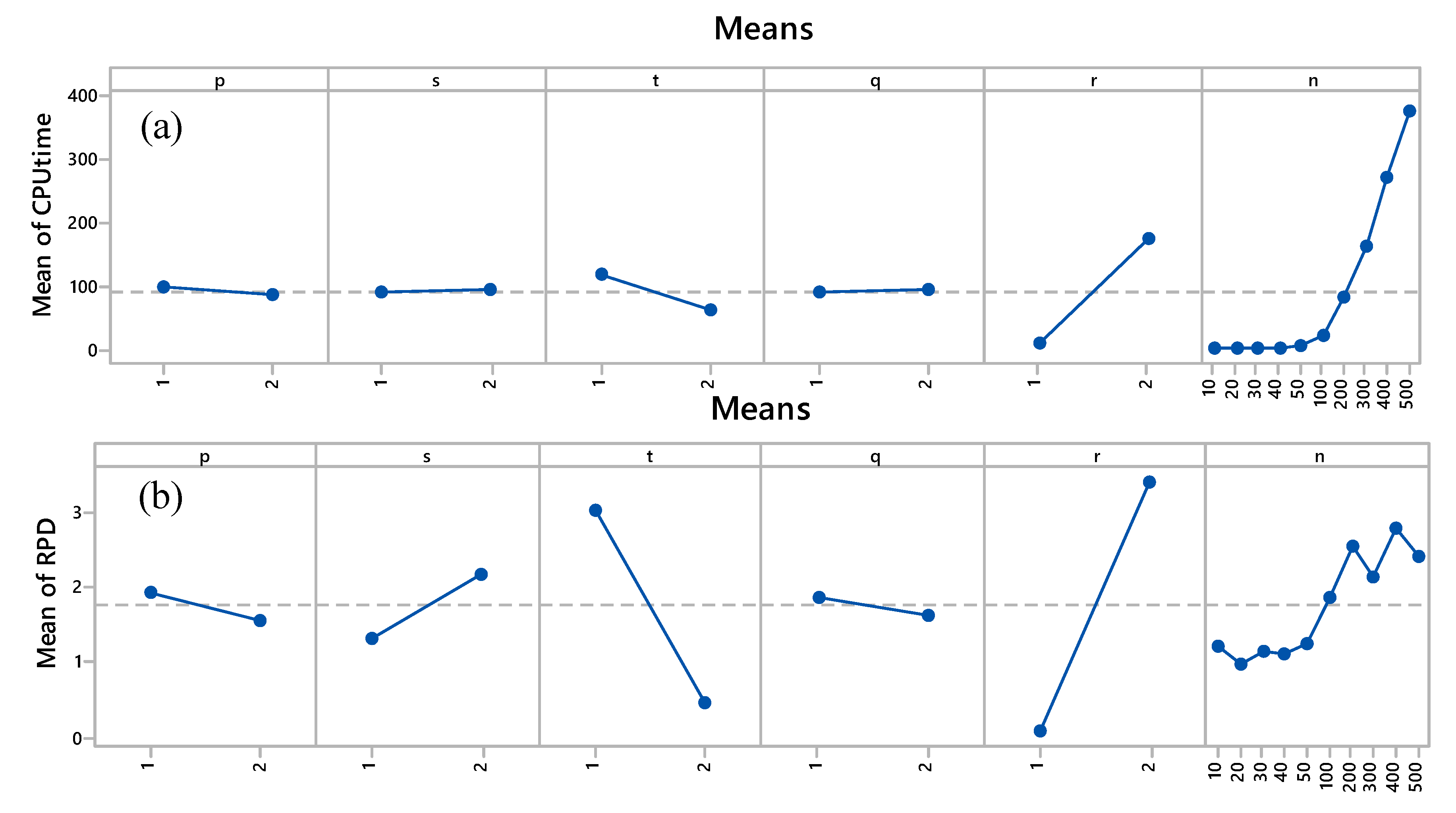
The computational results of the GA for the RPD and CPU times are given in Table 8 and Table 9, respectively. Results are also presented in Figure 3a–f. The following notations are used in Table 8, Table 9, and Figure 3:
- denotes the number of jobs.
- 1,2 refer to the low and high levels, respectively, corresponding to variables p, r, q, t, and s.
- RPD-1 and RPD-2 refer to the RPD at low and high levels, respectively, corresponding to variables p, r, q, t, and s.
- CPU-1 and CPU-2 refer to the CPU time at low and high levels, respectively, corresponding to variables p, r, q, t, and s.
Computational results of the RPD and CPU time are summarized in Table 8 and Table 9. It is evident from Table 8 that the release time factor has the most effect on the RPD. Increasing the release time interval from low level () to the high level () makes the problem very difficult to reach the LB and take high CPU time. The maximum error (RPD) at a low level of was 1.71%, while the error reaches 18.50% at a high level of . The maximum CPU time at a low level of was 55.7 seconds, while the CPU time reached 1113.9 seconds at a high level of . However, the RPD and CPU time are relatively reduced at a high level of when the availability period is high (). The CPU time is significantly increased with an increase in .
Figure 3a and Figure 4f show the effect of these variables on the average RPD and CPU time with the changes in the number of jobs. Figure 3a shows that an increase in the number of jobs increases the RPD and CPU time. Figure 3b shows the average RPD and CPU time at low and high variable. Moreover, there is no difference between them as the trends at low and high are very close to each other. Figure 3c shows a significant effect of the variable on the average RPD and CPU time. Figure 3d shows the average RPD and CPU time at low and high variable. Furthermore, there is no difference between them as the trends at low and high q are very close to each other. Figure 3e shows a significant effect of the variable on the average RPD. However, the effect of on the CPU time is significant at a high number of jobs.
The effects of these variables were also studied statistically using ANOVA. In this section, ANOVA analysis will be used to investigate the effect of five factors on each response. First, the ANOVA table for the CPU time has been presented. Table 10 shows the ANOVA table of the CPU time. Note that the CPU time data was transformed using Box-Cox transformation (square root) to meet normality assumption. After conducting a model fitting, it was revealed that a two-way interaction model is the best fit for the data. P-values less than 0.05 indicate model terms are significant. In this case, processing times (), release times (), availability period (), delivery times (), and sample sizes () are significant model terms. In other words, these factors significantly affect the transformed CPU time. P-values greater than 0.05 indicate that the model terms are not significant. Moreover, the interactions between the release times () and the processing times (), available period (), delivery times (), and sample sizes () have significant effects on the CPU times. This is also true for the interactions between the sample sizes () and the available period (). It is worth noting that the adjusted is equal to 98.17%, which indicates an excellent representation of the variability of the data by the model terms. Moreover, the contribution of the model is very high, since it is more than 98%. The most significant effects are contributed by changing the sample size () factor (48.47%), and then followed by the interaction between the release times () and the sample sizes () (25.01%). Release time () has a contribution of (20.65%).
Table 11 presents the ANOVA results for the RPD. It is worth noting that the data was transformed using square root transformation to meet the normality assumption. Since the used data are more than 300; the normality assumption has been verified using the values of skewness and kurtosis [59]. The results revealed that the processing times (p), unavailability period (s), available period (t), release times (r), and sample sizes (n) have a significant effect on the RPD, since their P-values are all less than 0.05. Consequently, the processing times (p), unavailability period (s), available period (t), release times (r), and sample sizes (n) have a significant effect on the quality of the solution obtained by the model. Moreover, the interactions between the processing times (p) and unavailability period (s); between processing times (p) and release times (r); between unavailability period (s) and available period (t); between unavailability period (s) and release times (r); between available period (t) and release times (r); between delivery times (q) and release times (r); and between release times (r) and sample sizes (n), all have a significant effect on the quality of the solution obtained by the model. This model has shown a good R2 value = 0.83, which indicates the data variability is more represented by the model. Moreover, the contribution of the model is high since it is more than 83%. However, changing the release times (r) (45.06%) and its interaction with availability times (t) (12.81%) contribute more effects.
Furthermore, the results have been visualized to represent the direction impacts of the factors and their interactions on the corresponding response. Figure 4 shows the main effects of the factors being studied on the RPD and CPU time. Figure 4a shows that the more the availability period (t), the less the CPU time needed for obtaining a good solution for the corresponding problem, regardless of the other factors. Furthermore, the first level of the release time factor (r) shows less CPU time. This is caused by the short period receiving orders in the first level of the release time factor. In addition, as it is shown, the greater the sample size, the more CPU time is needed. Moreover, Figure 4b shows that the processing time, availability period, and delivery time are inversely proportional to the RPD. However, the unavailability period, release time, and sample size are directly proportional to the RPD.
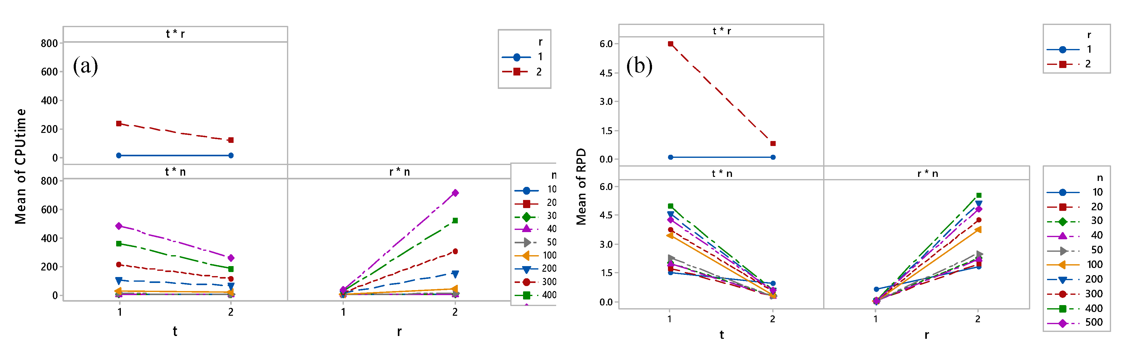
Moreover, the interaction plot of the factors that affect the RPD and CPU time are plotted in Figure 5. Figure 5a shows that there is a significant effect in the interaction between the availability period and release time in the CPU. Additionally, the more availability period and release time, the CPU time is less. Furthermore, the release time increases the CPU time with the increase in sample size. Figure 5b shows the interaction plot for the RPD. It is worth noting that almost the same interaction effects of the CPU times are applied to the RPD.
6. Conclusions
The scheduling problem of two identical parallel machines subjected to release times and delivery times, where the machines are periodically unavailable, is tackled in this study. The machines were assumed undergoing periodic maintenance instead of assuming they are always available. This makes the scheduling problem more practical. The objective is to schedule all jobs such that the is minimized. An LB was proposed for the problem. A GA was proposed to solve the problem, since the problem is considered an NP-hard problem. The GA performance was evaluated in terms of the RPD (the relative distance to the LB) and CPU time. For better performance of the GA, RSM was used to optimize the GA parameters, namely, population size (Popsize), crossover probability (Pc), mutation probability (Pm), mutation ratio (Mu), and pressure selection (Beta), while minimizing the RPD and CPU time. The optimization of multiple responses (RPD and CPU time) was performed using the desirability analysis. Optimized settings of the GA parameters were used to further evaluate the scheduling problem. Factorial design of the scheduling problem input variables, namely, processing times, release times, delivery times, availability and unavailability periods, and the number of jobs, was used to evaluate the GA performance.
The results show that the GA parameters have significant effects on the RPD and CPU time with R2 being equal to 90.14% and 82.45%, respectively. Furthermore, the GA parameter interactions have high contributions to the RPD and CPU time. To minimize the RPD and CPU time, the GA parameters should be set as follows: Popsize is 200, Pc is 0.9, Pm is 0.14, Mu is 0.001, and Beta is 1. Regarding the scheduling problem input variables, increasing the release time interval makes the problem very difficult to reach the LB. Moreover, increasing the release time interval leads to a significant increase in the CPU time when the number of jobs is high. Increasing the number of jobs leads to an increase in CPU time. Decreasing the availability periods leads to a significant increase in the RPD and CPU time when the number of jobs is greater than 50 jobs.
Release times and availability period variables and their interaction most affect the RPD. Finally, the most significant variables that affect the CPU time are release times and sample sizes and their interactions.
Author Contributions
Conceptualization, M.S.; Data curation, M.S. and M.A.; Funding acquisition, A.M.A.-S.; Investigation, A.M.A.-S., M.S., M.A. and M.G.; Methodology, A.M.A.-S., M.S. and M.A.; Resources, M.S. and M.G.; Supervision, A.M.A.-S. and M.S.; Validation, M.S.; Visualization, M.S. and M.A.; Writing—original draft, M.S. and M.A.; Writing—review & editing, A.M.A.-S., M.S., M.A. and M.G. All authors have read and agreed to the published version of the manuscript.
Funding
This research was funded by Vice Deanship of Scientific Research Chairs (DSRVCH) and the APC was funded by Vice Deanship of Scientific Research Chairs (DSRVCH).
Acknowledgments
The authors are grateful to the Deanship of Scientific Research, King Saud University for funding this research project through Vice Deanship of Scientific Research Chairs (DSRVCH) and the authors thank RSSU at King Saud University for their technical support.
Conflicts of Interest
The authors declare no conflict of interest.
References
- Pinedo, M.; Chao, X. Operations Scheduling with Applications in Manufacturing and Services; McGraw Hill: New York, NY, USA, 1999. [Google Scholar]
- Kerzner, H. Project Management: A Systems Approach to Planning, Scheduling, and Controlling; John Wiley & Sons: Hoboken, NJ, USA, 2017. [Google Scholar]
- Callahan, M.T.; Quackenbush, D.G.; Rowings, J.E. Construction Project Scheduling; McGraw-Hill: New York, NY, USA, 1992. [Google Scholar]
- Barnhart, C.; Cohn, A.M.; Johnson, E.L.; Klabjan, D.; Nemhauser, G.L.; Vance, P.H. Airline crew scheduling. In Handbook of Transportation Science; Kluwer’s International Series; Springer: New York, NY, USA, 2003; pp. 517–560. [Google Scholar]
- Kaandorp, G.C.; Koole, G. Optimal outpatient appointment scheduling. Health Care Manag. Sci. 2007, 10, 217–229. [Google Scholar] [CrossRef] [PubMed] [Green Version]
- Malik, M.A.K. Reliable preventive maintenance scheduling. AIIE Trans. 1979, 11, 221–228. [Google Scholar] [CrossRef]
- Liu, Y.; Xu, X.; Zhang, L.; Wang, L.; Zhong, R.Y. Workload-based multi-task scheduling in cloud manufacturing. Robot. Comput.-Integr. Manuf. 2017, 45, 3–20. [Google Scholar] [CrossRef]
- Porto, A.F.; Henao, C.A.; López-Ospina, H.; González, E.R. Hybrid flexibility strategy on personnel scheduling: Retail case study. Comput. Ind. Eng. 2019, 133, 220–230. [Google Scholar] [CrossRef]
- Pinedo, M. Scheduling: Theory, Algorithms, and Systems; Springer: New York, NY, USA, 2012; Volume 5. [Google Scholar]
- Abedinnia, H.; Glock, C.H.; Grosse, E.H.; Schneider, M. Machine scheduling problems in production: A tertiary study. Comput. Ind. Eng. 2017, 111, 403–416. [Google Scholar] [CrossRef]
- Cheng, T.; Sin, C. A state-of-the-art review of parallel-machine scheduling research. Eur. J. Oper. Res. 1990, 47, 271–292. [Google Scholar] [CrossRef]
- Wang, S.; Wu, R.; Chu, F.; Yu, J. Identical Parallel Machine Scheduling with Assurance of Maximum Waiting Time for an Emergency Job. Comput. Oper. Res. 2020, 104918. [Google Scholar] [CrossRef]
- Li, K.; Yang, S.-l. Non-identical parallel-machine scheduling research with minimizing total weighted completion times: Models, relaxations and algorithms. Appl. Math. Model. 2009, 33, 2145–2158. [Google Scholar] [CrossRef]
- Vallada, E.; Ruiz, R. A genetic algorithm for the unrelated parallel machine scheduling problem with sequence dependent setup times. Euro. J. Oper. Res. 2011, 211, 612–622. [Google Scholar] [CrossRef] [Green Version]
- Anand, S.; Bringmann, K.; Friedrich, T.; Garg, N.; Kumar, A. Minimizing maximum (weighted) flow-time on related and unrelated machines. Algorithmica 2017, 77, 515–536. [Google Scholar] [CrossRef] [Green Version]
- Wang, J.-Y. Minimizing the total weighted tardiness of overlapping jobs on parallel machines with a learning effect. J. Oper. Res. Soc. 2019, 71, 910–927. [Google Scholar] [CrossRef]
- Chaudhry, I.A.; Elbadawi, I.A. Minimisation of total tardiness for identical parallel machine scheduling using genetic algorithm. Sādhanā 2017, 42, 11–21. [Google Scholar] [CrossRef] [Green Version]
- Zheng, F.; Huang, J. Uniform parallel-machine scheduling to minimize the number of tardy jobs in the MapReduce system. In Proceedings of the 2019 International Conference on Industrial Engineering and Systems Management (IESM), Shanghai, China, 25–27 September 2019; pp. 1–6. [Google Scholar]
- Ozturk, O.; Begen, M.A.; Zaric, G.S. A branch and bound algorithm for scheduling unit size jobs on parallel batching machines to minimize makespan. Int. J. Prod. Res. 2017, 55, 1815–1831. [Google Scholar] [CrossRef]
- Martello, S.; Soumis, F.; Toth, P. Exact and approximation algorithms for makespan minimization on unrelated parallel machines. Discret. Appl. Math. 1997, 75, 169–188. [Google Scholar] [CrossRef] [Green Version]
- Mansouri, S.A.; Aktas, E.; Besikci, U. Green scheduling of a two-machine flowshop: Trade-off between makespan and energy consumption. Eur. J. Oper. Res. 2016, 248, 772–788. [Google Scholar] [CrossRef] [Green Version]
- Dao, T.-K.; Pan, T.-S.; Pan, J.-S. Parallel bat algorithm for optimizing makespan in job shop scheduling problems. J. Intell. Manuf. 2018, 29, 451–462. [Google Scholar] [CrossRef]
- Bai, D.; Zhang, Z.-H.; Zhang, Q. Flexible open shop scheduling problem to minimize makespan. Comput. Oper. Res. 2016, 67, 207–215. [Google Scholar] [CrossRef]
- Shabtay, D.; Zofi, M. Single machine scheduling with controllable processing times and an unavailability period to minimize the makespan. Int. J. Prod. Econ. 2018, 198, 191–200. [Google Scholar] [CrossRef]
- Hamzadayi, A.; Yildiz, G. Modeling and solving static m identical parallel machines scheduling problem with a common server and sequence dependent setup times. Comput. Ind. Eng. 2017, 106, 287–298. [Google Scholar] [CrossRef]
- Lee, C.-Y. Parallel machines scheduling with nonsimultaneous machine available time. Discret. Appl. Math. 1991, 30, 53–61. [Google Scholar] [CrossRef] [Green Version]
- Kaabi, J.; Harrath, Y. Scheduling on uniform parallel machines with periodic unavailability constraints. Int. J. Prod. Res. 2019, 57, 216–227. [Google Scholar] [CrossRef]
- Pfund, M.; Fowler, J.W.; Gadkari, A.; Chen, Y. Scheduling jobs on parallel machines with setup times and ready times. Comput. Ind. Eng. 2008, 54, 764–782. [Google Scholar] [CrossRef]
- Al-harkan, I.M.; Qamhan, A.A. Optimize Unrelated Parallel Machines Scheduling Problems With Multiple Limited Additional Resources, Sequence-Dependent Setup Times and Release Date Constraints. IEEE Access 2019, 7, 171533–171547. [Google Scholar] [CrossRef]
- Mensendiek, A.; Gupta, J.N. Scheduling Identical Parallel Machines with a Fixed Number of Delivery Dates. In Operations Research Proceedings 2014; Springer: Cham, Switzerland, 2016; pp. 393–398. [Google Scholar]
- Hermès, F.; Ghédira, K. Scheduling Jobs with Releases Dates and Delivery Times on M Identical Non-idling Machines. In Proceedings of the ICINCO (1), Madrid, Spain, 26–28 July 2017; pp. 82–91. [Google Scholar]
- Hidri, L.; Al-Samhan, A.M.; Mabkhot, M.M. Bounding Strategies for the Parallel Processors Scheduling Problem With No-Idle Time Constraint, Release Date, and Delivery Time. IEEE Access 2019, 7, 170392–170405. [Google Scholar] [CrossRef]
- Liu, P.; Gu, M.; Li, G. Two-agent scheduling on a single machine with release dates. Comput. Oper. Res. 2019, 111, 35–42. [Google Scholar] [CrossRef]
- Schutten, J.M.; Leussink, R. Parallel machine scheduling with release dates, due dates and family setup times. Int. J. Prod. Econ. 1996, 46, 119–125. [Google Scholar] [CrossRef] [Green Version]
- Timkovsky, V.G. A polynomial-time algorithm for the two-machine unit-time release-date job-shop schedule-length problem. Discret. Appl. Math. 1997, 77, 185–200. [Google Scholar] [CrossRef] [Green Version]
- Bai, D.; Tang, L. Open shop scheduling problem to minimize makespan with release dates. Appl. Math. Model. 2013, 37, 2008–2015. [Google Scholar] [CrossRef]
- Gharbi, A.; Haouari, M. An approximate decomposition algorithm for scheduling on parallel machines with heads and tails. Comput. Oper. Res. 2007, 34, 868–883. [Google Scholar] [CrossRef]
- Woeginger, G.J. Heuristics for parallel machine scheduling with delivery times. Acta Inform. 1994, 31, 503–512. [Google Scholar] [CrossRef]
- Mastrolilli, M. Efficient approximation schemes for scheduling problems with release dates and delivery times. J. Sched. 2003, 6, 521–531. [Google Scholar] [CrossRef]
- Kacem, I.; Kellerer, H. Approximation algorithms for no idle time scheduling on a single machine with release times and delivery times. Discret. Appl. Math. 2014, 164, 154–160. [Google Scholar] [CrossRef]
- Das, K.; Lashkari, R.; Sengupta, S. Machine reliability and preventive maintenance planning for cellular manufacturing systems. Eur. J. Oper. Res. 2007, 183, 162–180. [Google Scholar] [CrossRef]
- Liao, C.-J.; Shyur, D.-L.; Lin, C.-H. Makespan minimization for two parallel machines with an availability constraint. Eur. J. Oper. Res. 2005, 160, 445–456. [Google Scholar] [CrossRef]
- Xu, D.; Cheng, Z.; Yin, Y.; Li, H. Makespan minimization for two parallel machines scheduling with a periodic availability constraint. Comput. Oper. Res. 2009, 36, 1809–1812. [Google Scholar] [CrossRef]
- Liao, C.; Chen, C.; Lin, C. Minimizing makespan for two parallel machines with job limit on each availability interval. J. Oper. Res. Soc. 2007, 58, 938–947. [Google Scholar] [CrossRef]
- Lin, C.-H.; Liao, C.-J. Makespan minimization for two parallel machines with an unavailable period on each machine. Int. J. Adv. Manuf. Technol. 2007, 33, 1024–1030. [Google Scholar] [CrossRef]
- Liu, M.; Zheng, F.; Chu, C.; Xu, Y. Optimal algorithms for online scheduling on parallel machines to minimize the makespan with a periodic availability constraint. Theor. Comput. Sci. 2011, 412, 5225–5231. [Google Scholar] [CrossRef] [Green Version]
- Xu, D.; Yang, D.-L. Makespan minimization for two parallel machines scheduling with a periodic availability constraint: Mathematical programming model, average-case analysis, and anomalies. Appl. Math. Model. 2013, 37, 7561–7567. [Google Scholar] [CrossRef]
- Hashemian, N.; Diallo, C.; Vizvári, B. Makespan minimization for parallel machines scheduling with multiple availability constraints. Ann. Oper. Res. 2014, 213, 173–186. [Google Scholar] [CrossRef]
- Huo, Y. Parallel machine makespan minimization subject to machine availability and total completion time constraints. J. Sched. 2017, 1–15. [Google Scholar] [CrossRef]
- Huang, H.; Xiong, Y.; Zhou, Y. A larger pie or a larger slice? Contract negotiation in a closed-loop supply chain with remanufacturing. Comput. Ind. Eng. 2020, 142, 106377. [Google Scholar] [CrossRef]
- Carlier, J. Scheduling jobs with release dates and tails on identical machines to minimize the makespan. Eur. J. Oper. Res. 1987, 29, 298–306. [Google Scholar] [CrossRef]
- Low, C.; Ji, M.; Hsu, C.-J.; Su, C.-T. Minimizing the makespan in a single machine scheduling problems with flexible and periodic maintenance. Appl. Math. Model. 2010, 34, 334–342. [Google Scholar] [CrossRef]
- Kundakcı, N.; Kulak, O. Hybrid genetic algorithms for minimizing makespan in dynamic job shop scheduling problem. Comput. Ind. Eng. 2016, 96, 31–51. [Google Scholar] [CrossRef]
- Osaba, E.; Carballedo, R.; Diaz, F.; Onieva, E.; De La Iglesia, I.; Perallos, A. Crossover versus mutation: A comparative analysis of the evolutionary strategy of genetic algorithms applied to combinatorial optimization problems. Sci. World J. 2014, 2014, 1–22. [Google Scholar] [CrossRef] [Green Version]
- Goldberg, D. Genetic Algorithms in Search, Optimization, and Machine learning; Addison-Wesley Pub. Co.: Boston, MA, USA, 1989; ISBN 0201157675. [Google Scholar]
- Abreu, L.R.; Cunha, J.O.; Prata, B.A.; Framinan, J.M. A genetic algorithm for scheduling open shops with sequence-dependent setup times. Comput. Oper. Res. 2020, 113, 104793. [Google Scholar] [CrossRef]
- Syswerda, G. Scheduling optimization using genetic algorithms. In Handbook of Genetic Algorithms; Van Nostrand Reinhold: New York, NY, USA, 1991. [Google Scholar]
- Derringer, G.; Suich, R. Simultaneous optimization of several response variables. J. Qual. Technol. 1980, 12, 214–219. [Google Scholar] [CrossRef]
- Kim, H.-Y. Statistical notes for clinical researchers: Assessing normal distribution (2) using skewness and kurtosis. Restor. Dent. Endod. 2013, 38, 52–54. [Google Scholar] [CrossRef]
Figure 1.
Gantt chart of the example .

Figure 2.
Example of a position-based crossover (PBX) operator.

Figure 3.
Effects of variables (a) number of jobs, ; (b) processing times, ; (c) ready times, ; (d) delivery times, , (e) machine availability time, ; and (f) machine unavailability time, on the RPD and CPU time.
Figure 3.
Effects of variables (a) number of jobs, ; (b) processing times, ; (c) ready times, ; (d) delivery times, , (e) machine availability time, ; and (f) machine unavailability time, on the RPD and CPU time.

Figure 4.
Main effects of the factors being studied on (a) the CPU time and (b) PRD.

Figure 5.
Interaction plots for (a) the CPU time and (b) RPD.


Table 1.
Processing times, release times, and delivery times of the example.
| j | 1 | 2 | 3 | 4 | 5 | 6 | 7 | 8 |
| 1 | 1 | 2 | 4 | 2 | 3 | 1 | 2 | |
| 2 | 5 | 2 | 1 | 6 | 2 | 6 | 3 | |
| 3 | 5 | 7 | 4 | 6 | 4 | 4 | 2 |
Table 2.
Available and unavailable periods of machines 1 and 2 of the example.
| 9 | 2 |
Table 3.
Experimental characteristics of the generated instances.
| Input | Levels | |||||||||
|---|---|---|---|---|---|---|---|---|---|---|
| 1 | 2 | 3 | 4 | 5 | 6 | 7 | 8 | 9 | 10 | |
| p | U(20,50) | U(20,100) | ||||||||
| r | U(1,a) | U(1,) | ||||||||
| q | U(1,0.5b) | U(1,1.5b) | ||||||||
| t | ||||||||||
| s | ||||||||||
| n | 10 | 20 | 30 | 40 | 50 | 100 | 200 | 300 | 400 | 500 |
Table 4.
The genetic algorithm (GA) parameters and their respective levels.
| Parameter | −1 | 0 | 1 |
|---|---|---|---|
| Popsize | 20 | 210 | 400 |
| Pc | 0.1 | 0.695 | 0.99 |
| Pm | 0.1 | 0.5 | 0.9 |
| Mu | 0.001 | 0.1505 | 0.3 |
| Beta | 1 | 10 | 19 |
Table 5.
Reduced analysis of variance (ANOVA) table for the relative percentage deviation (RPD).
| Source | DF | Seq SS | Contribution | Adj SS | Adj MS | F-value | P-value |
|---|---|---|---|---|---|---|---|
| Model | 8 | 0.007765 | 90.14% | 0.007765 | 0.000971 | 49.16 | 0 |
| Linear | 4 | 0.006092 | 70.72% | 0.006092 | 0.001523 | 77.14 | 0 |
| Popsize | 1 | 0.005858 | 68.00% | 0.005858 | 0.005858 | 296.71 | 0 |
| Pm | 1 | 0 | 0.00% | 0 | 0 | 0.01 | 0.935 |
| Mu | 1 | 0.000131 | 1.52% | 0.000131 | 0.000131 | 6.61 | 0.014 |
| Beta | 1 | 0.000103 | 1.20% | 0.000103 | 0.000103 | 5.22 | 0.027 |
| Square | 1 | 0.00131 | 15.21% | 0.00131 | 0.00131 | 66.37 | 0 |
| Popsize2 | 1 | 0.00131 | 15.21% | 0.00131 | 0.00131 | 66.37 | 0 |
| Two-way interaction | 3 | 0.000363 | 4.21% | 0.000363 | 0.000121 | 6.13 | 0.001 |
| Popsize×Pm | 1 | 0.000229 | 2.66% | 0.000229 | 0.000229 | 11.61 | 0.001 |
| Popsize×Beta | 1 | 0.000091 | 1.06% | 0.000091 | 0.000091 | 4.6 | 0.038 |
| Pm×Mu | 1 | 0.000043 | 0.50% | 0.000043 | 0.000043 | 2.17 | 0.148 |
| Error | 43 | 0.000849 | 9.86% | 0.000849 | 0.00002 | ||
| Pure error | 9 | 0.00003 | 0.35% | 0.00003 | 0.000003 | ||
| Total | 51 | 0.008614 | 100.00% |
R-sq: 90.14%; R-sq(adj): 88.31%; R-sq(pred): 83.95%.
Table 6.
Reduced ANOVA table for the central processing unit (CPU) time.
| Source. | DF | Seq SS | Contribution | Adj SS | Adj MS | F-Value | p-Value |
|---|---|---|---|---|---|---|---|
| Model | 8 | 572,596 | 82.45% | 572,596 | 71,574 | 25.26 | 0 |
| Linear | 4 | 322,331 | 46.42% | 322,331 | 80,583 | 28.44 | 0 |
| Popsize | 1 | 102,731 | 14.79% | 102,731 | 102,731 | 36.25 | 0 |
| Pc | 1 | 4120 | 0.59% | 4120 | 4120 | 1.45 | 0.234 |
| Pm | 1 | 131,009 | 18.87% | 131,009 | 131,009 | 46.23 | 0 |
| Mu | 1 | 84,471 | 12.16% | 84,471 | 84,471 | 29.81 | 0 |
| Two-way interaction | 4 | 250,265 | 36.04% | 250,265 | 62,566 | 22.08 | 0 |
| Popsize×Pc | 1 | 3960 | 0.57% | 3960 | 3960 | 1.4 | 0.244 |
| Popsize×Pm | 1 | 92,875 | 13.37% | 92,875 | 92,875 | 32.77 | 0 |
| Popsize×Mu | 1 | 71,356 | 10.28% | 71,356 | 71,356 | 25.18 | 0 |
| Pm×Mu | 1 | 82,074 | 11.82% | 82,074 | 82,074 | 28.96 | 0 |
| Error | 43 | 121,852 | 17.55% | 121,852 | 2834 | ||
| Pure error | 9 | 2039 | 0.29% | 2039 | 227 | ||
| Total | 51 | 694,448 | 100.00% |
R-sq: 82.45%; R-sq(adj): 79.19%; R-sq(pred): 69.06%.
Table 7.
The optimal combination values of the GA parameters.
| GA Parameters | Popsize | Pc | Pm | Mu | Beta |
|---|---|---|---|---|---|
| Best Settings | 200 | 0.90 | 0.14 | 0.001 | 1 |
Table 8.
Computational results of the RPD.
| Input | n | |||||||||||||
|---|---|---|---|---|---|---|---|---|---|---|---|---|---|---|
| p | r | q | t | s | 10 | 20 | 30 | 40 | 50 | 100 | 200 | 200 | 400 | 500 |
| 1 | 1 | 1 | 1 | 1 | 0.1 | 0 | 0.05 | 0.03 | 0.01 | 0.002 | 0.003 | 0.0008 | 0.003 | 0.003 |
| 2 | 0.29 | 0.04 | 0.03 | 0 | 0 | 0.016 | 0 | 0.001 | 0.001 | 0.003 | ||||
| 2 | 1 | 0.72 | 0.01 | 0 | 0 | 0.02 | 0.001 | 0.005 | 0.001 | 0.003 | 0.001 | |||
| 2 | 0.11 | 0.01 | 0 | 0 | 0.03 | 0.002 | 0.003 | 0.001 | 0.004 | 0.002 | ||||
| 2 | 1 | 1 | 0.23 | 0 | 0.05 | 0.01 | 0.02 | 0.032 | 0.021 | 0.008 | 0.008 | 0.008 | ||
| 2 | 1.11 | 0 | 0.01 | 0.01 | 0.05 | 0.012 | 0.014 | 0.008 | 0.013 | 0.008 | ||||
| 2 | 1 | 0.91 | 0.1 | 0.02 | 0.03 | 0.01 | 0.018 | 0.011 | 0.013 | 0.009 | 0.004 | |||
| 2 | 1 | 0.37 | 0 | 0.02 | 0.04 | 0.018 | 0.025 | 0.011 | 0.008 | 0.007 | ||||
| 2 | 1 | 1 | 1 | 2.51 | 3.51 | 7 | 7.46 | 3.37 | 0.592 | 16.34 | 11.48 | 5.827 | 2.464 | |
| 2 | 4.45 | 7.08 | 4.64 | 2.73 | 3.26 | 5.592 | 5.531 | 4.789 | 16.41 | 13.79 | ||||
| 2 | 1 | 0 | 1.66 | 0.39 | 0.3 | 1.89 | 0.905 | 1.692 | 1.2 | 1.519 | 1.717 | |||
| 2 | 4.95 | 0.19 | 0.28 | 0.89 | 0.87 | 1.536 | 1.916 | 2.104 | 1.989 | 1.754 | ||||
| 2 | 1 | 1 | 2.03 | 2.08 | 0.47 | 3.3 | 7.76 | 13.02 | 14.28 | 8.618 | 7.224 | 5.802 | ||
| 2 | 3.9 | 2.94 | 3.93 | 3.79 | 7.59 | 12.28 | 5.342 | 8.06 | 7.597 | 10.45 | ||||
| 2 | 1 | 0 | 0.15 | 0.11 | 0.16 | 0.27 | 0.541 | 1.234 | 1.184 | 2.002 | 1.592 | |||
| 2 | 0.26 | 0.29 | 0.25 | 0.79 | 0.11 | 1.059 | 1.448 | 1.503 | 1.626 | 1.583 | ||||
| 2 | 1 | 1 | 1 | 1 | 0.54 | 0 | 0 | 0.03 | 0.01 | 0.013 | 0.004 | 0.001 | 0.008 | 0.002 |
| 2 | 0.4 | 0.03 | 0.02 | 0.01 | 0.02 | 0.005 | 0.002 | 0.005 | 0.002 | 0.004 | ||||
| 2 | 1 | 0.63 | 0 | 0.05 | 0.01 | 0.02 | 0.011 | 0.015 | 0.002 | 0.004 | 0.003 | |||
| 2 | 0 | 0 | 0.01 | 0.02 | 0.02 | 0.007 | 0.007 | 0.005 | 0.003 | 0.002 | ||||
| 2 | 1 | 1 | 1.71 | 0.02 | 0.02 | 0.02 | 0.05 | 0.031 | 0.017 | 0.011 | 0.013 | 0.01 | ||
| 2 | 0.82 | 0.18 | 0.04 | 0.01 | 0.03 | 0.022 | 0.017 | 0.012 | 0.007 | 0.01 | ||||
| 2 | 1 | 0.86 | 0 | 0.04 | 0.03 | 0.02 | 0.031 | 0.022 | 0.018 | 0.017 | 0.007 | |||
| 2 | 0.75 | 0.05 | 0 | 0.04 | 0.02 | 0.023 | 0.022 | 0.019 | 0.008 | 0.008 | ||||
| 2 | 1 | 1 | 1 | 2.07 | 0.9 | 2.67 | 1.93 | 0.59 | 2.327 | 3.921 | 3.449 | 3.781 | 6.719 | |
| 2 | 2.25 | 5.29 | 3.6 | 4.07 | 3.47 | 17.65 | 15.41 | 10.71 | 18.5 | 14.65 | ||||
| 2 | 1 | 0.35 | 0.59 | 2.45 | 0.64 | 0 | 0.102 | 0.451 | 0.442 | 0.695 | 0.537 | |||
| 2 | 2.98 | 0.89 | 0.87 | 0.54 | 0.62 | 0.376 | 0.963 | 0.555 | 0.828 | 0.537 | ||||
| 2 | 1 | 1 | 1.3 | 0.02 | 3.03 | 0.43 | 0.22 | 2.253 | 2.666 | 3.132 | 6.514 | 3.623 | ||
| 2 | 0.47 | 5.27 | 6.16 | 7.39 | 9.57 | 1.011 | 9.588 | 9.407 | 13.65 | 10.79 | ||||
| 2 | 1 | 1.57 | 0 | 0 | 0.07 | 0.14 | 0.082 | 0.515 | 1.029 | 0.462 | 0.741 | |||
| 2 | 0 | 0.02 | 0.24 | 0.63 | 0.06 | 0.394 | 0.517 | 0.453 | 0.333 | 0.614 | ||||
Table 9.
Computational results of the CPU time.
| Input | n | |||||||||||||
|---|---|---|---|---|---|---|---|---|---|---|---|---|---|---|
| p | r | q | t | s | 10 | 20 | 30 | 40 | 50 | 100 | 200 | 200 | 400 | 500 |
| 1 | 1 | 1 | 1 | 1 | 2.1 | 0.6 | 3.6 | 3.5 | 2.3 | 2.9 | 6.2 | 5.1 | 15.0 | 20.2 |
| 2 | 3.8 | 2.5 | 2.3 | 0.5 | 1.8 | 6.1 | 2.8 | 5.7 | 10.5 | 23.6 | ||||
| 2 | 1 | 7.2 | 0.7 | 0.5 | 0.6 | 2.8 | 2.8 | 7.6 | 6.1 | 15.1 | 10.2 | |||
| 2 | 2.5 | 0.8 | 0.6 | 1.0 | 4.6 | 2.5 | 6.0 | 7.1 | 18.6 | 18.9 | ||||
| 2 | 1 | 1 | 3.4 | 0.3 | 3.2 | 2.9 | 3.9 | 7.2 | 16.6 | 15.6 | 28.5 | 37.9 | ||
| 2 | 6.1 | 0.5 | 1.8 | 2.7 | 6.2 | 7.6 | 17.7 | 17.6 | 31.1 | 34.6 | ||||
| 2 | 1 | 7.7 | 3.7 | 2.3 | 3.2 | 2.3 | 5.8 | 14.1 | 22.4 | 26.7 | 23.3 | |||
| 2 | 6.0 | 4.3 | 0.9 | 2.3 | 5.6 | 6.9 | 24.7 | 21.1 | 23.6 | 31.6 | ||||
| 2 | 1 | 1 | 1 | 3.9 | 8.7 | 13.8 | 15.7 | 18.3 | 47.2 | 204.6 | 368.1 | 746.3 | 962.6 | |
| 2 | 5.2 | 12.9 | 8.5 | 12.6 | 18.4 | 71.7 | 274.5 | 440.5 | 561.6 | 1113.9 | ||||
| 2 | 1 | 0.1 | 6.4 | 7.5 | 5.1 | 10.8 | 31.4 | 139.0 | 231.3 | 333.2 | 530.7 | |||
| 2 | 7.4 | 2.3 | 7.3 | 9.7 | 13.1 | 43.7 | 143.4 | 239.2 | 404.6 | 565.5 | ||||
| 2 | 1 | 1 | 5.5 | 7.8 | 6.6 | 13.5 | 27.6 | 48.6 | 223.7 | 501.0 | 793.0 | 1057.9 | ||
| 2 | 7.4 | 8.3 | 12.6 | 13.7 | 24.9 | 75.9 | 243.1 | 370.2 | 794.5 | 1008.9 | ||||
| 2 | 1 | 0.1 | 2.6 | 2.1 | 5.1 | 4.2 | 32.7 | 148.2 | 200.3 | 369.2 | 519.3 | |||
| 2 | 1.9 | 2.2 | 4.0 | 7.8 | 7.7 | 32.9 | 125.5 | 239.9 | 400.2 | 534.1 | ||||
| 2 | 1 | 1 | 1 | 1 | 6.5 | 1.0 | 0.7 | 3.3 | 4.5 | 9.2 | 11.3 | 10.7 | 31.7 | 28.3 |
| 2 | 3.4 | 3.1 | 4.6 | 2.8 | 5.3 | 4.5 | 9.2 | 22.9 | 15.6 | 36.2 | ||||
| 2 | 1 | 6.3 | 0.8 | 5.3 | 1.4 | 4.4 | 8.9 | 22.1 | 12.0 | 22.3 | 29.7 | |||
| 2 | 0.2 | 0.4 | 1.9 | 4.0 | 4.6 | 6.4 | 15.9 | 19.8 | 22.3 | 27.7 | ||||
| 2 | 1 | 1 | 7.7 | 2.1 | 2.4 | 3.4 | 4.1 | 13.4 | 17.2 | 32.4 | 50.3 | 55.7 | ||
| 2 | 8.7 | 9.4 | 2.3 | 3.2 | 4.0 | 11.7 | 20.8 | 30.0 | 38.3 | 49.9 | ||||
| 2 | 1 | 7.9 | 1.3 | 4.1 | 3.6 | 4.0 | 12.7 | 25.2 | 30.6 | 44.6 | 46.5 | |||
| 2 | 8.1 | 2.7 | 0.8 | 5.6 | 3.5 | 11.2 | 23.5 | 37.2 | 36.8 | 48.0 | ||||
| 2 | 1 | 1 | 1 | 5.2 | 2.4 | 5.0 | 8.3 | 11.4 | 42.7 | 154.5 | 404.9 | 666.9 | 779.8 | |
| 2 | 5.1 | 7.1 | 7.8 | 15.6 | 12.2 | 46.5 | 142.3 | 438.2 | 743.7 | 983.5 | ||||
| 2 | 1 | 1.6 | 3.7 | 6.6 | 5.6 | 0.4 | 17.1 | 65.3 | 167.5 | 316.1 | 452.3 | |||
| 2 | 3.6 | 2.0 | 4.9 | 4.4 | 4.7 | 27.7 | 106.1 | 188.8 | 376.8 | 383.2 | ||||
| 2 | 1 | 1 | 1.6 | 2.0 | 9.0 | 5.1 | 7.5 | 50.3 | 161.4 | 308.2 | 595.2 | 845.2 | ||
| 2 | 1.8 | 8.9 | 13.7 | 9.9 | 22.7 | 65.4 | 156.9 | 394.6 | 653.8 | 744.8 | ||||
| 2 | 1 | 2.0 | 0.1 | 0.2 | 2.7 | 8.0 | 13.9 | 93.2 | 244.0 | 318.0 | 522.8 | |||
| 2 | 0.1 | 1.9 | 2.5 | 3.5 | 2.4 | 22.8 | 81.7 | 174.3 | 263.6 | 455.4 | ||||
Table 10.
ANOVA for the CPU time.
| Source | DF | Seq SS | Contribution | Adj SS | Adj MS | F-Value | p-Value |
|---|---|---|---|---|---|---|---|
| Model | 35 | 17,129.5 | 98.17% | 17,129.5 | 489.41 | 435.05 | 0 |
| Linear | 14 | 12,301.4 | 70.50% | 12,301.4 | 878.67 | 781.07 | 0 |
| p | 1 | 4.5 | 0.03% | 4.5 | 4.54 | 4.03 | 0.046 |
| s | 1 | 3.2 | 0.02% | 3.2 | 3.18 | 2.82 | 0.094 |
| t | 1 | 223.1 | 1.28% | 223.1 | 223.09 | 198.31 | 0 |
| q | 1 | 10.7 | 0.06% | 10.7 | 10.68 | 9.49 | 0.002 |
| r | 1 | 3603.2 | 20.65% | 3603.2 | 3603.24 | 3202.97 | 0 |
| n | 9 | 8456.7 | 48.47% | 8456.7 | 939.63 | 835.25 | 0 |
| 2-Way Interactions | 21 | 4828 | 27.67% | 4828 | 229.91 | 204.37 | 0 |
| 1 | 71 | 0.41% | 71 | 71.03 | 63.14 | 0 | |
| 1 | 214.8 | 1.23% | 214.8 | 214.8 | 190.94 | 0 | |
| 9 | 155.8 | 0.89% | 155.8 | 17.31 | 15.39 | 0 | |
| 1 | 21.7 | 0.12% | 21.7 | 21.67 | 19.26 | 0 | |
| 9 | 4364.7 | 25.01% | 4364.7 | 484.97 | 431.1 | 0 | |
| Error | 284 | 319.5 | 1.83% | 319.5 | 1.12 | ||
| Total | 319 | 17,448.9 | 100.00% |
Table 11.
ANOVA for the RPD.
| Source | DF | Seq SS | Contribution | Adj SS | Adj MS | F-Value | p-Value |
|---|---|---|---|---|---|---|---|
| Model | 29 | 273.925 | 83.35% | 273.925 | 9.446 | 50.06 | 0 |
| Linear | 14 | 203.531 | 61.93% | 203.531 | 14.538 | 77.05 | 0 |
| p | 1 | 1.509 | 0.46% | 1.509 | 1.509 | 8 | 0.005 |
| s | 1 | 3.459 | 1.05% | 3.459 | 3.459 | 18.33 | 0 |
| t | 1 | 42.627 | 12.97% | 42.627 | 42.627 | 225.91 | 0 |
| q | 1 | 0.254 | 0.08% | 0.254 | 0.254 | 1.35 | 0.247 |
| r | 1 | 148.072 | 45.06% | 148.072 | 148.072 | 784.73 | 0 |
| n | 9 | 7.61 | 2.32% | 7.61 | 0.846 | 4.48 | 0 |
| 2-Way Interactions | 15 | 70.395 | 21.42% | 70.395 | 4.693 | 24.87 | 0 |
| 1 | 0.995 | 0.30% | 0.995 | 0.995 | 5.27 | 0.022 | |
| 1 | 1.932 | 0.59% | 1.932 | 1.932 | 10.24 | 0.002 | |
| 1 | 1.896 | 0.58% | 1.896 | 1.896 | 10.05 | 0.002 | |
| 1 | 3.768 | 1.15% | 3.768 | 3.768 | 19.97 | 0 | |
| 1 | 42.091 | 12.81% | 42.091 | 42.091 | 223.07 | 0 | |
| 1 | 1.87 | 0.57% | 1.87 | 1.87 | 9.91 | 0.002 | |
| 9 | 17.843 | 5.43% | 17.843 | 1.983 | 10.51 | 0 | |
| Error | 290 | 54.721 | 16.65% | 54.721 | 0.189 | ||
| Total | 319 | 328.646 | 100.00% |
© 2020 by the authors. Licensee MDPI, Basel, Switzerland. This article is an open access article distributed under the terms and conditions of the Creative Commons Attribution (CC BY) license (http://creativecommons.org/licenses/by/4.0/).
Share and Cite
MDPI and ACS Style
Al-Shayea, A.M.; Saleh, M.; Alatefi, M.; Ghaleb, M. Scheduling Two Identical Parallel Machines Subjected to Release Times, Delivery Times and Unavailability Constraints. Processes 2020, 8, 1025. https://doi.org/10.3390/pr8091025
AMA Style
Al-Shayea AM, Saleh M, Alatefi M, Ghaleb M. Scheduling Two Identical Parallel Machines Subjected to Release Times, Delivery Times and Unavailability Constraints. Processes. 2020; 8(9):1025. https://doi.org/10.3390/pr8091025
Chicago/Turabian StyleAl-Shayea, Adel M., Mustafa Saleh, Moath Alatefi, and Mageed Ghaleb. 2020. "Scheduling Two Identical Parallel Machines Subjected to Release Times, Delivery Times and Unavailability Constraints" Processes 8, no. 9: 1025. https://doi.org/10.3390/pr8091025
Note that from the first issue of 2016, this journal uses article numbers instead of page numbers. See further details here.