Interfacial Thermal Conductivity and Its Anisotropy


1
Department of Chemical and Biological Engineering, Illinois Institute of Technology, Chicago, IL 60616, USA
2
Department of Chemical Engineering, University of Illinois at Chicago, Chicago, IL 60607, USA
*
Author to whom correspondence should be addressed.
Processes 2020, 8(1), 27; https://doi.org/10.3390/pr8010027
Submission received: 25 November 2019
/
Revised: 17 December 2019
/
Accepted: 20 December 2019
/
Published: 24 December 2019
(This article belongs to the Special Issue Feature Review Papers)
Abstract
:There is a significant effort in miniaturizing nanodevices, such as semi-conductors, currently underway. However, a major challenge that is a significant bottleneck is dissipating heat generated in these energy-intensive nanodevices. In addition to being a serious operational concern (high temperatures can interfere with their efficient operation), it is a serious safety concern, as has been documented in recent reports of explosions resulting from many such overheated devices. A significant barrier to heat dissipation is the interfacial films present in these nanodevices. These interfacial films generally are not an issue in macro-devices. The research presented in this paper was an attempt to understand these interfacial resistances at the molecular level, and present possibilities for enhancing the heat dissipation rates in interfaces. We demonstrated that the thermal resistances of these interfaces were strongly anisotropic; i.e., the resistance parallel to the interface was significantly smaller than the resistance perpendicular to the interface. While the latter is well-known—usually referred to as Kapitza resistance—the anisotropy and the parallel component have previously been investigated only for solid-solid interfaces. We used molecular dynamics simulations to investigate the density profiles at the interface as a function of temperature and temperature gradient, to reveal the underlying physics of the anisotropy of thermal conductivity at solid-liquid, liquid-liquid, and solid-solid interfaces.
1. Introduction
Experimental studies of interfacial thermal resistance are rather challenging. In macro-systems, the thermal resistance of the bulk phase completely overwhelms any interface effects, which become essentially negligible. On the other hand, the interfacial rather than the bulk thermal resistance is of greater interest and experimentally measurable (albeit with some effort) in nano-systems. There is an increasing need for further miniaturization of electronic components. To enable such miniaturization, it is necessary to efficiently dissipate the heat generated in these devices; since they are rather power-intensive, overheating can severely affect their functionality and is also a significant safety concern. Traditional designs to facilitate heat dissipation include the incorporation of nano-fins and nano-channels, which increase the contact area between the heat generator and the dissipating medium (usually a fluid). However, the thermal resistance associated with the solid-fluid interface is a significant barrier to heat transfer [1,2,3,4]. In a recent publication [5], we reported that the thermal resistance of the solid-fluid interface exhibited significant anisotropy. This anisotropy has theoretical and applied significance. The anisotropy in the thermal resistance offers the possibility of overcoming this interfacial barrier by directing heat dissipation along the direction of least thermal resistance. Previous studies on the anisotropy of interfacial thermal resistance have generally focused on solid-solid interfaces. Suleiman et al. [6] studied the anisotropic thermal resistance of wood and developed a model based on its layer structure. Other studies have investigated the anisotropy of layered-structure-materials, such as graphene, crystals, and polymers [7,8,9]. These materials are of interest because they are widely used to conduct heat or electricity. Cross-plane and in-plane thermal resistance of graphene oxide films under high-temperatures were investigated by Renteria et al. [10], and a significant anisotropy was found. The anisotropic in-plane thermal resistance of suspended layered black phosphorus was measured by Luo et al. using micro-Raman spectroscopy [11]. Other studies of crystals, such as diamond, Bi2Sr2CaCu2O8, Bi2Te3/Sb2Te3, etc., have also been reported [12,13,14]. In these experimental studies, the solids investigated usually have regular and repeatable structures. Anisotropy of liquid-solid interfacial layers has not been investigated except for some studies on liquid crystals [15,16,17]. Interfacial properties between two immiscible liquids are also very important for industrial processes, such as extraction, which is an efficient way to separate or remove substances from one phase to the other. Thermal properties are even more important when the system is sensitive to heat, as in applications to the separation of drugs that can lose their potency [18]. Although much work has been done to derive the thermal conductivities of emulsions from Fourier’s Law (Resistance = −∇T/Heat flux) assuming a serial structure [19], those equations are confined to a macroscopic view and have limitations when applied to the molecular level.
Molecular dynamics (MD) is an ideal tool for investigating interfacial thermal resistances. Computational and theoretical studies have many advantages over experiments: first, they do not require the actual manufacturing of nano-devices which can be challenging in itself; second, computational studies involve a small fraction of the cost of experiments; additionally, these studies can be carried out at extreme operating conditions, such as high temperature and high pressure; and finally, they offer molecular-level understanding of the phenomena involved [20,21]. Sofos et al. [22] reported anisotropy and non-homogeneity of liquid argon flowing through a nanochannel by using non-equilibrium molecular dynamics (NEMD) simulations. Similarly, Liu et al. [23] explored the thermal conductivity and shear viscosity of water inside single-walled carbon nanotubes using MD simulations. Comparisons of results from traditional NEMD [24] or reverse non-equilibrium MD (rNEMD) [25] and Green-Kubo [26,27] methods against experiments using common solvents have shown the reliability of molecular dynamics simulations.
In the first part of this paper, we have reviewed our previous studies on solid-liquid, liquid-liquid, and solid-solid interfacial properties. In the second part, following up on our previous study, we have demonstrated that the thermal resistance of these interfaces is strongly anisotropic, with the resistance parallel to the interface being significantly smaller than the more well-known perpendicular to the surface resistance, usually referred to as Kapitza resistance [5]. To understand the underlying physics responsible for the observed anisotropy of the interfacial thermal resistance, we extended our previous studies by examining the density profiles at the interface as it is affected by the temperature and the temperature gradient. We used molecular dynamics to prove that such anisotropy is not unique to the solid-liquid interface; it also occurs at liquid-liquid and solid-solid interfaces.
2. Methodology Used to Study the Interfacial Thermal Conductivity
2.1. Solid-Liquid Interface System Set-Up
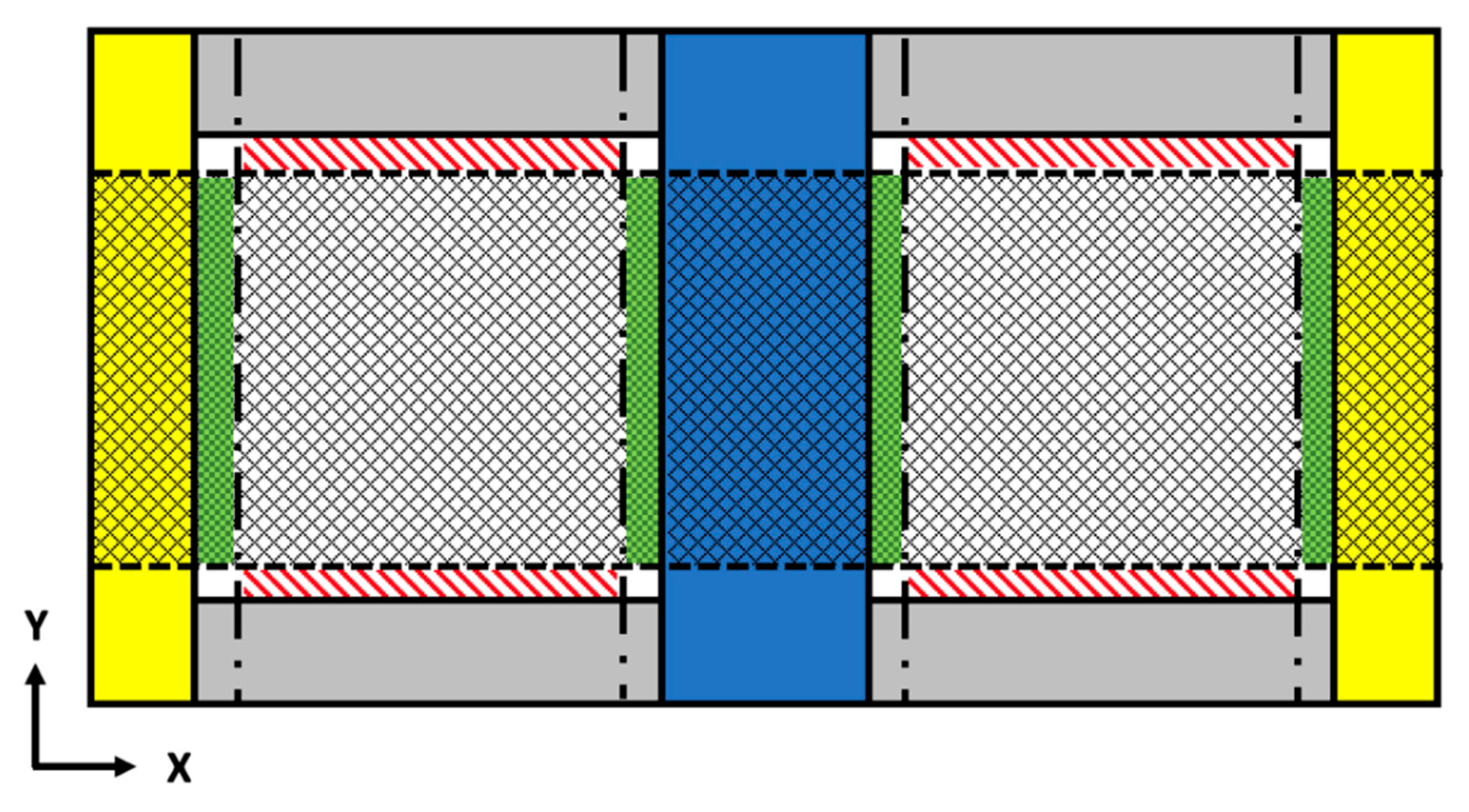
The simulation system should consider two thermal transport directions: across (perpendicular) or along (parallel) the solid-fluid interfaces. The walls can, in general, only impact a thin interfacial region, while the remaining fluid in the reservoirs continues to exhibit bulk properties. We designed a system where we could use molecular dynamics (MD) to explore the thermal transport in both the perpendicular and parallel directions to the solid-liquid interface. We investigated three working fluids confined within copper walls [5]. This special design also facilitated the equilibration by increasing interfacial surface area, which had been documented in our previous studies [28,29,30,31], and proved effective in investigating solid-fluid interfacial thermal conductivities [2,3,4]. Figure 1 shows a schematic sketch of a system set-up with a size of 130.14 × 65.07 × 28.92 Å in the x, y, z dimensions, respectively, that contains a liquid between solid walls. Our previous studies [2,3,4] have indicated that such a system size no longer has any size-dependent issues. Copper walls were represented by yellow, blue, and gray sections of 10.845 Å, 21.69 Å, and 10.845 Å thicknesses, respectively. The yellow walls were maintained at higher temperatures than those colored blue. By enforcing periodic boundary conditions, the two hot yellow walls Λh, in effect, constituted a single continuous wall of the same thickness as the colder blue wall Λc. The liquid was confined between these walls; as a result, the system generated several distinct solid-liquid stationary interfaces, which resulted in well-defined liquid density profiles [18]. This unique set-up allowed us to examine the thermal resistance in both the perpendicular and parallel directions to the interfaces simultaneously in a single simulation. The molar densities of the liquids required us to populate the volume between the system walls with 3400 water, or 1500 methanol, or 800 benzene molecules. Of these, water and methanol are polar, whereas benzene is nonpolar. The copper walls (yellow, blue, and grey) contained 11,520 copper atoms arranged in an FCC (Face Centered Cube) structure.
2.2. Liquid-Liquid Interface System Set-Up
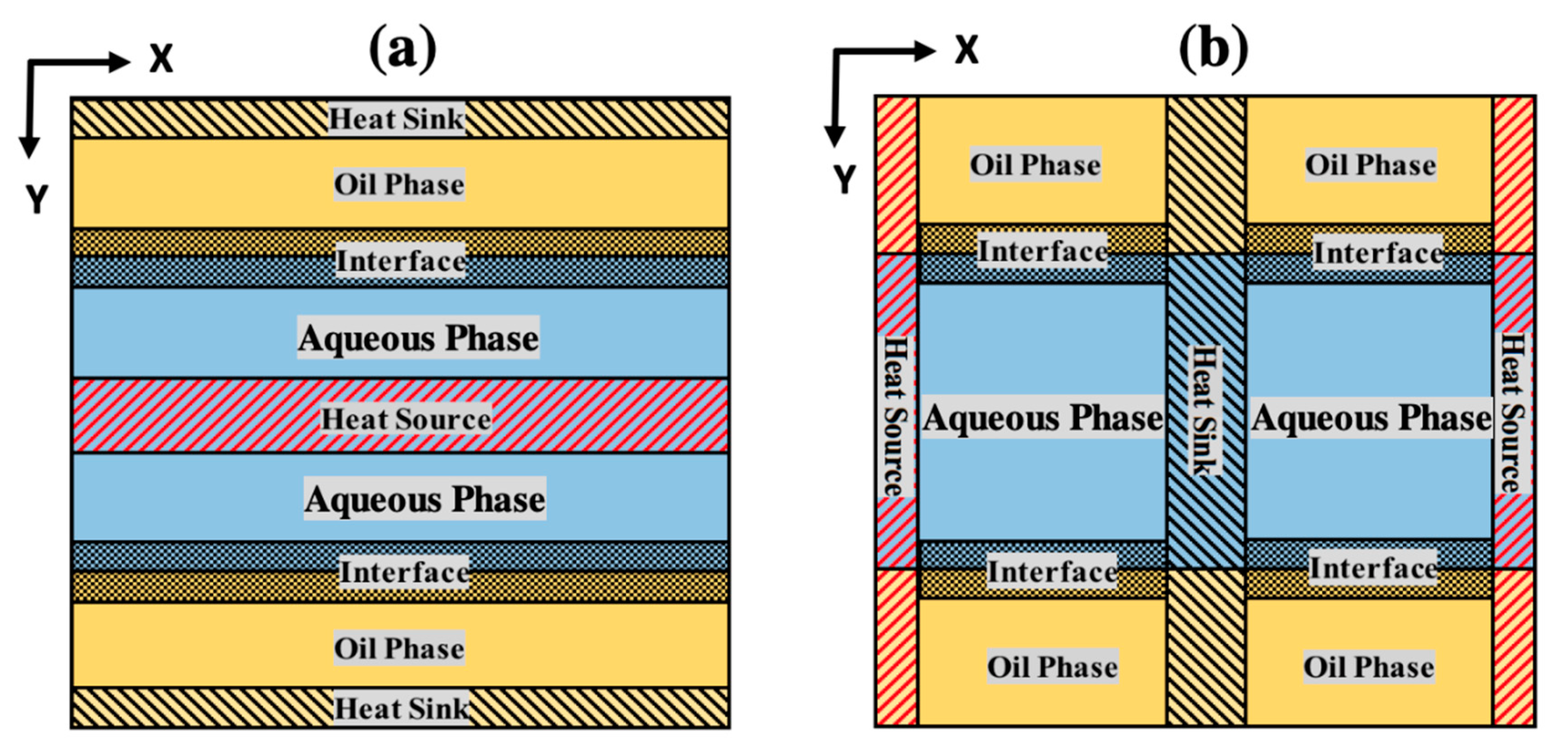
Figure 2a,b shows the system arrangements we used to study the liquid-liquid interface. This arrangement was different from the system set-up we used in the solid-liquid interface study; we removed the walls since an immiscible interface could be ensured based on our previous study of liquid-liquid equilibrium [18]. Although we used the word “oil” to describe the non-aqueous phase, it referred to a broad range of solvents other than water, including chloroform, carbon tetrachloride, and cyclo-/n-hexane. Since the system provided two independent measurements for two symmetric sections in one direction, the simulation error could also be estimated. The number of molecules used in the simulation corresponded to the experimental density data under ambient conditions (oil phase: 774 CCl4, 896 CHCl3, 660 cyclohexane, or 548 n-hexane; aqueous phase: 3828 water). We picked chloroform and carbon tetrachloride to examine the effect of polarity since they have similar sizes but different polarities. Cyclohexane and linear hexane were chosen to examine the effect of the molecular structure since they are non-polar molecules but have different structures.
2.3. Solid-Solid Interface System Set-Up
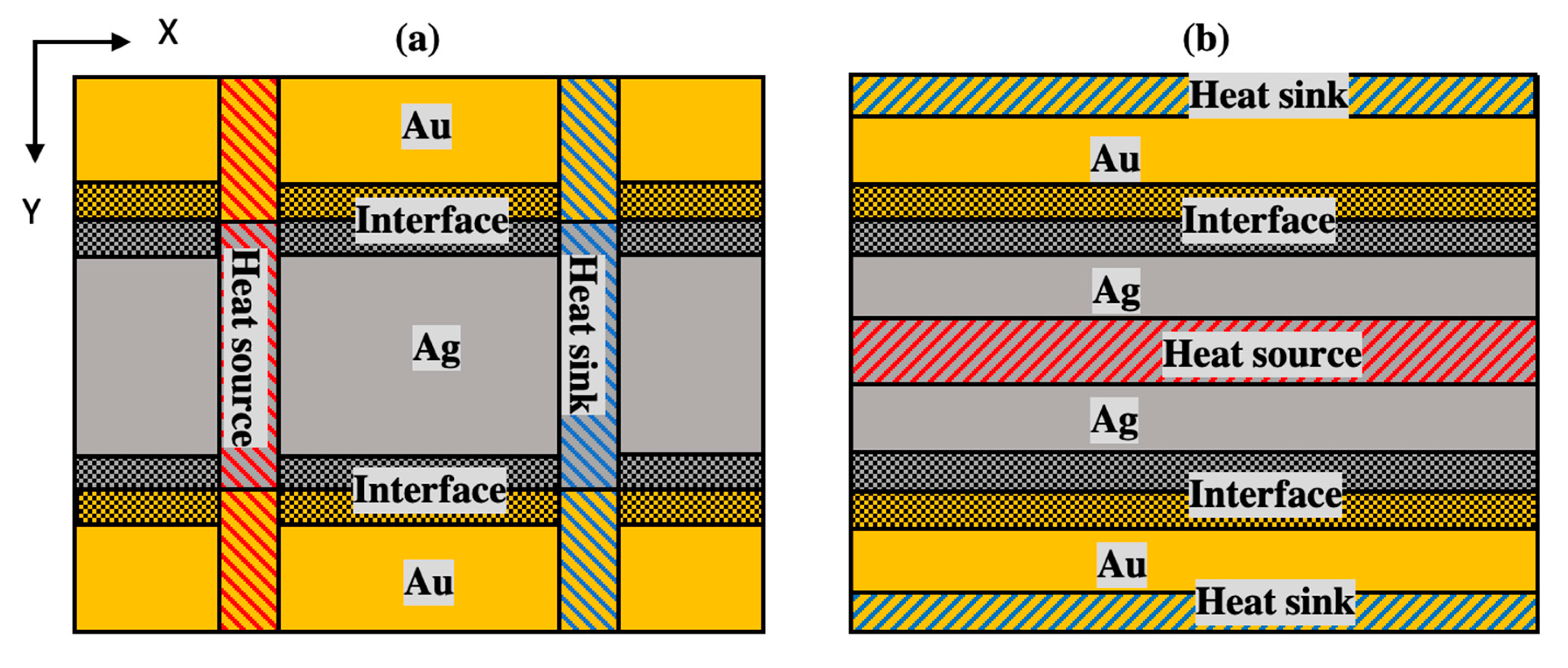
Figure 3a,b presents the system set-up we used to study solid-solid interfacial thermal conductivity. This set-up was similar to Figure 2 with the difference that we replaced the two liquid compartments by solid compartments, (gold or silver). The two gold slabs consisted of a total of 6912 atoms arranged in the FCC structure, and the silver slabs were likewise 6912.
2.4. Models Used and Simulation Procedures
For water, a TIP3P potential model was used [32], for copper, gold, and silver atoms, we used the EAM model [33], while for all other fluids (CCl4, CHCl3, cyclohexane, n-hexane, methanol, benzene), the Jorgensen United Atom OPLS force field [34,35] was used. The Lennard–Jones (LJ) 12–6 potential models’ cross terms were estimated using standard mixing rules. For the cross term between copper and liquid molecules, copper atoms were treated as LJ particles [36]. To estimate long-range electrostatic forces and energies, a particle-particle particle-mesh solver [37] was used, which was computationally more efficient while being as reliable as the traditional Ewald technique.
We examined the thermal transport parallel and perpendicular to the red (δ||) and green (δ⊥) interfaces of Figure 1, respectively, and all regions labeled as “interface” in Figure 2 and Figure 3. In Figure 1, heat transfer from the hot copper walls (Λh) to the cold copper wall Λc occurred perpendicular to the green interfacial layer (Λ⊥), while it proceeded parallel to the red interfacial layer (δ||) along the gray wall (Λa). To estimate the thermal conductivity κ⊥ perpendicular to the interface, we monitored the heat added to Λh in the yellow hatched area of Figure 1 and the heat removed from the corresponding blue hatched area for Λc. Using the standard Fourier equation, (Resistance = ∇T), the temperature change across δ⊥, together with the surface area for heat transfer, enabled estimation of κ⊥. Similarly, the thermal conductivity κ|| of δ|| was calculated using the gradient of temperature along the interface (shown by red diagonal lines in Figure 1) and the heat added and removed from the corresponding sections of Λh and Λc. For the case in Figure 2, the liquid-liquid interface was defined by the density profile, which has been discussed later in Section 3.2.2. The solid-solid interface shown in Figure 3 included two layers from both metals with a thickness of one lattice constant of each metal. By monitoring the heat removed or supplied to the thermostatted regions, we were able to estimate the thermal conductivities parallel and perpendicular to the interfaces, using Fourier’s Law. Since our system design was symmetric, we got two independent sets of data in a single simulation run; thus, errors could also be estimated.
Using Packmol [38] provided us a non-overlapping initial configuration, which allowed the fluid phases to reach a steady-state more rapidly [28,29]. All simulations were carried out using the LAMMPS package [39] with a time step of 1 femtosecond. All atomic sites were assigned initial velocities with a Gaussian distribution corresponding to a working temperature, which also facilitated the system reaching equilibrium. The entire system was studied in a micro-canonical ensemble (NVE). A Langevin thermostat [40] controlled the temperatures and was only applied to the copper atoms in the hot and cold regions. The heat supplied or extracted in thermostatting the hot and cold regions were monitored, which determined the heat flux in the thermal resistance calculations. The fluid in the system was allowed to equilibrate at the mean values of the hot and cold temperatures for 10 picoseconds; this was then followed by a 1 ns run to allow the system to approach the steady-state before we began sampling energies and temperatures. Finally, we carried out a run of 3 ns to sample the properties, such as the heat flux, and the density and temperature profiles. To check if the system had approached steady-state, we compared results from the last 1 ns of the simulation with those over the last 2 and 3 ns to confirm that the heat flux, temperature, and density values had converged.
3. The Interfacial Thermal Conductivity and Its Anisotropy
We discussed first, the thermal resistance perpendicular to the interface, the so-called Kapitza resistance. Following this, we have explored the resistance parallel to the interface, as well as the anisotropy of the interface thermal resistance.
3.1. The Kaptiza Resistance for Interfaces between Two Different Phases
3.1.1. The Kaptiza Resistance for a Solid-Fluid Interface
In our previous investigations, we studied how the nature of the solid wall (attractive or repulsive to the fluids) and the state of the liquid (pressure and temperature) affected the Kapitza resistance (perpendicular to the interface) [2]. In summary, we determined that the Kapitza resistance to heat transport across a solid-fluid interface could be lowered by transforming the interfacial fluid layers to be more solid-like. We found that this could be achieved by increases in the fluid pressure or by making the surface more hydrophilic (e.g., if the fluid phase was polar), which would then absorb additional fluid molecules in the adsorption layers, resulting in a more ordered interfacial region. We found that κ⊥ increased when temperature increased, which for our simulations (isochoric) corresponded to increasing the pressure. In addition, κ⊥ decreased during the phase transitions from liquid-vapor to liquid and liquid to a supercritical fluid. We also found that κ⊥ was also inversely proportional to the heat flux. To clarify this dependence, we investigated the bulk fluid effect on the interfacial rectification. We found that both the interfacial thermal resistance at the solid-fluid interface and the density gradient of the bulk fluid affected the thermal rectification. However, the role of the interfacial resistance was more important than the effect of wall polarity on the bulk fluid [41].
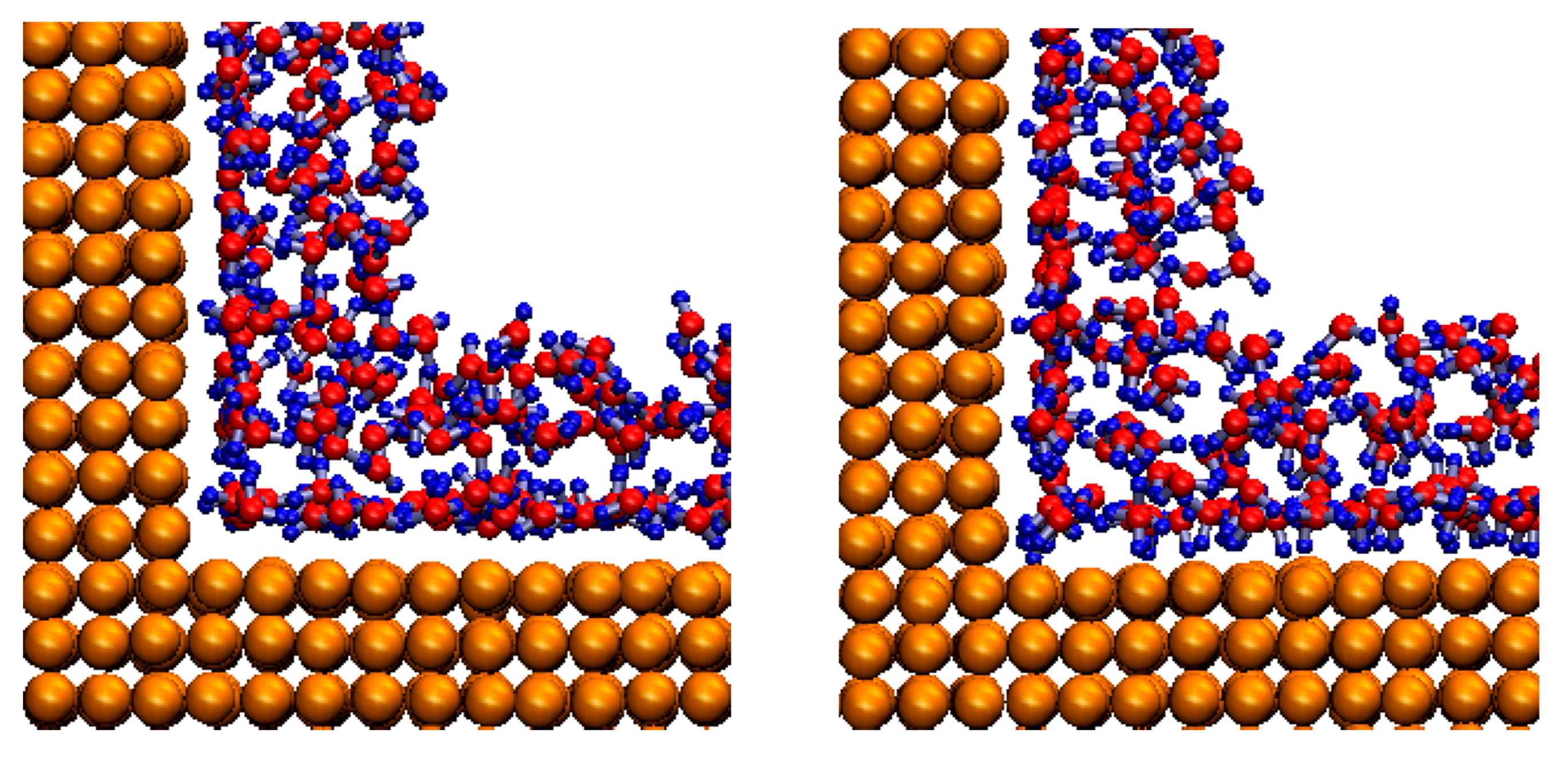
The overall resistance can be treated as a combination of the fluid and solid thermal resistances Rf and Rs (the solid wall separates two fluid reservoirs). Changes on the solid side due to the formation of sub-nanometer scale thermal boundary layers, which were our focus, had not previously been considered significant and had been attributed to the finite solid-side thermal conductivity [3,42]. Our results indicated that these interfacial resistances decreased the wall heat flux by order of magnitude when compared to a hypothetical system in which the overall fluid-solid contact resistances are negligible (as might occur at very large scales) [3]. In another investigation, we examined changes in the solid phase and studied the relationship between the surface properties and the nature of the fluids examined. Our studies showed that surface modifications of the type included could lead to over six-fold increase in heat transfer rates in a typical nano-devices. Interfaces near hydrophilic walls were found to be more structured with water near the walls. This observation was also confirmed by examining a snapshot of the molecules near the wall, as shown in Figure 4. From the snapshot on the right, it could be seen that the hydrogen atoms were pointing towards the hydrophilic wall, while, for hydrophobic walls, the left snapshot showed no such clear structure. Since hydrophilic walls attracted water molecules closer to the wall, thus, the first adsorption peak ended up closer to the wall. As a result, this increased the κ⊥ value significantly. These observations pointed to some exciting practical applications. If the outside wall of a house were to be made hydrophilic, during a hot summer day when it would be helpful to reduce heat transfer from the ambient (Ta > Tin), a polar fluid like water could be introduced between the two walls. At night, in order to cool the house (when Tin > Ta), water could be replaced by a less polar soft material to enhance heat transfer. Thus, the same wall would demonstrate significant rectification in different directions but with different fluids [43].
3.1.2. The Fluid-Fluid Interface
Fluid phases exhibit characteristics different from solids, so we examined how thermal transport could show rectification at the interface of immiscible water and hexane layers and investigated how that differs from solid-liquid interfaces. We found that depending on which fluid was on the hot- or cold-sides, the heat flux changed significantly (e.g., when either water or hexane was placed on the hot side). This clearly demonstrated that thermal rectification could be observed in liquid-liquid interfaces too. The magnitude of the rectification was influenced by the relative thicknesses of the layers. It was found to be highest when the water-hexane interface temperatures were equal for those two cases when either hexane was on the hot side or water on the hot side. The nature of the fluid (such as hexane), which has a lower thermal conductivity, had a bigger impact on the magnitude of the rectification than a fluid, such as water, with higher thermal conductivity. In addition, if interfacial temperature discontinuities could be introduced across macroscale interfaces as is natural for nanoscale systems, these would also lead to a significant increase in rectification [44].
Our investigations also indicated that liquid-liquid interfaces exhibited behavior significantly different than solid-fluid interfaces. We noted that the thermal resistance of a hexane-water interface was dependent on the interfacial temperature gradient alone, with only a small dependence on the average interfacial temperature; in contrast, that for the solid-liquid interface was significantly dependent on the interfacial temperature. Introducing a heat flux also resulted in a large increase in the liquid-liquid interface thickness compared to an equilibrium isothermal interface. Liquid-liquid interfaces have potential applications in a wide range of applications, e.g., sensors for wastewater treatment and removal of toxic ions from water; they could be designed to be more efficient by applying a heat flux. This might allow the interface to be used for applications not currently possible because of the very limited thickness of the interface in isothermal systems [45].
3.1.3. The Solid-Solid Interface
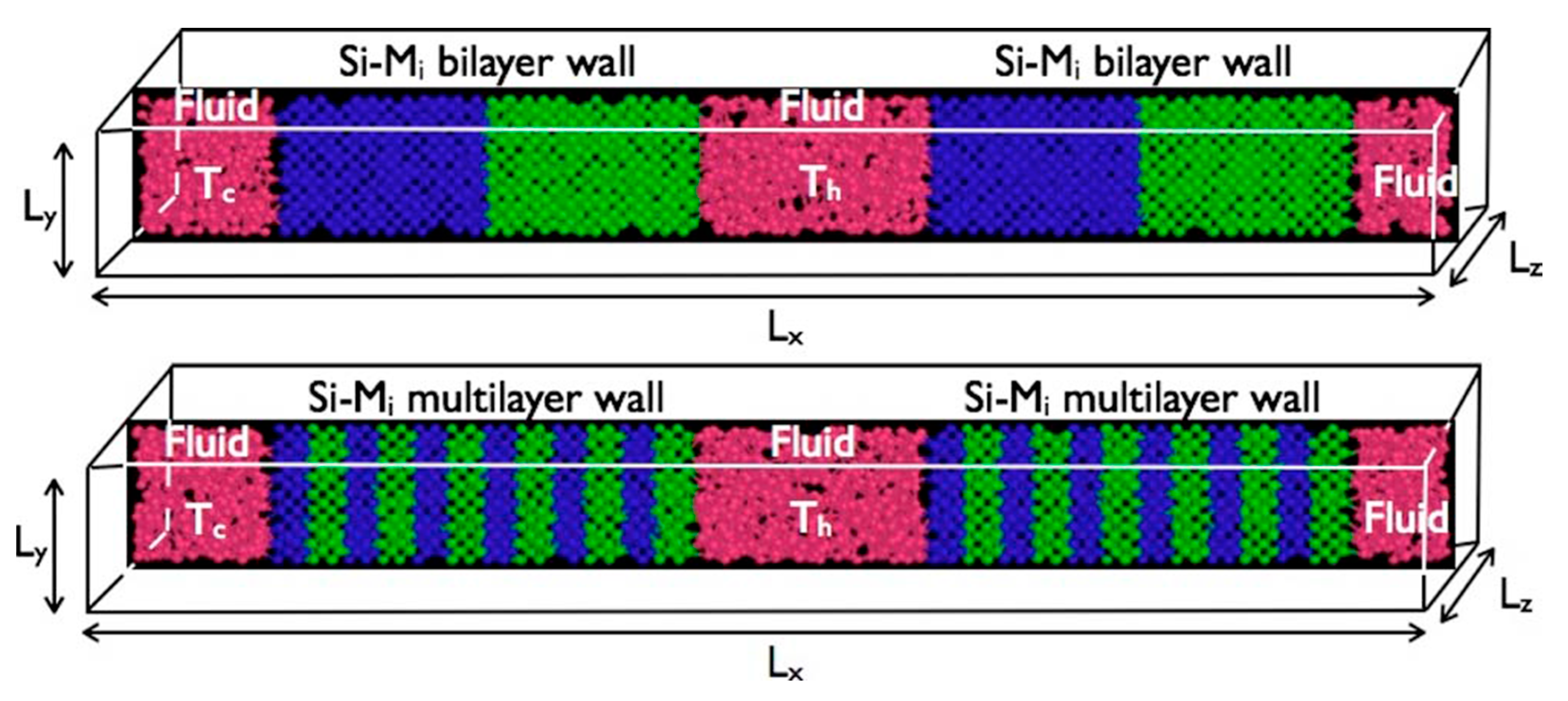
To investigate the system arrangements that would affect the thermal transport through superlattice solid-solid interfaces, we built composite walls with two or multiple layer solid films (with alternating layers of Si and an arbitrary molecule similar to Si but with a larger atomic diameter), shown in Figure 5. These superlattices were then placed between two hot and cold water-reservoirs at uniform temperatures. We found that increasing the number of composite Si–Mi layers in the solid walls led to a higher thermal resistance to heat transfer. For example, a six-bilayer Si–Mi wall conducted significantly less heat than a corresponding single bilayer composite wall of the same thickness [42]. We did not believe such a large reduction in thermal transport could be explained by the interfacial resistance alone. In addition, the relatively wide thermal boundary layers that were produced adjacent to the interfaces also introduced a supplementary resistance [46]. We speculated that this observation had significant implications for the design of semiconductor and related electronic devices that dissipate energy as heat. Thus, depending upon the desired outcome, it might be advantageous to either have composite films constructed in several alternating layers to inhibit heat transfer or else have fewer layers present if the thermal transport is to be enhanced [42].
3.2. The Anisotropy of Thermal Conductivity at Interfacial Layers
3.2.1. The Anisotropy for Solid-Liquid Interfaces
By using the system set-up shown in Figure 1 (with water as the fluid and copper as the solid wall), we were able to investigate thermal transport both parallel and perpendicular to the interface at the same time. We thermostated the hot and cold walls at different temperatures to test differential temperature effects on the anisotropy of thermal conductivity of the interfacial layers. The interfacial thermal resistance (R) was estimated using the Fourier equation (R = −∇T/q, noting that κ = 1/R). For the perpendicular interfacial resistance, we obtained the heat removed or added for the copper walls in the hatched yellow and blue areas and obtained the temperature gradient in the green interfacial region. For the parallel interfacial resistance, we once again obtained the heat added or removed in the hot (yellow unhatched) and cold (blue unhatched) walls in the region aligned with the red hatched interfacial regions, where we obtained the temperature gradient.
As explained in our recent previous publication, the anisotropy of thermal conductivity of the solid-liquid interface could be explained as follows: for heat transferred across (perpendicular to the) interfacial layer δ⊥, the phonons moving from the hot area to the cold area have to first across a region adjacent to the solid surface where the density is low, then across the first adsorption shell where the density is high, and again through another density trough [5]. The presence of density discontinuities reduces the heat transfer rate significantly. In contrast, in the parallel direction, while heat transfer along low-density regions is again diminished, overall thermal transport occurs far more effectively along stratified higher density layers. Since heat transfer occurs more effectively through δ|| than in the bulk fluid, nanoscale strategies should consider dissipating heat along such interfaces rather than through the bulk fluid. This can be seen from the density profiles shown in Figure 6.
Extending our previous study on anisotropy, we now examined the effect of temperature as well as temperature gradient on the observed anisotropy of the interfacial thermal resistance. We varied one of the two variables, average temperature (⟨T⟩) or temperature gradient (∇T), individually in two sets of simulations: In the first set, the hot/cold walls were maintained at 600/500 K, 550/450 K, 500/400 K, 450/350 K, and 400/300 K while keeping ∇T constant at 2.305 K/Å. In the second set, the average temperature was kept constant at 400 K with the hot/cold walls maintained at 525/275 K, 500/300 K, 475/325 K, 450/350 K, and 425/375 K, respectively, resulting in gradients from 1.153 to 5.673 K/Å. Finally, in the last set, we picked random points from the first and second sets to study systems in which both ⟨T⟩ and ∇T were varied simultaneously. We also studied both hydrophobic and hydrophilic walls, by either keeping the copper atoms uncharged or artificially adding a positive or negative charge of 0.1 e to alternating atoms in the wall. A summary of the results so obtained are shown in Table 1 for hydrophobic (uncharged) solid walls, and Table 2 for hydrophilic (charged) solid walls.
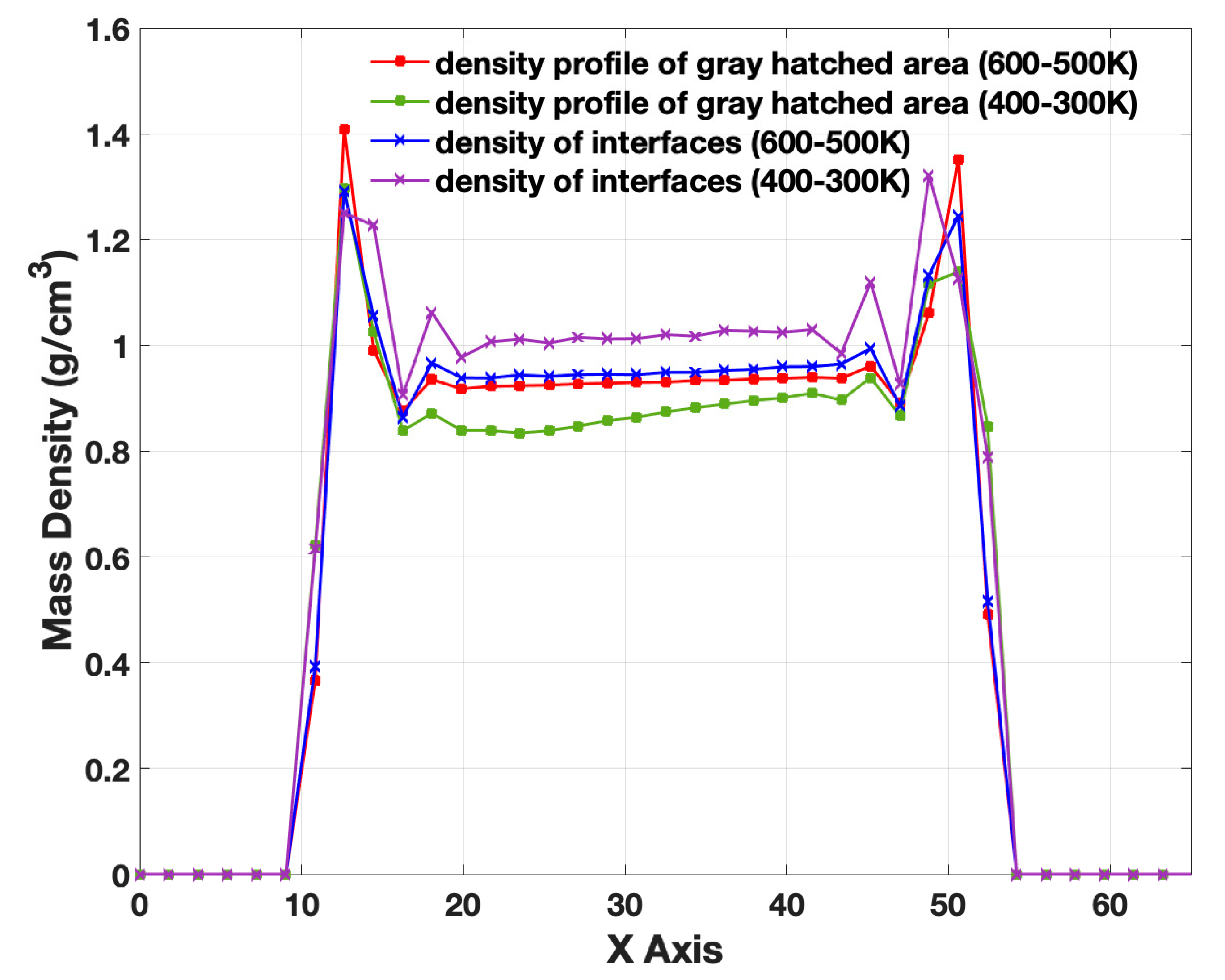
The results, shown in both Table 1 and Table 2, indicate that the anisotropy of thermal conductivity (κ||/κ⊥) decreased as the temperature was increased. This behavior could be explained by observing the density profiles for two different average temperatures (but constant temperature gradients) shown in Figure 6. The results showed that as the average temperature decreased, the density of the bulk phase decreased (cf. red and green lines) while the density of the interface concomitantly increased (blue and purple lines). Since anisotropy was strongly dependent on the density of the interface, this led to the higher anisotropy observed at the lower temperatures. The density of the interface (adsorption layer) was lower at higher temperatures because water molecules have more kinetic energy, which consequently hinders adsorption. The higher interfacial density, as indicated previously, had a much larger effect on the parallel thermal conductivity (κ||) compared to κ⊥, which led to the trends observed. Similar trends were observed in the density profiles for hydrophilic (charged) walls, and the simulation results for the anisotropy also showed similar behavior. The observed differences in the anisotropy of hydrophilic and hydrophobic walls have been discussed later in this section.
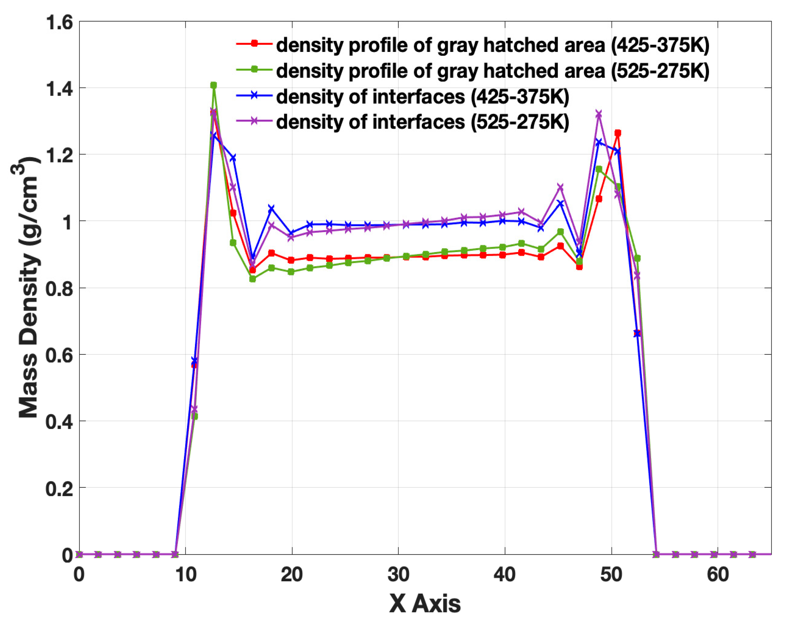
Figure 7 shows changes in density profiles when the average temperature is constant, but the temperature gradient varies. Although the average densities of interfacial layers were quite close (0.944 vs. 0.945 g/cm3), we could observe from Table 1 that the temperature gradient increased the anisotropy. This behavior in anisotropy could be explained by observations reported earlier [5]. The perpendicular thermal resistance (1/κ⊥) was significantly greater at lower temperatures than higher temperatures. With higher gradients (but equal average temperatures), the cold wall temperature was lower, which, as expected, resulted in lower values of κ⊥. While κ|| was also impacted by the higher gradient (the interfacial density, as seen in Figure 6, showed higher densities near the cold end and lower near the hot end), the change was primarily driven by the significantly decreasing value of κ⊥.
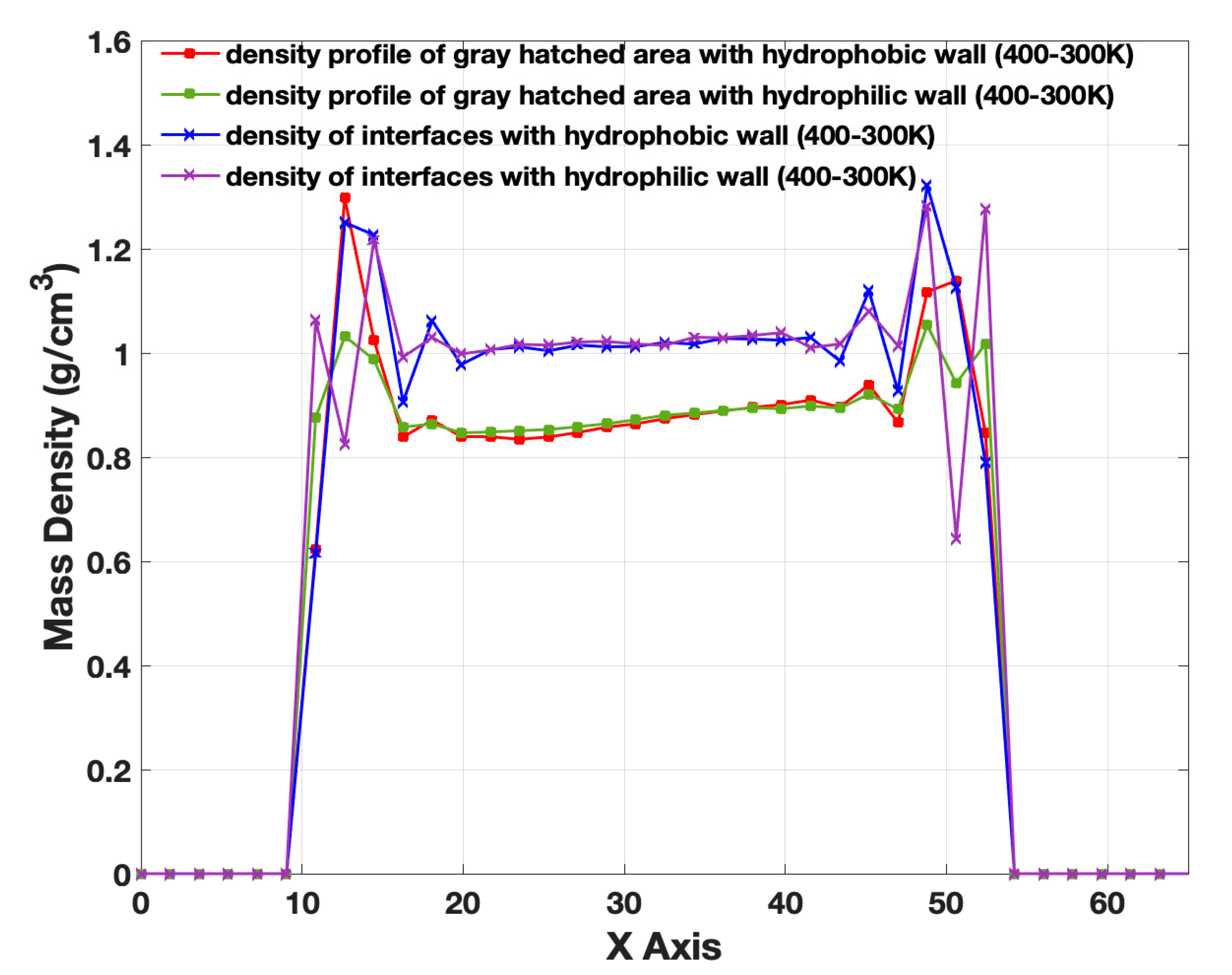
The results for hydrophobic walls are shown in Table 2. Figure 8 shows the density profiles for hydrophobic (uncharged) compared with hydrophilic walls. Results shown in Figure 8 are for equal temperatures (hot-cold: 400–300 K) for cases B5 and E5 in Table 2. The density profiles in Figure 8 show that when the wall was hydrophilic, the first adsorption shell was significantly closer to the wall. Furthermore, with hydrophilic walls, two adsorption peaks were observed, which indicated a more structured behavior of water near the walls. This behavior was also confirmed by a snapshot of the molecules near the wall, shown in Figure 4. The snapshot in Figure 4, right, showed that the hydrogen atoms were pointing towards the hydrophilic wall, while the left snapshot showed no obvious structure in the case of hydrophobic walls. A hydrophilic wall attracted water molecules closer to the wall; thus, the first adsorption peak was closer to the wall. This then increased the κ⊥ value significantly, which was confirmed in Figure 4 shown in the previous section. In addition, Figure 8 also shows that the density of the interface was essentially the same for both walls. This would indicate that κ|| would not change significantly and that the increase in κ⊥ would lead to the anisotropy being lower with hydrophilic walls.
The values reported in Table 1 and Table 2 showed results for five different temperatures while the gradients were constant (cases A1–A5; D1–D5), and five different temperature gradients while average temperatures were constant (cases B1–B5; E1 and E5). Within the expected accuracy of the simulations, the behavior observed was monotonic and could be interpolated. To investigate if the changes with respect to average temperatures and temperature gradients are correlated, we carried out five additional simulations where both the average temperatures were randomly changed for the cases previously studied. To investigate this, we first made ∇T dimensionless by reducing it by the melting temperature of water (273 K) divided by the system length in the x-direction (43.38 Å), resulting in a reducing parameter of 6.293 K/Å.
We then did a simple linear fit of the data for cases A1–A5, B1–B5, and D1–D5, E1–E5 separately using the equation
In Equation (1), the quantities a, b, c are three independent empirical parameters. For the hydrophobic wall, the resulting parameters were a = 1.977, b = −1.387, and c = 6.907, while for hydrophilic walls, a = 1.108, b = −0.980, and c = 4.601. We then used Equation (1) to predict values obtained in the simulations for cases C1–C5, F1–F5. Our results indicated that the predictions were well within the estimated accuracy of the simulated values. This indicated little or no correlation between the effect of the average temperature and the temperature gradient since we did not need to use a cross term in our empirical model.
3.2.2. The Anisotropy of Liquid-Liquid Interfaces
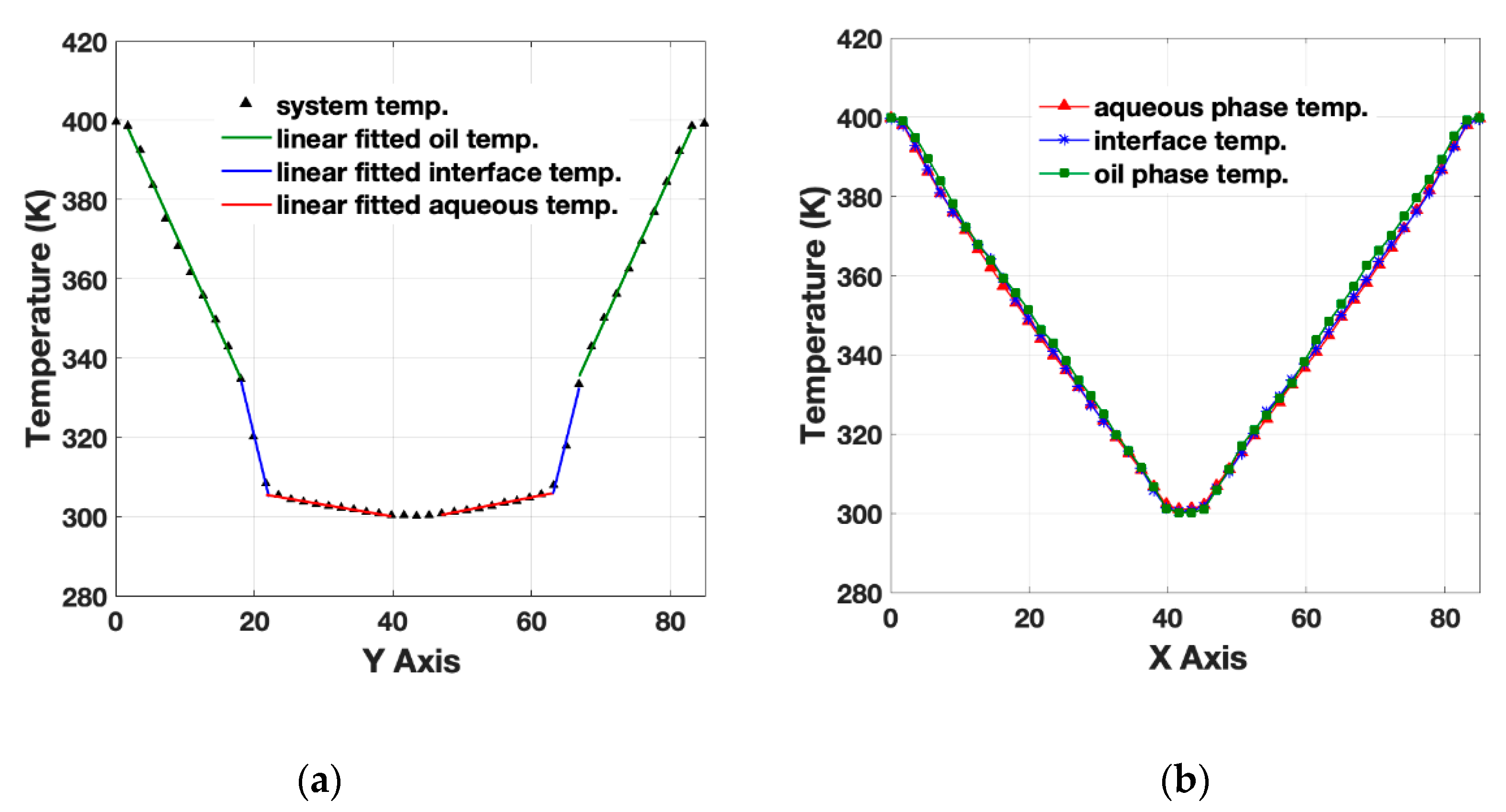
Figure 9 shows the temperature profiles of n-hexane (at 400 K) and water (at 300 K), corresponding to case 8 in Table 3. Figure 9a refers to the system of Figure 2a (for investigating the perpendicular interfacial thermal conductivity), while Figure 9b refers to the system of Figure 2b (for investigating the parallel interfacial thermal conductivity). The bulk phases and interfaces were identified with distinct colors consistent with those used in Figure 2a,b. The density profiles, shown in Figure 10 (corresponding to case 8 in Table 3), were also used to divide the system (see Figure 2) into the oil phase, the interface region, and the water phase. The interfaces include all the transition regions shown in Figure 10. According to Fourier’s equation, a larger temperature gradient (∇T) led to a smaller thermal conductivity with the same heat flux, which could be used to explain the discontinuity of ∇T in a different section in Figure 9. The ∇TH2O, shown in Figure 9a, was smaller in magnitude than ∇Thexane since water is a better thermal conductor than n-hexane. It is also obvious from the figure that the thermal conductivity of the interface was significantly smaller than those of both bulk aqueous and oil phases (∇Tint > ∇TH2O or ∇Thexane). This could be explained by the Kapitza effect between two immiscible liquids introduced by the discontinuity of materials. In Figure 9b, we have shown temperature profiles of water, oil, and interface, the side view in the y-z plane, using the system set-up shown in Figure 2b. Three profiles closely overlapped each other, which confirmed that there was no temperature gradient in the y-direction between the two phases, ensuring that the heat flux flows along the x-direction only and perpendicular to the y-z plane.
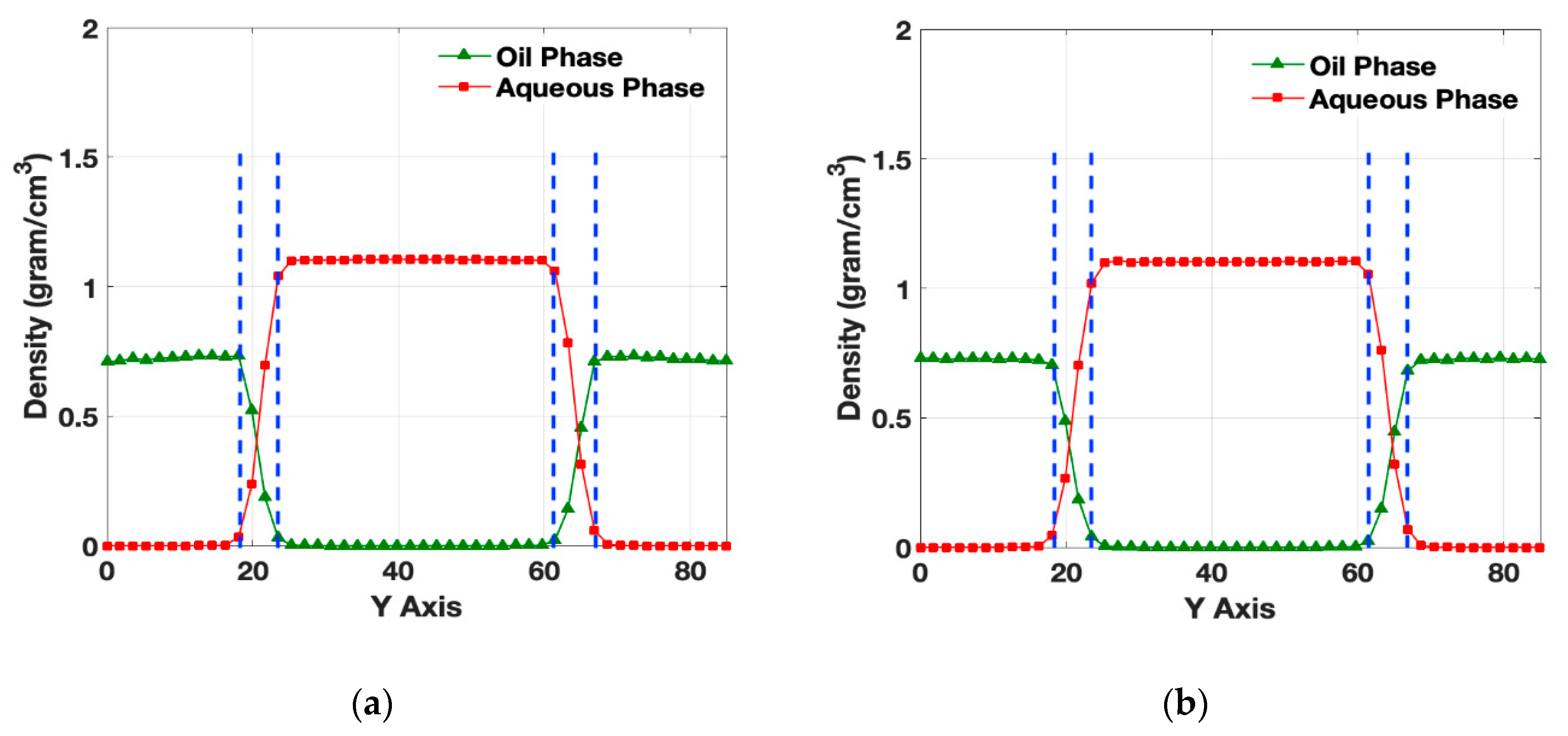
Figure 10a,b shows the density profiles of n-hexane and water (corresponding to case 8 in Table 3). Unlike the density discontinuity found between the solid and liquid regions previously, liquids being more mobile than solids, no such discontinuity was observed in the density profile in Figure 10. Another interesting observation was that, although the thermostatted regions were different in Figure 2a,b, the density profiles appeared to be strikingly similar. This was the case because our simulations were in the constant volume ensemble, so while the density profiles appeared similar, there would be significant differences in the pressure profiles of the two cases. Other systems studied gave qualitatively similar results to those reported in Figure 9 and Figure 10, so here we have provided only one case as an example.
Results from all the cases studied are summarized in Table 3. The ratios of κ||/κ⊥ were without exception greater than one, which indicated that heat was transferred more efficiently along the direction parallel to the interface, as was the case in the solid-liquid interface.
We believed the reason for this anisotropy in the liquid-liquid interface was similar to that for the liquid-solid interface. When the heat was transferred perpendicular to the interface, it had to overcome the liquid-liquid Kapitza effect resistance introduced by the liquid-liquid interface. But when it was parallel to the interface, it could be transferred along the two liquids and did not need to go across the interface between the liquids, bypassing the Kapitza effect at the liquid-liquid interface. The results also showed that the anisotropy depended on the nature of the liquid: solvents with larger molecules, like cyclohexane and linear hexane, exhibited stronger anisotropy than solvents with smaller molecules, like chloroform and carbon tetrachloride. This difference could be explained as follows: The perpendicular thermal conductivity (compared to the bulk oil thermal conductivity) for the oil phase in n-hexane drops significantly more than for the oil phase in carbon tetrachloride, for example. At the same time, the parallel thermal conductivity increases. This results in the higher anisotropy observed and reported in Table 3.
To emphasize the enhancement of thermal conductivity in the parallel direction in the interface shown in the last column of Table 3, we also compared the parallel value with its “effective value”, which are defined as [47];
where δint, δH2O, and δoil are, respectively, the thicknesses of the interface (defined as the thickness between the two vertical blue lines in Figure 10b), the water interface (defined as the distance between the endpoint of the bulk water density indicated by the vertical blue line and the point when the water and oil densities intersect), and the oil interfacial layer (defined similarly). In the column of κ||/κeff in Table 3, we observed that the values were all greater than 1, which means that Equation (2), used to estimate mixture thermal conductivity classically where thermal resistances are added in series, underestimates κ|| for interfaces at the microscopic level. This confirmed our conclusion that heat transfer took place more efficiently across the interface than even in the bulk fluid.
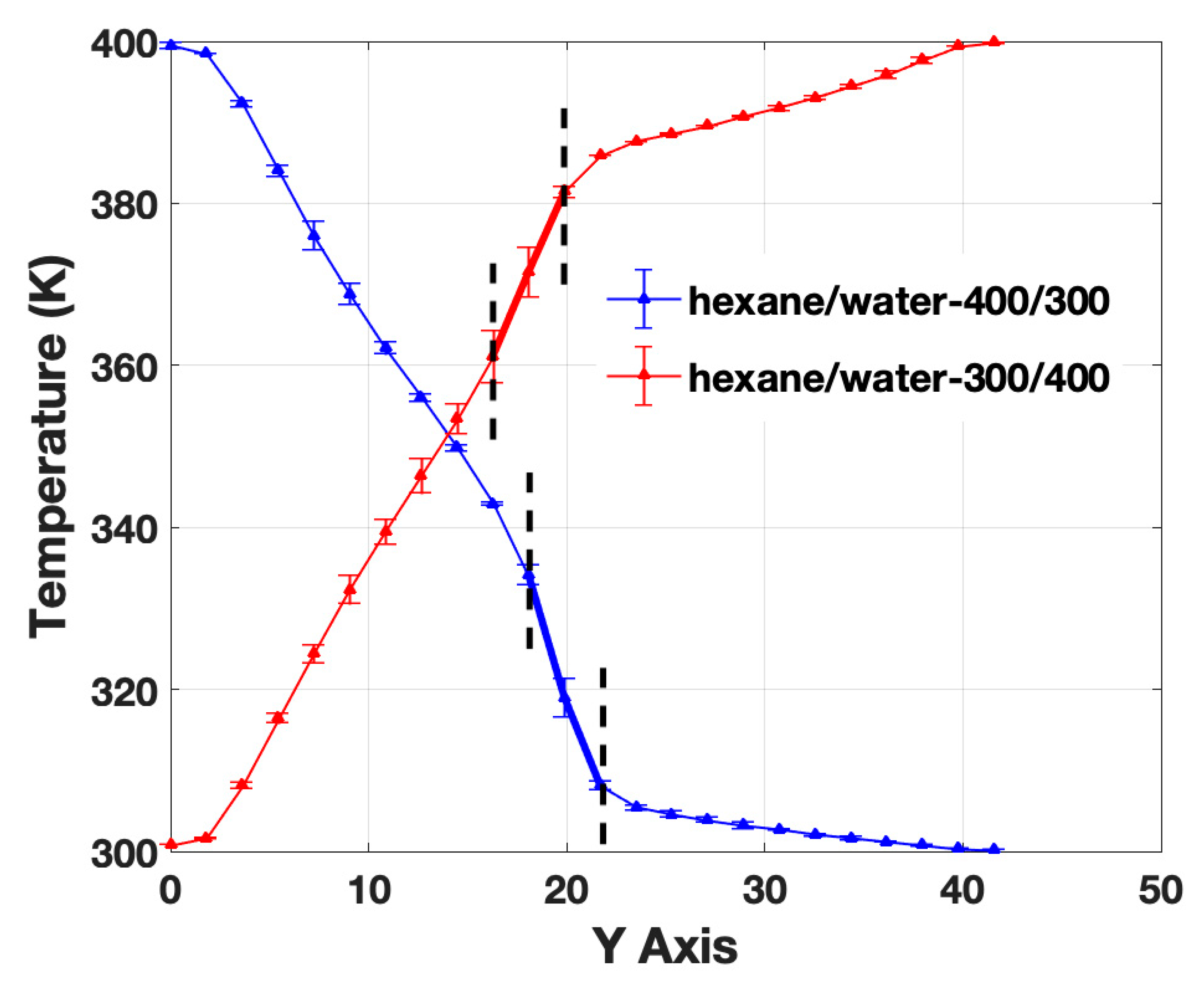
We also found that the system set-up was important when the heat flux was in the direction perpendicular to the interface (cases 2 and 3, likewise 7 and 8). In these two pairs of cases, if we were to swap the hot and cold thermostatted regions (keeping all other conditions the same), we observed, for example, from Figure 11 that ∇T of the interface region was more distinctive in case 8—water on the cold side (blue line: ∇Tint/∇Toil = 1.8) compared with case 7—hexane on the cold side (red line: ∇Tint/∇Toil = 1.3). In addition, the interface temperature of case 7 (red line) was higher than that of case 8 (blue line). Since higher temperatures (higher kinetic energy) increased molecular mobility, this resulted in increases in interfacial densities between two immiscible phases. Thus, a higher temperature led to higher interfacial thermal conductivity perpendicular to the interface. We observed that such a switch of the hot and cold phases led to a 10% change in heat transfer between cases 7 and 8. Similar results were observed for cases 2 and 3.
3.2.3. The Anisotropy of Solid-Solid Interfaces
In our study, we used two metal materials—silver and gold—to investigate the anisotropy of the interface. We carried out two simulations using the system set-up shown in Figure 3. The hot regions of both cases were maintained at 650 K, while the cold was at 450 K. We used a similar method as in the liquid-liquid study. The calculated anisotropy (κ||/κ⊥) was found to be 3.02 ± 0.05, which again confirmed our conclusion that heat transfer in the parallel direction led to higher heat transfer rates because it could effectively bypass the Kapitza effect in the solid-solid interface. This behavior appeared to be similar to that in solid-fluid and liquid-liquid interfaces.
4. Conclusions
The results presented in this paper showed that molecular dynamics is a useful and reliable tool to investigate interfacial thermal resistances. While such resistances are measurable, the experiments are rather expensive and time-consuming. Besides providing a molecular-level understanding of the physics underlying interfacial thermal resistance, the simulation studies also indicate several strategies that could be employed to increase the efficacy of heat dissipation in high power-consuming nano-devices over that in current designs. Since heat transfer occurs anisotropically, more effectively along the interfacial surface than in the bulk fluid, nanoscale strategies should consider dissipating heat along such interfaces rather than through the bulk fluid. Many of these strategies can be equally applicable to solid-liquid, liquid-liquid, and solid-solid interfaces.
Author Contributions
X.W. carried out the simulations, and all authors contributed to writing the manuscript. All authors have read and agreed to the published version of the manuscript.
Funding
This research was supported by grants from the National Science Foundation (CBET 1545560).
Conflicts of Interest
The authors declare no conflict of interest.
References
- Kapitza, P.L. Heat transfer and superfluidity of helium ii. Phys. Rev. 1941, 60, 354–355. [Google Scholar] [CrossRef]
- Murad, S.; Puri, I.K. Thermal transport across nanoscale solid-fluid interfaces. Appl. Phys. Lett. 2008, 92, 133105. [Google Scholar] [CrossRef] [Green Version]
- Murad, S.; Puri, I.K. Thermal transport through a fluid-solid interface. Chem. Phys. Lett. 2009, 476, 267–270. [Google Scholar] [CrossRef]
- Murad, S.; Puri, I.K. A thermal logic device based on fluid-solid interfaces. Appl. Phys. Lett. 2013, 102, 193109. [Google Scholar] [CrossRef] [Green Version]
- Wang, X.; Venerus, D.; Puri, I.K.; Murad, S. On using the anisotropy in the thermal resistance of solid-fluid interfaces to more effectively cool nano-electronics. Mol. Simul. 2019, 46, 162–167. [Google Scholar] [CrossRef]
- Suleiman, B.M.; Larfeldt, J.; Leckner, B.; Gustavsson, M. Thermal conductivity and diffusivity of wood. Wood Sci. Technol. 1999, 33, 465–473. [Google Scholar] [CrossRef]
- Xu, Y.; Chen, X.; Gu, B.-L.; Duan, W. Intrinsic anisotropy of thermal conductance in graphene nanoribbons. Appl. Phys. Lett. 2009, 95, 233116. [Google Scholar] [CrossRef] [Green Version]
- Roh, J.W.; Hippalgaonkar, K.; Ham, J.H.; Chen, R.; Li, M.Z.; Ercius, P.; Majumdar, A.; Kim, W.; Lee, W. Observation of anisotropy in thermal conductivity of individual single-crystalline bismuth nanowires. ACS Nano 2011, 5, 3954–3960. [Google Scholar] [CrossRef]
- Hennig, J.; Knappe, W. Anisotropy of thermal conductivity in stretched amorphous linear polymers and in strained elastomers. J. Polym. Sci. Part C Polym. Symp. 1964, 6, 167–174. [Google Scholar] [CrossRef]
- Renteria, J.D.; Ramirez, S.; Malekpour, H.; Alonso, B.; Centeno, A.; Zurutuza, A.; Cocemasov, A.I.; Nika, D.L.; Balandin, A.A. Strongly anisotropic thermal conductivity of free-standing reduced graphene oxide films annealed at high temperature. Adv. Funct. Mater. 2015, 25, 4664–4672. [Google Scholar] [CrossRef]
- Luo, Z.; Maassen, J.; Deng, Y.; Du, Y.; Garrelts, R.P.; Lundstrom, M.S.; Ye, P.D.; Xu, X. Anisotropic in-plane thermal conductivity observed in few-layer black phosphorus. Nat. Commun. 2015, 6, 8572. [Google Scholar] [CrossRef] [PubMed]
- Graebner, J.E.; Jin, S.; Kammlott, G.W.; Herb, J.A.; Gardinier, C.F. Large anisotropic thermal conductivity in synthetic diamond films. Nature 1992, 359, 401–403. [Google Scholar] [CrossRef]
- Crommie, M.F.; Zettl, A. Thermal-conductivity anisotropy of single-crystal Bi2Sr2CaCu2O8. Phys. Rev. B 1991, 43, 408–412. [Google Scholar] [CrossRef] [PubMed]
- Venkatasubramanian, R. Lattice thermal conductivity reduction and phonon localizationlike behavior in superlattice structures. Phys. Rev. B 2000, 61, 3091–3097. [Google Scholar] [CrossRef]
- Rondelez, F.; Urbach, W.; Hervet, H. Origin of thermal conductivity anisotropy in liquid crystalline phases. Phys. Rev. Lett. 1978, 41, 1058–1062. [Google Scholar] [CrossRef]
- Harada, M.; Ochi, M.; Tobita, M.; Kimura, T.; Ishigaki, T.; Shimoyama, N.; Aoki, H. Thermal-conductivity properties of liquid-crystalline epoxy resin cured under a magnetic field. J. Polym. Sci. Part B Polym. Phys. 2003, 41, 1739–1743. [Google Scholar] [CrossRef]
- Miller, M.G.; Keith, J.M.; King, J.A.; Edwards, B.J.; Klinkenberg, N.; Schiraldi, D.A. Measuring thermal conductivities of anisotropic synthetic graphite–liquid crystal polymer composites. Polym. Compos. 2006, 27, 388–394. [Google Scholar] [CrossRef]
- Wang, X.; Gu, X.; Murad, S. Molecular dynamics simulations of liquid-liquid phase equilibrium of ternary methanol/water/hydrocarbon mixtures. Fluid Phase Equilib. 2018, 470, 109–119. [Google Scholar] [CrossRef]
- Wang, R.H.; Knudsen, J.G. Thermal conductivity of liquid-liquid emulsions. Ind. Eng. Chem. 1958, 50, 1667–1670. [Google Scholar] [CrossRef]
- Zhao, B.; Oroskar, P.A.; Wang, X.; House, D.; Oroskar, A.; Oroskar, A.; Jameson, C.; Murad, S. The composition of the mobile phase affects the dynamic chiral recognition of drug molecules by the chiral stationary phase. Langmuir 2017, 33, 11246–11256. [Google Scholar] [CrossRef]
- Wang, X.; House, D.; Oroskar, P.; Oroskar, A.; Oroskar, A.; Jameson, C.; Murad, S. Molecular dynamics simulations of the chiral recognition mechanism for a polysaccharide chiral stationary phase in enantiomeric chromatographic separations. Mol. Phys. 2019, 117, 3569–3588. [Google Scholar] [CrossRef]
- Sofos, F.; Karakasidis, T.; Liakopoulos, A. Transport properties of liquid argon in krypton nanochannels: Anisotropy and non-homogeneity introduced by the solid walls. Int. J. Heat Mass Transf. 2009, 52, 735–743. [Google Scholar] [CrossRef]
- Liu, Y.; Wang, Q. Transport behavior of water confined in carbon nanotubes. Phys. Rev. B 2005, 72. [Google Scholar] [CrossRef]
- Ikeshoji, T.; Hafskjold, B. Non-equilibrium molecular dynamics calculation of heat conduction in liquid and through liquid-gas interface. Mol. Phys. 1994, 81, 251–261. [Google Scholar] [CrossRef]
- Müller-Plathe, F. A simple nonequilibrium molecular dynamics method for calculating the thermal conductivity. J. Chem. Phys. 1997, 106, 6082–6085. [Google Scholar] [CrossRef]
- Green, M.S. Markoff random processes and the statistical mechanics of time-dependent phenomena. Ii. Irreversible processes in fluids. J. Chem. Phys. 1954, 22, 398–413. [Google Scholar] [CrossRef]
- Kubo, R. Statistical-mechanical theory of irreversible processes. I. General theory and simple applications to magnetic and conduction problems. J. Phys. Soc. Jpn. 1957, 12, 570–586. [Google Scholar] [CrossRef]
- Qu, F.; Shi, R.; Peng, L.; Zhang, Y.; Gu, X.; Wang, X.; Murad, S. Understanding the effect of zeolite crystal expansion/contraction on separation performance of naa zeolite membrane: A combined experimental and molecular simulation study. J. Membr. Sci. 2017, 539, 14–23. [Google Scholar] [CrossRef]
- Chen, C.; Cheng, Y.; Peng, L.; Zhang, C.; Wu, Z.; Gu, X.; Wang, X.; Murad, S. Fabrication and stability exploration of hollow fiber mordenite zeolite membranes for isopropanol/water mixture separation. Microporous Mesoporous Mater. 2019, 274, 347–355. [Google Scholar] [CrossRef]
- Hinkle, K.; Wang, X.; Gu, X.; Jameson, C.; Murad, S. Computational molecular modeling of transport processes in nanoporous membranes. Processes 2018, 6, 124. [Google Scholar] [CrossRef] [Green Version]
- Wang, X.; Zhang, Y.; Wang, X.; Andres-Garcia, E.; Du, P.; Giordano, L.; Wang, L.; Hong, Z.; Gu, X.; Murad, S.; et al. Xenon recovery by dd3r zeolite membranes: Application in anaesthetics. Angew. Chem. Int. Ed. 2019, 58, 15518–15525. [Google Scholar] [CrossRef] [PubMed]
- Jorgensen, W.L.; Chandrasekhar, J.; Madura, J.D.; Impey, R.W.; Klein, M.L. Comparison of simple potential functions for simulating liquid water. J. Chem. Phys. 1983, 79, 926–935. [Google Scholar] [CrossRef]
- Foiles, S.; Baskes, M.; Daw, M.S. Embedded-atom-method functions for the fcc metals Cu, Ag, Au, Ni, Pd, Pt, and their alloys. Phys. Rev. B 1986, 33, 7983. [Google Scholar] [CrossRef] [PubMed]
- Jorgensen, W.L.; Madura, J.D.; Swenson, C.J. Optimized intermolecular potential functions for liquid hydrocarbons. J. Am. Chem. Soc. 1984, 106, 6638–6646. [Google Scholar] [CrossRef]
- Jorgensen, W.L. Optimized intermolecular potential functions for liquid alcohols. J. Phys. Chem. 1986, 90, 1276–1284. [Google Scholar] [CrossRef]
- Heinz, H.; Vaia, R.; Farmer, B.; Naik, R. Accurate simulation of surfaces and interfaces of face-centered cubic metals using 12–6 and 9–6 lennard-jones potentials. J. Phys. Chem. C 2008, 112, 17281–17290. [Google Scholar] [CrossRef]
- Hockney, R.W.; Eastwood, J.W. Computer Simulation Using Particles; Taylor & Francis Inc: Bristol, PA, USA, 1988. [Google Scholar]
- Martínez, L.; Andrade, R.; Birgin, E.G.; Martínez, J.M. Packmol: A package for building initial configurations for molecular dynamics simulations. J. Comput. Chem. 2009, 30, 2157–2164. [Google Scholar] [CrossRef]
- Plimpton, S. Fast parallel algorithms for short-range molecular dynamics. J. Comput. Phys. 1995, 117, 1–19. [Google Scholar] [CrossRef] [Green Version]
- Schneider, T.; Stoll, E. Molecular-dynamics study of a three-dimensional one-component model for distortive phase transitions. Phys. Rev. B 1978, 17, 1302. [Google Scholar] [CrossRef]
- Murad, S.; Puri, I.K. Communication: Thermal rectification in liquids by manipulating the solid-liquid interface. J. Chem. Phys. 2012, 137. [Google Scholar] [CrossRef]
- Murad, S.; Puri, I.K. Molecular simulations of thermal transport across interfaces: Solid-vapour and solid-solid. Mol. Simul. 2012, 38, 642–652. [Google Scholar] [CrossRef]
- Murad, S.; Puri, I.K. Dynamic rectification in a thermal diode based on fluid-solid interfaces: Contrasting behavior of soft materials and fluids. Appl. Phys. Lett. 2014, 104, 211601. [Google Scholar] [CrossRef]
- Murad, S.; Puri, I.K. Achieving thermal rectification in designed liquid-liquid systems. Appl. Phys. Lett. 2016, 108, 134101. [Google Scholar] [CrossRef] [Green Version]
- Murad, S.; Puri, I.K. Understanding the liquid–Liquid (water-hexane) interface. Chem. Phys. Lett. 2017, 685, 422–426. [Google Scholar] [CrossRef]
- Murad, S.; Puri, I.K. Thermal transport through superlattice solid-solid interfaces. Appl. Phys. Lett. 2009, 95, 051907. [Google Scholar] [CrossRef] [Green Version]
- Hasselman, D.P.H.; Johnson, L.F. Effective thermal conductivity of composites with interfacial thermal barrier resistance. J. Compos. Mater. 1987, 21, 508–515. [Google Scholar] [CrossRef]
Figure 1.
A Schematic (not to scale) of the 130.14 × 65.07 × 28.92 Å simulation system containing liquid confined within solid walls to be investigated. The yellow region indicates the hot copper wall (at temperature Th) Λh; in blue is the cold copper wall Λc (temperature Tc); in unhatched gray Λa, are copper wall sections where the temperature is not controlled (copper walls of 10.845 Å, 21.69 Å, and 10.845 Å thicknesses.) The Λh walls are at a higher temperature than Λc, resulting in heat transfer in the direction indicated (perpendicular to the green interface δ⊥ but parallel to the red interface δ|| that lies along the Λa). The gray hatched regions identify the “bulk” fluid (region away from the interfaces). The white regions at the intersection of the copper walls indicate “double” interfaces. These regions, because of this added complexity, are not used in our interfacial thermal resistance calculations. Reproduced with permission from [5], Copyright Taylor & Francis, 2019.

Figure 2.
Schematic of systems composed of three phases to study the liquid-liquid interfacial thermal conductivity. The simulation box dimensions are 86.76 × 86.76 × 28.92 Å. Different areas are self-explained in the figure. System (a) is used to study the interface when the heat is transferred along the direction perpendicular to the interface. The interfaces are denoted as δ⊥ in the text. System (b) is the parallel case, and the interfaces are denoted as δ||.

Figure 3.
Schematic of systems designed to study the solid-solid interfacial thermal conductivity. The simulation box dimensions are 49.08 × 98.16 × 49.08 Å. System (a) is designed for studies of the interfacial thermal conductivity parallel to the interface. This interface is referred to as δ|| in the text. System (b) is the design for the interfacial thermal conductivity perpendicular to the interface. The thickness of this interface is referred to as δ⊥.

Figure 4.
Snapshot of molecules close to the wall (only showing water molecules that are within 8 Å of copper wall atoms). Orange: copper atoms; red: oxygen atoms; blue: hydrogen atoms. Left: neutral wall; right: charged wall.
Figure 4.
Snapshot of molecules close to the wall (only showing water molecules that are within 8 Å of copper wall atoms). Orange: copper atoms; red: oxygen atoms; blue: hydrogen atoms. Left: neutral wall; right: charged wall.

Figure 5.
Schematic diagram of a domain based on an arbitrary simulation for systems with bilayer and six-layer composite Si (or M1) -Mi superlattice walls. Periodic boundary conditions apply on all six faces of the basic cyclically replicated parallelepiped. The domain dimensions are Lx = 20.99 nm and Ly = Lz = 2.172 nm. Reproduced with permission from [46], Copyright AIP Publishing, 2019.

Figure 6.
Mass density profile of water along the X (see Figure 1) direction when the average temperature is only varied—cases B1 and B5 (see Table 1 for conditions). The red and green lines represent the regions shown as the bulk phase (grey hatched areas) and the adjoining interface regions (green hatched areas) shown in Figure 1. The blue and purple lines, respectively, show the interface regions (red hatched areas) and the adjoining “double” interface regions (unhatched white) shown in Figure 1.

Figure 7.
Mass density profiles of water along the X direction when only the temperature gradient is varied (see Figure 1) for cases A1 and A5 (see Table 1 for conditions). The red and green lines represent the regions shown as the bulk phase (grey hatched areas) and the adjoining interface regions (green hatched areas) shown in Figure 1. The blue and purple lines, respectively, show the interface regions (red hatched areas) and the adjoining “double” interface regions (unhatched white) shown in Figure 1.

Figure 8.
Mass density profiles of water along the X-axis (Figure 1) when the copper wall is hydrophobic or hydrophilic, corresponding to cases B5 and E5 in Table 1 and Table 2. The red and green lines represent the regions shown as the bulk phase (grey hatched areas) and the adjoining interface regions (green hatched areas) shown in Figure 1. The blue and purple lines, respectively, show the interface regions (red hatched areas) and the adjoining “double” interface regions (unhatched white) shown in Figure 1.

Figure 9.
Temperature profiles of the n-hexane and water system, corresponding to case 8 at Table 3: (a) along the Y direction when the heat is transferred perpendicular to the interfaces shown in Figure 2a, (b) along the X direction when the heat is transferred parallel to the interfaces as shown in Figure 2b.

Figure 10.
Density profiles of n-hexane and water system. Blue vertical lines indicate the location of the interfaces. In case (a), heat is being transferred perpendicular to the interfaces, while, in case (b), heat is transferred parallel to the interfaces.
Figure 10.
Density profiles of n-hexane and water system. Blue vertical lines indicate the location of the interfaces. In case (a), heat is being transferred perpendicular to the interfaces, while, in case (b), heat is transferred parallel to the interfaces.

Figure 11.
Temperature profiles of the case 7 (red) and case 8 (blue) in Table 3. Profiles are averaged, and only half is shown here because of the symmetry of system setups. Error bars are calculated when folding the data. Vertical lines cut out the interfaces, and they are plotted using thicker lines.


Table 1.
Results for water with “hydrophobic” hot and cold copper walls maintained at the temperatures shown. Errors reported were estimated by changing the initial conditions.
Table 1.
Results for water with “hydrophobic” hot and cold copper walls maintained at the temperatures shown. Errors reported were estimated by changing the initial conditions.
| Series ID | Temperature Range (K) | ∇T (K/Å) | ∇T* | ⟨T⟩ (K) | ⟨T⟩* | κ||/κ⊥ | Predicted κ||/κ⊥ | Error (%) |
|---|---|---|---|---|---|---|---|---|
| A1 | 525–275 | 5.763 | 0.916 | 400 | 1.465 | 6.308 | 6.685 | 5.97 |
| A2 | 500–300 | 4.610 | 0.733 | 400 | 1.465 | 5.999 | 6.323 | 5.39 |
| A3 | 475–325 | 3.458 | 0.549 | 400 | 1.465 | 5.737 | 5.960 | 3.89 |
| A4 | 450–350 | 2.305 | 0.366 | 400 | 1.465 | 5.736 | 5.598 | 2.40 |
| A5 | 425–375 | 1.153 | 0.183 | 400 | 1.465 | 4.629 | 5.236 | 13.12 |
| B1 | 600–500 | 2.305 | 0.366 | 550 | 2.015 | 5.120 | 4.836 | 5.55 |
| B2 | 550–450 | 2.305 | 0.366 | 500 | 1.832 | 5.383 | 5.090 | 5.44 |
| B3 | 500–400 | 2.305 | 0.366 | 450 | 1.649 | 5.661 | 5.344 | 5.60 |
| B4 | 450–350 | 2.305 | 0.366 | 400 | 1.465 | 5.736 | 5.598 | 2.40 |
| B5 | 400–300 | 2.305 | 0.366 | 350 | 1.282 | 6.214 | 5.852 | 5.82 |
| C1 | 475–425 | 1.152 | 0.183 | 450 | 1.648 | 5.604 | 4.982 | 11.09 |
| C2 | 550–300 | 5.763 | 0.916 | 425 | 1.557 | 6.049 | 6.558 | 8.407 |
| C3 | 500–300 | 4.610 | 0.732 | 400 | 1.465 | 5.999 | 6.323 | 5.39 |
| C4 | 450–300 | 3.458 | 0.549 | 375 | 1.374 | 6.001 | 6.087 | 1.44 |
| C5 | 400–300 | 2.305 | 0.366 | 350 | 1.282 | 6.214 | 5.852 | 5.82 |
∇T, temperature gradient; ⟨T⟩, average temperature; κ, thermal conductivity.
Table 2.
Results for water confined by “hydrophilic” (artificially charged copper) walls for a range of temperatures and temperature gradients.
Table 2.
Results for water confined by “hydrophilic” (artificially charged copper) walls for a range of temperatures and temperature gradients.
| Series ID | Temperature Range (K) | ∇T (K/Å) | ∇T* | ⟨T⟩ (K) | ⟨T⟩* | κ||/κ⊥ | Predicted κ||/κ⊥ | Error (%) |
|---|---|---|---|---|---|---|---|---|
| D1 | 525–275 | 5.763 | 0.916 | 400 | 1.465 | 3.822 | 4.180 | 9.36 |
| D2 | 500–300 | 4.610 | 0.733 | 400 | 1.465 | 3.828 | 3.977 | 3.88 |
| D3 | 475–325 | 3.458 | 0.549 | 400 | 1.465 | 3.711 | 3.774 | 1.70 |
| D4 | 450–350 | 2.305 | 0.366 | 400 | 1.465 | 3.655 | 3.571 | 2.30 |
| D5 | 425–375 | 1.153 | 0.183 | 400 | 1.465 | 2.894 | 3.368 | 16.39 |
| E1 | 600–500 | 2.305 | 0.366 | 550 | 2.015 | 3.283 | 3.032 | 7.63 |
| E2 | 550–450 | 2.305 | 0.366 | 500 | 1.832 | 3.434 | 3.212 | 6.462 |
| E3 | 500–400 | 2.305 | 0.366 | 450 | 1.649 | 3.476 | 3.392 | 2.43 |
| E4 | 450–350 | 2.305 | 0.366 | 400 | 1.465 | 3.655 | 3.571 | 2.30 |
| E5 | 400–300 | 2.305 | 0.366 | 350 | 1.282 | 4.070 | 3.751 | 7.85 |
| F1 | 475–425 | 1.152 | 0.183 | 450 | 1.648 | 2.807 | 3.189 | 13.60 |
| F2 | 550–300 | 5.763 | 0.916 | 425 | 1.557 | 3.759 | 4.090 | 8.81 |
| F3 | 500–300 | 4.610 | 0.732 | 400 | 1.465 | 3.828 | 3.977 | 3.90 |
| F4 | 450–300 | 3.458 | 0.549 | 375 | 1.374 | 3.836 | 3.836 | 0.72 |
| F5 | 400–300 | 2.305 | 0.366 | 350 | 1.282 | 4.070 | 3.751 | 7.85 |
Table 3.
Ratios of the parallel interfacial thermal conductivities κ|| over perpendicular conductivities κ⊥, water thermal conductivities κH2O, the oil thermal conductivities κoil, and effective thermal conductivities κeff.
Table 3.
Ratios of the parallel interfacial thermal conductivities κ|| over perpendicular conductivities κ⊥, water thermal conductivities κH2O, the oil thermal conductivities κoil, and effective thermal conductivities κeff.
| Case | System (Cold/Hot) | Temperature Range | κ||/κ⊥ | κ|| a/κH2O b | κ|| a/κoil b | κ|| a/κeff c |
|---|---|---|---|---|---|---|
| 1 | CHCl3/H2O | 275–325 K | 1.77 ± 0.53 | 0.52 ± 0.02 | 4.21 ± 0.78 | 2.63 ± 0.28 |
| 2 | CHCl3/H2O | 300–400 K | 4.43 ± 0.41 | 0.51 ± 0.02 | 3.97 ± 0.54 | 2.24 ± 0.22 |
| 3 | H2O/CHCl3 | 300–400 K | 5.96 ± 0.20 | 0.51 ± 0.02 | 3.97 ± 0.54 | 2.24 ± 0.22 |
| 4 | CCl4/H2O | 295–345 K | 2.73 ± 0.66 | 0.53 ± 0.08 | 4.38 ± 1.25 | 2.73 ± 0.08 |
| 5 | Cyclohexane/H2O | 300–350 K | 8.17 ± 0.96 | 0.64 ± 0.05 | 5.90 ± 1.90 | 3.64 ± 0.72 |
| 6 | n-Hexane/H2O | 275–325 K | 6.08 ± 1.03 | 0.57 ± 0.07 | 5.41 ± 0.96 | 3.34 ± 0.10 |
| 7 | n-Hexane/H2O | 300–400 K | 5.53 ± 1.02 | 0.52 ± 0.06 | 4.15 ± 0.86 | 2.34 ± 0.07 |
| 8 | H2O/n-Hexane | 300–400 K | 7.79 ± 1.11 | 0.52 ± 0.06 | 4.15 ± 0.86 | 2.34 ± 0.07 |
a Ratios of κ⊥ can be calculated from κ||/κ⊥ and other columns. b κH2O and κoil are calculated from aqueous and oil phases shown in Figure 2b. c κeff is calculated through Equation (2).
© 2019 by the authors. Licensee MDPI, Basel, Switzerland. This article is an open access article distributed under the terms and conditions of the Creative Commons Attribution (CC BY) license (http://creativecommons.org/licenses/by/4.0/).
Share and Cite
MDPI and ACS Style
Wang, X.; Jameson, C.J.; Murad, S. Interfacial Thermal Conductivity and Its Anisotropy. Processes 2020, 8, 27. https://doi.org/10.3390/pr8010027
AMA Style
Wang X, Jameson CJ, Murad S. Interfacial Thermal Conductivity and Its Anisotropy. Processes. 2020; 8(1):27. https://doi.org/10.3390/pr8010027
Chicago/Turabian StyleWang, Xiaoyu, Cynthia J. Jameson, and Sohail Murad. 2020. "Interfacial Thermal Conductivity and Its Anisotropy" Processes 8, no. 1: 27. https://doi.org/10.3390/pr8010027
Note that from the first issue of 2016, this journal uses article numbers instead of page numbers. See further details here.