
Exploring Partial Structural Disorder in Anhydrous Paraxanthine through Combined Experiment, Solid-State Computational Modelling, and Molecular Docking


Abstract
:
1. Introduction
2. Materials and Methods
2.1. Material
2.2. Methods
Experimental Nuclear Quadrupole Resonance (NQR)
2.3. Computational Density Functional Theory
2.3.1. Spectra Simulation—Cluster Technique
2.3.2. Spectra Simulation—Solid-State Technique
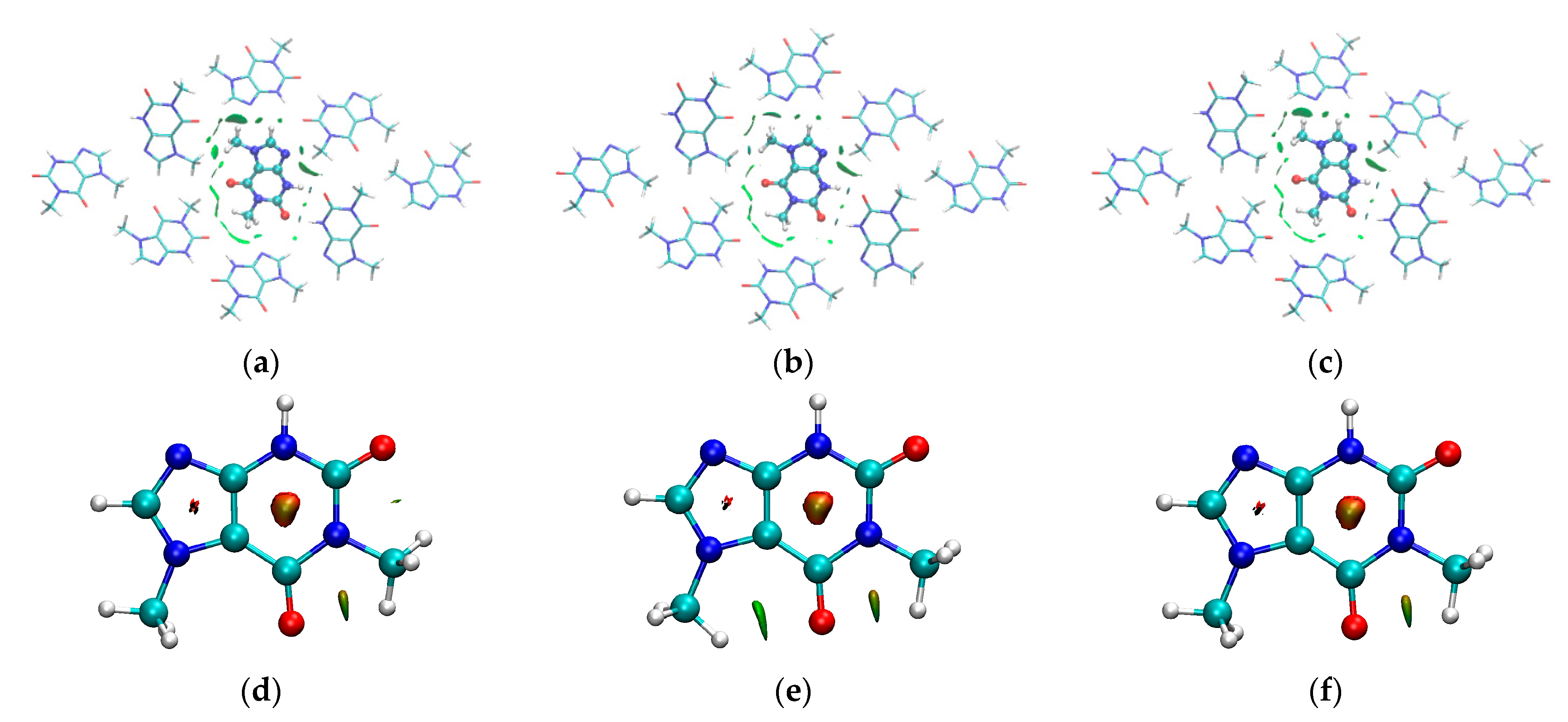
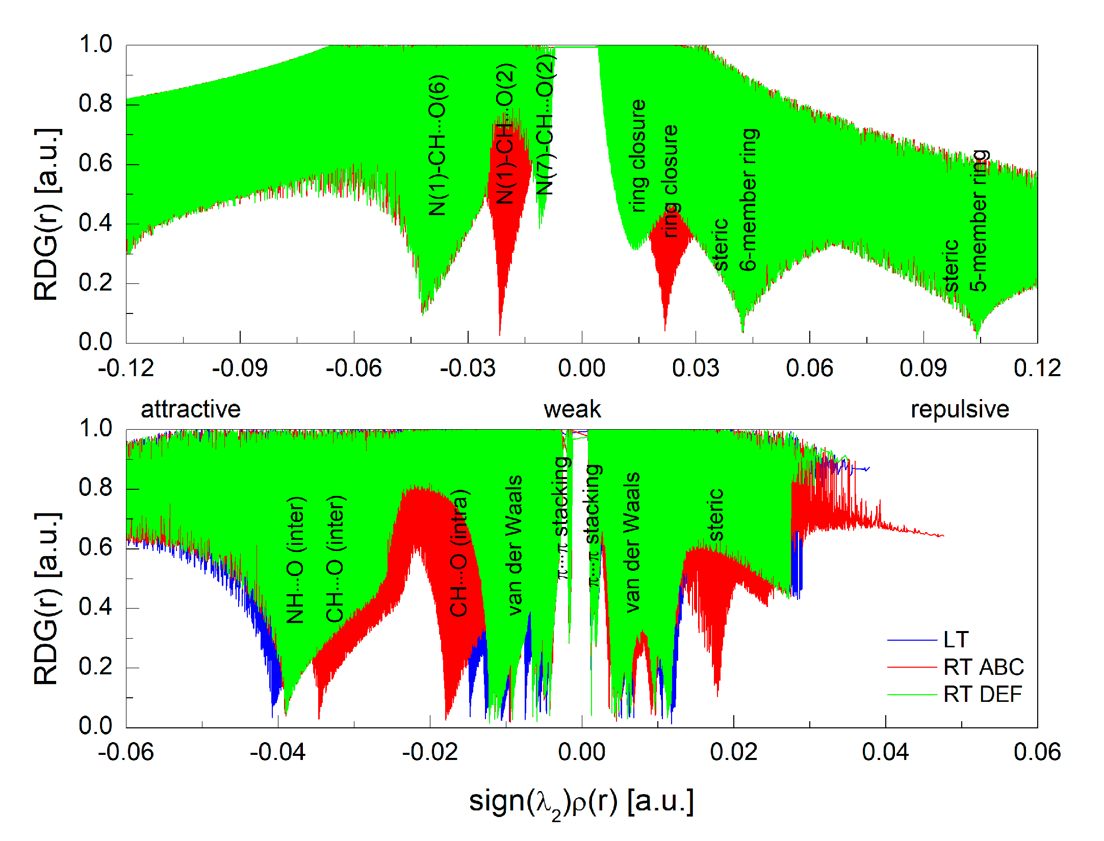
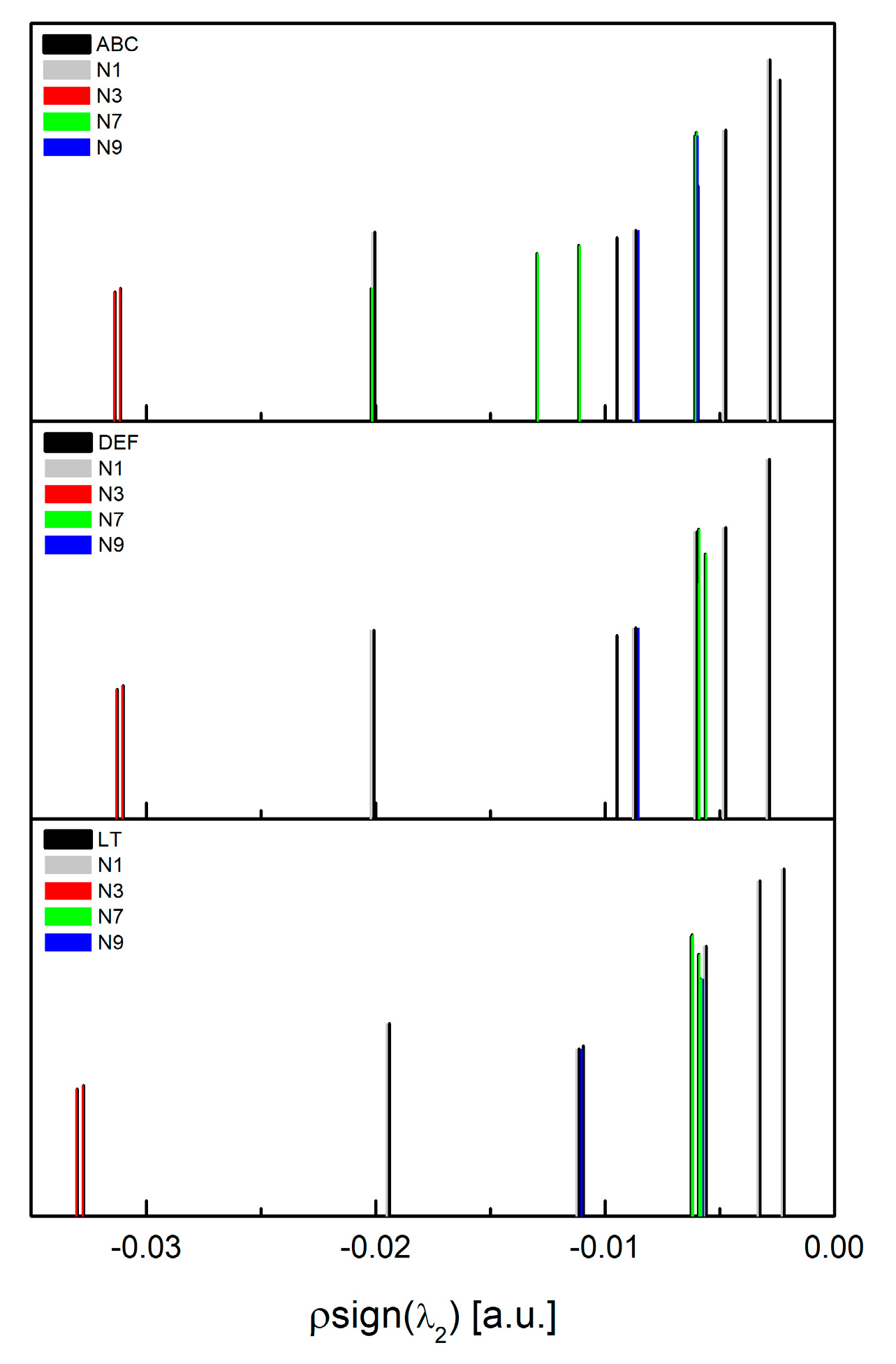
2.4. Analysis of the Topology of Interactions—Quantum Theory of Atoms in Molecules
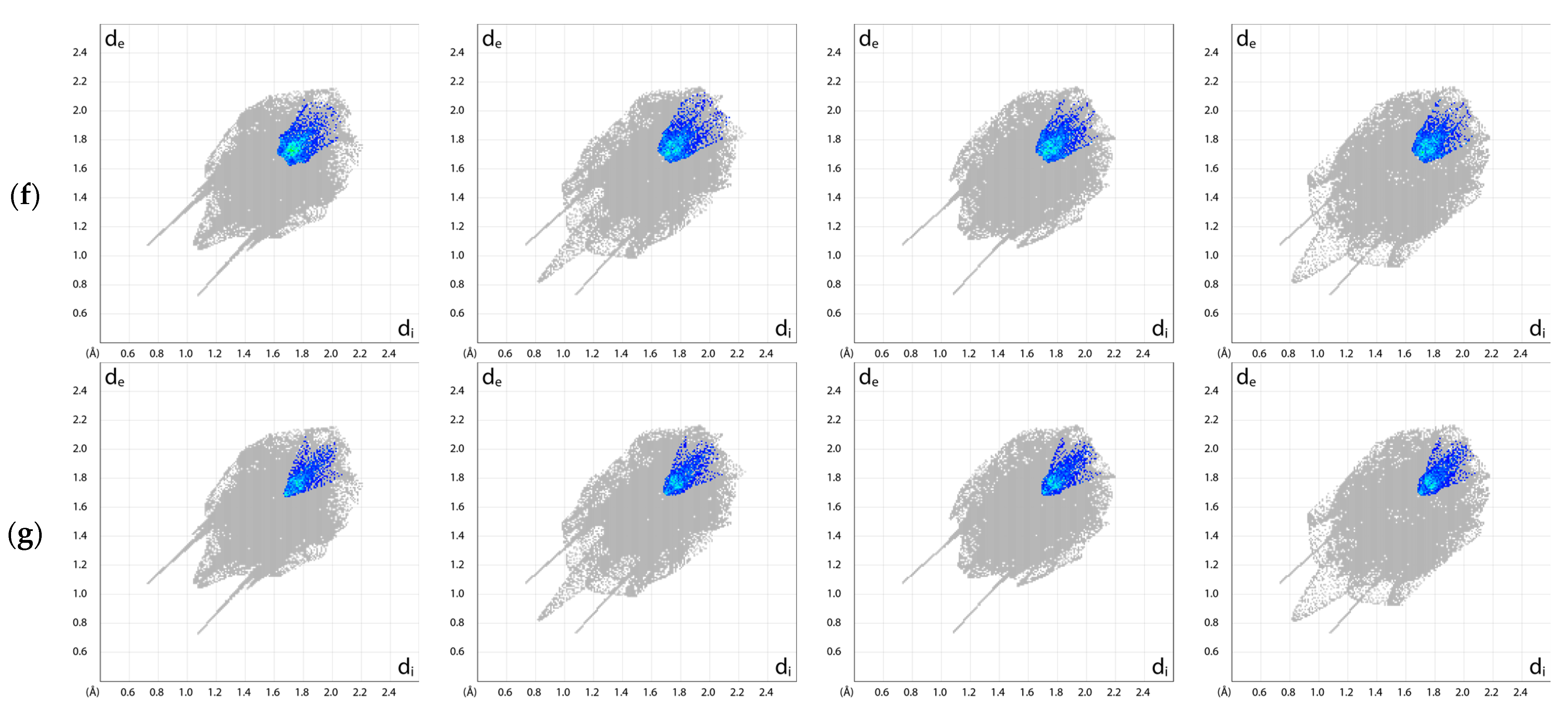
2.5. Exploration of Intermolecular Interaction Patterns—3D Hirshfeld Surface Analysis
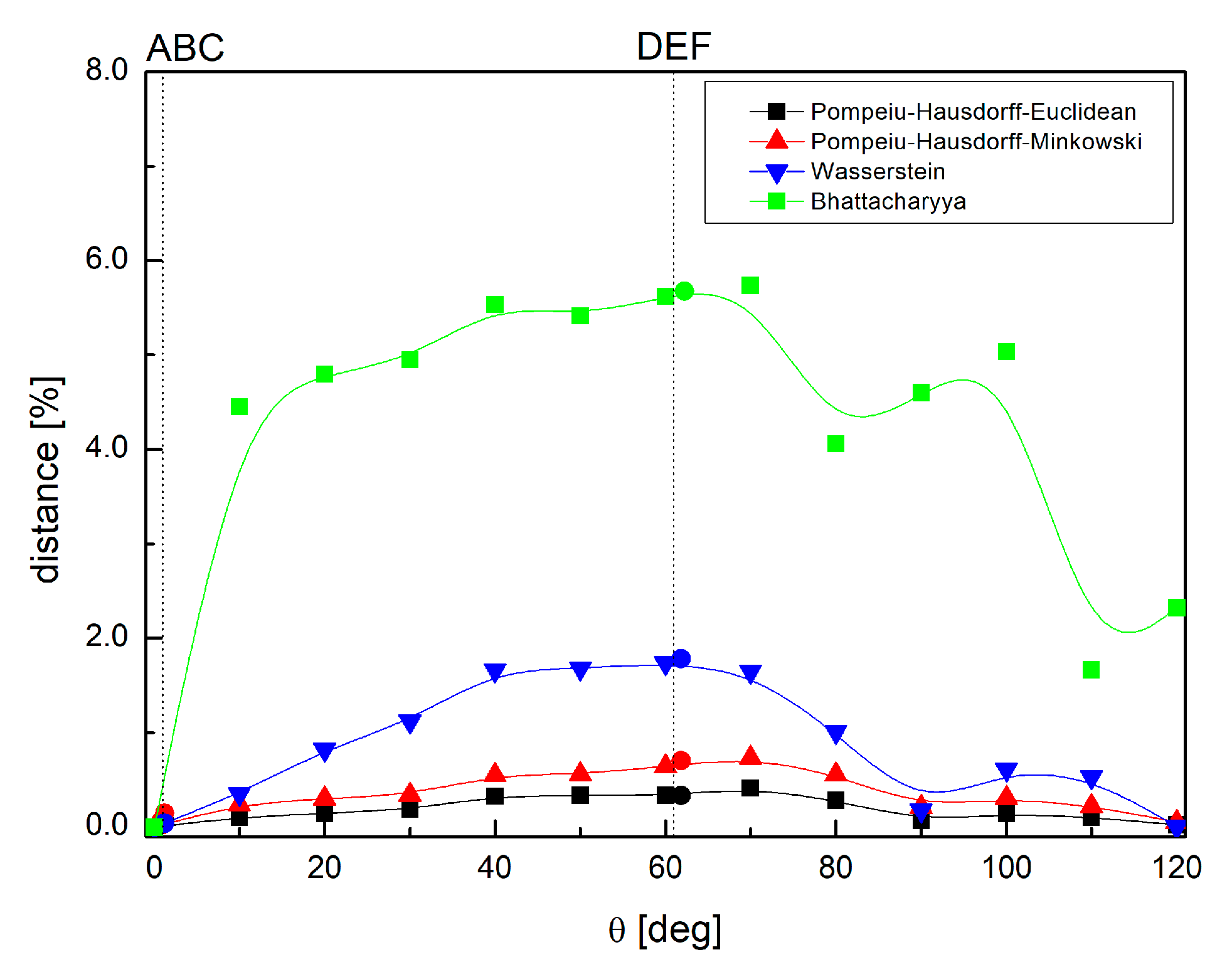
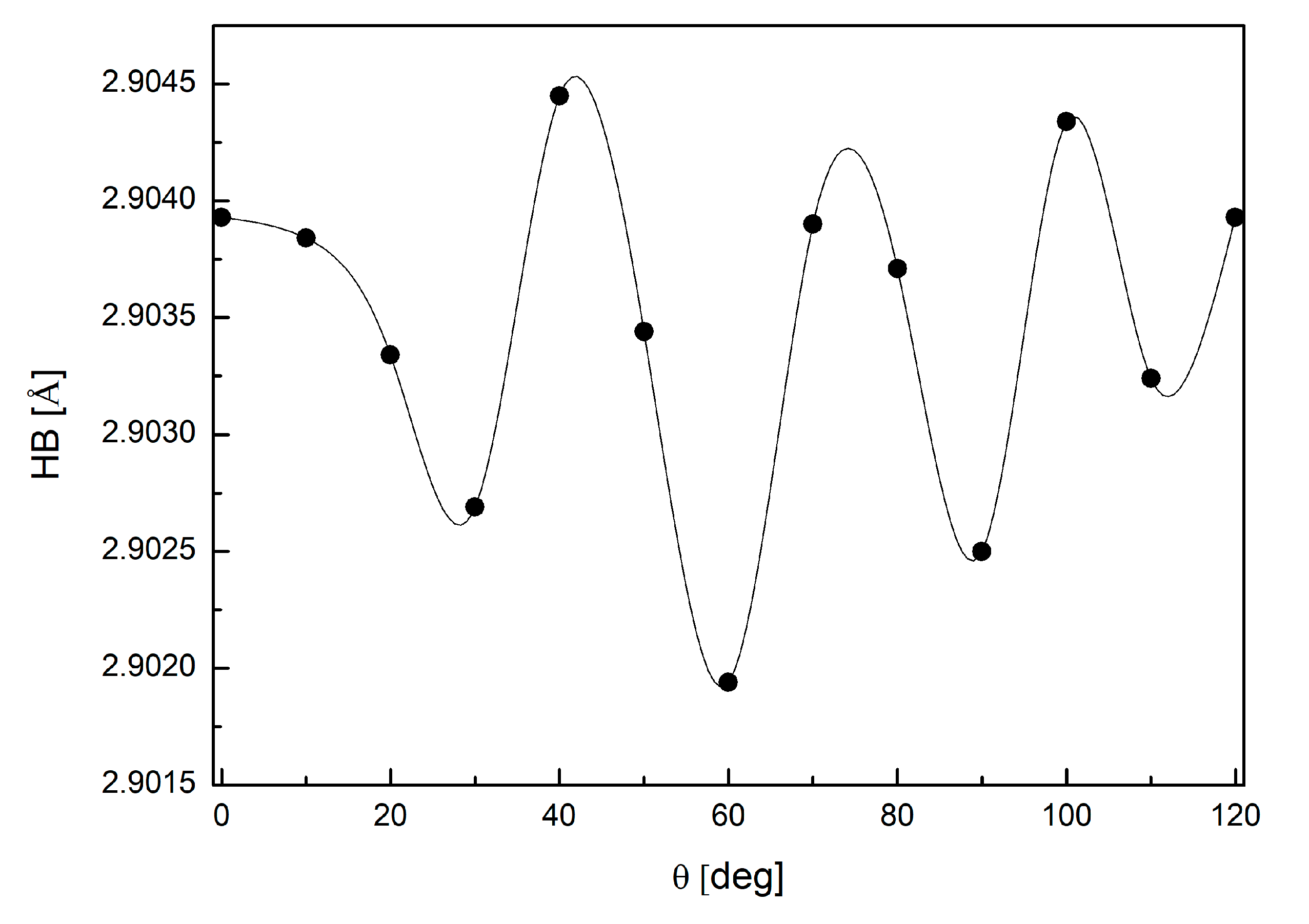
2.6. Comparison of the Differences in Interactions Patterns Due to the Methyl Group Rotation—Mathematical Metrics
- Pompeiu–Hausdorff metrics [68], which measures how far two subsets of a metric space are from each other, as in the following Equation (13):where d can be calculated as the Manhattan distance, as follows:or as the Euclidian distance, as follows:
- The Bhattacharayya coefficient [69], which is a distance between two probability distributions, as follows:
- The Wasserstein distance (Kantorovich–Rubinstein metric) [70], which is a function defined between probability distributions on a given metric space, as follows:where sup represents the supremum, inf represents the infimum, pi, qi are interactions in each structure, and dist are permutations of all pi, qi , and sum runs overall.
2.7. Exploration of Binding—Molecular Docking
3. Results and Discussion
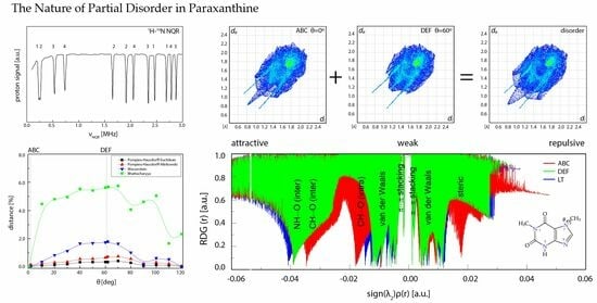
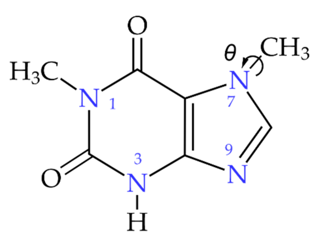
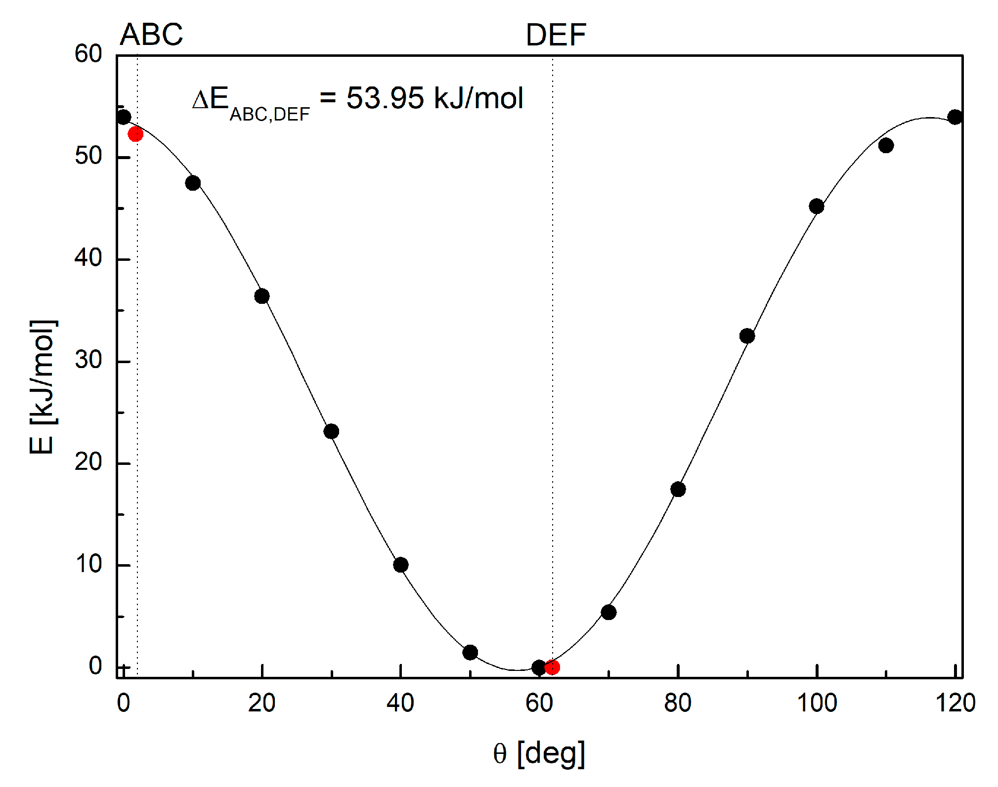
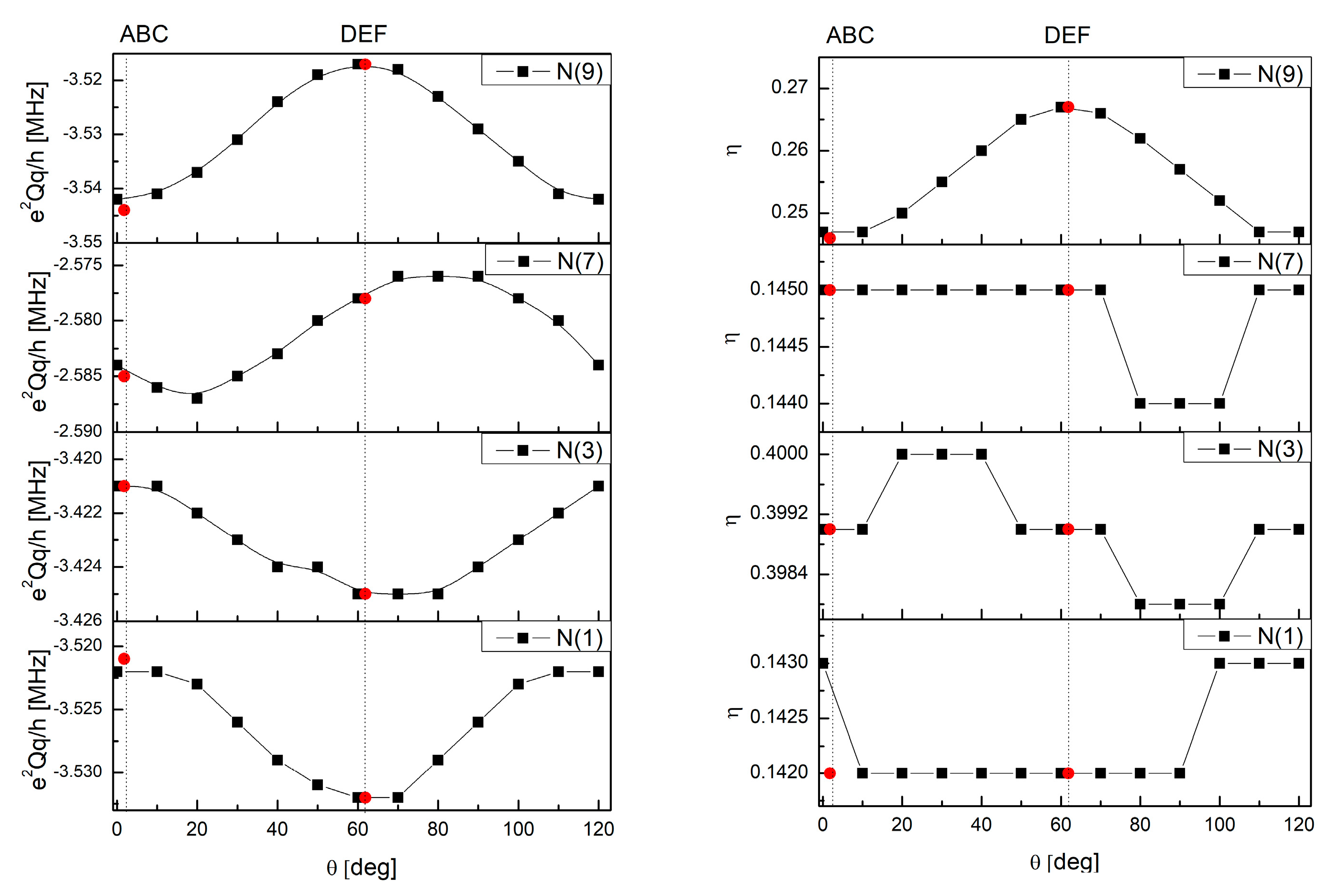
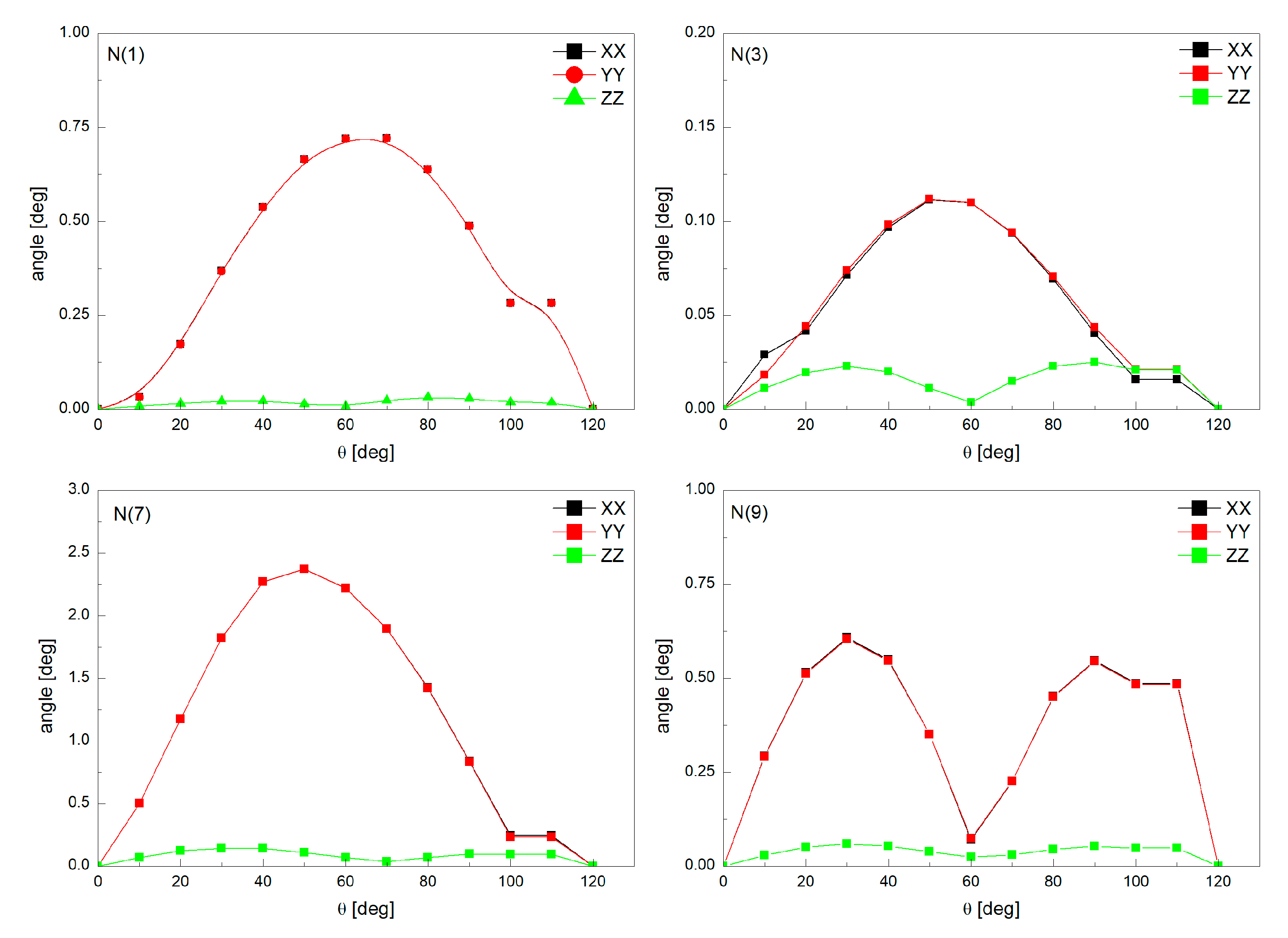
3.1. 1H-14N NQDR Spectrum
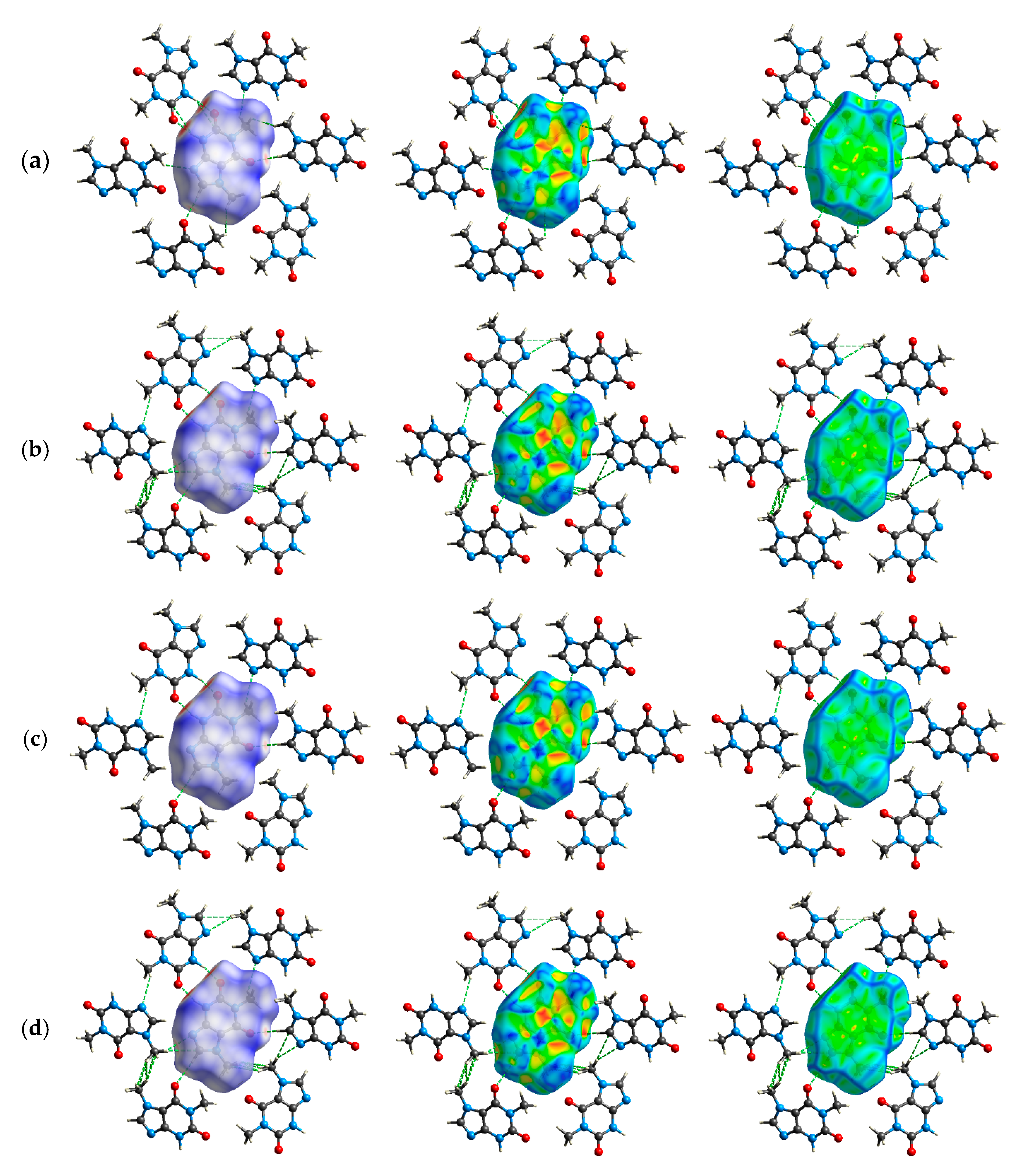
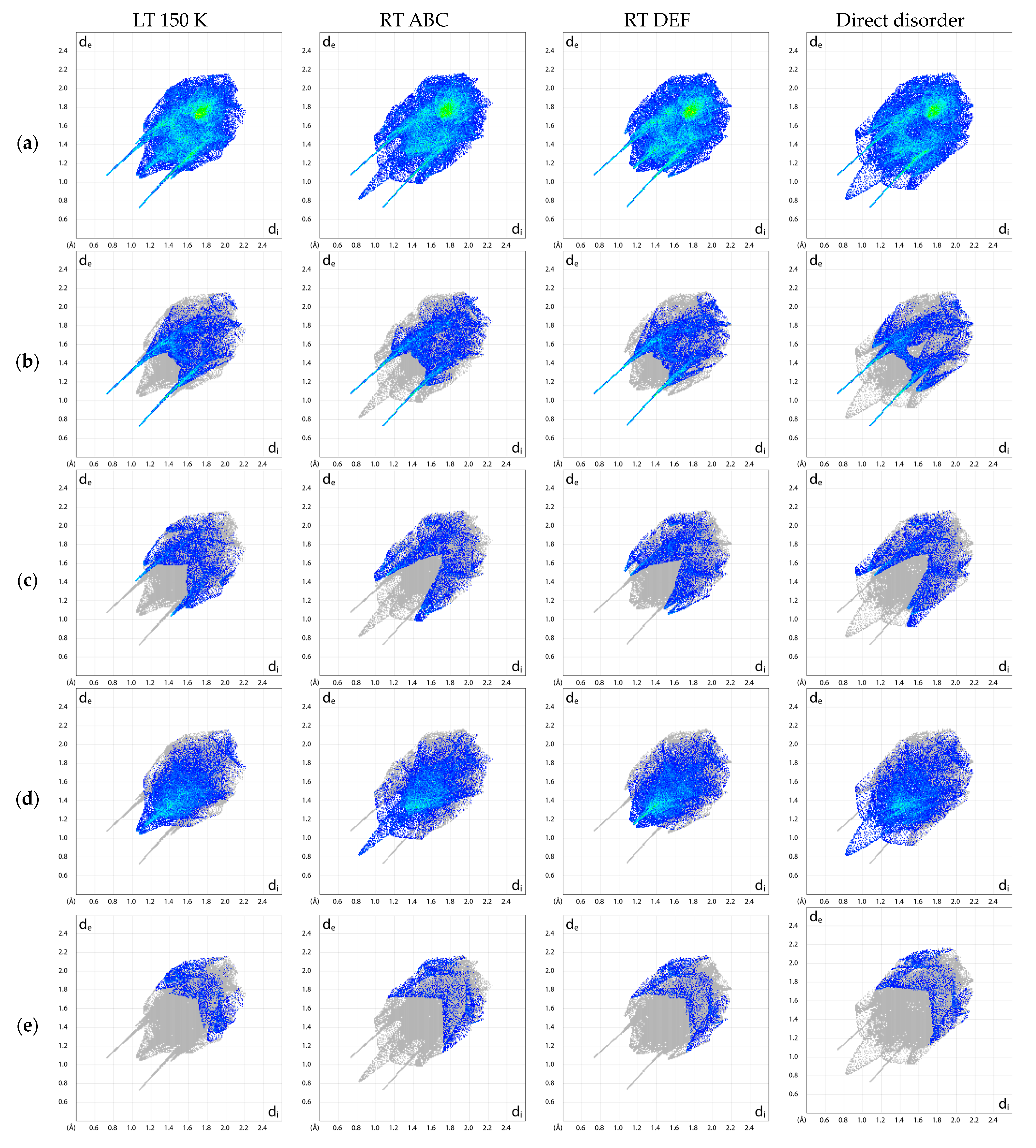
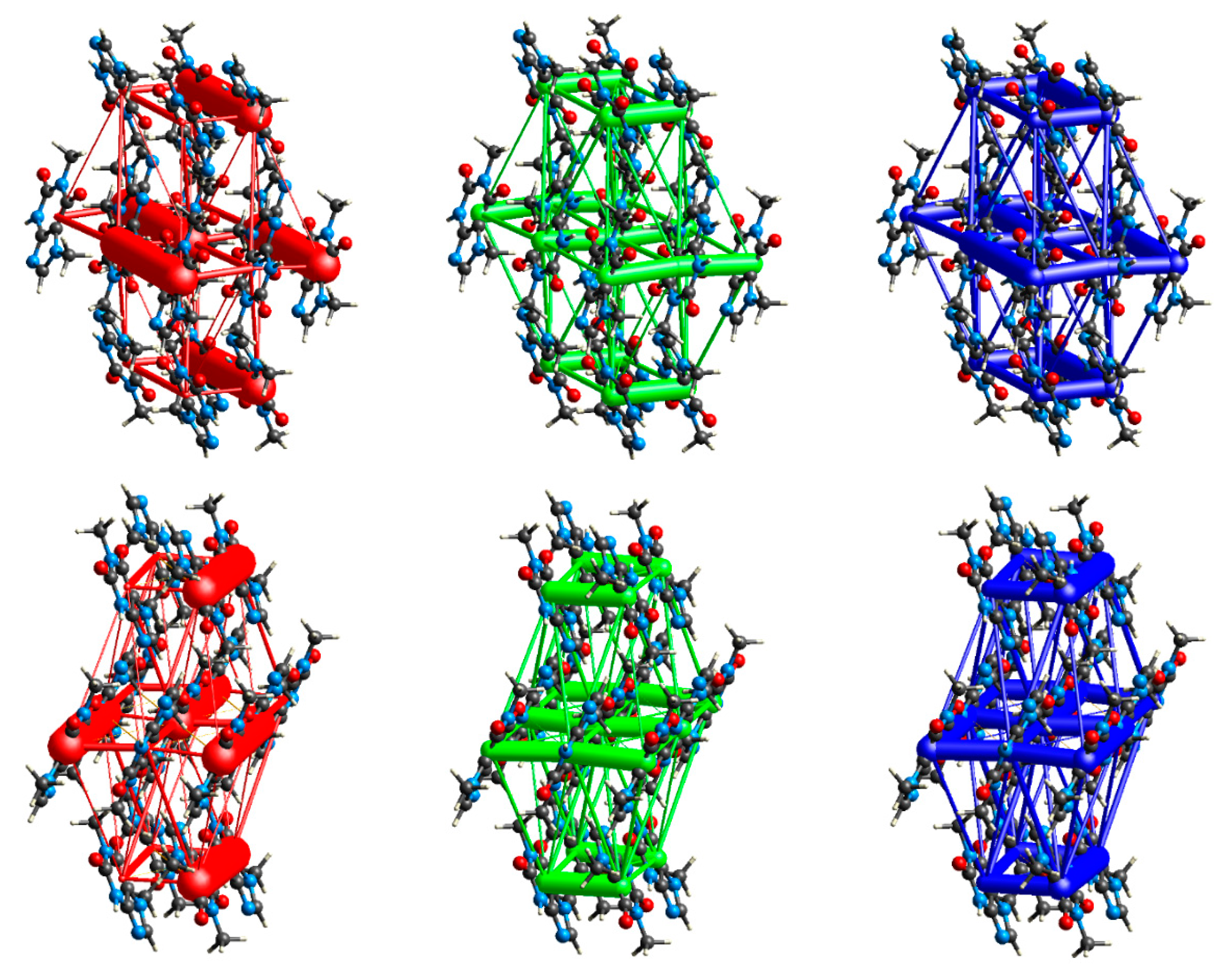
3.2. Intermolecular Interactions Pattern in Crystal
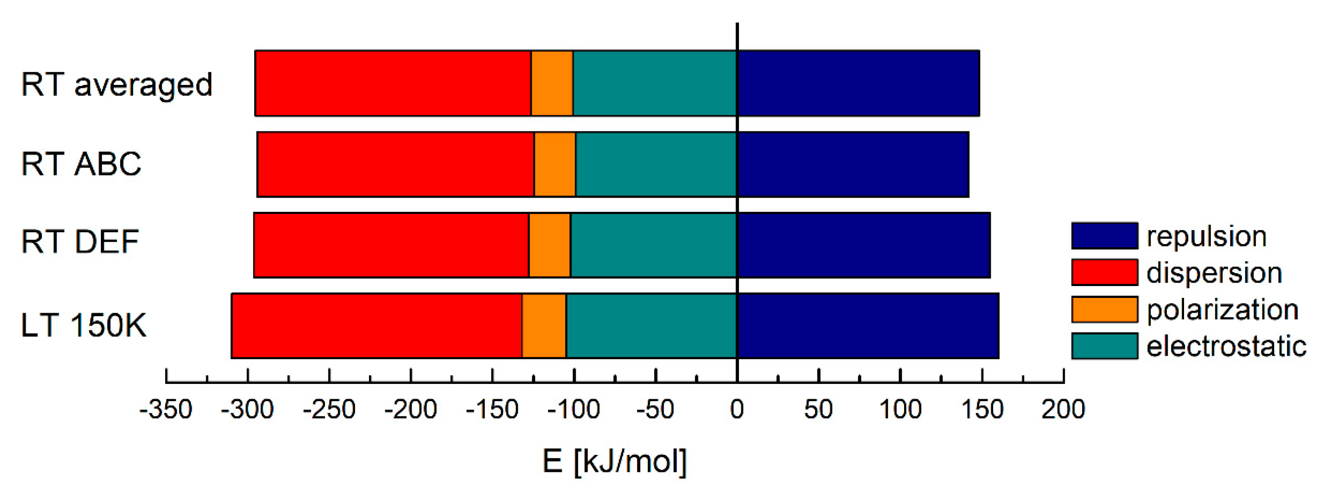
3.3. Characterization of the Strength of the Interactions
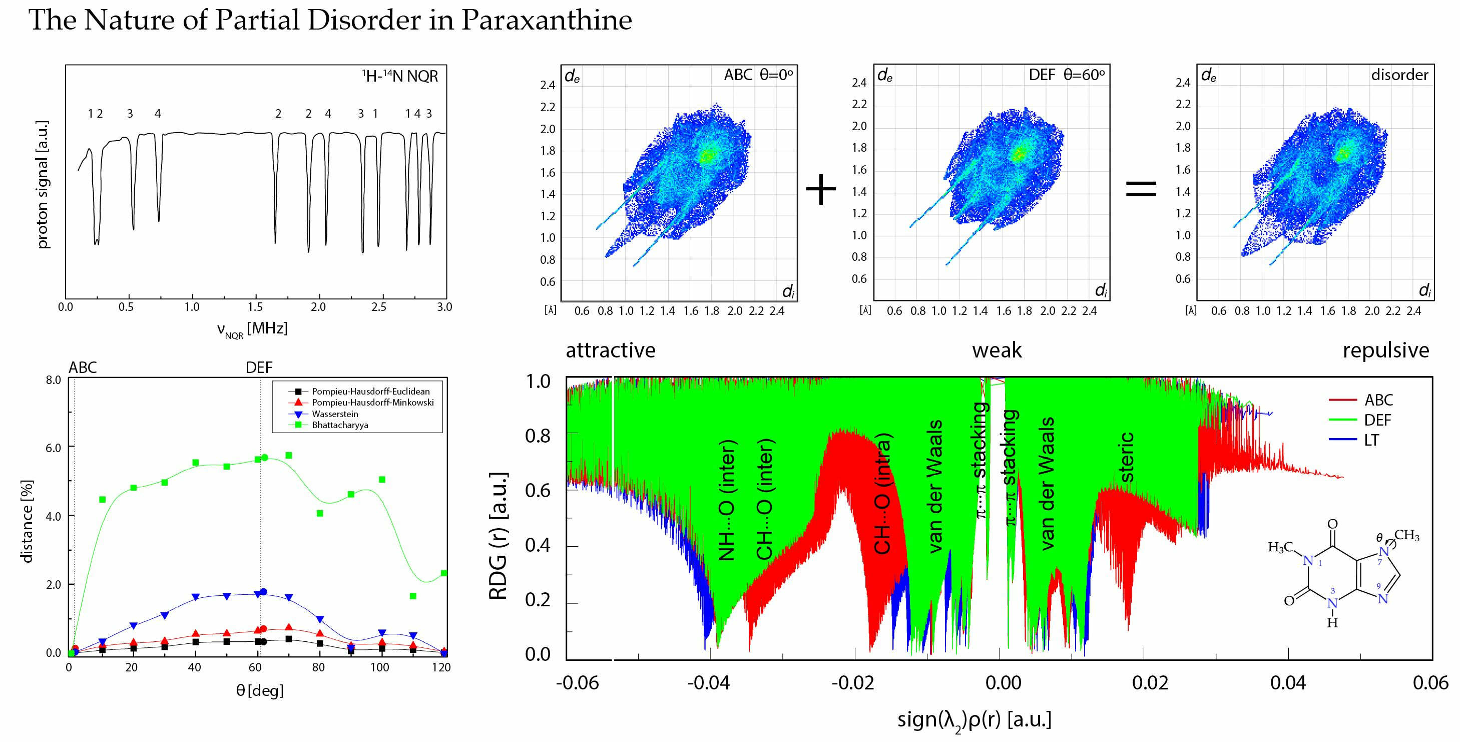
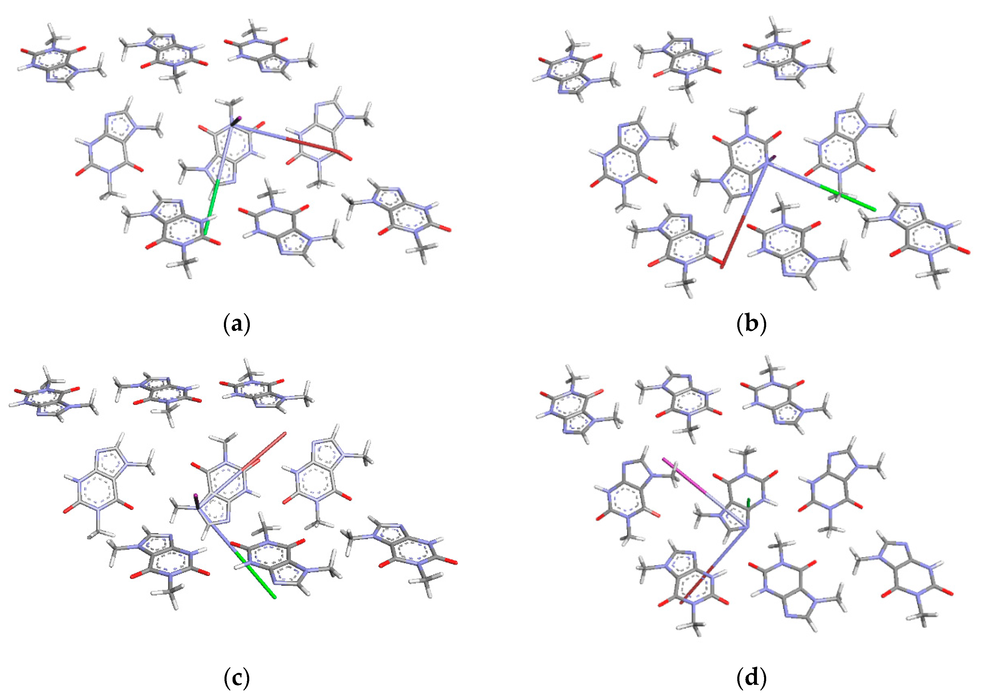
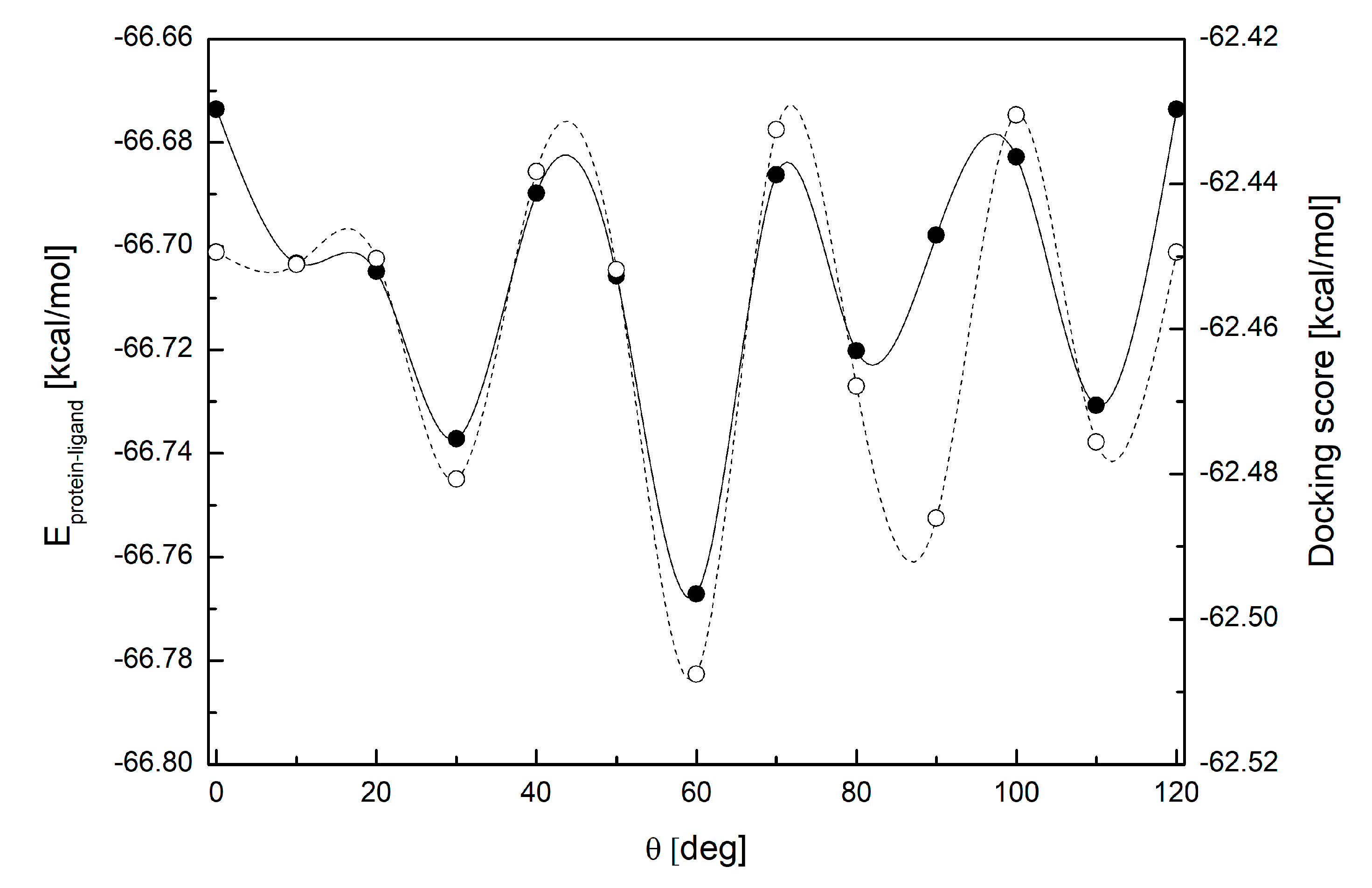
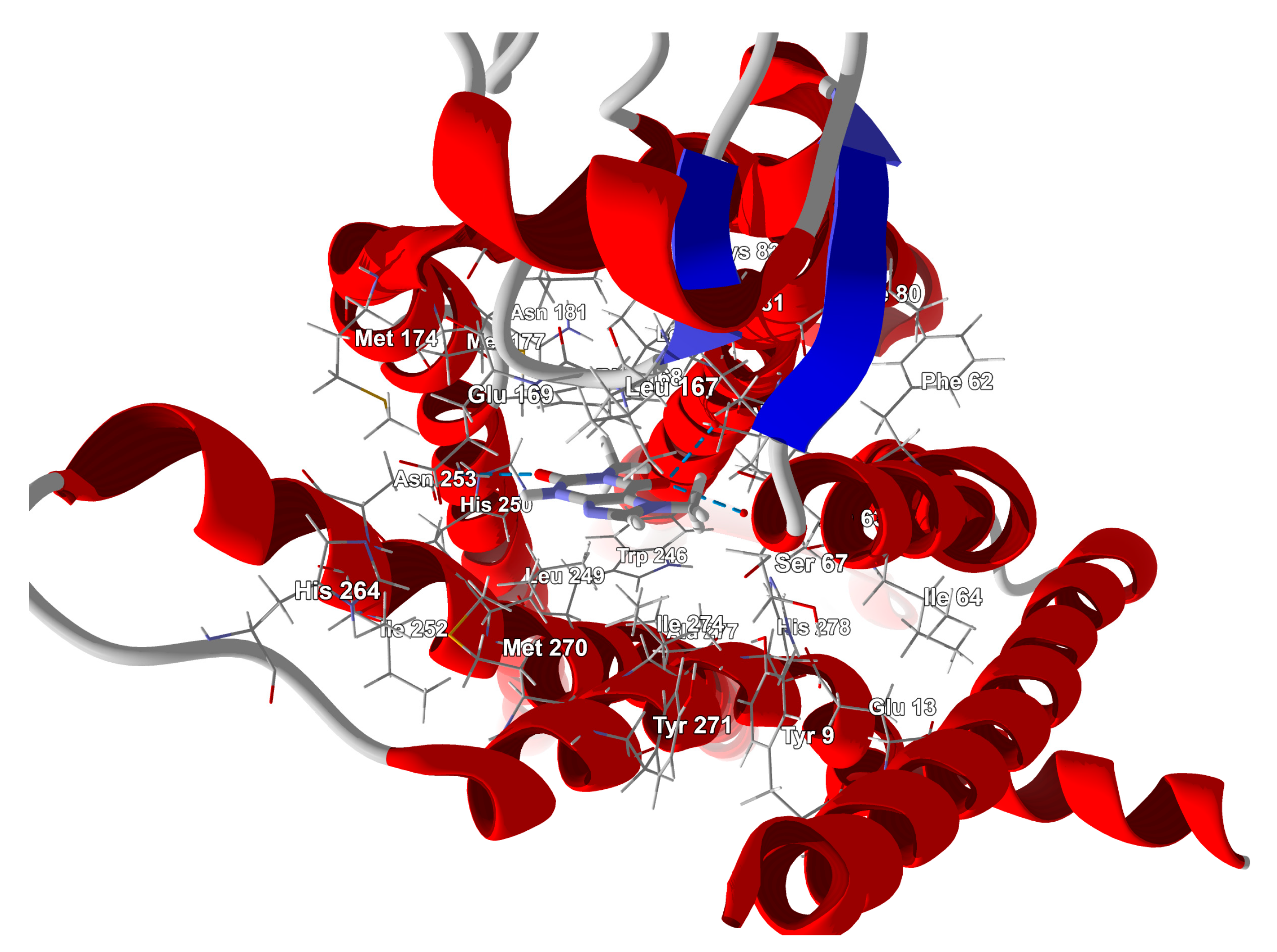
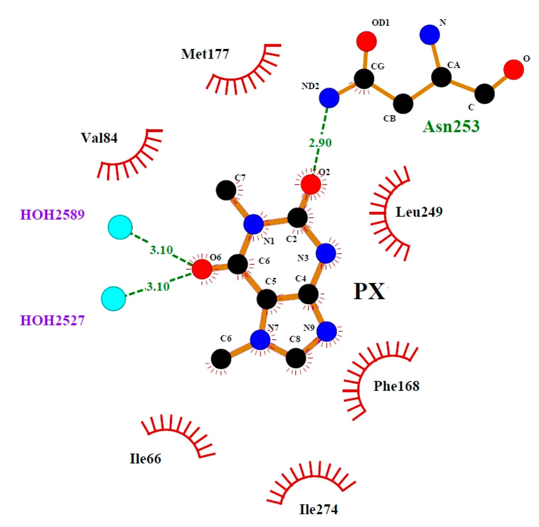
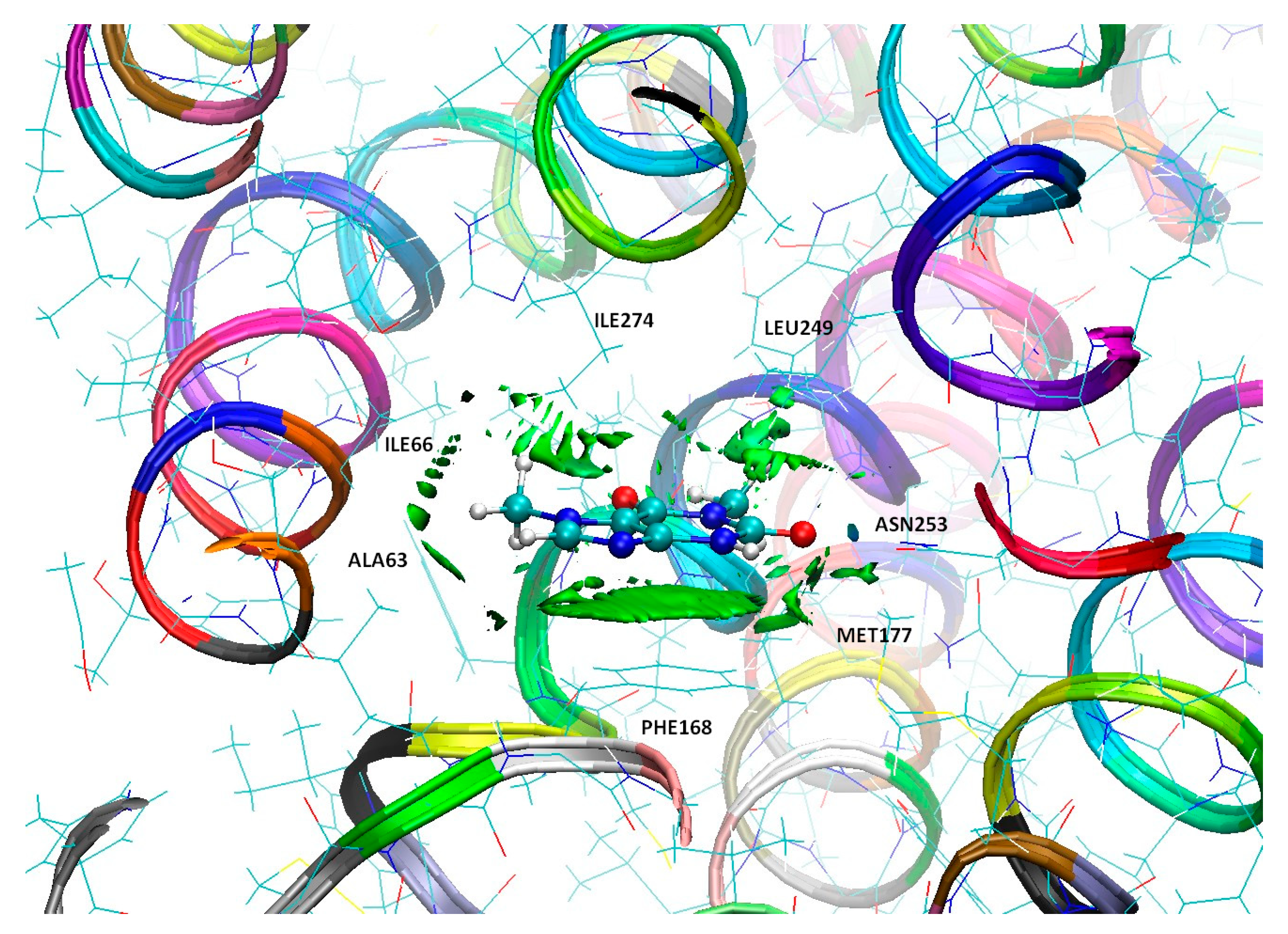
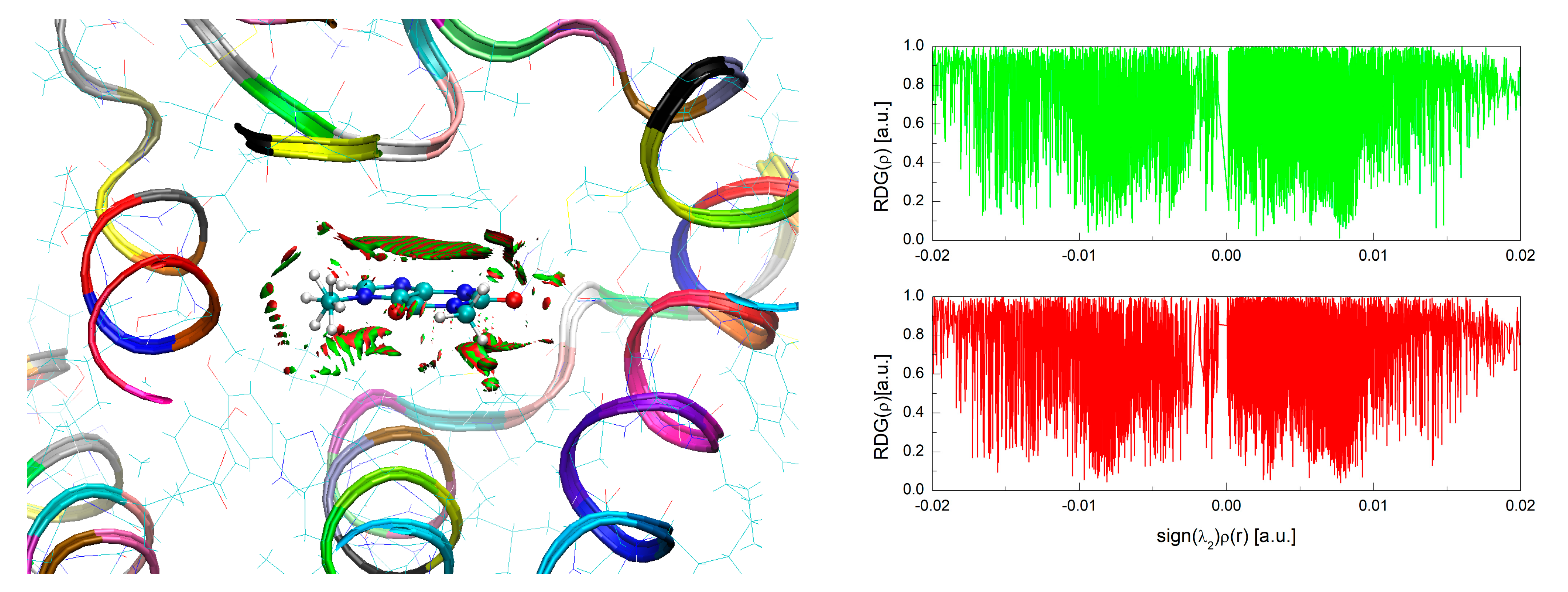
3.4. Binding Mode of Paraxanthine with A2A Receptor
4. Conclusions
Supplementary Materials
Author Contributions
Funding
Acknowledgments
Conflicts of Interest
References
- Zrenner, R.; Stitt, M.; Sonnewald, U.; Boldt, R. Pyrimidine and Purine Biosynthesis and Degradation in Plants. Annu. Rev. Plant Biol. 2006, 57, 805–836. [Google Scholar] [CrossRef]
- Monteiro, J.; Alves, M.G.; Oliveira, P.F.; Silva, B.M. Pharmacological potential of methylxanthines: Retrospective analysis and future expectations. Crit. Rev. Food Sci. Nutr. 2018, 59, 2597–2625. [Google Scholar] [CrossRef]
- Arnaud, M.J. The pharmacology of caffeine. Prog. Drug Res. 1987, 31, 273–313. [Google Scholar] [CrossRef] [PubMed]
- Orrú, M.; Guitart, X.; Karcz-Kubicha, M.; Solinas, M.; Justinova, Z.; Barodia, S.K.; Zanoveli, J.; Cortes, A.; Lluis, C.; Casado, V.; et al. Psychostimulant pharmacological profile of paraxanthine, the main metabolite of caffeine in humans. Neuropharmacology 2013, 67, 476–484. [Google Scholar] [CrossRef]
- Caffeine. In IARC Monographs on the Evaluation of Carcinogenic Risks to Humans; World Health Organization, International Agency for Research on Cancer: Lyon, France, 1991; Volume 51, pp. 291–390.
- Tassaneeyakul, W.; Birkett, D.J.; McManus, M.E.; Tassaneeyakul, W.; Veronese, M.E.; Andersson, T.; Tukey, R.H.; Miners, J.O. Caffeine metabolism by human hepatic cytochromes P450: Contributions of 1A2, 2E1 and 3A isoforms. Biochem. Pharmacol. 1994, 47, 1767–1776. [Google Scholar] [CrossRef]
- Cornelis, M.C.; El-Sohemy, A.; Campos, H. Genetic polymorphism of the adenosine A2A receptor is associated with habitual caffeine consumption. Am. J. Clin. Nutr. 2007, 86, 240–244. [Google Scholar] [CrossRef]
- Lajin, B.; Schweighofer, N.; Goessler, W.; Obermayer-Pietsch, B. The determination of the Paraxanthine/Caffeine ratio as a metabolic biomarker for CYP1A2 activity in various human matrices by UHPLC-ESIMS/MS. Talanta 2021, 234, 122658. [Google Scholar] [CrossRef] [PubMed]
- Mazzafera, P. Catabolism of caffeine in plants and microorganisms. Front. Biosci. 2004, 9, 1348. [Google Scholar] [CrossRef]
- Berthou, F.; Guillois, B.; Riche, C.; Dreano, Y.; Jacqz-Aigrain, E.; Beaune, P.H. Interspecies variations in caffeine metabolism related to cytochrome P4501A enzymes. Xenobiotica Fate Foreign Compd. Biol. Syst. 1992, 22, 671–680. [Google Scholar] [CrossRef]
- Ashihara, H.; Sano, H.; Crozier, A. Caffeine and related purine alkaloids: Biosynthesis, catabolism, function and genetic engineering. Phytochemistry 2008, 69, 841–856. [Google Scholar] [CrossRef]
- Gao, Z.-G.; Jacobson, K.A. Emerging adenosine receptor agonists. Expert Opin. Emerg. Drugs 2007, 12, 479–492. [Google Scholar] [CrossRef] [PubMed]
- Dulloo, A.G.; Seydoux, J.; Girardier, L. Paraxanthine (metabolite of caffeine) mimics caffeine’s interaction with sympathetic control of thermogenesis. Am. J. Physiol. 1994, 267 Pt 1, E801–E804. [Google Scholar] [CrossRef] [PubMed]
- Benowitz, N.L.; Jacob, P.; Mayan, H.; Denaro, C. Sympathomimetic effects of paraxanthine and caffeine in humans. Clin. Pharmacol. Ther. 1995, 58, 684–691. [Google Scholar] [CrossRef]
- Han, Y.; Xun, L.; Wang, X.; Yang, S.; Sun, Z.; Shi, H.; Xu, X.; Hu, S. Detection of caffeine and its main metabolites for early diagnosis of Parkinson’s disease using micellar electrokinetic capillary chromatography. Electrophoresis 2020, 41, 1392–1399. [Google Scholar] [CrossRef] [PubMed]
- Barr, R.G. Methylxanthines for exacerbations of chronic obstructive pulmonary disease: Meta-analysis of randomised trials. BMJ 2003, 327, 643. [Google Scholar] [CrossRef]
- Xing, D.; Yoo, C.; Gonzalez, D.; Jenkins, V.; Nottingham, K.; Dickerson, B.; Leonard, M.; Ko, J.; Faries, M.; Kephart, W.; et al. Dose-Response of Paraxanthine on Cognitive Function: A Double Blind, Placebo Controlled, Crossover Trial. Nutrients 2021, 13, 4478. [Google Scholar] [CrossRef]
- Ferré, S. An update on the mechanisms of the psychostimulant effects of caffeine. J. Neurochem. 2008, 105, 1067–1079. [Google Scholar] [CrossRef]
- Yoo, C.; Xing, D.; Gonzalez, D.; Jenkins, V.; Nottingham, K.; Dickerson, B.; Leonard, M.; Ko, J.; Faries, M.; Kephart, W.; et al. Acute Paraxanthine Ingestion Improves Cognition and Short-Term Memory and Helps Sustain Attention in a Double-Blind, Placebo-Controlled, Crossover Trial. Nutrients 2021, 13, 3980. [Google Scholar] [CrossRef]
- Ferre, S.; Orru, M.; Guitart, X. Paraxanthine: Connecting Caffeine to Nitric Oxide Neurotransmission. J. Caffeine Res. 2013, 3, 72–78. [Google Scholar] [CrossRef]
- Guerreiro, S.; Toulorge, D.; Hirsch, E.; Marien, M.; Sokoloff, P.; Michel, P.P. Paraxanthine, the primary metabolite of caffeine, provides protection against dopaminergic cell death via stimulation of ryanodine receptor channels. Mol. Pharmacol. 2008, 74, 980–989. [Google Scholar] [CrossRef]
- Costentin, J. Main neurotropic and psychotropic effects of methylxanthines (caffeine, theophylline, theobromine, paraxanthine). PSN 2010, 8, 182–186. [Google Scholar] [CrossRef]
- Mitchell, L.; MacFarlane, P.M. Mechanistic actions of oxygen and methylxanthines on respiratory neural control and for the treatment of neonatal apnea. Respir. Physiol. Neurobiol. 2020, 273, 103318. [Google Scholar] [CrossRef] [PubMed]
- Gressner, O.A.; Lahme, B.; Siluschek, M.; Gressner, A.M. Identification of paraxanthine as the most potent caffeine-derived inhibitor of connective tissue growth factor expression in liver parenchymal cells. Liver Int. 2009, 29, 886–897. [Google Scholar] [CrossRef] [PubMed]
- Sasamoto, H.; Fujii, Y.; Ashihara, H. Effect of Purine Alkaloids on the Proliferation of Lettuce Cells Derived from Protoplasts. Nat. Prod. Commun. 2015, 10, 1934578X1501000. [Google Scholar] [CrossRef]
- Razavi, S.M.; Asadi, N. Physiological and biochemical responses of lettuce plant to the allochemical compound of paraxanthine. J. Plant Process Funct. 2022, 10, 51–60. [Google Scholar]
- Hosseini, A.; Mirmahdi, E.; Moghaddam, M.A. A new strategy for treatment of Anosmia and Ageusia in COVID-19 patients. Integr. Respir. Med. 2020, 1, 2. [Google Scholar] [CrossRef]
- Khani, E.; Khiali, S.; Beheshtirouy, S.; Entezari-Maleki, T. Potential pharmacologic treatments for COVID-19 smell and taste loss: A comprehensive review. Eur. J. Pharmacol. 2021, 912, 174582. [Google Scholar] [CrossRef]
- Kohli, P.; Soler, Z.M.; Nguyen, S.A.; Muus, J.S.; Schlosser, R.J. The Association Between Olfaction and Depression: A Systematic Review. Chem. Senses 2016, 41, 479–486. [Google Scholar] [CrossRef]
- Alharbi, O.; Xu, Y.; Goodacre, R. Simultaneous multiplexed quantification of caffeine and its major metabolites theobromine and paraxanthine using surface-enhanced Raman scattering. Anal. Bioanal. Chem. 2015, 407, 8253–8261. [Google Scholar] [CrossRef]
- Seliger, J.; Zagar, V.; Apih, T.; Gregorovic, A.; Latosińska, M.; Olejniczak, G.A.; Latosińska, J.N. Polymorphism and disorder in natural active ingredients. Low and high-temperature phases of anhydrous caffeine: Spectroscopic (1H-14N NMR-NQR/14N NQR) and solid-state computational modelling (DFT/QTAIM/RDS) study. Eur. J. Pharm. Sci. 2016, 85, 18–30. [Google Scholar] [CrossRef]
- Latosińska, J.N.; Latosińska, M.; Olejniczak, G.A.; Seliger, J.; Zagar, V. Topology of the interactions pattern in pharmaceutically relevant polymorphs of methylxanthines (caffeine, theobromine, and theophiline): Combined experimental (1H-14N nuclear quadrupole double resonance) and computational (DFT and Hirshfeld-based) study. J. Chem. Inf. Model. 2014, 54, 2570–2584. [Google Scholar] [CrossRef] [PubMed]
- Yalkowsky, S.H.; He, Y.; Jain, P. Handbook of Aqueous Solubility Data; CRC Press: Boca Raton, FL, USA, 2016; p. 1620. [Google Scholar]
- Carlucci, L.; Gavezzotti, A. Molecular Recognition and Crystal Energy Landscapes: An X-ray and Computational Study of Caffeine and Other Methylxanthines. Chem.—A Eur. J. 2005, 11, 271–279. [Google Scholar] [CrossRef]
- Echeverría, J.; Aullón, G.; Alvarez, S. Dihydrogen intermolecular contacts in group 13 compounds: H⋯H or E⋯H (E = B, Al, Ga) interactions? Dalton Trans. 2017, 46, 2844–2854. [Google Scholar] [CrossRef] [PubMed]
- Rösel, S.; Quanz, H.; Logemann, C.; Becker, J.; Mossou, E.; Cañadillas-Delgado, L.; Caldeweyher, E.; Grimme, S.; Schreiner, P.R. London Dispersion Enables the Shortest Intermolecular Hydrocarbon H⋯H Contact. J. Am. Chem. Soc. 2017, 139, 7428–7431. [Google Scholar] [CrossRef] [PubMed]
- Hajji, M.; Al-Otaibi, J.S.; Belkhiria, M.; Dhifaoui, S.; Habib, M.A.; Elmgirhi, S.M.H.; Mtiraoui, H.; Bel-Hadj-Tahar, R.; Msaddek, M.; Guerfel, T. Structural and computational analyses of a 2-propanolammonium-chlorocadmate(II) assembly: Pivotal role of hydrogen bonding and H–H interactions. J. Mol. Struct. 2021, 1223, 128998. [Google Scholar] [CrossRef]
- Latosińska, J.N.; Latosińska, M.; Orzeszko, A.; Maurin, J.K. Synthesis and Crystal Structure of Adamantylated 4,5,6,7-Tetrahalogeno-1H-benzimidazoles Novel Multi-Target Ligands (Potential CK2, M2 and SARS-CoV-2 Inhibitors); X-ray/DFT/QTAIM/Hirshfeld Surfaces/Molecular Docking Study. Molecules 2022, 28, 147. [Google Scholar] [CrossRef]
- Latosińska, J.N.; Latosińska, M.; Seliger, J.; Žagar, V.; Apih, T.; Grieb, P. Elucidating the Role of Noncovalent Interactions in Favipiravir, a Drug Active against Various Human RNA Viruses; a 1H-14N NQDR/Periodic DFT/QTAIM/RDS/3D Hirshfeld Surfaces Combined Study. Molecules 2023, 28, 3308. [Google Scholar] [CrossRef]
- Latosińska, J.N. NQR parameters: Electric field gradient tensor and asymmetry parameter studied in terms of density functional theory. Int. J. Quantum Chem. 2003, 91, 284–296. [Google Scholar] [CrossRef]
- Bader, R. Atoms in Molecules: A Quantum Theory (International Series of Monographs on Chemistry); Oxford University Press: New York, NY, USA, 1994. [Google Scholar]
- Johnson, E.R.; Keinan, S.; Mori-Sánchez, P.; Contreras-García, J.; Cohen, A.J.; Yang, W. Revealing Noncovalent Interactions. J. Am. Chem. Soc. 2010, 132, 6498–6506. [Google Scholar] [CrossRef]
- Spackman, M.A.; Jayatilaka, D. Hirshfeld surface analysis. CrystEngComm 2009, 11, 19. [Google Scholar] [CrossRef]
- Spackman, M.A.; McKinnon, J.J. Fingerprinting intermolecular interactions in molecular crystalsBased on the presentation given at CrystEngComm Discussion, 29th June 1st July 2002, Bristol, UK. CrystEngComm 2002, 4, 378. [Google Scholar] [CrossRef]
- Kohn, W.; Sham, L.J. Self-Consistent Equations Including Exchange and Correlation Effects. Phys. Rev. 1965, 140, A1133–A1138. [Google Scholar] [CrossRef]
- Levy, M. Universal variational functionals of electron densities, first-order density matrices, and natural spin-orbitals and solution of the v-representability problem. Proc. Natl. Acad. Sci. USA 1979, 76, 6062–6065. [Google Scholar] [CrossRef] [PubMed]
- Zhao, Y.; Truhlar, D.G. The M06 suite of density functionals for main group thermochemistry, thermochemical kinetics, noncovalent interactions, excited states, and transition elements: Two new functionals and systematic testing of four M06-class functionals and 12 other functionals. Theor. Chem. Acc. 2007, 120, 215–241. [Google Scholar] [CrossRef]
- Latosińska, J.N.; Koput, J. Analysis of the NQR parameters in 2-nitro-5-methylimidazole derivatives by quantum chemical calculations. Phys. Chem. Chem. Phys. 2000, 2, 145–150. [Google Scholar] [CrossRef]
- Frisch, M.J.; Trucks, G.W.; Schlegel, H.B.; Scuseria, G.E.; Robb, M.A.; Cheeseman, J.R.; Scalmani, G.; Barone, V.; Petersson, G.A.; Nakatsuji, H.; et al. Gaussian 16 Rev. C.01; Gaussian, Inc.: Wallingford, CT, USA, 2016. [Google Scholar]
- Zhang, Y.; Yang, W. Comment on “Generalized Gradient Approximation Made Simple”. Phys. Rev. Lett. 1998, 80, 890. [Google Scholar] [CrossRef]
- Perdew, J.P.; Burke, K.; Ernzerhof, M. Generalized Gradient Approximation Made Simple. Phys. Rev. Lett. 1996, 77, 3865–3868. [Google Scholar] [CrossRef]
- Wu, Z.; Cohen, R.E. More accurate generalized gradient approximation for solids. Phys. Rev. B 2006, 73, 235116. [Google Scholar] [CrossRef]
- Perdew, J.P.; Ruzsinszky, A.; Csonka, G.I.; Vydrov, O.A.; Scuseria, G.E.; Constantin, L.A.; Zhou, X.; Burke, K. Restoring the Density-Gradient Expansion for Exchange in Solids and Surfaces. Phys. Rev. Lett. 2008, 100, 136406. [Google Scholar] [CrossRef]
- Perdew, J.P.; Chevary, J.A.; Vosko, S.H.; Jackson, K.A.; Pederson, M.R.; Singh, D.J.; Fiolhais, C. Atoms, molecules, solids, and surfaces: Applications of the generalized gradient approximation for exchange and correlation. Phys. Rev. B 1992, 46, 6671–6687, Erratum in Phys. Rev. B 1993, 48, 4978. [Google Scholar] [CrossRef]
- Tkatchenko, A.; Scheffler, M. Accurate Molecular Van Der Waals Interactions from Ground-State Electron Density and Free-Atom Reference Data. Phys. Rev. Lett. 2009, 102, 073005. [Google Scholar] [CrossRef] [PubMed]
- Peng, H.; Yang, Z.H.; Perdew, J.P.; Sun, J. Versatile van der Waals Density Functional Based on a Meta-Generalized Gradient Approximation. Phys. Rev. X 2016, 6, 041005. [Google Scholar] [CrossRef]
- Sun, J.; Ruzsinszky, A.; Perdew, J.P. Strongly Constrained and Appropriately Normed Semilocal Density Functional. Phys. Rev. Lett. 2015, 115, 036402. [Google Scholar] [CrossRef]
- Bartók, A.P.; Yates, J.R. Regularized SCAN functional. J. Chem. Phys. 2019, 150, 161101. [Google Scholar] [CrossRef]
- Pyykkö, P. Year-2008 nuclear quadrupole moments. Mol. Phys. 2008, 106, 1965–1974. [Google Scholar] [CrossRef]
- Abramov, Y.A. On the Possibility of Kinetic Energy Density Evaluation from the Experimental Electron-Density Distribution. Acta Crystallogr. Sect. A Found. Crystallogr. 1997, 53, 264–272. [Google Scholar] [CrossRef]
- Espinosa, E.; Molins, E.; Lecomte, C. Hydrogen bond strengths revealed by topological analyses of experimentally observed electron densities. Chem. Phys. Lett. 1998, 285, 170–173. [Google Scholar] [CrossRef]
- Mata, I.; Alkorta, I.; Espinosa, E.; Molins, E. Relationships between interaction energy, intermolecular distance and electron density properties in hydrogen bonded complexes under external electric fields. Chem. Phys. Lett. 2011, 507, 185–189. [Google Scholar] [CrossRef]
- Emamian, S.; Lu, T.; Kruse, H.; Emamian, H. Exploring Nature and Predicting Strength of Hydrogen Bonds: A Correlation Analysis Between Atoms-in-Molecules Descriptors, Binding Energies, and Energy Components of Symmetry-Adapted Perturbation Theory. J. Comput. Chem. 2019, 40, 2868–2881. [Google Scholar] [CrossRef]
- Afonin, A.V.; Vashchenko, A.V.; Sigalov, M.V. Estimating the energy of intramolecular hydrogen bonds from 1H NMR and QTAIM calculations. Org. Biomol. Chem. 2016, 14, 11199–11211. [Google Scholar] [CrossRef]
- Nikolaienko, T.Y.; Bulavin, L.A.; Hovorun, D.M. Bridging QTAIM with vibrational spectroscopy: The energy of intramolecular hydrogen bonds in DNA-related biomolecules. Phys. Chem. Chem. Phys. 2012, 14, 7441. [Google Scholar] [CrossRef] [PubMed]
- Humphrey, W.; Dalke, A.; Schulten, K. VMD: Visual molecular dynamics. J. Mol. Graph. 1996, 14, 33–38. [Google Scholar] [CrossRef]
- Jelsch, C.; Ejsmont, K.; Huder, L. The enrichment ratio of atomic contacts in crystals, an indicator derived from the Hirshfeld surface analysis. IUCrJ 2014, 1, 119–128. [Google Scholar] [CrossRef] [PubMed]
- Hausdorff, F. Grundzüge der Mengenlehre; Leipzig Viet; Gerstein-University of Toronto: Toronto, ON, Canada, 1914. [Google Scholar]
- Bhattacharyya, A. On a Measure of Divergence between Two Multinomial Populations. Sankhyā Indian J. Stat. (1933–1960) 1946, 7, 401–406. [Google Scholar]
- Vaserstein, L.N. Markov processes on countable space products describing large systems of automata. Probl. Inform. Transm. 1969, 5, 47–52. [Google Scholar]
- Latosińska, J.N.; Latosińska, M.; Szafrański, M.; Seliger, J.; Žagar, V.; Burchardt, D.V. Impact of structural differences in carcinopreventive agents indole-3-carbinol and 3,3′-diindolylmethane on biological activity. An X-ray, 1H–14N NQDR, 13C CP/MAS NMR, and periodic hybrid DFT study. Eur. J. Pharm. Sci. 2015, 77, 141–153. [Google Scholar] [CrossRef]
- Trott, O.; Olson, A.J. AutoDock Vina: Improving the speed and accuracy of docking with a new scoring function, efficient optimization, and multithreading. J. Comput. Chem. 2009, 31, 455–461. [Google Scholar] [CrossRef]
- Eberhardt, J.; Santos-Martins, D.; Tillack, A.F.; Forli, S. AutoDock Vina 1.2.0: New Docking Methods, Expanded Force Field, and Python Bindings. J. Chem. Inf. Model. 2021, 61, 3891–3898. [Google Scholar] [CrossRef]
- Wallace, A.C.; Laskowski, R.A.; Thornton, J.M. LIGPLOT: A program to generate schematic diagrams of protein-ligand interactions. Protein Eng. Des. Sel. 1995, 8, 127–134. [Google Scholar] [CrossRef]
- Laskowski, R.A.; Swindells, M.B. LigPlot+: Multiple Ligand–Protein Interaction Diagrams for Drug Discovery. J. Chem. Inf. Model. 2011, 51, 2778–2786. [Google Scholar] [CrossRef]
- Seliger, J.; Žagar, V.; Blinc, R. 1H-14N Nuclear Quadrupole Double Resonance with Multiple Frequency Sweeps. Z. Naturforschung A 1994, 49, 31–34. [Google Scholar] [CrossRef]
- Seliger, J.; Zagar, V.; Blinc, R. A New Highly Sensitive 1H-14N Nuclear-Quadrupole Double-Resonance Technique. J. Magn. Reson. 1994, 106, 214–222. [Google Scholar] [CrossRef]
- Etter, M.C. Encoding and decoding hydrogen-bond patterns of organic compounds. Acc. Chem. Res. 2002, 23, 120–126. [Google Scholar] [CrossRef]
- Gilli, G.; Gilli, P. The Nature of the Hydrogen Bond: Outline of a Comprehensive Hydrogen Bond Theory, 1st ed.; Oxford Academic: Oxford, UK, 2009. [Google Scholar]
- Koch, U.; Popelier, P.L.A. Characterization of C-H-O Hydrogen Bonds on the Basis of the Charge Density. J. Phys. Chem. 2002, 99, 9747–9754. [Google Scholar] [CrossRef]
- Cheng, R.K.Y.; Segala, E.; Robertson, N.; Deflorian, F.; Doré, A.S.; Errey, J.C.; Fiez-Vandal, C.; Marshall, F.H.; Cooke, R.M. Structures of Human A 1 and A 2A Adenosine Receptors with Xanthines Reveal Determinants of Selectivity. Structure 2017, 25, 1275–1285.e4. [Google Scholar] [CrossRef]


| Nitrogen Site | ν+ [MHz] | ν− [MHz] | ν0 [MHz] | e2qQ/h [MHz] | η | Final Assignment * |
|---|---|---|---|---|---|---|
| N(1) | 2.685 | 2.457 | 0.228 | −3.428 | 0.133 | >N(1)CH3 |
| N(4) | 2.780 | 2.047 | 0.733 | −3.218 | 0.456 | >N(3)H |
| N(2) | 1.910 | 1.650 | 0.260 | −2.373 | 0.219 | >N(7)CH3 |
| N(3) | 2.870 | 2.340 | 0.530 | −3.473 | 0.305 | -N(9)= |
| Structure | Site | ν+ [MHz] | ν− [MHz] | ν0 [MHz] | e2qQ/h [MHz] | η | s, r2, Intercept, Slope |
|---|---|---|---|---|---|---|---|
| LT 150 K protons optimized | >N(1)CH3 | 2.696 | 2.556 | 0.140 | −3.501 | 0.08 | 0.052 |
| >N(3)H | 2.799 | 2.027 | 0.772 | −3.217 | 0.48 | 0.995 | |
| >N(7)CH3 | 2.019 | 1.767 | 0.252 | −2.524 | 0.20 | 0.016 | |
| -N(9)= | 2.785 | 2.388 | 0.397 | −3.449 | 0.23 | 1.002 | |
| RT ABC protons optimized | >N(1)CH3 | 2.675 | 2.553 | 0.122 | −3.485 | 0.07 | 0.073 |
| >N(3)H | 2.809 | 2.021 | 0.789 | −3.22 | 0.49 | 0.993 | |
| >N(7)CH3 | 2.017 | 1.777 | 0.240 | −2.529 | 0.19 | −0.041 | |
| -N(9)= | 2.776 | 2.381 | 0.395 | −3.438 | 0.23 | 1.027 | |
| RT DEF protons optimized | >N(1)CH3 | 2.696 | 2.556 | 0.140 | −3.501 | 0.08 | 0.063 |
| >N(3)H | 2.799 | 2.027 | 0.772 | −3.217 | 0.48 | 0.994 | |
| >N(7)CH3 | 2.019 | 1.767 | 0.252 | −2.524 | 0.20 | −0.038 | |
| -N(9)= | 2.785 | 2.388 | 0.397 | −3.449 | 0.23 | 1.027 | |
| RT ABCDEF averaged protons optimized | >N(1)CH3 | 2.685 | 2.554 | 0.131 | −3.493 | 0.08 | −0.039 |
| >N(3)H | 2.804 | 2.024 | 0.780 | −3.219 | 0.49 | 1.027 | |
| >N(7)CH3 | 2.018 | 1.772 | 0.246 | −2.527 | 0.20 | 0.068 | |
| -N(9)= | 2.781 | 2.385 | 0.396 | −3.444 | 0.23 | 0.994 | |
| direct disorder protons optimized | >N(1)CH3 | 2.884 | 2.734 | 0.150 | −3.745 | 0.08 | 9.365 |
| >N(3)H | 2.989 | 1.806 | 1.183 | −3.197 | 0.74 | 0.391 | |
| >N(7)CH3 | 4.709 | 2.866 | 1.843 | −5.050 | 0.73 | 0.781 | |
| -N(9)= | 2.518 | 2.102 | 0.416 | −3.080 | 0.27 | 0.822 |
| Site | ν+ [MHz] | ν− [MHz] | ν0 [MHz] | e2qQ/h [MHz] | η | s, r2, Intercept, Slope | |
|---|---|---|---|---|---|---|---|
| LT 150 K | >N(1)CH3 | 2.835 | 2.511 | 0.324 | −3.564 | 0.182 | 0.104 |
| >N(3)H | 2.878 | 2.113 | 0.765 | −3.327 | 0.460 | 0.989 | |
| >N(7)CH3 | 1.929 | 1.723 | 0.206 | −2.435 | 0.169 | 0.025 | |
| -N(9)= | 2.707 | 2.189 | 0.517 | −3.264 | 0.317 | 0.995 | |
| RT ABC | >N(1)CH3 | 2.765 | 2.517 | 0.248 | −3.521 | 0.141 | 0.064 |
| >N(3)H | 2.907 | 2.225 | 0.682 | −3.421 | 0.399 | 0.994 | |
| >N(7)CH3 | 2.033 | 1.844 | 0.189 | −2.585 | 0.146 | −0.041 | |
| -N(9)= | 2.876 | 2.440 | 0.436 | −3.544 | 0.246 | 1.057 | |
| RT DEF | >N(1)CH3 | 2.774 | 2.524 | 0.251 | −3.532 | 0.142 | 0.058 |
| >N(3)H | 2.910 | 2.227 | 0.683 | −3.425 | 0.399 | 0.994 | |
| >N(7)CH3 | 2.027 | 1.840 | 0.187 | −2.578 | 0.145 | −0.033 | |
| -N(9)= | 2.873 | 2.403 | 0.470 | −3.517 | 0.267 | 1.052 | |
| RT ABCDEF averaged | >N(1)CH3 | 2.769 | 2.520 | 0.250 | −3.522 | 0.142 | 0.046 |
| >N(3)H | 2.908 | 2.226 | 0.683 | −3.423 | 0.415 | 0.995 | |
| >N(7)CH3 | 2.030 | 1.842 | 0.188 | −2.541 | 0.144 | −0.036 | |
| -N(9)= | 2.874 | 2.422 | 0.453 | −3.491 | 0.265 | 1.054 |
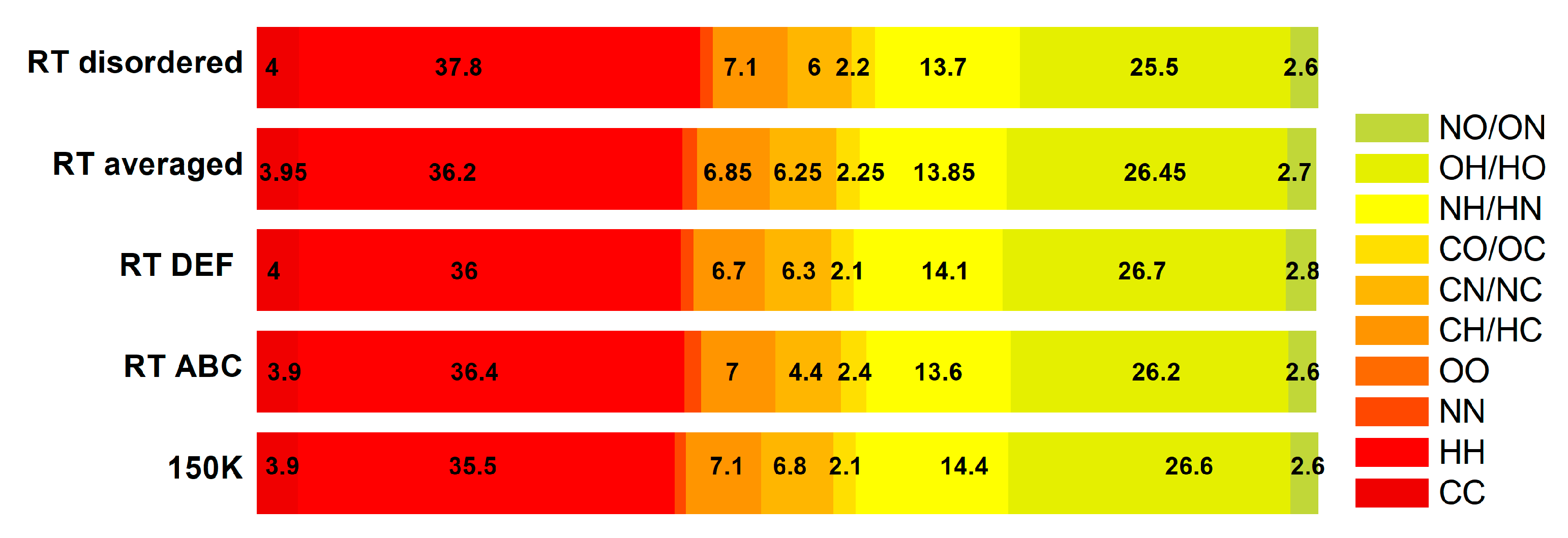
| Structure | Homonuclear | Heteronuclear | ||||||||
|---|---|---|---|---|---|---|---|---|---|---|
| CC | HH | NN | OO | CH | CN | CO | NH | OH | NO | |
| LT 150 K | 3.9 | 35.5 | 1.1 | 0 | 7.1 | 6.8 | 2.1 | 14.4 | 26.6 | 2.6 |
| RT ABC | 3.9 | 36.4 | 1.6 | 0 | 7 | 6.2 | 2.4 | 13.6 | 26.2 | 2.6 |
| RT DEF | 4 | 36 | 1.2 | 0 | 6.7 | 6.3 | 2.1 | 14.1 | 26.7 | 2.8 |
| RT ABCDEF averaged | 3.95 | 36.2 | 1.4 | 0 | 6.85 | 6.25 | 2.25 | 13.85 | 26.45 | 2.7 |
| RT disorder | 4 | 37.8 | 1.2 | 0 | 7.1 | 6.0 | 2.2 | 13.7 | 25.5 | 2.6 |
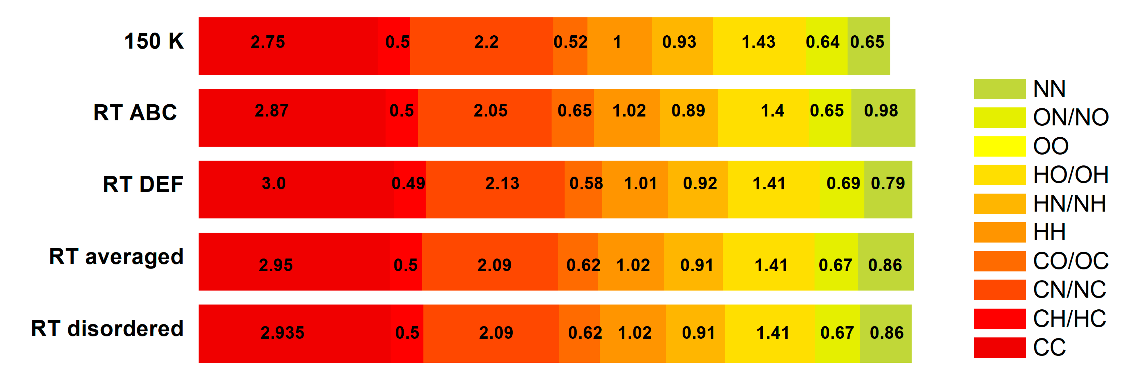
| Structure | Atom | C | H | N | O |
|---|---|---|---|---|---|
| LT 150 K | Surface% | 11.9 | 59.55 | 13.0 | 15.65 |
| C | 2.75 | - | - | - | |
| H | 0.50 | 1.00 | - | - | |
| N | 2.20 | 0.93 | 0.65 | - | |
| O | 0.52 | 1.43 | 0.64 | 0 | |
| RT ABC | Surface% | 11.8 | 59.8 | 12.8 | 15.6 |
| C | 2.87 | ||||
| H | 0.50 | 1.02 | |||
| N | 2.05 | 0.89 | 0.98 | ||
| O | 0.65 | 1.40 | 0.65 | 0 | |
| RT DEF | Surface% | 11.55 | 59.75 | 12.8 | 15.8 |
| C | 3.00 | ||||
| H | 0.49 | 1.01 | |||
| N | 2.13 | 0.92 | 0.73 | ||
| O | 0.58 | 1.41 | 0.69 | 0 | |
| RT ABCDEF averaged | Surface% | 11.68 | 59.78 | 12.80 | 15.70 |
| C | 2.94 | - | - | - | |
| H | 0.50 | 1.02 | - | - | |
| N | 2.09 | 0.91 | 0.86 | - | |
| O | 0.62 | 1.41 | 0.67 | 0 | |
| RT disordered | Surface% | 11.65 | 60.95 | 12.35 | 15.15 |
| C | 2.95 | - | - | - | |
| H | 0.50 | 1.02 | - | - | |
| N | 2.09 | 0.91 | 0.79 | - | |
| O | 0.62 | 1.38 | 0.69 | 0 |
| Structure | Contact Type | –N(1)= | –N(3)= | –N(7) | N(9) | Contact Type | =O(4) | =O(2) | Contact Type | C (N(1) CH3) | C N(7) CH3 | Contact Type | CH3 (N(1)) | CH3 (N(7)) |
|---|---|---|---|---|---|---|---|---|---|---|---|---|---|---|
| LT 150 K | N⋯C | 88.2 | 48.7 | 79.6 | 50.4 | O⋯C | 30.5 | 24.9 | C⋯C | 0 | 0 | H⋯C | 6.8 | 0.7 |
| N⋯H | 11.8 | 49.5 | 20.0 | 48.0 | O⋯H | 65.7 | 75.1 | C⋯H | 88.9 | 87.9 | H⋯H | 42.9 | 57.1 | |
| N⋯O | 0 | 1.8 | 0 | 1.6 | O⋯O | 0 | 0 | C⋯O | 0 | 0.5 | H⋯O | 21.4 | 21.4 | |
| N⋯N | 0 | 0 | 0.4 | 0 | O⋯N | 3.8 | 0 | C⋯N | 11.1 | 11.7 | H⋯N | 21.5 | 13.5 | |
| RT ABC | N⋯C | 87.3 | 48.6 | 79.9 | 50.8 | O⋯C | 29.4 | 24.7 | C⋯C | 0 | 0 | H⋯C | 6.3 | 0.2 |
| N⋯H | 12.7 | 50 | 19.9 | 47.8 | O⋯H | 67 | 75 | C⋯H | 89.2 | 88.6 | H⋯H | 44.8 | 55.4 | |
| N⋯O | 0 | 1.3 | 0 | 1.4 | O⋯O | 0 | 0 | C⋯O | 0 | 0.2 | H⋯O | 20.5 | 22.4 | |
| N⋯N | 0 | 0.1 | 0.1 | 0 | O⋯N | 3.6 | 0.3 | C⋯N | 10.8 | 11.2 | H⋯N | 21.1 | 13.6 | |
| RT DEF | N⋯C | 87.3 | 48.6 | 79.6 | 50.3 | O⋯C | 30.4 | 24.8 | C⋯C | 0 | 0 | H⋯C | 6.4 | 0.9 |
| N⋯H | 12.7 | 49.7 | 20.4 | 48.3 | O⋯H | 65.6 | 74.8 | C⋯H | 89.1 | 88.1 | H⋯H | 43.7 | 56.5 | |
| N⋯O | 0 | 1.7 | 0 | 1.4 | O⋯O | 0 | 0.4 | C⋯O | 0 | 0.3 | H⋯O | 20.8 | 22.1 | |
| N⋯N | 0 | 0 | 0 | 0 | O⋯N | 4 | 0 | C⋯N | 10.9 | 11.7 | H⋯N | 21.8 | 13.1 | |
| RT ABCDEF averaged | N⋯C | 87.3 | 48.6 | 79.8 | 50.6 | O⋯C | 29.9 | 24.8 | C⋯C | 0.0 | 0.0 | H⋯C | 6.4 | 0.6 |
| N⋯H | 12.7 | 49.9 | 20.2 | 48.1 | O⋯H | 66.3 | 74.9 | C⋯H | 89.2 | 88.4 | H⋯H | 44.3 | 56.0 | |
| N⋯O | 0.0 | 1.5 | 0.0 | 1.4 | O⋯O | 0.0 | 0.2 | C⋯O | 0.0 | 0.3 | H⋯O | 20.7 | 22.3 | |
| N⋯N | 0.0 | 0.1 | 0.1 | 0.0 | O⋯N | 3.8 | 0.2 | C⋯N | 10.9 | 11.5 | H⋯N | 21.5 | 13.4 |
| Hydrogen Bond | Parameter | LT 150 K | RT ABC | RT DEF |
|---|---|---|---|---|
| N(3)–H⋯O(2) | dnorm | −0.6156 | −0.6012 | −0.5994 |
| Shape index | −0.9788 | −0.9781 | −0.9800 | |
| Curvedness | −1.8587 | −1.6237 | −1.6267 | |
| C(8)–H⋯O(6) | dnorm | −0.1792 | −0.1258 | −0.1200 |
| Shape index | −0.9536 | −0.8976 | −0.9133 | |
| Curvedness | −1.8293 | −1.8489 | −1.8332 | |
| C–H⋯O(2) | dnorm | 0.1752 | 0.3293 | 0.2277 |
| Shape index | −0.1031 | −0.2422 | −0.6734 | |
| Curvedness | −2.6470 | −2.5477 | −2.7226 | |
| C–H⋯N(9) | dnorm | −0.019 | −0.052 | −0.098 |
| Shape index | −0.8637 | −0.8101 | −0.4796 | |
| Curvedness | −1.8697 | −1.8412 | −2.0382 | |
| C–H⋯O(6) | dnorm | −0.0753 | −0.0569 | −0.0612 |
| Shape index | −0.9330 | −0.7467 | −0.9141 | |
| Curvedness | −1.4493 | −1.3704 | −1.3276 |
| Structure | Ee [kJ/mol] | Ep [kJ/mol] | Ed [kJ/mol] | Er [kJ/mol] | Etotal [kJ/mol] |
|---|---|---|---|---|---|
| LT 150 K | −105.00 | −27.00 | −177.80 | 160.30 | −186.65 |
| RT ABC | −102.15 | −25.75 | −168.45 | 154.75 | −178.35 |
| RT DEF | −99.20 | −25.45 | −169.65 | 141.65 | −183.95 |
| RT averaged | −100.68 | −25.60 | −169.05 | 148.20 | −181.15 |
| Structure | Interaction Type and Their Number | Ee [kJ/mol] | Ep [kJ/mol] | Ed [kJ/mol] | Er [kJ/mol] | Et [kJ/mol] | |
|---|---|---|---|---|---|---|---|
| LT 150 K | N(3)H⋯O(2) | 2 | −87.7 | −19.6 | −14.3 | 92.6 | −62.4 |
| C(8)–H⋯O(6) | 1 | −10.8 | −3.0 | −11.6 | 14.5 | −14.8 | |
| (N7)C–H⋯O(6) + N(7)C–H⋯H–CN(7) | 2 | −17.3 | −5.4 | −16.7 | 16.0 | −26.9 | |
| N(9)⋯HC(8) v N(9)⋯H–CN(7) | 1 | −4.7 | −2.2 | −11.3 | 7.2 | −11.9 | |
| N(3)CH⋯N(9) | 1 | −6.3 | −1.8 | −10.8 | 11.5 | −10.2 | |
| N(1)CH⋯O(6) + N(1)CH⋯HCN(1) | 1 + 1 | −4.4 | −1.8 | −7.2 | 3.9 | −9.8 | |
| π⋯π stacking | 1 | −8.4 | −2.8 | −63.2 | 35.2 | −44.3 | |
| π⋯π stacking | 1 | −17.9 | −2.9 | −58.2 | 33.7 | −51.0 | |
| RT ABC | N(3)H⋯O(2) | 2 | −84.5 | −18.8 | −13.9 | 86.0 | −62.3 |
| C(8)–H⋯O(6) | 1 | −8.4 | −2.2 | −10.1 | 8.3 | −14.2 | |
| (N7)C–H⋯O(6) +N(7)C–H⋯H–CN(7) | 2 | −17.6 | −5.7 | −15.8 | 33.3 | −16 | |
| N(9)⋯HC(8) v N(9)⋯H–CN(7) | 1 | −7.3 | −2.8 | −11.5 | 14.4 | −10.9 | |
| N(3)CH⋯N(9) | 1 | −4.5 | −1.5 | −9.9 | 7.9 | −9.6 | |
| N(1)CH⋯O(6) + N(1)CH⋯HCN(1) | 1 + 1 | −4.2 | −1.6 | −6.5 | 3.1 | −9.4 | |
| π⋯π stacking | 1 | −12.5 | −3.0 | −61.2 | 32.4 | −48.8 | |
| π⋯π stacking | 1 | −14.2 | −2.4 | −54.4 | 29.0 | −46.3 | |
| RT DEF | N(3)H⋯O(2) | 2 | −84.3 | −18.8 | −13.9 | 85.6 | −62.3 |
| C(8)–H⋯O(6) | 1 | −9.2 | −2.6 | −11.0 | 10.6 | −14.6 | |
| (N7)C–H⋯O(6) + N(7)C–H⋯H–CN(7) | 2 | −17.7 | −5.3 | −16.2 | 14.7 | −27.8 | |
| N(9)⋯HC(8) v N(9)⋯H–CN(7) | 1 | −4.0 | −2.1 | −10.6 | 6.6 | −10.9 | |
| N(3)CH⋯N(9) | 1 | −4.5 | −1.5 | −9.8 | 7.9 | −9.5 | |
| N(1)CH⋯O(6) + N(1)CH⋯HCN(1) | 2 + 1 | −4.1 | −1.6 | −6.5 | 3.1 | −9.3 | |
| π⋯π stacking | 1 | −8.6 | −2.7 | −61.1 | 30.9 | −45.2 | |
| π⋯π stacking | 1 | −17.8 | −2.9 | −55.6 | 32.4 | −49.4 | |
| Structure | Type | Proton Donor Group | Nature | Contact | EE [kJ/mol] | EM [kJ/mol] | EEM [kJ/mol] | EA [kJ/mol] | EN [kJ/mol] |
|---|---|---|---|---|---|---|---|---|---|
| intra | N(1)CH3 | HB, electrostatic | CH⋯O(6) | −20.9 | −20.54 | −15.02 | −12.03 | - | |
| LT 150 K | inter | N(3)H | HB, electrostatic | N(3)H⋯O(2) | −33.71 | −30.20 | −27.45 | −19.12 | −22.32 |
| inter | N(3)H | HB, electrostatic | N(3)H⋯O(2) | −33.47 | −29.80 | −27.70 | −18.99 | −22.58 | |
| inter | N(1)CH3 | HB, electrostatic | CH⋯N(9) | −9.15 | −8.73 | −7.29 | −5.52 | - | |
| inter | N(1)CH3 | HB, electrostatic | CH⋯N(9) | −9.16 | −8.73 | −7.29 | −5.52 | - | |
| contact | - | van der Waals | N(7)⋯O(6) | −5.71 | −6.16 | −2.73 | −3.61 | - | |
| inter | N(7)CH3 | HB, electrostatic | CH⋯O(6) | −5.63 | −6.12 | −2.69 | −3.57 | - | |
| inter | N(7)CH3 | Dispersive | CH⋯HC | −3.74 | −4.84 | −2.43 | −2.52 | - | |
| inter | N(7)CH3 | Dispersive | CH⋯HC | −3.73 | −4.83 | −2.42 | −2.52 | - | |
| inter | N(1)CH3 | HB, electrostatic | CH⋯O(2) | −4.56 | −5.04 | −2.11 | −2.97 | - | |
| inter | N(7)CH3 | HB, electrostatic | CH⋯N(9) | −4.29 | −4.71 | −2.34 | −2.83 | - | |
| inter | N(1)CH3 | HB, electrostatic | CH⋯O(6) | −2.27 | −2.83 | 0.08 | −1.71 | - | |
| inter | N(1)CH3 | Dispersive | CH⋯HC | −1.09 | −1.60 | 1.06 | −1.05 | - | |
| inter | C(8)H | HB, electrostatic | C(8)H⋯O(6) | −10.60 | −9.32 | −7.12 | −6.32 | - | |
| RT ABC | intra | N(1)CH3 | HB, electrostatic | CH⋯O(6) | −21.46 | −21.04 | −15.61 | −12.34 | - |
| intra | N(7)CH3 | HB, electrostatic | CH⋯O(6) | −12.41 | −11.20 | −9.00 | −7.32 | - | |
| inter | N(3)H | HB, electrostatic | N(3)H⋯O(2) | −32.23 | −28.79 | −25.94 | −18.31 | −20.80 | |
| inter | N(3)H | HB, electrostatic | N(3)H⋯O(2) | −32.00 | −28.43 | −26.17 | −18.18 | −21.04 | |
| inter | N(7)CH3 | Dispersive | CH⋯HC | −20.54 | −17.24 | −15.74 | −11.83 | - | |
| inter | N(7)CH3 | HB, electrostatic | CH⋯N(9) | −9.65 | −9.18 | −7.30 | −5.80 | - | |
| inter | N(1)CH3 | HB, electrostatic | CH⋯N(9) | −6.66 | −6.76 | −4.98 | −4.14 | - | |
| inter | N(1)CH3 | HB, electrostatic | CH⋯N(9) | −6.66 | −6.76 | −4.98 | −4.14 | - | |
| inter | N(7)CH3 | HB, electrostatic | CH⋯O(6) | −5.52 | −6.02 | −2.57 | −3.51 | - | |
| inter | N(7)CH3 | HB, electrostatic | CH⋯O(6) | −5.43 | −5.97 | −2.51 | −3.46 | - | |
| inter | N(1)CH3 | HB, electrostatic | CH⋯O(2) | −3.73 | −4.27 | −1.32 | −2.52 | - | |
| inter | N(1)CH3 | HB, electrostatic | CH⋯O(6) | −1.88 | −2.45 | 0.48 | −1.49 | - | |
| inter | N(1)CH3 | Dispersive | CH⋯HC | −1.16 | −1.74 | 0.90 | −1.09 | - | |
| inter | C(8)H | HB, electrostatic | C(8)H⋯O(6) | −8.·90 | −8.06 | −5.75 | −5.38 | - | |
| RT DEF | intra | N(1)CH3 | HB, electrostatic | CH⋯O(6) | −21.52 | −21.07 | −15.64 | −12.37 | - |
| inter | N(3)H | HB, electrostatic | N(3)H⋯O(2) | −32.15 | −28.71 | −25.84 | −18.26 | −20.70 | |
| inter | N(3)H | HB, electrostatic | N(3)H⋯O(2) | −31.92 | −28.36 | −26.07 | −18.13 | −20.93 | |
| inter | N(1)CH3 | HB, electrostatic | CH⋯N(9) | −6.66 | −6.77 | −4.98 | −4.14 | - | |
| inter | N(1)CH3 | HB, electrostatic | CH⋯N(9) | −6.66 | −6.77 | −4.98 | −4.14 | - | |
| inter | N(1)CH3 | HB, electrostatic | CH⋯O(6) | −5.42 | −5.91 | −2.48 | −3.45 | - | |
| inter | N(7)CH3 | HB, electrostatic | CH⋯O(6) | −5.35 | −5.87 | −2.43 | −3.41 | - | |
| inter | N(7)CH3 | Dispersive | CH⋯HC | −3.50 | −4.56 | −2.15 | −2.39 | - | |
| inter | N(7)CH3 | Dispersive | CH⋯HC | −3.51 | −4.56 | −2.15 | −2.40 | - | |
| inter | N(7)CH3 | HB, electrostatic | CH⋯N(9) | −4.40 | −4.81 | −2.45 | −2.89 | - | |
| inter | N(1)CH3 | HB, electrostatic | CH⋯O(2) | −3.73 | −4.27 | −1.32 | −2.52 | - | |
| inter | N(1)CH3 | HB, electrostatic | CH⋯O(2) | −1.90 | −2.47 | 0.46 | −1.50 | - | |
| inter | C(8)H | HB, electrostatic | C(8)H⋯O(6) | −8.90 | −8.06 | −5.75 | −5.38 | - |
| Residue Id | EABC [kcal/mol] | EDEF [kcal/mol] | Ecaffeine [kcal/mol] |
|---|---|---|---|
| Phe163 | −29.28 | −29.35 | −30.95 |
| Leu249 | −9.68 | −9.70 | −10.56 |
| Ile274 | −8.27 | −8.28 | −8.25 |
| As253 | −5.32 | −5.33 | −6.49 |
| Met177 | −2.66 | −2.66 | −2.85 |
| Val84 | −2.05 | −2.06 | −1.69 |
| Met270 | −1.11 | −1.12 | −1.40 |
| Ile66 | −1.09 | −1.08 | −1.16 |
| Ala63 | −0.98 | −0.98 | −1.02 |
| Glu169 | −0.96 | −0.96 | −2.40 |
Disclaimer/Publisher’s Note: The statements, opinions and data contained in all publications are solely those of the individual author(s) and contributor(s) and not of MDPI and/or the editor(s). MDPI and/or the editor(s) disclaim responsibility for any injury to people or property resulting from any ideas, methods, instructions or products referred to in the content. |
© 2023 by the authors. Licensee MDPI, Basel, Switzerland. This article is an open access article distributed under the terms and conditions of the Creative Commons Attribution (CC BY) license (https://creativecommons.org/licenses/by/4.0/).
Share and Cite
Latosińska, J.N.; Latosińska, M.; Seliger, J.; Žagar, V. Exploring Partial Structural Disorder in Anhydrous Paraxanthine through Combined Experiment, Solid-State Computational Modelling, and Molecular Docking. Processes 2023, 11, 2740. https://doi.org/10.3390/pr11092740
Latosińska JN, Latosińska M, Seliger J, Žagar V. Exploring Partial Structural Disorder in Anhydrous Paraxanthine through Combined Experiment, Solid-State Computational Modelling, and Molecular Docking. Processes. 2023; 11(9):2740. https://doi.org/10.3390/pr11092740
Chicago/Turabian StyleLatosińska, Jolanta Natalia, Magdalena Latosińska, Janez Seliger, and Veselko Žagar. 2023. "Exploring Partial Structural Disorder in Anhydrous Paraxanthine through Combined Experiment, Solid-State Computational Modelling, and Molecular Docking" Processes 11, no. 9: 2740. https://doi.org/10.3390/pr11092740