
Model-Based Condition Monitoring of Modular Process Plants


Chair of Fluid Systems, Technische Universität Darmstadt, 64287 Darmstadt, Germany
*
Author to whom correspondence should be addressed.
Processes 2023, 11(9), 2733; https://doi.org/10.3390/pr11092733
Submission received: 9 August 2023
/
Revised: 1 September 2023
/
Accepted: 9 September 2023
/
Published: 13 September 2023
(This article belongs to the Collection Principles of Modular Design and Control in Complex Systems)
Abstract
:The process industry is confronted with rising demands for flexibility and efficiency. One way to achieve this is modular process plants, which consist of pre-manufactured modules with their own decentralized intelligence. Plants are then composed of these modules as unchangeable building blocks and can be easily re-configured for different products. Condition monitoring of such plants is necessary, but the available solutions are not applicable. The authors of this paper suggest an approach in which model-based symptoms are derived from a few measurements and observers that are based on the manufacturer’s knowledge. The comparisons of redundant observers lead to residuals that are classified to obtain symptoms. These symptoms can be communicated to the plant control and are inputs to an easily adaptable diagnosis. The implementation and validation at a modular mixing plant showcase the feasibility and potential of this approach.

1. Modularization in the Process Industry
The volatility of global markets has forced the process industry to rethink its practices. The diversification of highly specialized products yields the most capital gains. However, these products also have shorter life cycles, resulting in the requirement for a faster time to market [1]. Other stakeholders, such as regulating bodies and society as a whole, expect high product quality and more energy and resource efficiency from the process industry [2]. All in all, more flexibility and shorter response times are required to tackle these challenges [3].
So far, the options for the production of chemicals can be divided into the following two categories: multipurpose batch production and continuous production for specific products. Specialty and fine chemicals are usually produced using batch production. The high level of flexibility of multipurpose vessels for different recipes and products is the main concern here. This comes at the cost of lower efficiency regarding both energy and resources such as solvents [4]. For the production of basic chemicals, including petrochemicals, efficiency is a major concern. Therefore, designated plants for the continuous production of the aforementioned chemicals are designed, sized, and constructed. Continuous production allows for more efficient reactions and continuous optimization [5]. However, there is very limited flexibility, as the plant is only designed for the specified product.
One approach used to combine the advantages of both options is the continuous production of fine chemicals using modular process plants. These plants consist of modular building blocks for different process steps that are interchangeable and reconfigurable depending on the product. This allows for more flexibility and the utilization of more efficient process technology for the reaction. The enormous effort required for a designated continuous production plant is reduced by reusing the engineering effort for each module [6].
Modular process plants require various technologies and standardization for physical and automation interfaces, process control, and planning. Joint research efforts led and coordinated by the German Society of Chemical Engineering and Biotechnology, DECHEMA, have recently made considerable progress. The basic terms for the understanding, planning, and design of modular plants are described in the VDI standard 2776 [7], whereas the automation of such plants is defined in VDI/VDE/NAMUR 2658 [8]. The smallest units of modular plants are called components such as machines, pipes, or fittings. Functional Equipment Assemblies (FEAs) are groups of components that satisfy a special process function, e.g., a pump consisting of a pumping head, motor, fittings, and pipes. Process Equipment Assemblies (PEA) are made up of at least one FEA and have their own intelligence in the form of a controller. They allow for safe decentralized operation. Data exchange between PEAs is realized through a Module-Type Package (MTP), a supplier-independent standardized interface. The highest hierarchical layer is the modular plant, where all PEAs are connected, and the process control is implemented in the process orchestration layer (POL) [9].
The vision of completely modular production assumes that standardized process modules are pre-engineered, pre-automated, and pre-fabricated by the supplier. They can be delivered at short notice with standardized interfaces, both mechanical and for automation, and incorporate decentralized intelligence. The interest and efforts of many companies to realize this vision were observed at ACHEMA 2022 [10].
The design of modules is fundamentally different from the design of designated process plants, as modules are designed for an operational range rather than an operational point. The operation within a range of conditions facilitates higher wear rates, e.g., for pumps in partial load operation. The uncertain operational state and condition necessitate the condition monitoring of modules and the entire modular process plant. At the same time, condition-monitoring solutions should be cost-effective and not unnecessarily increase the complexity of the modules and/or plants. The structure and knowledge that are distributed among the stakeholders should be used wisely. All this is especially relevant, as the operation of these modular plants may occur without on-site personnel [11].
To summarize, modular production is based on modules as the invariant building blocks of modular process plants. They are reusable, replaceable, and combinable elements with their own intelligence. Modular process plants are composed of these modules and reconfigured regularly depending on the specific products. Therefore, their topology varies frequently. Condition monitoring of the modules and the modular process plant as a whole is necessary. The aim of this paper is to present a condition-monitoring solution for modular process plants that requires as few sensors as possible while utilizing the domain-specific knowledge of manufacturers and operators.
In the following sections, the state of the art for condition monitoring in the process industry is described, followed by the suggested approach of the authors. Then, the implementation of this approach and the experimental validation are outlined. Finally, the results are discussed and summarized.
2. State of the Art
Condition monitoring of different equipment in the process industry is widespread. Specific condition-monitoring solutions for modular processes have not yet been published. Fault detection (“Is there a problem?”), fault diagnosis (“Where is the problem and how severe is it?”), and fault prediction (“When will there be a problem?”) can be achieved using various approaches, as described below.
2.1. Expert Knowledge-Based Approach
This approach involves using the knowledge and expertise of experienced operators and maintenance personnel to diagnose faults. They use their experience and intuition to identify patterns of behavior or symptoms that indicate a specific fault [12]. Such symptoms could originate from infrared thermography to detect hotspots and temperature variations in equipment and machinery, which indicate potential problem areas [13]. Oil analysis of the lubricating oil used in equipment and machinery can also be applied. Variations in the physical and chemical properties of the lubricant can hint at contamination, wear, and oxidation [14]. Acoustic monitoring involving microphones and sensors is used to detect potential problems such as leaks, vibrations, or cavitation [15]. It can also be carried out by experienced staff who know the “normal” sound of the machinery.
Advancements in this approach are so-called expert systems. These are artificial intelligence methods that allow a computer to use expertise to solve problems, such as diagnosing equipment failures [16]. Expert systems reason with domain-specific knowledge and apply heuristics to perform as well as specialists in the given problem area. Applications of expert systems in the condition monitoring of gears [17], machining tools [18], and power transformers [19] have been published in recent years. They all focus on the interpretation of signals that have been available to experienced personnel and attempt to replicate their reasoning.
This approach can be effective, but it is often subjective and reliant on the expertise of the individual.
2.2. Model-Based Condition Monitoring
Model-based condition monitoring involves developing mathematical models of the equipment and machinery. These models are used to simulate the behavior of the equipment under normal and faulty conditions. By comparing the simulated behavior to the actual behavior of the equipment, faults can be identified [20]. This approach requires accurate models of the equipment, which can be time-consuming to develop. The comparison of the modeled and the real behavior can be realized in different ways, e.g., using parity equations or state observers [21].
In the process industry, model-based monitoring is mainly used for process monitoring of biotechnological processes. Many variables of these processes cannot be measured directly but are calculated using software sensors (soft sensors) [22]. A software sensor estimates state variables and parameters in real time based on available measurements and models of the process [23]. The most common methods used for model-based software sensors are nonlinear observers, as examined by Misawa [24]; extended Kalman Filters [25]; and adaptive observers [26].
Model-based condition monitoring of process equipment such as pumps, motors, valves, and reactors is not commonly described in the literature. The application of this method is focused on wind turbines [27], wheel–rail interfaces of rail vehicles [28], or ball bearings [29]. These applications have in common that a system failure would be critical and that the equipment itself is well-known to its manufacturer. The equipment is produced in high quantities, which, therefore, justifies the efforts of modeling its behavior.
The different model-based monitoring approaches differ in their robustness toward the uncertainty of the underlying models and the measurements. However, they all rely heavily on the knowledge of the structure and the behavior of the system to be modeled.
2.3. Data-Driven Approach
Another way to assess the current condition of machinery is based on data from specific sensors that measure representative state variables. These additional sensors provide measurements that are usually uploaded to cloud storage. There, indicators are calculated or limit checking, based on historical data to distinguish between normal and faulty conditions, is applied [30]. The most common application, especially for centrifugal pumps and other rotating equipment, is vibration measurement with subsequent frequency analyses [31]. There are various solutions on the market. Leading pump manufacturers provide vibration sensors on their pumps. The data are uploaded to cloud storage and analyzed there. The calculated health indicators can then be accessed via a separate app or web portal, cf. [32,33]. There are also condition-monitoring solutions based on this technology for retrofitting to any other rotating machinery [34]. For all these solutions, two aspects have to be considered: (i) the vibration measurement is heavily influenced by background noise and the surrounding electromagnetic fields [35], and (ii) the frequency analyses are based on historical data for training purposes. These data need to be available to apply the aforementioned solutions.
The data-driven approach for condition monitoring is less about the procurement of the aforementioned data and more about the information that can be extracted from it. For this purpose, the application of machine learning and especially deep learning has seen a rising research interest in the recent past [36]. The interpretation of vibration measurements was demonstrated by Kalmar [37] and Surek [38] for pump condition monitoring. While machine learning can be helpful if the system is complex and difficult to model, it requires large amounts of meaningful historical data. This includes data on system operation and maintenance for labeling the data sets [39]. Furthermore, most deep learning methods are designed to detect single faults. However, in industrial settings with complex systems, it is common to encounter several faults at the same time [36].
2.4. Applicability to Modular Process Plants
The design and operation of modular process plants entail specific prerequisites that affect the applicability of the aforementioned approaches. The unvaried modules are well-known to their manufacturer and their complexity is limited. A plant composed of these modules can be complex and needs to be regularly reconfigured.
Expert knowledge-based approaches are based on the experience of personnel with regard to the operation of machinery in a known system. The ever-changing nature of a modular process plant makes the acquisition of experience more difficult compared to a specific plant with constant operation conditions. However, general guidelines for plant behavior and module interaction can be obtained from experienced operators and integrated into expert systems. Nevertheless, the question remains: which signals are available for decision making?
Model-based approaches aim to generate a model of the plant that is as accurate as possible. Modeling the individual modules is a manageable task, and the validation of these modules can be performed by their manufacturers. Modeling the whole plant with the module interactions is more time-consuming. Furthermore, this task has to be performed every time the modular process plant is reconfigured to produce another product. Therefore, the effort required for modeling is expensive and time-consuming, which contradicts the desired flexibility.
Data-driven approaches rely heavily on appropriate training data. These data sets need to represent the behavior of equipment and the whole plant in both normal and faulty conditions. As the plant topology affects the interaction between the modules and, therefore, the measured variables throughout the plant, the training data need to be up to date with the respective plant topology. Therefore, the data-driven methods need to be trained with appropriate training data for the plant every time it is reconfigured, which negates the flexibility and time savings of modular plants.
To summarize, the available solutions are applicable to non-changing equipment and plants. The efforts required to understand the plant (expert-based), model it (model-based), or train machine learning methods (data-driven) need to be repeated for every plant reconfiguration. Moreover, the integration of the individual solutions into the process control is mostly unclear or relies on manufacturer-bound software solutions.
Therefore, the next section presents an approach for condition monitoring that combines aspects of different approaches for a modular process plant.
3. Condition-Monitoring Approach for Modular Process Plants
This paper describes an approach for condition monitoring tailored to modular process plants. It considers the specific conditions of the engineering, composition, and operation of modular process plants and uses them to their advantage. The approach consists of two steps: firstly, model-based symptoms are calculated for each module, and secondly, all symptoms are utilized in a central diagnosis system at the process control level. In this way, the shortcomings of the available solutions with regard to the condition monitoring of modular process plants, as described earlier, are overcome. The separation of the task at hand into two parts provides an elegant method for addressing these challenges.
3.1. Symptoms
Each module is manufactured as a building block of the modular process plant and as such, is not modified after manufacturing. The manufacturer presides over the knowledge of how each module and the equipment it contains behaves and how to describe this behavior. The complexity of a single module is manageable.
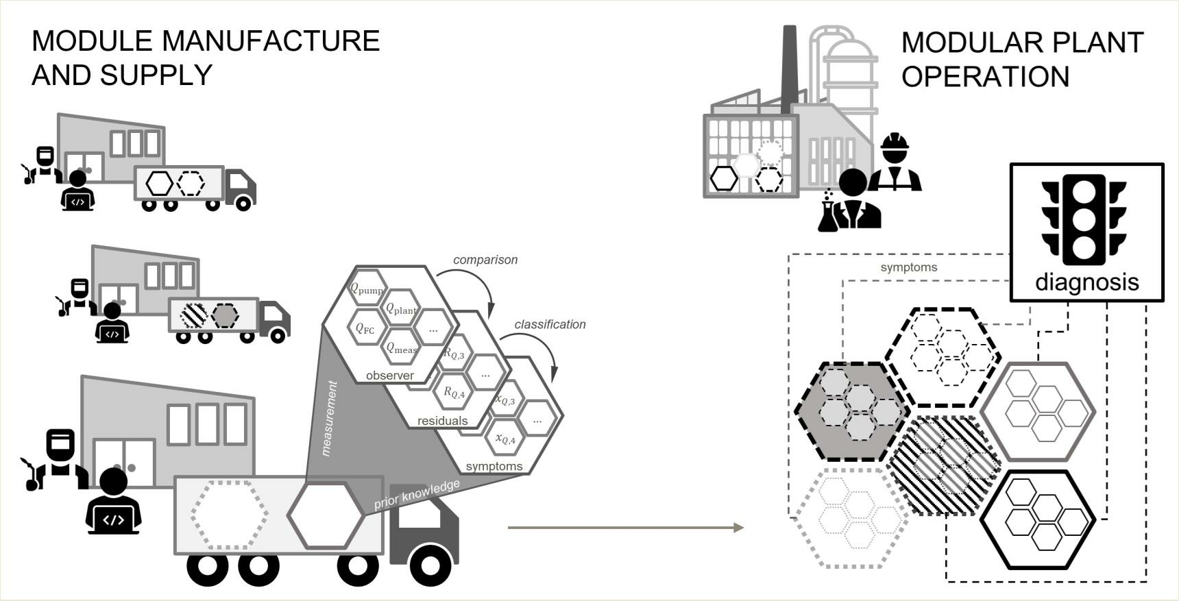
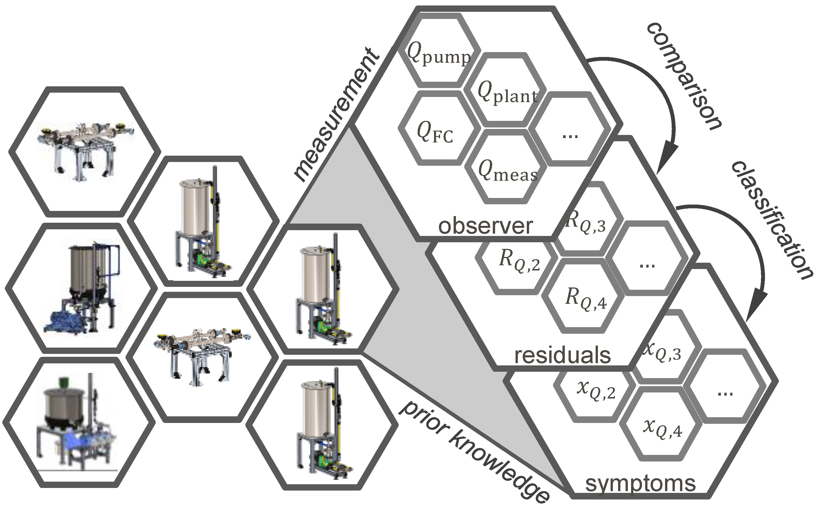
Therefore, a model-based approach is suggested to generate symptoms for each module that are independent of the overall plant topology. The procedure used to generate these symptoms consists of three steps, as seen in Figure 1: (i) observers utilize the describing model equations and the measurements of the already installed sensors to calculate state variables redundantly, (ii) to detect changes in the module’s behavior due to faults or wear, redundant state variables are subtracted from each other, resulting in residuals, and (iii) the residuals are classified, taking the current operation point of the module into account to generate symptoms.
The model-based symptoms are fueled by the supplier’s knowledge and the measurements of a few, already installed, sensors. The calculations necessary for generating the symptoms are simple and can be executed on the module’s controller. The symptoms from each module are then communicated to the central process control. This can be carried out via the manufacturer-independent interface Module-Type Package (MTP) that was specifically developed for modular process plants.
3.2. Diagnosis
The symptoms of each module are inputs for the central diagnosis system. The correct identification of the faulty module and the individual fault type can be difficult when utilizing only a few sensor measurements in each module. Therefore, the authors suggest also using the redundancies of the topology within a modular process plant. For example, if module A doses a medium into module B, then a volume flow estimation of the observer in module A can also be used in module B, given that no external leakage is present.
A central diagnosis system leveraged the knowledge of the interconnection of the modules to gain more information from the limited data. As the operator of a modular process plant knows its topology, the central diagnosis system is also their responsibility and can be implemented in the process control.
Experienced operating personnel know the correlations between certain symptoms and the cause. Rules can be derived from this knowledge and fundamental conservation equations, such as the continuity equation. A rule-based system that can be implemented using fuzzy logic is, therefore, the preferred approach for the central diagnosis system. The central diagnosis system has to be adapted every time the plant topology is reconfigured, as this is the whole point of modular process plants. To base this process on rules makes it easy to set up and adapt.
4. Implementation
In the previous chapter, the general approach for condition monitoring of modular process plants was described. The following chapter concentrates on the implementation of the model-based symptoms for different modules. The diagnosis will be addressed in future works.
While the approach can be applied to most modules, this paper focuses on two different types of modules, as they are also present in the test rig (see Figure 2): dosing modules, including different pump types, and mixing modules. In the following, the implementation of the observers, residuals, and symptoms is explained in more detail.
4.1. Observers
The observers use models to calculate state variables in different ways, thus creating redundant information for further analysis. In this paper, the redundant variable is the volume flow. The different observers rely solely on the available measurements of the pressure difference across the pumps , their rotational speed n, the pressure loss across the module , and the electric input power to their motors .
The first observer for the dosing modules is the pump observer. It is based on static pump models, which depend on the specific pump type. While feedback controllers for each module rely on dynamic models, the operation of the plant results in quasi-stationary operational conditions. Preliminary testing has shown that static models perform very well under these circumstances. For eccentric screw pumps, a modified version of the type-independent efficiency model for positive displacement pumps by Pelz and Schänzle [40] is used. Equation (1) demonstrates the model. The volume flow is calculated using the difference between a theoretical volume flow and the leakage flow , which is calculated using a semi-empirical approach represented by the model parameters , , , and .
There are other models for different pump types, such as membrane and centrifugal pumps, which are not discussed further here. The second observer is based on the pressure loss within the dosing module. This pressure loss is proportional to the squared volume flow with the plant model parameters and . Therefore, the so-called plant observer consists of the following equation:
The last observer for the dosing modules is based on the energy conservation in the module. The electric motor of the pump converts electricity into mechanical power . The pump itself uses mechanical power to increase the hydraulic power of the fluid . The power conversion is prone to losses, which are represented by the motor efficiency and the pump efficiency . The efficiencies depend on the current operating point and can be modeled via an efficiency map. If the electric power is measured, it can be used for the power observer in Equation (3):
The mixing modules rely on the observers of their upstream modules. Without external leakage, the medium conveyed by the dosing modules has to flow through the following mixing modules. Hence, a pump, plant, and power observer for the mixing modules are derived through the summation of the respective upstream observers.
There is a fourth observer for the mixing modules: the resistance observer . It is similar to the plant observer and utilizes the pressure loss across the mixing modules , which is measured through a pressure sensor. This pressure loss is again proportional to the squared volume flow and allows the estimation of the volume flow with the resistance model parameters and and the given equation:
4.2. Residual Generation
The residuals R provide information about the state of the respective modules by comparing the results of the different observers. All observers should estimate the same volume flow for normal operation. If there is a change in the system, some observers can recognize this change, whereas others cannot. This discrepancy will be obvious in the residuals, which are defined as the following subtractions for the dosing modules:
The mixing modules provide four different observers, but only the resistance observer is independent of the upstream modules. Therefore, all the residuals of the mixing modules are defined as the difference between the upstream observer and the resistance observer: .
Specific residuals will rise or fall for different types of wear or faults. In this way, they can provide valuable information for further analysis and wear detection. However, the residuals output absolute values, which are dependent on the operating point. A small residual can mean severe wear if the rotational speed of the pump is low, or negligible wear if the rotational speed is high. This ambiguity is taken into account by the classification.
4.3. Classification
The aim of the classification is to generate symptoms that are independent of the operation point and, therefore, provide unambiguous information about the module’s condition. This is implemented by linking the manufacturer’s knowledge about the residuals R at different operating points to a given condition that is represented by a symptom x. For the dosing modules, the decline in the volumetric efficiency is chosen as the symptom. The symptom x is, therefore, the difference between the volumetric efficiency of a reference module and the actual volumetric efficiency at a given reference point:
The information about the residuals at different operating points of a given module condition x is represented by 3D surfaces in the -space. These surfaces are described using polynomials. The classification works as follows: (i) measurements at the module provide information about the calculated residuals and the measured operating points ; (ii) the residuals are calculated using the polynomials; and (iii) the classification is performed by finding the closest residuals to and interpolating the symptoms x.
5. Validation
The following section describes the experimental validation of the proposed approach. The focus is on the observers, residuals, and symptoms. For this reason, the test rig used is outlined first. The validation scenarios are defined in the subsequent subsection, and finally, the results are presented.
5.1. Test Rig: Modular Mixing Plant
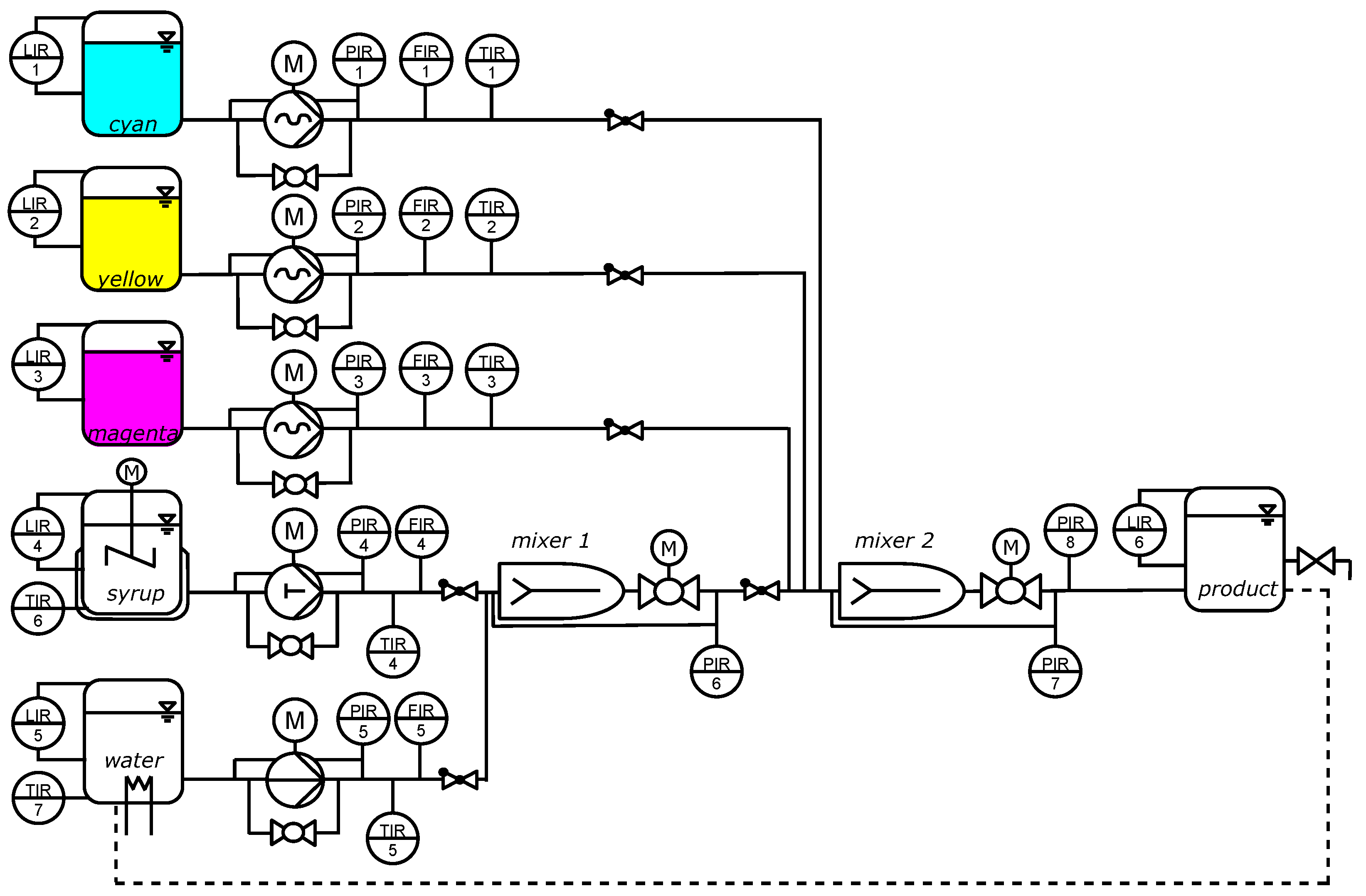
The test rig is a modular mixing plant that consists of five dosing modules and two mixing modules. A simplified piping and instrumentation diagram of the test rig is shown in Figure 2. The mixing plant is designed to produce colored sugar syrup. Therefore, the first three dosing modules are identical and dose the colors cyan, yellow, and magenta through eccentric screw pumps. The syrup dosing module is similar, but the tank has a stirrer to homogenize the syrup and contains a membrane pump. The water dosing module utilizes a centrifugal pump, and water in the tank can be heated for cleaning purposes.
Each dosing module is equipped with level and temperature sensors for its safe operation. Furthermore, the pressure difference and volume flow are measured. The electric power of the motor and its rotational speed are derived from the frequency converters that feed the electric motors. A full list of the measuring equipment used is shown in Table 1.
Each pump is additionally equipped with a bypass from the pressure to the suction side. A ball valve with a step motor usually closes the bypass in normal operation. When the ball valve is opened, the fluid will partly flow back to the suction side. This replicates an internal leakage caused by pump wear.
Mixing module 1 is fed from the syrup and water dosing modules. It consists of a static mixer and piping. Unidirectional flow is ensured by recoil check valves in the feeding pipes. The pressure difference across the mixer is detected by a differential pressure transmitter. To simulate mixer clogging, a motorized ball valve is built in series with the mixer. It is open in normal operation. Closing the ball valve increases the pressure loss across the module and decreases the flow.
Mixing module 2 is analog to mixing module 1. It is additionally fed from the three color dosing modules. The absolute pressure is measured after mixing module 2 to calculate the pressure loss between the dosing modules and the mixing modules.
5.2. Scenarios
The validation scenarios work as follows: All dosing modules operate simultaneously with different pump speeds. At first, the plant is in normal operation, i.e., all bypasses are closed and the mixer ball valves are open. The measurements of the volume flow meters are used to validate the different observers.
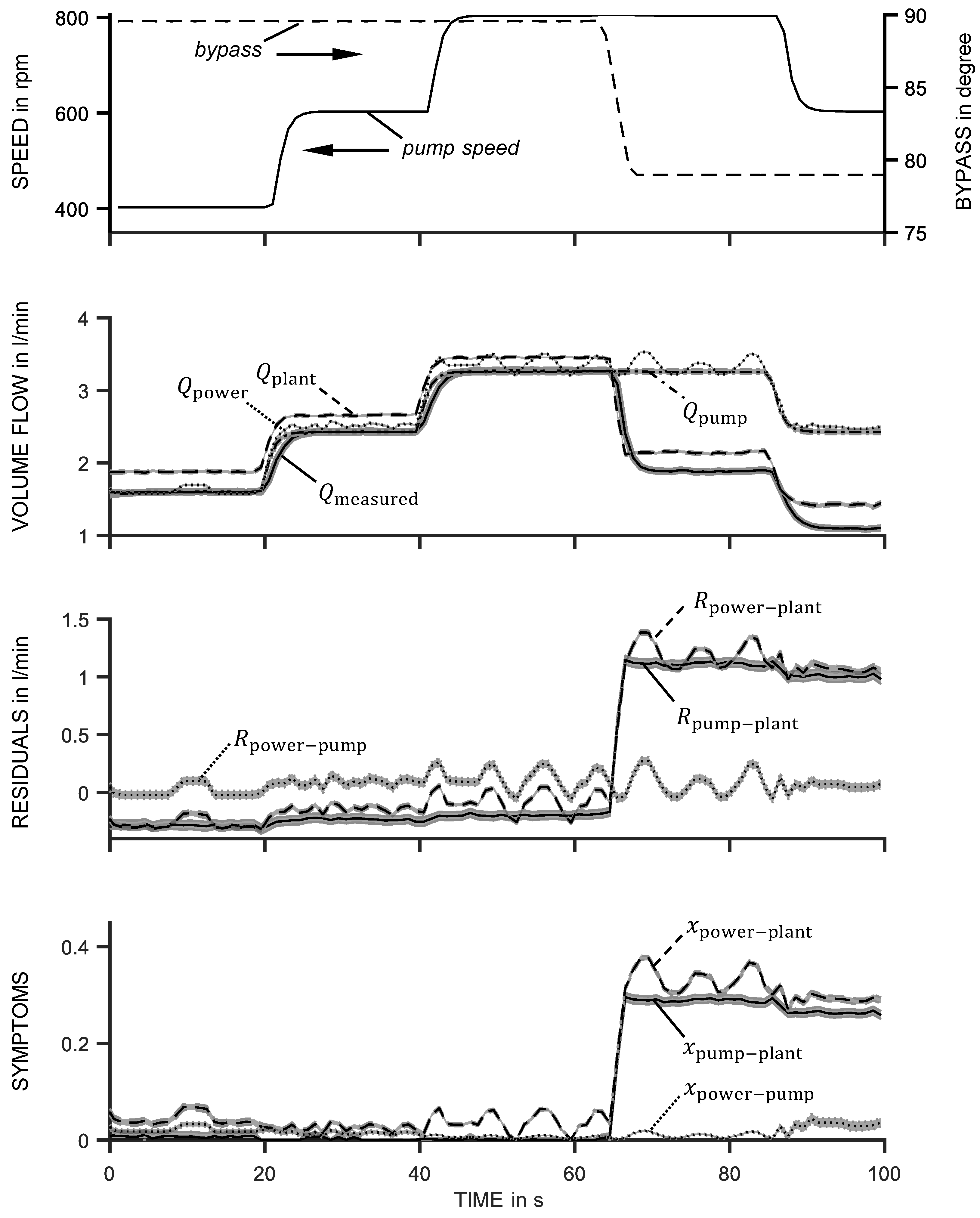
For the scenario in Figure 3, wear is introduced into the plant by opening the bypass valve of the yellow dosing module. The bypass flow reduces the volumetric efficiency of the module that is to be detected by the observers, residuals, and symptoms. For the scenario in Figure 4, the mixer is clogged by closing the mixer valve. This is carried out in two steps, resulting in different severely clogged states. All other modules remain in normal operation mode.
5.3. Uncertainty Quantification
The measurements that are conducted at the test rig are subject to uncertainty. To assess the influence of the uncertainty on the validation, it has to be quantified [41]. The systematic uncertainty of the different measurement equipment is displayed in Table 1. All sensors are operated with a sampling rate of . The calculated values for the observers, residuals, and symptoms are only of interest on a larger timescale. Therefore, temporal averaging of the measured values is applied with a resolution of . The statistical and systematic uncertainties are combined using the case of uncorrelated input quantities, cf. the Guide to the Expression of Uncertainty in Measurement (GUM) [42]. Furthermore, uncertainty propagation is conducted accordingly. The diagrams of all results contain the mean values as a line and the uncertainty as a gray interval behind the lines.
5.4. Results
The results of the validation scenarios are illustrated in Figure 3 and Figure 4. The observers in Figure 3 follow the measured volume flow quite well, as long as there is no wear. The plant observer overestimates the volume flow permanently. Starting at , the bypass valve is opened, which has a noticeable effect on the pump behavior, i.e., the volume flow decreases significantly. This is also reflected in the plant observer . The observers and do not detect the changed behavior. These observers are centered on the pump itself. The bypass flow only decreases the volume flow that leaves the module. The flow within the pump is still the same and is detected by these two observers.
This is utilized by the residuals. As seen in the third subplot in Figure 3, all residuals are close to zero in normal pump operation. The residuals and are negative due to the overestimation of the plant observer. As the bypass flow is introduced at , they increase significantly. They indicate the discrepancy between the volume flow that exits the module () and the volume flow that should be conveyed by the pump ( or ). The residual is almost zero and indicates no change, as it is based on two observers that only “see” the internal flow of the pump.
The simulated wear is constant from on. Nevertheless, the residuals decrease at when the rotational speed of the pump is reduced. This showcases the fundamental problem with absolute values. The classification is supposed to mitigate the influence of the operation point and its results are depicted in the lower subplot in Figure 3.
The negative values of and in normal operation are counteracted, resulting in a symptom that is nearly zero, indicating no wear. Once the significant wear is introduced, the symptoms and rise to values of ≈0.3 each. This represents the correct condition of the module. The change in the operation point at has a far lower impact on the symptom than on the residual. The condition is therefore presented in a more universally usable way. The combination of the two symptoms and , indicating wear, and , indicating no wear, can be interpreted by an expert or the central diagnosis system to identify the cause.
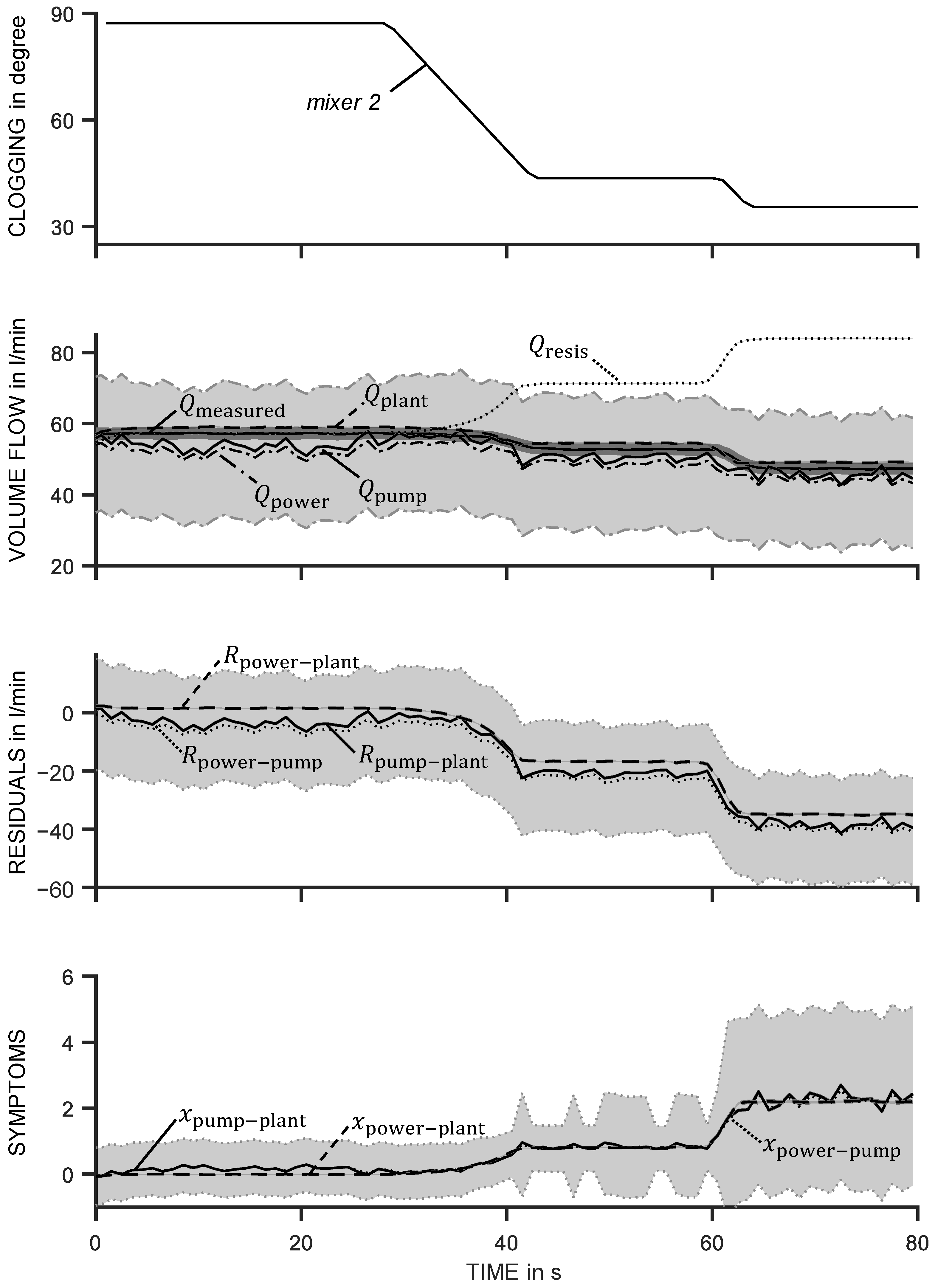
The second scenario shows the effect of mixer clogging on the observers, residuals, and symptoms. Figure 4 presents the results for the advancing wear of mixer 2. Initially, all modules operate normally. The clogging starts at and reaches a first plateau at . At , the clogging becomes more severe to reach the final mixer condition. The results for the different observers are detailed in the second subplot. The plant observer slightly overestimates the measured volume flow throughout the scenario. The pump observer and the power observer underestimate the measured values and fluctuate throughout the scenario. However, these observers are not deceived by the advancing clogging. The resistance observer estimates the real volume flow very well when there is no wear. As the observer is based on the unworn mixer behavior, it estimates an increasing volume flow due to the rising pressure loss across the clogged mixer. The difference between the estimated and the real volume flow is also reflected in the residuals. They are based on a comparison of the volume flow estimation of the preceding modules (, , ) and the estimation at the mixer itself (), and they decrease with every increase in the clogging of the mixer. The corresponding symptom is the relative variable that represents the increased pressure loss across the module and is defined as . The clogging of the mixer leads to a pressure loss of two times the original value. The power observer and its related residuals and symptoms show a higher uncertainty, which is indicated by the gray background in Figure 4. This is because it is based on uncertain efficiency maps, which are propagated through the calculations.
6. Discussion
The presented approach for condition monitoring of modular process plants is based on the separation of the symptoms per module and the central diagnosis system. The validation in this paper focuses on the first step.
The presented results show that the observers based on the manufacturer’s knowledge of individual modules work very well to estimate the volume flow for fault-free operation. Once wear is introduced to the system, the observers react in different ways, which is helpful for the residual generation. Residuals that are not zero are a strong indicator of wear in the system. To identify the magnitude of this wear, the classification is necessary and leads to symptoms that depict the effect of the wear on a module’s function.
The model-based approach for the individual modules is successful and shows how effective simple models and a few measurements can be. The efforts required for modeling are manageable, as only smaller units of the whole plant are modeled. These models are valid no matter how much the topology of the entire modular process plant is modified.
Different symptoms react to specific faults. The connections between the symptoms and their causes were not further discussed in this paper. Generally, they can be derived from expert knowledge of the modules’ interactions and the implementation of rule-based expert systems such as fuzzy inference systems, which are the subject of current research by the authors of this paper.
This overall approach offers one possibility for closing the research gap that exists for condition monitoring of modular process plants.
7. Summary and Outlook
This paper presented the concept of modular process plants to meet the demands for more flexibility and efficient production. Pre-manufactured and unvarying modules are arranged to form different plants, depending on the current recipe. To allow safe and reliable production, the plant’s condition has to be monitored. The available condition-monitoring solutions do not consider the specific challenges of modular process plants. Therefore, an approach designed specifically for modular process plants was suggested. Each module consists of several model-based observers to redundantly estimate a state variable, i.e., the volume flow. The residuals are generated by subtracting the observer outputs and hinting at changes in the system. By combining the manufacturer’s knowledge of the residuals at different operating points in given conditions, the residuals are classified and the symptoms are generated. The validation of the approach proves its feasibility, as the observer estimates the volume flow correctly in normal operation and specific residuals and symptoms increase, depending on the fault type.
So far, the last step of this approach has not been demonstrated. Based on the symptoms in each module and the expert’s/operator’s knowledge of the interactions between the modules, a central diagnosis system will be set up. By employing fuzzy logic, the symptoms will be classified, and rules based on the operator’s knowledge will be applied to receive an output for the diagnosis system. This is still the subject of current research and will be published in the next paper.
Author Contributions
Conceptualization, P.W. and P.F.P.; methodology, P.W. and P.F.P.; software, P.W.; validation, P.W.; formal analysis, P.W.; investigation, P.W.; resources, P.F.P.; data curation, P.W.; writing—original draft preparation, P.W.; writing—review and editing, P.W. and M.M.G.K.; visualization, P.W.; supervision, M.M.G.K. and P.F.P.; project administration, P.F.P.; funding acquisition, P.F.P. All authors have read and agreed to the published version of the manuscript.
Funding
This work was funded by the German Federal Ministry for Economic Affairs and Climate Action (BMWK) within the scope of the HECTOR research project as part of the ENPRO 2.0 Initiative (funding code: 03EN2006A). We acknowledge the support of the Deutsche Forschungsgemeinschaft (DFG—German Research Foundation) and the Open Access Publishing Fund of the Technical University of Darmstadt.
Data Availability Statement
The data presented in this study are available on request from the corresponding author. The data are not publicly available due to privacy concerns.
Conflicts of Interest
The authors declare no conflict of interest.
Nomenclature
The following variables are used in this manuscript:
| Pressure difference | |
| Efficiency | |
| Pump model parameter | |
| Resistance model parameter | |
| Plant model parameter | |
| n | Rotational speed |
| Electric power | |
| Q | Volume flow |
| R | Residual |
| x | Symptom |
References
- NAMUR; ProcessNet; ZVEI VDMA. Process INDUSTRIE 4.0: The Age of Modular Production on the Doorstep to Market Launch; ZVEI—German Electrical and Electronic Manufacturers’ Association: Frankfurt, Germany, 2019. [Google Scholar]
- Food and Drug Administration. Guidance for Industry: PAT—A Framework for Innovative Pharmaceutical Development, Manufacturing, and Quality Assurance; Food and Drug Administration: Rockville, MD, USA, 2004. [Google Scholar]
- Buchholz, S. F3 FACTORY (Flexible, Fast and Future Production Processes): Final Report Summary; BAYER Technology Services GmbH: Leverkusen, Germany, 2014. [Google Scholar]
- Garcia, V.; Cabassud, M.; Le Lann, M.V.; Pibouleau, L.; Casamatta, G. Constrained optimization for fine chemical productions in batch reactors. Chem. Eng. J. Biochem. Eng. J. 1995, 59, 229–241. [Google Scholar] [CrossRef]
- Martin, B.; Lehmann, H.; Yang, H.; Chen, L.; Tian, X.; Polenk, J.; Schenkel, B. Continuous manufacturing as an enabling tool with green credentials in early-phase pharmaceutical chemistry. Curr. Opin. Green Sustain. Chem. 2018, 11, 27–33. [Google Scholar] [CrossRef]
- Temporärer ProcessNet-Arbeitskreis “Modulare Anlagen”. Modular Plants: Flexible Chemical Production by Modularization and Standardization—Status Quo and Future Trends; DECHEMA e.V.: Frankfurt, Germany, 2016. [Google Scholar]
- VDI. Process Engineering Plants Modular Plants: Fundamentals and Planning Modular Plants; Beuth Verlag: Berlin, Germany, 2020. [Google Scholar]
- VDI/VDE/NAMUR. Automation Engineering of Modular Systems in the Process Industry: General Concept and Interfaces; Beuth Verlag: Berlin, Germany, 2019. [Google Scholar]
- Klose, A.; Merkelbach, S.; Menschner, A.; Hensel, S.; Heinze, S.; Bittorf, L.; Kockmann, N.; Schäfer, C.; Szmais, S.; Eckert, M.; et al. Orchestration Requirements for Modular Process Plants in Chemical and Pharmaceutical Industries. Chem. Eng. Technol. 2019, 42, 2282–2291. [Google Scholar] [CrossRef]
- Markaj, A.; Reiche, L.T.; Neuendorf, L.; Oeing, J.; Klose, A. Modularisierung in der Prozessindustrie—Bericht von der ACHEMA 2022. Chem. Ing. Tech. 2023, 95, 833–841. [Google Scholar] [CrossRef]
- Baldea, M.; Edgar, T.F.; Stanley, B.L.; Kiss, A.A. Modular manufacturing processes: Status, challenges, and opportunities. AIChE J. 2017, 63, 4262–4272. [Google Scholar] [CrossRef]
- Sharif, M.A.; Grosvenor, R.I. Process plant condition monitoring and fault diagnosis. Proc. Inst. Mech. Eng. Part E J. Process. Mech. Eng. 1998, 212, 13–30. [Google Scholar] [CrossRef]
- Bagavathiappan, S.; Lahiri, B.B.; Saravanan, T.; Philip, J.; Jayakumar, T. Infrared thermography for condition monitoring—A review. Infrared Phys. Technol. 2013, 60, 35–55. [Google Scholar] [CrossRef]
- Toms, A.; Toms, L. Oil Analysis and Condition Monitoring. In Chemistry and Technology of Lubricants; Mortier, R.M., Fox, M.F., Orszulik, S.T., Eds.; Springer: Dordrecht, The Netherlands, 2010; pp. 459–495. [Google Scholar] [CrossRef]
- Al-Obaidi, S.M.A.; Leong, M.S.; Hamzah, R.R.; Abdelrhman, A.M. A Review of Acoustic Emission Technique for Machinery Condition Monitoring: Defects Detection & Diagnostic. Appl. Mech. Mater. 2012, 229–231, 1476–1480. [Google Scholar] [CrossRef]
- Buchanan, B.G.; Smith, R.G. Fundamentals of Expert Systems. Annu. Rev. Comput. Sci. 1988, 3, 23–58. [Google Scholar] [CrossRef]
- Ebersbach, S.; Peng, Z. Expert system development for vibration analysis in machine condition monitoring. Expert Syst. Appl. 2008, 34, 291–299. [Google Scholar] [CrossRef]
- Casal-Guisande, M.; Comesaña-Campos, A.; Pereira, A.; Bouza-Rodríguez, J.B.; Cerqueiro-Pequeño, J. A Decision-Making Methodology Based on Expert Systems Applied to Machining Tools Condition Monitoring. Mathematics 2022, 10, 520. [Google Scholar] [CrossRef]
- Žarković, M.; Stojković, Z. Analysis of artificial intelligence expert systems for power transformer condition monitoring and diagnostics. Electr. Power Syst. Res. 2017, 149, 125–136. [Google Scholar] [CrossRef]
- Isermann, R. Fault-Diagnosis Applications: Model-Based Condition Monitoring: Actuators, Drives, Machinery, Plants, Sensors, and Fault-Tolerant Systems; Springer: Berlin/Heidelberg, Germany, 2011. [Google Scholar]
- Isermann, R. Fault-Diagnosis Systems: An Introduction from Fault Detection to Fault Tolerance; Springer: Berlin/Heidelberg, Germany, 2006. [Google Scholar]
- Lyubenova, V.; Kostov, G.; Denkova-Kostova, R. Model-Based Monitoring of Biotechnological Processes—A Review. Processes 2021, 9, 908. [Google Scholar] [CrossRef]
- Chen, G.Q. New challenges and opportunities for industrial biotechnology. Microb. Cell Factories 2012, 11, 111. [Google Scholar] [CrossRef]
- Misawa, E.A.; Hedrick, J.K. Nonlinear Observers—A State-of-the-Art Survey. J. Dyn. Syst. Meas. Control 1989, 111, 344–352. [Google Scholar] [CrossRef]
- Reif, K.; Unbehauen, R. The extended Kalman filter as an exponential observer for nonlinear systems. IEEE Trans. Signal Process. 1999, 47, 2324–2328. [Google Scholar] [CrossRef]
- Bastin, G.; Dochain, D. On-Line Estimation and Adaptive Control of Bioreactors; Volume 1, Process Measurement and Control; Elsevier: Amsterdam, The Netherlands, 1990. [Google Scholar]
- Cross, P.; Ma, X. Model-based and fuzzy logic approaches to condition monitoring of operational wind turbines. Int. J. Autom. Comput. 2015, 12, 25–34. [Google Scholar] [CrossRef]
- Charles, G.; Goodall, R.; Dixon, R. Model-based condition monitoring at the wheel–rail interface. Veh. Syst. Dyn. 2008, 46, 415–430. [Google Scholar] [CrossRef]
- Shi, H.T.; Bai, X.T. Model-based uneven loading condition monitoring of full ceramic ball bearings in starved lubrication. Mech. Syst. Signal Process. 2020, 139, 106583. [Google Scholar] [CrossRef]
- Patton, R.J.; Chen, J.; Nielsen, S.B. Model-based methods for fault diagnosis: Some guide-lines. Trans. Inst. Meas. Control 1995, 17, 73–83. [Google Scholar] [CrossRef]
- Althubaiti, A.; Elasha, F.; Teixeira, J.A. Fault diagnosis and health management of bearings in rotating equipment based on vibration analysis—A review. J. Vibroeng. 2022, 24, 46–74. [Google Scholar] [CrossRef]
- KSB Limited. KSB Guard Homepage. Available online: https://www.ksb.com/en-gb/lc/products/pump-automation/ksb-guard/G01A (accessed on 24 May 2023).
- Sulzer. Sulzer Sense Condition Monitoring Solution: Let Sense Take Care of Your Pump 24/7. Available online: https://www.sulzer.com/en/shared/products/sulzer-sense-condition-monitoring (accessed on 24 May 2023).
- DYNAPAR. Dynapar OnSite™ Online Condition Monitoring System. Available online: https://www.dynapar.com/products_and_solutions/condition_monitoring/ (accessed on 24 May 2023).
- Goyal, D.; Pabla, B.S. The Vibration Monitoring Methods and Signal Processing Techniques for Structural Health Monitoring: A Review. Arch. Comput. Methods Eng. 2016, 23, 585–594. [Google Scholar] [CrossRef]
- Qiu, S.; Cui, X.; Ping, Z.; Shan, N.; Li, Z.; Bao, X.; Xu, X. Deep Learning Techniques in Intelligent Fault Diagnosis and Prognosis for Industrial Systems: A Review. Sensors 2023, 23, 1305. [Google Scholar] [CrossRef] [PubMed]
- Kalmár, C.; Hegedűs, F. Condition Monitoring of Centrifugal Pumps Based on Pressure Measurements. Period. Polytech. Mech. Eng. 2019, 63, 80–90. [Google Scholar] [CrossRef]
- Surek, D. Pumpen für Abwasser- und Kläranlagen: Auslegung und Praxisbeispiele; Springer Fachmedien Wiesbaden: Wiesbaden, Germany, 2014. [Google Scholar]
- Kudelina, K.; Vaimann, T.; Asad, B.; Rassõlkin, A.; Kallaste, A.; Demidova, G. Trends and Challenges in Intelligent Condition Monitoring of Electrical Machines Using Machine Learning. Appl. Sci. 2021, 11, 2761. [Google Scholar] [CrossRef]
- Schänzle, C.; Jost, K.; Lemmer, J.; Metzger, M.; Ludwig, G.; Pelz, P.F. ERP Positive Displacement Pumps—Experimental Validation of a Type-Independent Efficiency Model. In Proceedings of the 4rd International Rotating Equipment Conference, Wiesbaden, Germany, 23–24 September 2019. [Google Scholar]
- Pelz, P.F.; Groche, P.; Pfetsch, M.E.; Schaeffner, M. Mastering Uncertainty in Mechanical Engineering; Springer International Publishing: Cham, Switzerland, 2021. [Google Scholar] [CrossRef]
- Joint Committee for Guides in Metrology. Evaluation of Measurement Data—Guide to the Expression of Uncertainty in Measurement; Bureau International des Poids et Mesures: Sèvres Cedex, France, 2008. [Google Scholar]
Figure 1.
Approach for the model-based symptoms of each module.

Figure 2.
Piping and instrumentation diagram of modular mixing plant.

Figure 3.
Results for the speed-up of the color dosing module: at the pump condition noticeably changes.
Figure 3.
Results for the speed-up of the color dosing module: at the pump condition noticeably changes.

Figure 4.
Results for the clogging of mixing module 2: the uncertainty intervals of , , and are indicated by the gray background.
Figure 4.
Results for the clogging of mixing module 2: the uncertainty intervals of , , and are indicated by the gray background.


Table 1.
Sensors on the test rig.
| Variable | Sensor Type | Systematic Uncertainty |
|---|---|---|
| piezoresistive pressure transmitter | ||
| n | frequency converter | |
| Q | magnetic-inductive flow meters | |
| frequency converter | ||
| l | ultrasonic level sensor | |
| T | resistance thermometer |
Disclaimer/Publisher’s Note: The statements, opinions and data contained in all publications are solely those of the individual author(s) and contributor(s) and not of MDPI and/or the editor(s). MDPI and/or the editor(s) disclaim responsibility for any injury to people or property resulting from any ideas, methods, instructions or products referred to in the content. |
© 2023 by the authors. Licensee MDPI, Basel, Switzerland. This article is an open access article distributed under the terms and conditions of the Creative Commons Attribution (CC BY) license (https://creativecommons.org/licenses/by/4.0/).
Share and Cite
MDPI and ACS Style
Wetterich, P.; Kuhr, M.M.G.; Pelz, P.F. Model-Based Condition Monitoring of Modular Process Plants. Processes 2023, 11, 2733. https://doi.org/10.3390/pr11092733
AMA Style
Wetterich P, Kuhr MMG, Pelz PF. Model-Based Condition Monitoring of Modular Process Plants. Processes. 2023; 11(9):2733. https://doi.org/10.3390/pr11092733
Chicago/Turabian StyleWetterich, Philipp, Maximilian M. G. Kuhr, and Peter F. Pelz. 2023. "Model-Based Condition Monitoring of Modular Process Plants" Processes 11, no. 9: 2733. https://doi.org/10.3390/pr11092733
Note that from the first issue of 2016, this journal uses article numbers instead of page numbers. See further details here.