
Explainable Machine Learning-Based Method for Fracturing Prediction of Horizontal Shale Oil Wells
 , , ,
, , ,
Abstract
:1. Introduction
2. Methodology
2.1. GBDT (Gradient Boosting Decision Tree)
2.2. PSO (Particle Swarm Optimization)
2.3. Machine Learning Model Interpretability
2.3.1. LIME (Local Interpretable Model-Agnostic Explanations)
2.3.2. SHAP (Shapley Additive Explainable)
3. Workflow
4. Results and Discussion
4.1. Work Zone Overview
4.2. Data Analysis
4.2.1. Data Collection and Analysis
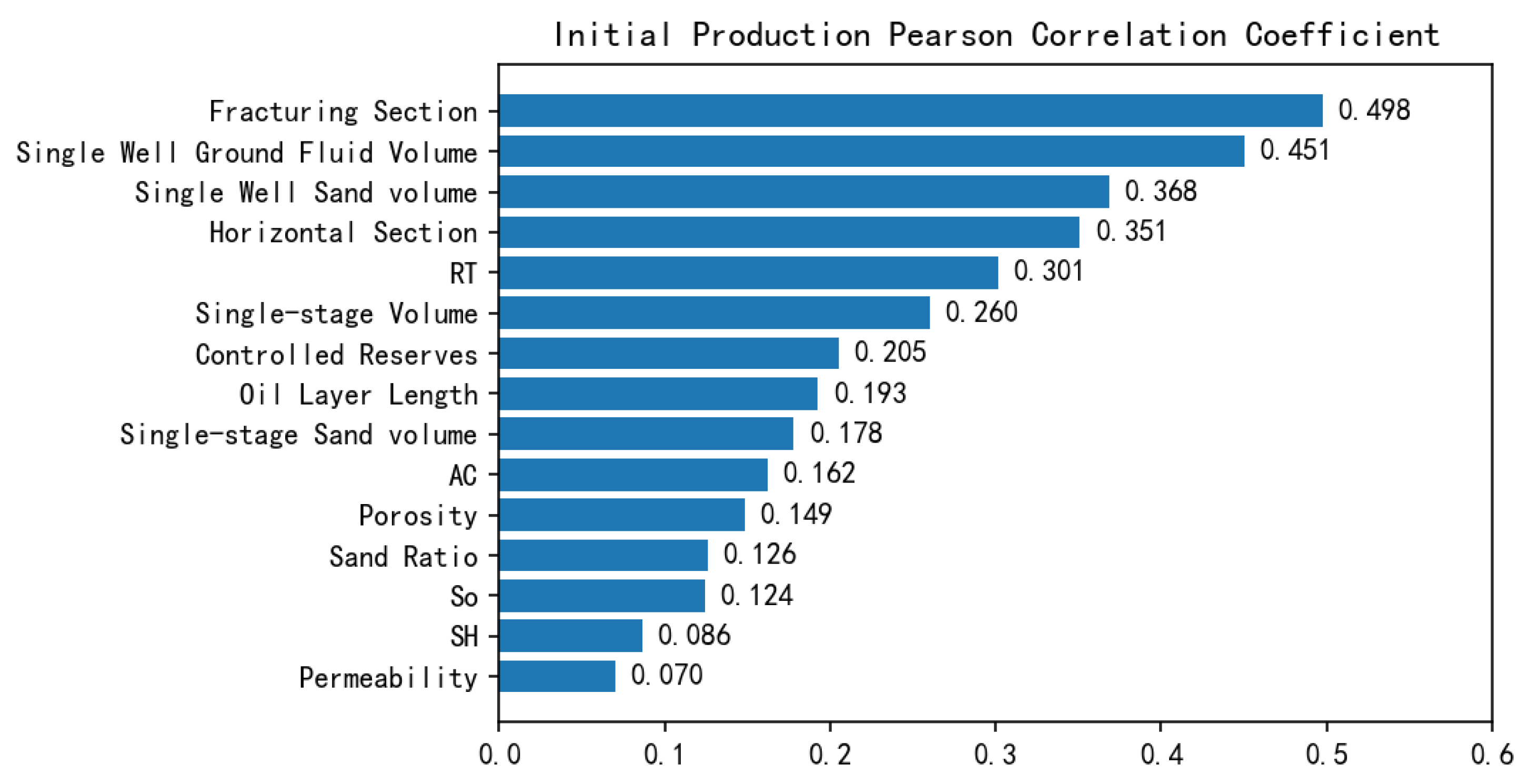
4.2.2. Correlation Analysis
4.3. Machine Learning Model Building
4.4. Explanation of the Forecasting Model
4.4.1. Local Explanation
- (1)
- LIME
- (2)
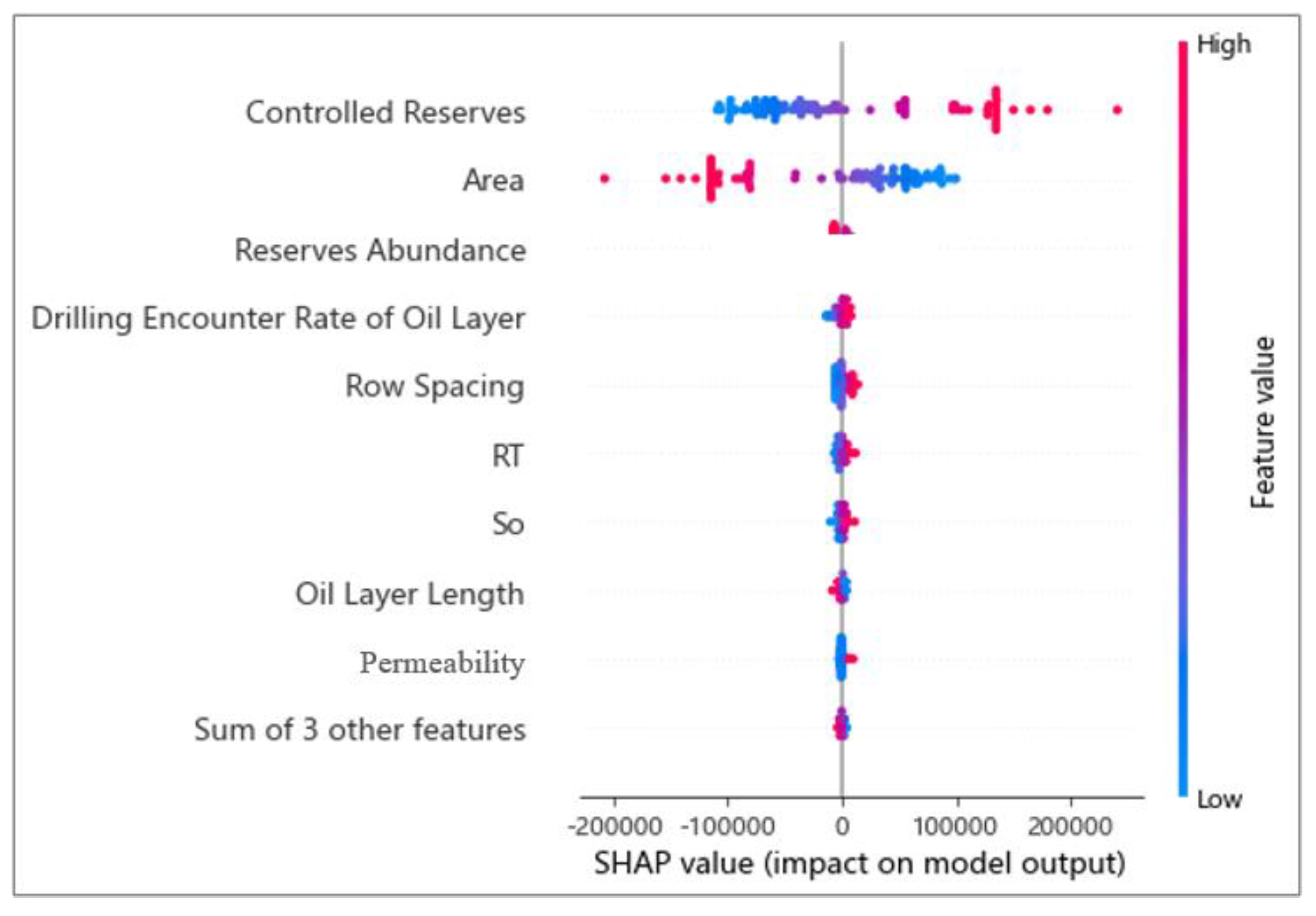
- SHAP
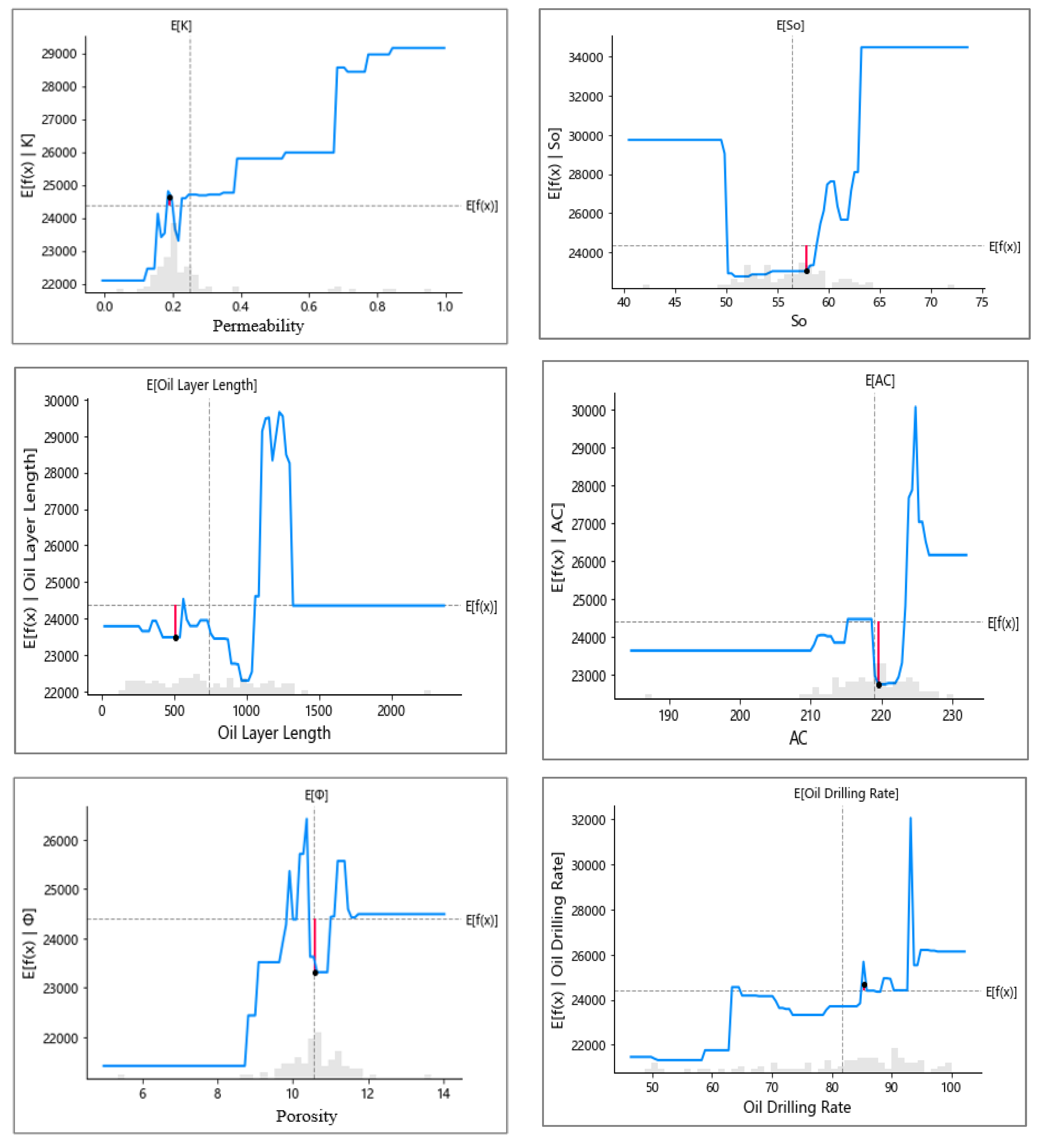
4.4.2. Global Analysis
5. Discussion and Conclusions
5.1. Discussion
5.2. Conclusions
Author Contributions
Funding
Data Availability Statement
Acknowledgments
Conflicts of Interest
References
- Hu, S.; Zhap, W.; Hou, L.; Yang, Z.; Zhu, R.; Wu, S.; Bai, B.; Jin, X. Development potential and technical strategy of continental shale oil in China. Pet. Explor. Dev. 2020, 47, 819–828. [Google Scholar] [CrossRef]
- Lu, Y. Advances and Applications of Fracturing Technology in Shale Reservoirs; Petroleum Industry Press: Beijing, China, 2016. [Google Scholar]
- Li, Z.; Li, F.; Huang, Z. The key role of hydraulic fracturing in oil and gas field exploration and development. Oil Gas Geol. Recovery 2010, 17, 76–79+116. [Google Scholar]
- Liang, Z. Dense cutting and multi-cluster volume fracturing technology for horizontal wells in well block 30 of Dongsheng gas field. Pet. Geol. Eng. 2022, 36, 98–101+108. [Google Scholar]
- Ling, T. Study on Optimization of Horizontal Well Fracturing in Shale Oil; Northeastern Petroleum University: Daqing, China, 2022. [Google Scholar]
- Kuangsheng, Z.H.A.N.G.; Meirong, T.A.N.G.; Liang, T.A.O.; Xianfei, D.U. Horizontal well volumetric fracturing technology integrating fracturing, energy enhancement, and imbibition for shale oil in Qingcheng Oilfield. Pet. Drill. Tech. 2022, 50, 9–15. [Google Scholar]
- Zou, C.; Pan, S.; Jing, Z.; Gao, J.; Yang, Z.; Wu, S.; Zhao, Q. Shale oil and gas revolution and its impact. Acta Pet. Sin. 2020, 41, 1–12. [Google Scholar]
- Jiang, T.; Wang, B.; Shan, W.; Li, A. A theoretical model for overall fracturing optimization scheme design. J. Pet. 2001, 5, 58–62+2. [Google Scholar]
- Fan, Y.; Ma, X.; Lian, J. Research and comparison of filling methods for missing data in hydraulic fracturing. Petrochem. Ind. Appl. 2020, 39, 48–55. [Google Scholar]
- Wang, H.; Mu, L.; Shi, F.; Dou, H. Production prediction at ultra-high water cut stage via Recurrent Neural Network. Pet. Explor. Dev. 2020, 47, 1009–1015. [Google Scholar] [CrossRef]
- Costa, L.; Maschio, C.; Schiozer, D. Application of artificial neural networks in a history matching process. J. Pet. Sci. Eng. 2014, 123, 30–45. [Google Scholar] [CrossRef]
- Luo, G.; Tian, Y.; Bychina, M.; Ehlig-Economides, C. Production-Strategy Insights Using Machine Learning: Application for Bakken Shale. SPE Reserv. Eval. Eng. 2019, 22, 800–816. [Google Scholar] [CrossRef]
- Liang, Y.; Zhao, P. A Machine Learning Analysis Based on Big Data for Eagle Ford Shale Formation. In Proceedings of the SPE Annual Technical Conference and Exhibition, Calgary, AB, Canada, 30 September–2 October 2019. [Google Scholar]
- Esmaili, S.; Mohaghegh, S.D. Full field reservoir modeling of shale assets using advanced data-driven analytics. Geosci. Front. 2016, 7, 11–20. [Google Scholar] [CrossRef]
- Duplyakov, V.; Morozov, A.; Popkov, D.; Vainshtein, A.; Osiptsov, A.; Burnaev, E.; Shel, E.; Paderin, G.; Kabanova, P.; Fayzullin, I.; et al. Practical Aspects of Hydraulic Fracturing Design Optimization using Machine Learning on Field Data: Digital Database, Algorithms and Planning the Field Tests. In Proceedings of the SPE Symposium: Hydraulic Fracturing in Russia, Experience and Prospects, Virtual, 22 September 2020. [Google Scholar]
- Wu, H. Research on the Optimization Model of Shale Gas Well Fracturing Based on Machine Learning; China University of Petroleum: Beijing, China, 2020. [Google Scholar] [CrossRef]
- Li, J.; Chen, C.; Xiao, J. Yield prediction of shale gas muti-stage fracturing wells based on random forest algorithm. J. Yangtze Univ. (Nat. Sci. Ed.) 2020, 17, 34–38. [Google Scholar]
- Yan, Z.; Wang, T.; Liu, Z.; Zhuang, Z. Machine-learning-based Prediction Methods on Shale Gas Recovery. CHINese J. Solid Mech. 2021, 42, 221–232. [Google Scholar] [CrossRef]
- Ma, X.; Fan, Y. Productivity prediction model for vertical fractured well based on machine learning. Math. Pract. Theory 2021, 51, 186–196. [Google Scholar]
- Kubota, L.K.; Reinert, D. Machine learning forecasts oil rate in mature onshore field jointly driven by water and steam injection. In Proceedings of the SPE Annual Technical Conference and Exhibition, Calgary, AB, Canada, 30 September–2 October 2019. [Google Scholar]
- Bao, A.; Gildin, E.; Huang, J.; Coutinho, E.J. Data-driven end-to-end production prediction of oil reservoirs by En KF-enhanced recurrent neural networks. In Proceedings of the SPE Latin American and Caribbean Petroleum Engineering Conference, Virtual, 27–31 July 2020. [Google Scholar]
- Perez, H.H.; Datta-Gupta, A.; Mishra, S. The Role of Electrofacies, Lithofacies, and Hydraulic Flow Units in Permeability Predictions from Well Logs: A Comparative Analysis Using Classification Trees. Soc. Pet. Eng. 2005, 8, 143–155. [Google Scholar] [CrossRef]
- Breiman, L. Random Forests. Mach. Learn. 2001, 45, 5–32. [Google Scholar] [CrossRef]
- Molnar, C. Interpretable Machine Learning [M/OL]. Available online: https://christophm.github.io/interpretable-m-book (accessed on 29 March 2022).
- Guidotti, R.; Monreale, A.; Ruggieri, S.; Turini, F.; Giannotti, F.; Pedreschi, D. Asurvey of methods for explaining black box models. ACM Comput. Surv. 2018, 51, 93–100. [Google Scholar] [CrossRef]
- Baehrens, D.; Schroeter, T.; Harmeling, S.; Kawanabe, M.; Hansen, K.; Müller, K.R. How to explain individual classification decisions. J. Mach. Learn. Res. 2010, 11, 1803–1831. [Google Scholar] [CrossRef]
- Feng, D.; Wu, G. Interpretable machine learning-based modeling approach for fundamental properties of concretcstructures. J. Build. Struct. 2022, 43, 228–238. [Google Scholar] [CrossRef]
- Mai-Cao, L.; Truong-Khac, H. A Comparative Study on Different Machine Learning Algorithms for Petroleum Production Forecasting. Improv. Oil Gas Recover 2022, 6, 1–8. [Google Scholar] [CrossRef]
- Doan, T.; Vo, M.V. Using Machine Learning Techniques for Enhancing Production Forecast in North Malay Basin. Improv. Oil Gas Recovery 2021, 5, 1–7. [Google Scholar] [CrossRef]
- Hou, Y.; Wu, Y.; Hu, X.; Tang, M.; Liu, Y.; Zhang, J.; Niu, L.; Xu, W. Fracturing and Production Observations from the First Two Horizontal Wells for Shale Oil Exploration in Ordos Basin. In Proceedings of the Abu Dhabi International Petroleum Exhibition & Conference, Abu Dhabi, United Arab Emirates, 9–12 November 2020. [Google Scholar] [CrossRef]


| Time | Author | Data | Methods | Importation | Objectives | Research Block | Accuracy |
|---|---|---|---|---|---|---|---|
| 2016 [14] | Esmaili | 3700 | Data-driven technology | Well locations, trajectories, static data, completion, hydraulic fracturing data, production rates, and operational constraints | Forecast well production | Marcellus Shale Oil and Gas, Southwestern Pennsylvania | 97.18% |
| 2019 [12] | Luo G, Tian Y | 2061 | Random Forest, Recursive Feature Elimination, Lasso Regularization Analysis | Formation pressure, porosity, reservoir thickness, TOC, thermal maturity, and brittleness | Forecast production | Bakken Shale Oil | 60.00% |
| 2020 [15] | Duplyakoz | 5500 | Hydraulic Fracturing Database | Formation parameters, well structure, field and layer IDs, all HF design parameters | Predicted production, fracturing design optimization | Data on 22 oil fields in Western Siberia, Russia | 64.80% |
| 2020 [16] | Wu Hua | 137 | RF, BP, XGBoost | Formation parameters, reservoir parameters, and fracturing parameters | Production, Fracturing parameter optimization | Weiyuan block | 79.00% |
| 2020 [17] | Li Juhua et al. | 196 | RF | Formation parameters, reservoir parameters | Predicted gas well production | Fuling Shale Gas Field | 72.30% |
| 2021 [18] | Yan Ziming | 186 | XGBoost, DNN, SVR | Formation parameters, reservoir parameters | Predicted recovery | Fuling Shale Gas Field | 85.30% |
| 2022 [19] | Ma Xianlin, Zhou Desheng, and Cai Wenbin | 598 | ANN, SVM, RF, GBDT SHAP Explanation | Formation parameters, reservoir parameters, and fracturing parameters | Horizontal well prediction, model interpretation | Surig Gas Field East | Train: 67.00% Test: 58.00% |
| Type | Parameters | |
|---|---|---|
| Input Parameters | Geological parameters | Well Distance, Row Spacing, Area, Reserves Abundance, Controlled Reserves, Oil Layer Length, Poor Oil Layer, Drilling Encounter Rate of Oil Layer, RT (Resistivity), AC (Acoustic time difference), SH (Shale volume), Φ (Porosity), K (Permeability), So (Oil saturation) |
| Engineering Parameters | Horizontal Section, Fracturing Section, Single Well Ground Fluid Volume, Single Well Sand Proportion, Single-stage Sand Volume, Sand Ratio, Single-stage Volume | |
| Output parameters | Production Dynamic Parameters | Initial Production, EUR (Estimated ultimate recovery) |
| Parameters | Distributions | ||
|---|---|---|---|
| Percentage of Wells | Spilt Point | Percentage of Wells | |
| RT | 20% | 50 Ω·m | 80% |
| Controlled Reserves | 60% | 50 × 108 m3 | 10% |
| Oil layer length | 60% | 1000 m | 60% |
| AC value | 80% | 220 | 20% |
| Porosity | 25% | 0.1 | 75% |
| So | 7% | 0.5 | 93% |
| SH | 35% | 0.15 | 65% |
| Permeability | 99% | 0.5 md | 1% |
| Area | 99.5% | 2 | 0.5% |
| Drilling encounter rate of oil layer | 35% | 80% | 65% |
| Reserves Abundance | 50% | 44 | 50% |
| Poor oil layer | 85% | 1000 | 15% |
| Parameters | Distributions | ||
|---|---|---|---|
| Percentage of Wells | Spilt Point | Percentage of Wells | |
| Fracturing section | 70% | 20 | 30% |
| Single well ground fluid volume | 60% | 20,000 m3 | 40% |
| Single well sand proportion of wells | 58% | 2000 m3 | 42% |
| Horizontal section | 90% | 2000 m | 10% |
| Single-stage volume | 48% | 10 m3/min | 52% |
| Sand ratio | 77% | 20% | 23% |
| Row spacing | 55% | 200 m | 45% |
| N_Estimators | Learning Rate | ax_Depth | Alpha | ||
|---|---|---|---|---|---|
| Default value | 100 | 0.3 | 6 | 0.9 | |
| Value ranges | 10–1000 | 0–1 | 1–100 | 0.5–0.95 | |
| Optimal values | XGB | 122 | 0.11 | 22 | 0.80 |
| Light GBM | 453 | 0.19 | 14 | 0.33 | |
| GBDT | 848 | 0.30 | 2 | 0.51 | |
Disclaimer/Publisher’s Note: The statements, opinions and data contained in all publications are solely those of the individual author(s) and contributor(s) and not of MDPI and/or the editor(s). MDPI and/or the editor(s) disclaim responsibility for any injury to people or property resulting from any ideas, methods, instructions or products referred to in the content. |
© 2023 by the authors. Licensee MDPI, Basel, Switzerland. This article is an open access article distributed under the terms and conditions of the Creative Commons Attribution (CC BY) license (https://creativecommons.org/licenses/by/4.0/).
Share and Cite
Liu, X.; Zhang, T.; Yang, H.; Qian, S.; Dong, Z.; Li, W.; Zou, L.; Liu, Z.; Wang, Z.; Zhang, T.; et al. Explainable Machine Learning-Based Method for Fracturing Prediction of Horizontal Shale Oil Wells. Processes 2023, 11, 2520. https://doi.org/10.3390/pr11092520
Liu X, Zhang T, Yang H, Qian S, Dong Z, Li W, Zou L, Liu Z, Wang Z, Zhang T, et al. Explainable Machine Learning-Based Method for Fracturing Prediction of Horizontal Shale Oil Wells. Processes. 2023; 11(9):2520. https://doi.org/10.3390/pr11092520
Chicago/Turabian StyleLiu, Xinju, Tianyang Zhang, Huanying Yang, Shihao Qian, Zhenzhen Dong, Weirong Li, Lu Zou, Zhaoxia Liu, Zhengbo Wang, Tao Zhang, and et al. 2023. "Explainable Machine Learning-Based Method for Fracturing Prediction of Horizontal Shale Oil Wells" Processes 11, no. 9: 2520. https://doi.org/10.3390/pr11092520