Intelligent Control of Thermal Energy Storage in the Manufacturing Sector for Plant-Level Grid Response

Abstract

Industrial facilities are seeking new strategies that help in providing savings mechanisms for demand charges. Demand charges are the charges incurred by industrial facilities as a result of power usage. Thermal energy storage has advanced significantly with lots of new applications, garnering the interest of many industrial facilities. These applications could be used to shave the industrial facilities’ peak electric demand and reduce their demand charges. This paper aims to demonstrate the efficacy of thermal energy storage in reducing demand charges and highlight new developments in the integration of smart control systems with thermal energy storage. The study compares energy consumption and peak demand for a facility equipped with and without thermal energy storage tanks using a fixed schedule for charging and discharging. Additionally, the paper examines the impact of incorporating a smart controller to determine when to charge and discharge the tank based on the facility’s real-time power usage and a given setpoint. The results indicate cost savings from the use of thermal energy storage tanks under two proposed scenarios, reflected in the reduced cost of power consumption for the studied facility. The incorporation of a smart controller with the thermal energy storage tank in the facility studied could provide estimated savings of 3.3% per year of power consumption charges, without considering the contribution of any incentives. The estimated savings provided by the fixed schedule scenario are 2.7% per year.

1. Introduction

Every industrial facility has an electric demand profile that represents its power usage. Manipulation of the industrial facilities’ electric demand profile has earned the interest of industry pioneers, especially in recent years due to the initiatives and new developments that help in providing various strategies and applications to reduce power demand charges. Many studies have worked on strategies to achieve power and energy savings such as that by Lee and Cheng [1] and another study about a review on energy saving strategies by Abdelaziz et al. [2]. Some researchers focused on increasing the facility’s energy efficiency such as the studies by Aflaki et al. [3] and Laitner [4]. There is a specific case in California where the aggregate demand of the entire system using electricity minus the load generated by renewable energy has a demand curve resembling the shape of a duck, and that is why it was named “The duck curve” [5]. Several researchers have conducted studies on how to manage the duck curve to achieve energy savings. For example, Krietemeyer et al. [6] published a paper in 2021 explaining a local energy management program with the potential to flatten the duck curve.

Energy assessments are critical to study the capability of facilities to achieve energy and power savings. Patterson et al. [7] focused on the current practices and recommendations of the Industrial Energy Assessments Centers (IACs) sponsored by the U.S. Department of Energy (DOE). Some energy assessments provide recommendations on how to manipulate the facility’s power profile to achieve demand charge savings. Most of these strategies involve a process called demand side management. Demand side management strategies provide saving mechanisms for industrial facilities by manipulating their demand profile [8,9,10]. One promising strategy for demand side management is energy storage, which is one of the core pillars of this study.

Energy storage has caught the attention of many researchers, especially regarding the industrial sector, owing to the potential savings provided by the various applications of energy storage. Schmalensee [11] explained how competitive energy storage is in manipulating the duck curve, while Zhang et al. [12] presented a study about the recent developments regarding thermal energy storage (TES) and Alva et al. [13] gave an overview of TES systems and their potential in providing demand charge savings. Kosowatz [14] conducted research on the energy storage contribution in smoothing the duck curve, which is similar to the study of flattening the duck curve [6]. Chen et al. [15] performed a case study on the effect of smart pumping and water storage, battery storage, and solar panels on the demand profile, similar to the objective of this paper but with different applications. Recently, new applications have combined renewable energy forms with energy storage systems. Saffari et al. [16] and Pitra et al. [17] have published papers involving studies of energy storage integrated with renewable energy, specifically solar PV. Powell and Edgar [18] presented dynamic simulation results of adding thermal energy storage with advanced control techniques to concentrating solar power. Immonen et al. [19] performed a case study about dynamic optimization with flexible heat integration of solar energy with TES for industrial process heat, while Howlader et al. [20] introduced pumped storage hydroelectricity. The high interest of the researchers in the field of thermal energy storage applications shows how promising these applications are, especially the applications of integrating thermal energy storage with renewable energy forms.

The main objective of this case study is to highlight the potential savings from the implementation of real-time demand response control strategies using TES for an industrial facility. The main addition of the paper to TES applications is having a smart controller that maintains the power usage of industrial facilities at a given setpoint using the flexible charging and discharging of TES.

The core points discussed in the paper are

• Incorporating TES with the modeling of a stratified TES tank;
• Using TES in two possible scenarios of process simulation;
• Presenting the potential savings from employing the two scenarios utilizing TES and highlighting the novelty of the paper, which is the application of the smart controller integrated with TES, which has a given setpoint to maintain the power usage of industrial facilities.

Looking at the literature of the optimization applications utilizing TES, Powell et al. [21] published a paper about the optimal loading of a system with a chiller integrated with TES. McLaughlin and Choi [22] published a paper about estimating energy savings by utilizing machine learning models in industrial energy systems. Chen et al. [23] examined the case of using intelligent control strategies with built-in storage of renewable energy, while Palensky and Dietrich [24] implemented intelligent control strategies for demand side management. Jo and Park [25] examined the strategy of demand side management with energy storage integrated with a smart grid. Powell et al. [26] tackled the topic of dynamic optimization of a campus cooling system with TES. Industrial facilities also considered stochastic optimization to be implemented with TES tanks for energy savings [27,28,29], where these three case studies explained the potential of stochastic optimization with energy storage. The difference between stochastic optimization and the application of this case study is that this case study has a controller with an optimized setpoint to control the power usage of an industrial facility. Looking at the literature and the published papers, this paper provides a new optimization method that maintains the power usage of industrial facilities at a specific setpoint to achieve optimum electric demand charge savings. Electric demand charges are the charges that any industrial facility incurs due to power consumption (Section 2.3). This paper conducts the case study using real data from a facility that uses chillers for process cooling purposes. An added TES tank will store the chilled water and provide the cooling load to the process during necessary periods. The chillers have variable-frequency drives (VFDs), which are considered manipulated variables for the smart controller to meet the process cooling needs. Two papers showed energy savings achieved by applying VFDs on compressors and motors [30,31].

This study shows three scenarios of process implementation and compares the results of demand charges, highlighting the new application of having a smart controller with a given setpoint that maintains the power usage of an industrial facility using TES and VFDs of the chillers. The setpoint is chosen to achieve optimum energy savings for the facility, but the estimation of the setpoint should consider two points. Firstly, the setpoint could be so low that the tank would be over-discharged. In this case, the process will be forced to follow the ordinary process scheme and the chillers will charge the tank during the times when they are not supposed to. The second point is that choosing a high setpoint could lead to the facility losing potential savings that could be provided by the tank. The two proposed scenarios can contribute to the utility grid production problem and cooperate with the utility provider to have a flexible demand usage based on the grid [32]. The three implemented scenarios are listed in

Table 1. Names of the three simulated scenarios.

Scenarios	Name
1	Baseline process
2	Fixed schedule discharge
3	Smart discharging

.

2. Methods

2.1. Process Scenarios

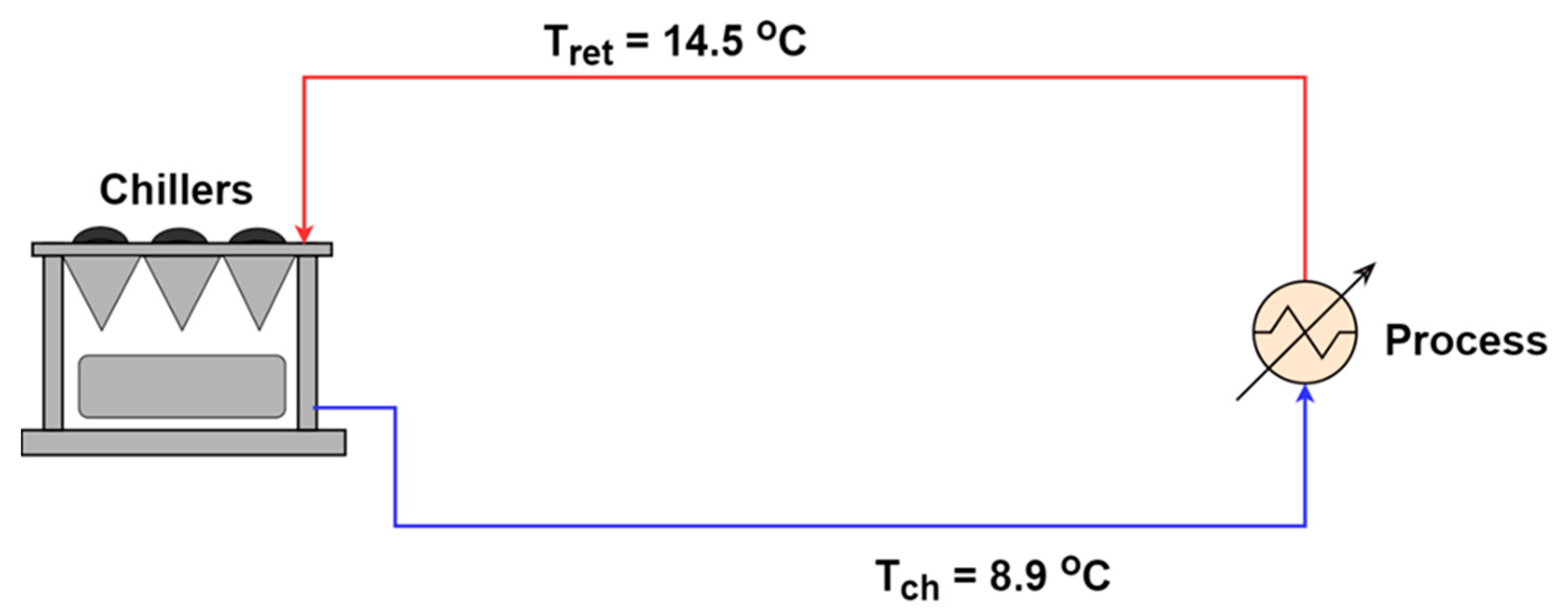
The facility uses air-cooled chillers to provide a continuous cooling load to the manufacturing process every day. The chillers provide chilled water at a temperature of 8.9 °C and a flowrate of 37.4 kg/s. The temperature difference across the chillers is ∆T = 5.6 °C and the return water temperature is 14.5 °C. This study compares three different scenarios for the process scheme with two of them having TES employed.

In the first scenario, “Baseline process”, the chillers provide the required cooling load (kWth) to the process. It is assumed that the process cooling load is constant and the chillers directly match the cooling load by varying their VFDs throughout the day as shown in Figure 1.

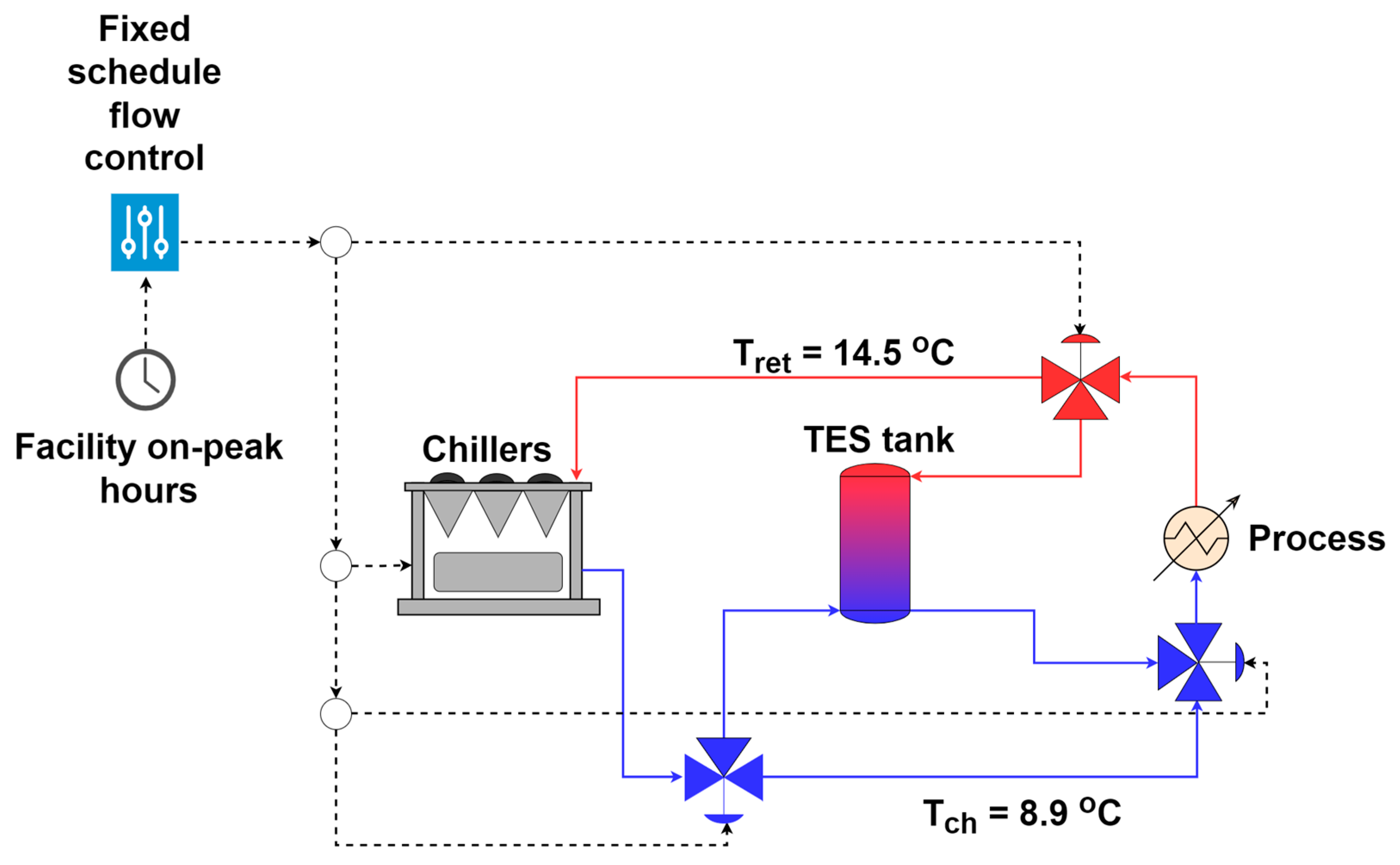
The second scenario, “Fixed schedule discharge”, utilizes TES to provide the cooling load (kWth) during on-peak hours. During off-peak hours, the chillers charge the tank and provide the required cooling to the process in which the chillers are using more electric load (kWe) to do both.

The fixed schedule of discharging and charging varies based on the electric rate schedule of the facility, which is set by the electric utility provider (as described in Section 2.3). Different rate schedules determine when facilities undergo schedules for on-peak and off-peak hours. For the facility studied in this paper, their rate schedule has on-peak hours occurring for seven hours divided into two different periods (from 6 a.m. to 9 a.m. and from 6 p.m. to 10 p.m.) during the months from October to May referred to as the winter schedule. During the months from June to September, the on-peak hours occur as seven continuous hours from 3 p.m. to 10 p.m. and this schedule is referred to as the summer schedule. During the winter schedule, the tank can serve the cooling load (kWth) to the process during the two different on-peak hour periods. During the summer schedule, the tank provides 60% of the required cooling load (kWth) to the process and the rest is provided by the chillers. The “Fixed schedule discharge” scenario has a logic controller as shown in Figure 2 that changes its action according to the fixed schedule discussed above. The controller charges the tank during off-peak hours in which the chillers use around double the usual electric load (kWe) to charge the tank and provide the cooling load (kWth) to the process.

The controller discharges the tank and turns off the chillers during on-peak hours of the winter schedule and relies solely on the tank to provide the cooling load (kWth) to the process. During the summer schedule, the controller ramps down the chillers to provide 40% of the cooling load (kWth) and the rest is supplied by the tank to meet the required cooling load of the process.

If the tank is fully charged, the controller will operate the process under the baseline process scenario during off-peak hours.

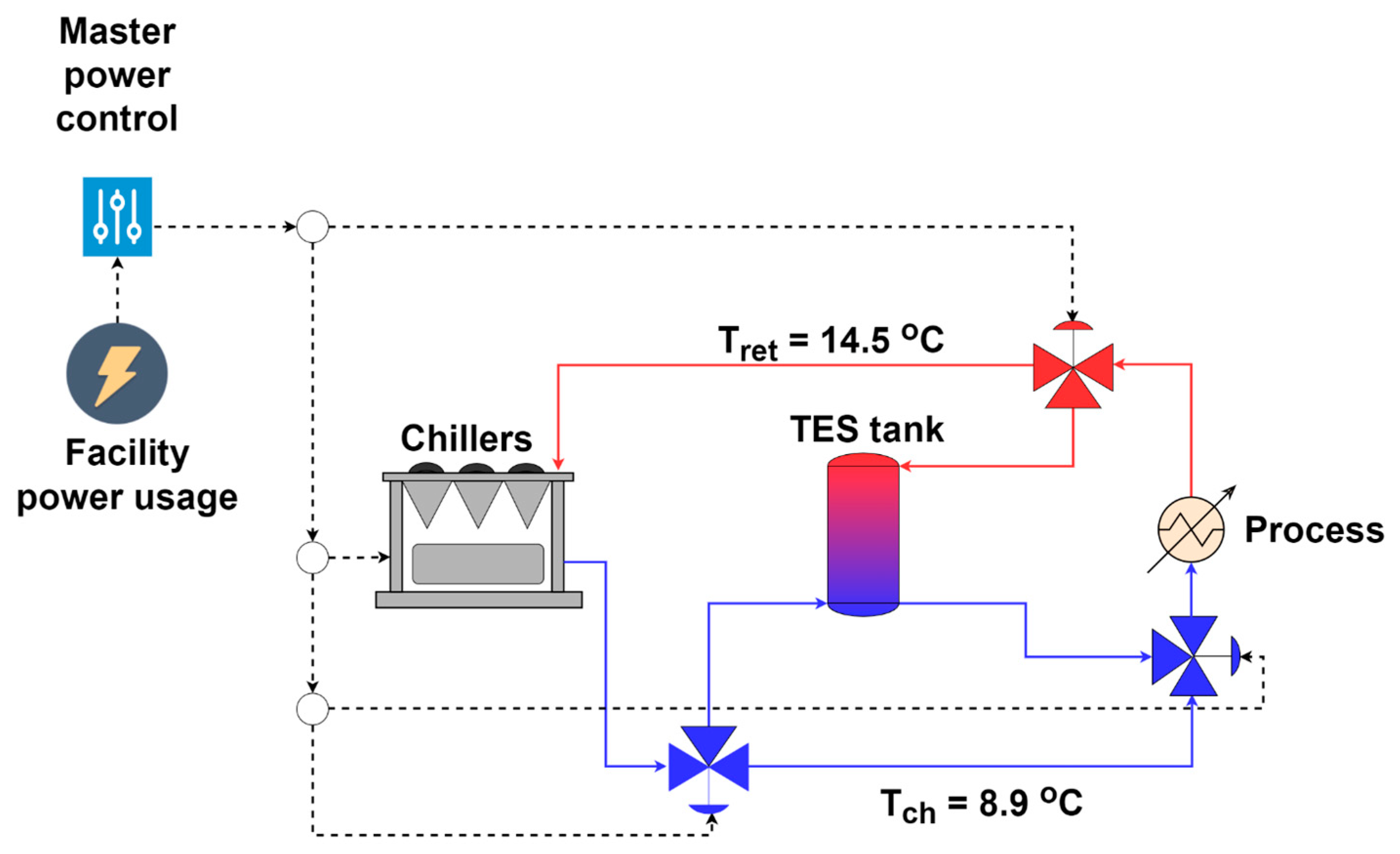
“Smart discharging” employs a smart controller as shown in Figure 3 to manipulate the VFDs of the chillers based on the facility’s real-time demand and the setpoint given to the controller, allowing for flexible charging and discharging of the tank. The control actions in this scenario differ from the “Fixed schedule discharge” scenario. The charging and discharging rates are not constant and can be adjusted based on the current power usage of the facility and the deviation from the setpoint.

Charging of the tank occurs when the facility’s power consumption is less than the setpoint of the controller; in this case, the chillers are using more load to charge the tank and provide the required cooling load (kWth) to the process. The electric load (kWe) used to charge the tank is equal to the difference between the setpoint and the transmitter reading.

Discharging of the tank occurs when the facility’s power consumption is higher than the setpoint and the difference between them is high enough that the controller will turn off the chillers and utilize the tank to provide the required cooling load (kWth) to the process.

Smart discharging occurs when the difference between the transmitter reading and the setpoint is not high enough. To meet the setpoint, the controller will ramp down the chiller load and discharge the tank with the difference between the transmitter reading and the setpoint to provide the required cooling load (kWth) to the process using both the chillers and the tank.

If the facility power consumption is equal to the setpoint or the tank is fully charged, the smart controller will employ the baseline process scenario.

The setpoints are chosen based on the historical data provided by the facility, with each month having its setpoint. The setpoint is chosen so that it avoids the over-discharge of the tank and, in this case, the chillers will use more electric load (kWe) to charge the tank, which will increase the facility’s power usage, or the process will be forced to follow the baseline scheme because the tank cannot provide the required cooling load (kWth). In the instance of choosing a high setpoint, this will lead to losing some potential savings from using the tank to achieve demand charge savings.

2.2. TES Tank Modeling

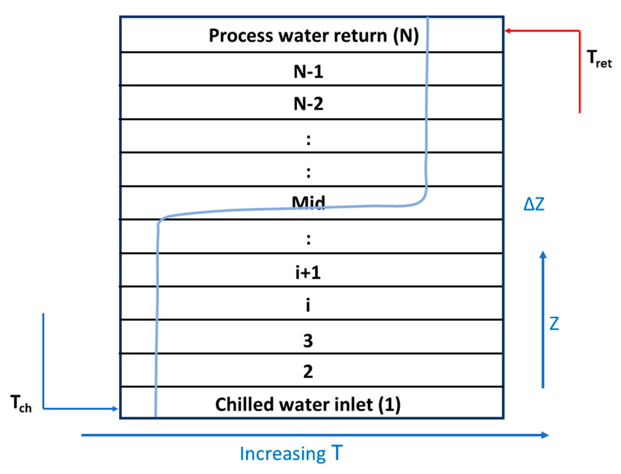
TES tank modeling has been studied by various researchers and different modeling approaches have been proposed using a varying number of nodes [33,34,35,36]. The accuracy of temperature profiles and the issue of numerical diffusion are greatly influenced by the number of nodes used. An increase in the number of nodes reduces the numerical diffusion effect but also leads to longer simulation times [33,34]. To investigate the impact of numerical diffusion, researchers have employed various numbers of nodes and observed the effect on the temperature profiles. In our study, a one-dimensional model equation with 100 nodes is used in this study to simulate the temperature variations at each node of the TES tank and generate a temperature profile. Equation (1) is used to model the temperature of the tank at each node:

$${\mathsf{\rho }}_{\mathrm{i}}{\mathrm{C}}_{\mathrm{p}}\mathrm{A}∆\mathrm{z}\frac{\mathrm{d}{\mathrm{T}}_{\mathrm{i}}}{\mathrm{d}\mathrm{t}}=\mathrm{U}\mathrm{P}\left({\mathrm{T}}_{\mathrm{a}\mathrm{m}\mathrm{b}}-{\mathrm{T}}_{\mathrm{i}}\right)+\frac{\mathrm{k}\mathrm{A}}{∆\mathrm{z}}\left({\mathrm{T}}_{\mathrm{i}-1}-2{\mathrm{T}}_{\mathrm{i}}+{\mathrm{T}}_{\mathrm{i}+1}\right)+{\mathrm{ṁ}}_{\mathrm{c}\mathrm{h}}{\mathrm{C}}_{\mathrm{p}}\left({\mathrm{T}}_{\mathrm{i}-1}-{\mathrm{T}}_{\mathrm{i}}\right)+{\mathrm{ṁ}}_{\mathrm{d}\mathrm{s}\mathrm{c}\mathrm{h}}{\mathrm{C}}_{\mathrm{p}}\left({\mathrm{T}}_{\mathrm{i}+1}-{\mathrm{T}}_{\mathrm{i}}\right)$$

(1)

The energy rate of change for each node is represented by the term on the left hand side of the equation, which depends on several factors, including the density of water at node (i) denoted as ${\mathsf{\rho }}_{\mathrm{i}}$[37] in which the density varies with the temperature; the specific heat capacity of water denoted as C_p [37]; the incremental height ∆z, which is the height of each node calculated using the tank height Z and the number of nodes N, also plays a role in this term and is calculated in Appendix A. On the right-hand side of the equation, the first term represents the heat loss to the ambient air, where U is the overall heat transfer coefficient to the ambient air [19] and P is the perimeter of the node. The second term represents heat transfer by conduction, with k representing the thermal conductivity coefficient [37]. The last two terms represent the energy of charging and discharging the chilled water going to the process. These two energies are calculated based on upwind energy balance calculations. The (i − 1) node appears in the charging term because the flow is upward, so the upwind node here is (i − 1) with reference to (i), while (i + 1) is used for discharging because of the downward flow, so the upwind node is (i + 1) with reference to (i). Equations (2) and (3) calculate the temperatures at the bottom and top nodes, respectively, which are the boundaries of the tank. The coefficient $\frac{4}{3}$ arises from the assumption that the wall temperature is equal to the water temperature, with the wall being located at a distance of $\frac{∆\mathrm{z}}{2}$, leading to the usage of the mentioned coefficient [34].

$${\mathsf{\rho }}_1{\mathrm{C}}_{\mathrm{p}}\mathrm{A}∆\mathrm{z}\frac{\mathrm{d}{\mathrm{T}}_1}{\mathrm{d}\mathrm{t}}={\mathrm{U}}_1\mathrm{P}\left({\mathrm{T}}_{\mathrm{a}\mathrm{m}\mathrm{b}}-{\mathrm{T}}_1\right)+\frac{4}{3}\frac{\mathrm{k}\mathrm{A}}{∆\mathrm{z}}\left({\mathrm{T}}_2-{\mathrm{T}}_1\right)+{\mathrm{ṁ}}_{\mathrm{c}\mathrm{h}}{\mathrm{C}}_{\mathrm{p}}\left({\mathrm{T}}_{\mathrm{c}\mathrm{h}}-{\mathrm{T}}_1\right)+{\mathbf{ṁ}}_{\mathrm{d}\mathrm{s}\mathrm{c}\mathrm{h}}{\mathrm{C}}_{\mathrm{p}}\left({\mathrm{T}}_2-{\mathrm{T}}_1\right)$$

(2)

$${\mathsf{\rho }}_{\mathrm{N}}{\mathrm{C}}_{\mathrm{p}}\mathrm{A}∆\mathrm{z}\frac{\mathrm{d}{\mathrm{T}}_1}{\mathrm{d}\mathrm{t}}={\mathrm{U}}_{\mathrm{N}}\mathrm{P}\left({\mathrm{T}}_{\mathrm{a}\mathrm{m}\mathrm{b}}-{\mathrm{T}}_{\mathrm{N}}\right)+\frac{4}{3}\frac{\mathrm{k}\mathrm{A}}{∆\mathrm{z}}\left({\mathrm{T}}_{\mathrm{N}}-{\mathrm{T}}_{\mathrm{N}-1}\right)+{\mathrm{ṁ}}_{\mathrm{c}\mathrm{h}}{\mathrm{C}}_{\mathrm{p}}\left({\mathrm{T}}_{\mathrm{N}-1}-{\mathrm{T}}_{\mathrm{N}}\right)+{\mathbf{ṁ}}_{\mathrm{d}\mathrm{s}\mathrm{c}\mathrm{h}}{\mathrm{C}}_{\mathrm{p}}\left({\mathrm{T}}_{\mathrm{r}\mathrm{e}\mathrm{t}}-{\mathrm{T}}_{\mathrm{N}}\right)$$

(3)

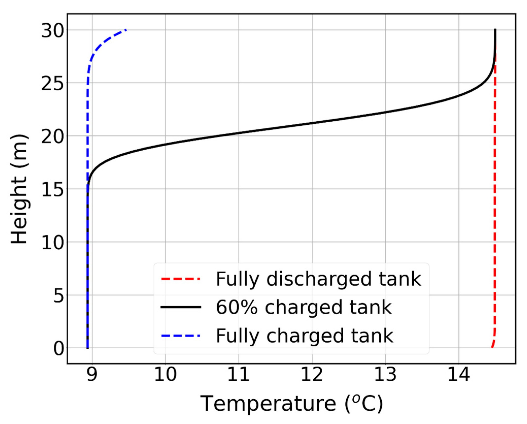
The parameters used in the three equations are listed in Appendix A. The tank model uses N = 100 nodes in which the numerical diffusion does not have a significant impact and, at the same time, the simulation time is about 15 min. For further clarifications and comparisons of results obtained by varying node numbers, refer to previous studies [33,34]. A graphical representation of the tank temperature profile as a function of height is shown in Figure 4 and Figure 5.

The charging temperature of the tank is 8.9 °C while the return temperature from the process to the tank is 14.5 °C. The tank is designed to meet the process cooling requirements for a duration of 4 h, which are the on-peak hours (Section 2.3). As a result, it has a height of 21.5 m and a diameter of 5.7 m. The height and diameter are determined using the typical industrial aspect ratio AR = 3.8, which is the ratio between the height and the diameter [38].

2.3. Facility Data

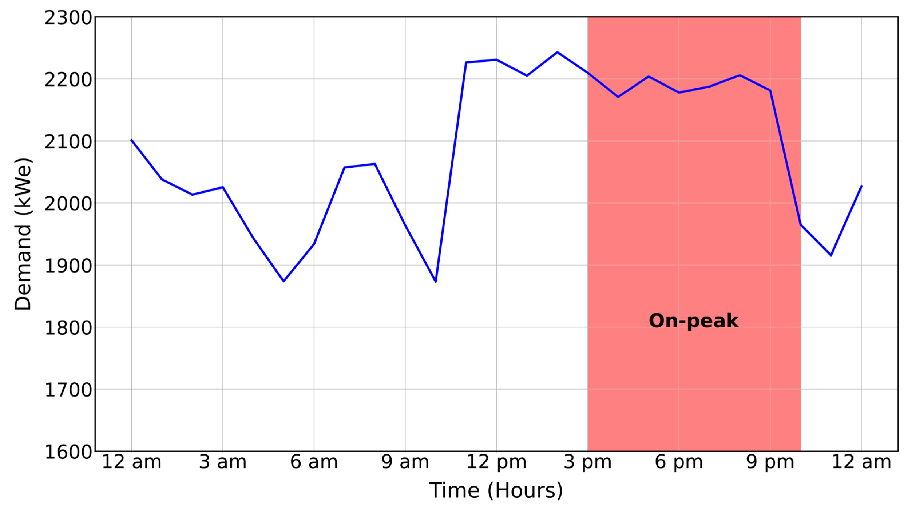
This study utilizes utility data obtained from the facility for 2022 year total energy usage. The data provided by the facility include the electricity usage in kilowatt-hours (kWh) totaled every 15 min. The specific charges for each category according to the facility’s rate schedule are presented in

Table 2. Facility’s charges’ description with the on-peak and off-peak schedule according to the utility provider, which is Rocky Mountain Power.

Charges Category	Cost (USD)
On-peak demand	USD 14.96 per kW from October to May
	On-peak hours from 6 am to 9 a.m. and from 6 p.m. to 10 p.m. except on weekends
	USD 16.61 per kW from June to September
	On-peak hours from 3 p.m. to 10 p.m. except on weekends
kWh off-peak	USD 0.02316 per kWh from October to May
	USD 0.0262 per kWh from June to September
kWh on-peak	USD 0.04556 per kWh from October to May
	USD 0.0515 per kWh from June to September

. The cooling load (kWth) required for the facility’s process is estimated to be 873 kW, based on on-site data collection. Figure 6 provides an example of a facility demand profile on a representative day in the summer schedule, with the shaded area representing the kW values for on-peak hours, and the area under the curve here would be kWh usage during on-peak hours. Using the same means, off-peak kWh usage can be calculated. On-peak demand charges are calculated using the peak kW usage during on-peak hours multiplied by the charges of the facility, which are listed in Table 2.

2.4. Chiller Model

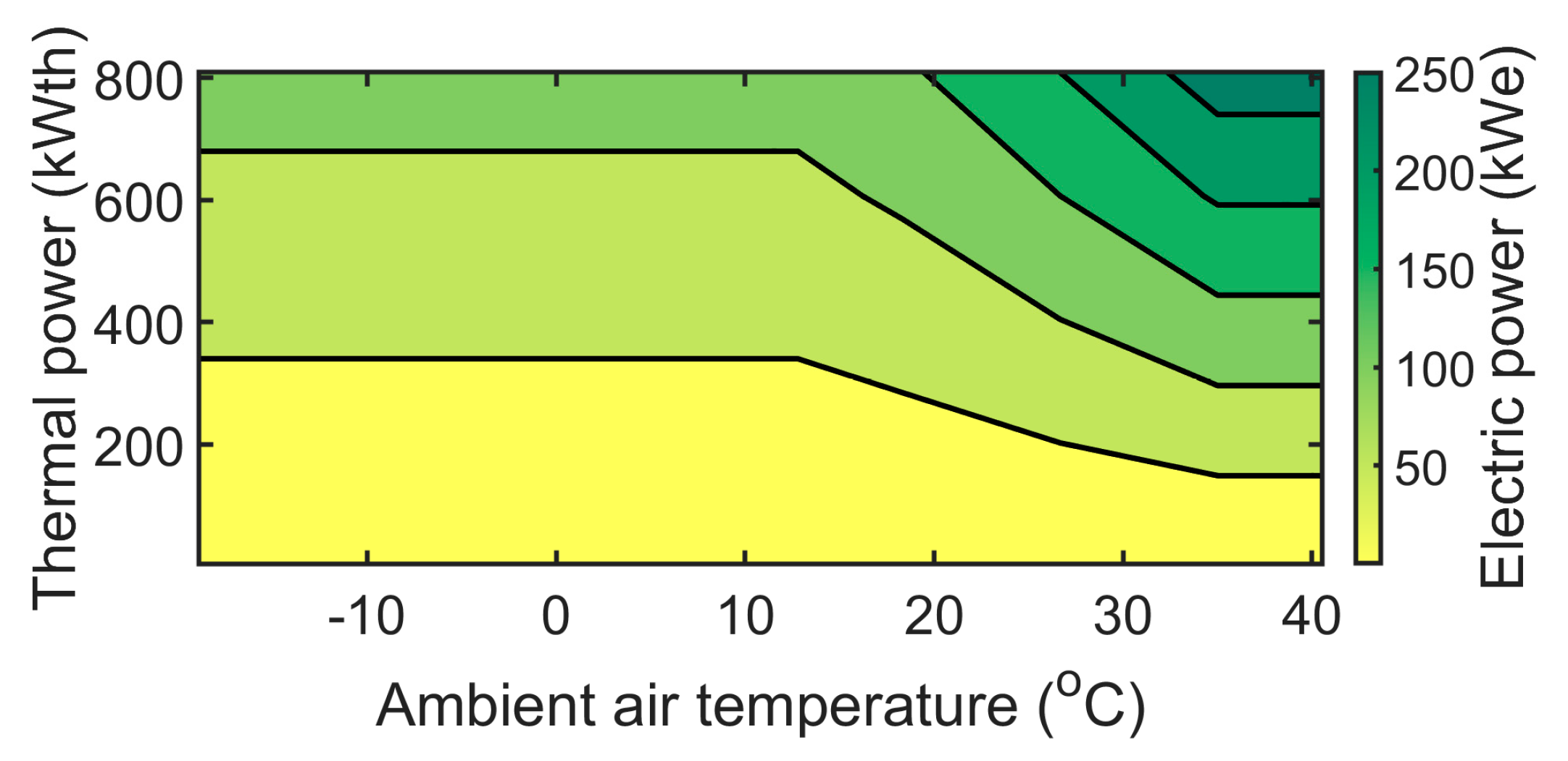
The chillers in this facility are air-cooled chillers with VFDs on their compressors. In this study, the chiller model is created based on the chiller datasheet provided by the facility (

Table 3. The datasheet of the chiller provided by the facility.

Ambient Air Temperature (°C)	Thermal Power (kWth)	Electrical Power (kWe)
35	809	274
27	607	149.5
18	404	71
13	202	29.8

). The model utilizes ambient air temperature as an independent variable to calculate the electric load in (kWe) required by the chiller based on the cooling needs (kWth) of the facility. The chiller’s electric load (kWe) and thermal load (kWth) are directly proportional to ambient air temperature, with higher temperatures requiring more electric power (kWe) from the chiller to meet the cooling load (kWth).

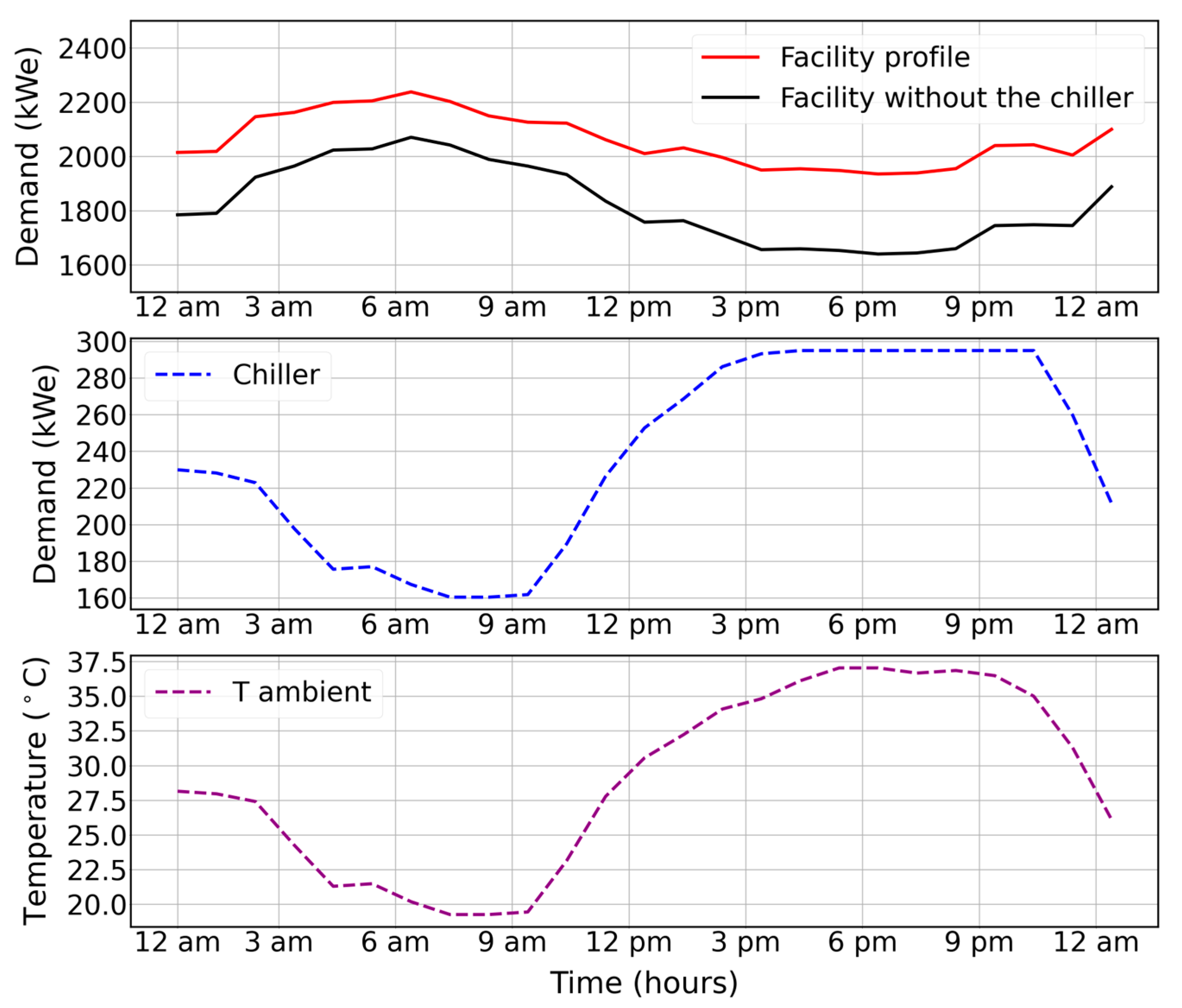
The chiller model is created using a 2D interpolation function to generate a load profile for the chiller based on the ambient air temperature and the required cooling load for the process, as shown in Figure 7. The model provides upper and lower limits for kWe usage, regardless of variations in ambient air temperature. This model is a critical parameter in achieving results and savings for the case study, as the chillers use more kWe during off-peak hours to charge the tank and less power during on-peak hours when the tank provides the necessary cooling load (kWth) to the process. The chiller model plays a crucial role in both the “Fixed schedule discharge” and “Smart discharging” process schemes discussed in Section 2.1. After creating the chiller model and generating a load profile for the entire study period, a baseline is established by subtracting the chiller load profile from the facility profile data to be used in the two proposed scenarios calculations, as demonstrated in Figure 8. The three process scenarios along with the TES tank are simulated using Simulink in MATLAB with solver ode23s.

3. Results

3.1. “Fixed Schedule Discharge” vs. “Baseline Process”

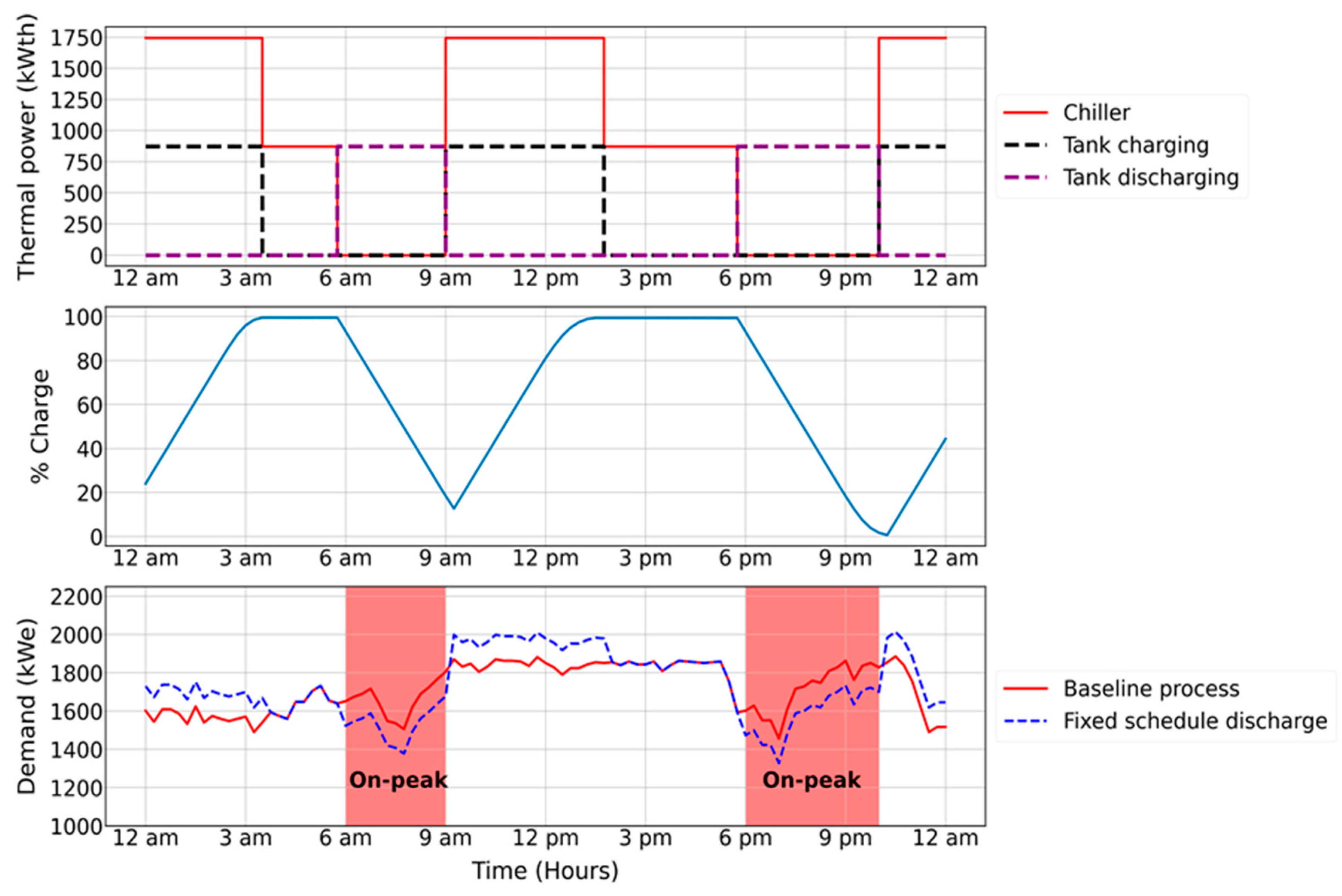
The simulation of the “Fixed schedule discharge” scheme results in demand charge savings during on-peak hours, as shown in Figure 9. These savings are reflected in the total charges for the facility, as shown in

Table 4. Fixed schedule discharge vs. baseline process charges in January.

Category\Scenario	Baseline Process	Fixed Schedule Discharge	Percent Saved
On-peak demand charges	USD 31,722	USD 29,801	6%
Energy charge kWh off-peak	USD 24,671	USD 25,537	−3.5%
Energy charge kWh on-peak	USD 14,062	USD 12,949	8%
Total charges	USD 70,455	USD 68,288	3%

. Figure 9 displays the results of a one-day simulation in January of the facility profile using both the “Baseline process” and “Fixed schedule discharge” schemes. The plot illustrates that the “Fixed schedule discharge” scheme consumes more electric power during off-peak hours when the chillers are charging the tank and providing the cooling load (kWth) to the process. However, during on-peak hours, the facility uses significantly less electric power because the chillers are turned off, and the tank provides the cooling load to the process. The shaded area represents the on-peak hours. Figure 9 shows how the percent charge of the tank aligns with the flowrates of the chillers and the process. As discussed in Section 2.1, if the tank is charging, the chillers provide the cooling load to the process and charge the tank.

If the tank is full, the chillers provide the cooling load to the process only. If the tank is discharging, the chillers are turned off, and the tank provides the cooling load. The chillers provide double the cooling load required during charging to charge the tank and provide the required cooling load to the process. The facility profile also aligns with the TES percent charge plot, in which if the tank is charging, the “Fixed schedule discharge” profile is higher and vice versa during discharging. Table 4 shows the distribution of the three categories included in the calculation of the total monthly facility charges. It demonstrates the savings provided by implementing the “Fixed schedule discharge” scheme in January.

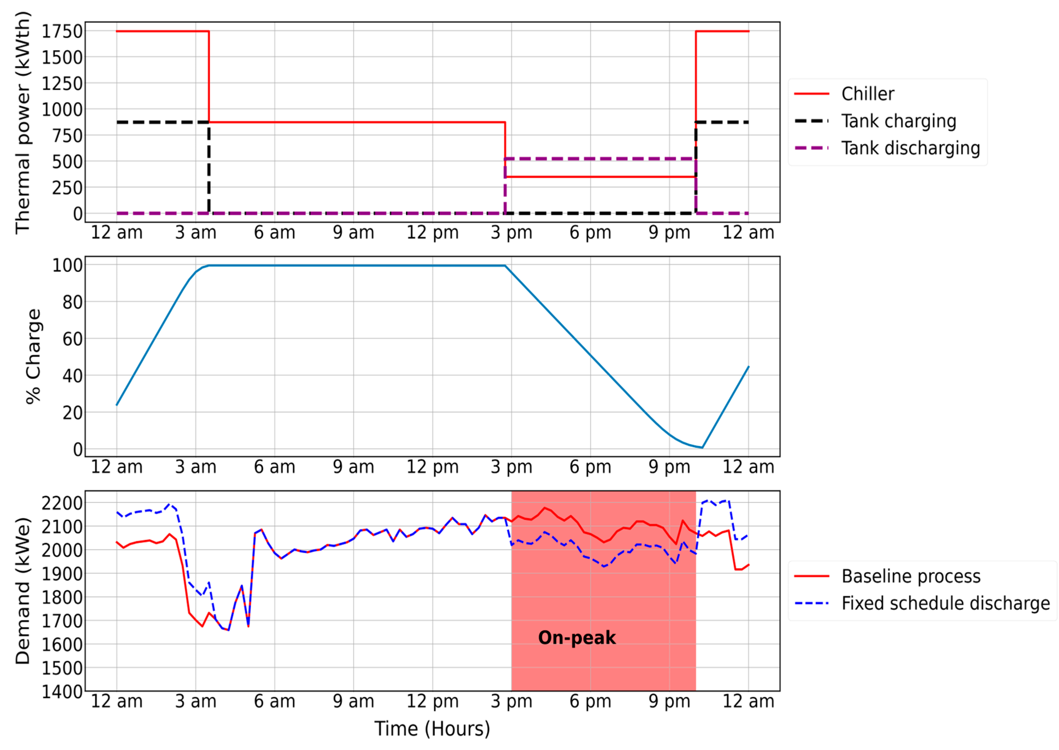
Figure 10 and

Table 5. Fixed schedule discharge vs. baseline process charges in June.

Category\Scenario	Baseline Process	Fixed Schedule Discharge	Percent Saved
On-peak demand charges	USD 37,575	USD 35,357	6%
Energy charge kWh off-peak	USD 27,353	USD 28,442	−4%
Energy charge kWh on-peak	USD 18,807	USD 17,085	9%
Total charges	USD 83,734	USD 80,885	3.5%

show the results of simulating the same scenario for one day in June and the monthly charges of the facility. The on-peak hours in June follow the summer schedule, which affects the electric power usage of the chillers and the demand profile of the facility because the chillers are not turned off in the summer schedule. It is evident from Table 4 and Table 5, and Figure 9 and Figure 10 that the savings result from shifting the load from on-peak to off-peak hours. The “Fixed schedule discharge” scheme has lower kW and kWh on-peak charges, but higher kW and kWh off-peak charges. The primary parameter here is that the demand charges for kW during on-peak hours are more expensive than those for the off-peak kWh, and there are no charges for off-peak kW demand. This is how the savings arise from implementing this scenario.

3.2. “Smart Discharging” vs. “Baseline Process”

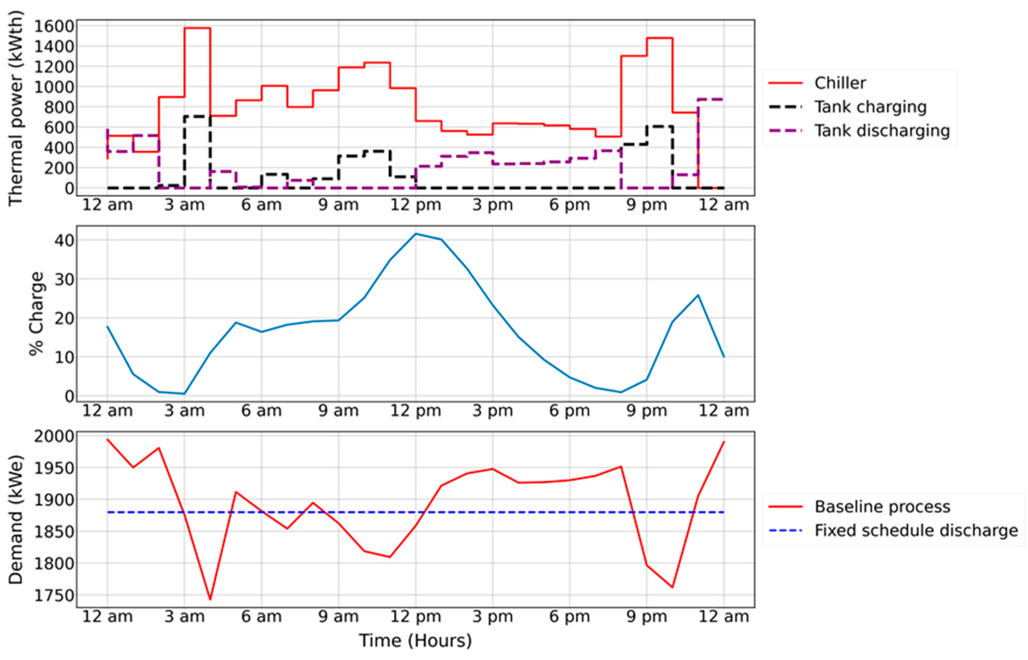
The “Smart discharging” scenario utilizes a dynamic and flexible smart controller that reacts based on the real-time facility demand and the setpoint given. Unlike the “Fixed schedule discharge” scheme, this scenario does not have a fixed schedule for charging and discharging. Figure 11 shows the facility profile for one day in January with the percent charge and thermal power (kWth).

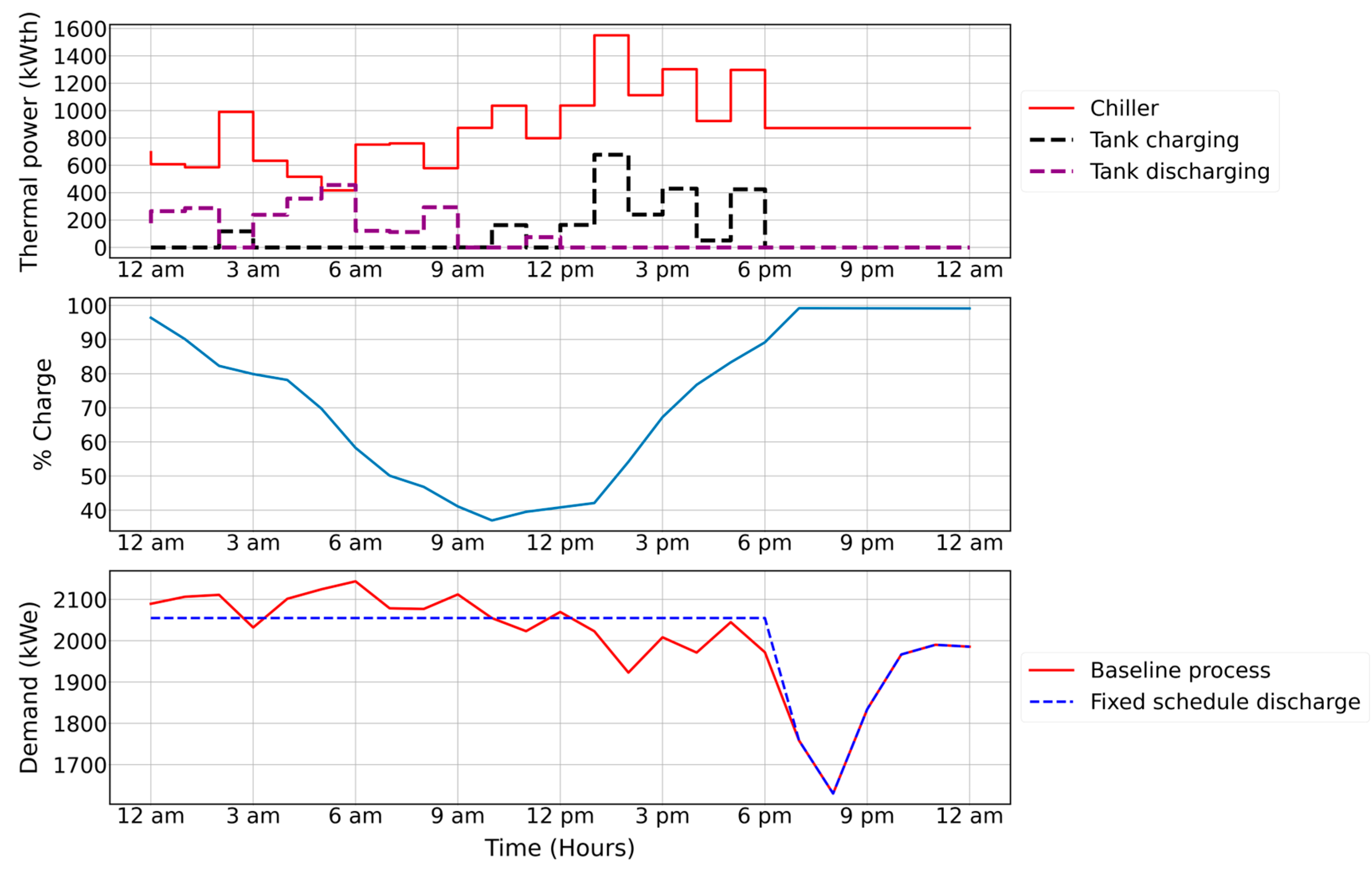
Figure 12 shows the results for the same scenario in June. The same figure shows some instances when the new facility profile drops to the baseline demand profile. This occurs if the tank is fully charged, so the controller utilizes the baseline process scenario. Looking at the monthly facility charges and the savings provided by “Smart discharging”,

Table 6. Smart discharging vs. baseline process charges in January.

Category\Scenario	Baseline Process	Smart Discharging	Percent Saved
On-peak demand charges	USD 31,722	USD 29,801	6%
Energy charge kWh off-peak	USD 24,671	USD 24,284	1.5%
Energy charge kWh on-peak	USD 14,062	USD 14,040	0.2%
Total charges	USD 70,455	USD 68,124	3.5%

and

Table 7. Smart discharging vs. baseline process charges in June.

Category\Scenario	Baseline Process	Smart Discharging	Percent Saved
On-peak demand charges	USD 37,575	USD 34,474	8%
Energy charge kWh off-peak	USD 27,353	USD 27,293	0.2%
Energy charge kWh on-peak	USD 18,807	USD 18,126	3.5%
Total charges	USD 83,734	USD 79,892	4.5%

present the distribution of charges for the months of January and June, respectively, showing the savings provided by implementing this scheme. The setpoints chosen for each month are listed in

Table 8. The setpoints for each month for Smart discharging scenario.

Month	Setpoint kW
January	1880
February	1920
March	1900
April	1970
May	1970
June	2055
July	2240
August	2280
September	2270
October	2000
November	1970
December	1880

. These setpoints are estimated using historical data provided by the facility to optimize savings and maintain the tank storage of chilled water to sustain production throughout the month. For instance, if the operator selects a low setpoint, the tank will be over-discharged before the end of the month. Conversely, if a high setpoint is chosen, the facility will incur additional charges as it will not receive the optimum savings from using the tank.

4. Discussion

4.1. Comparison between the Three Different Scenarios

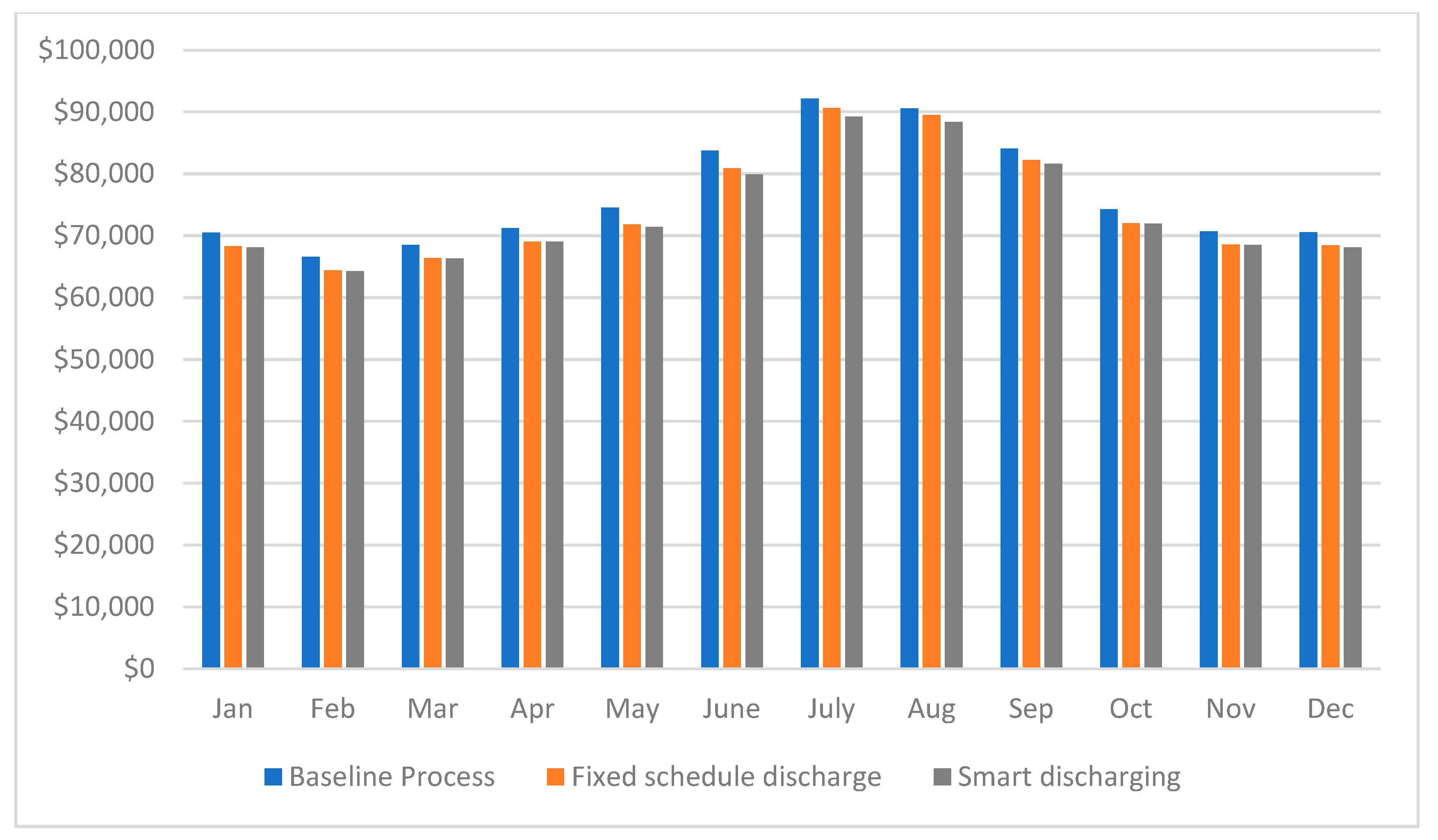
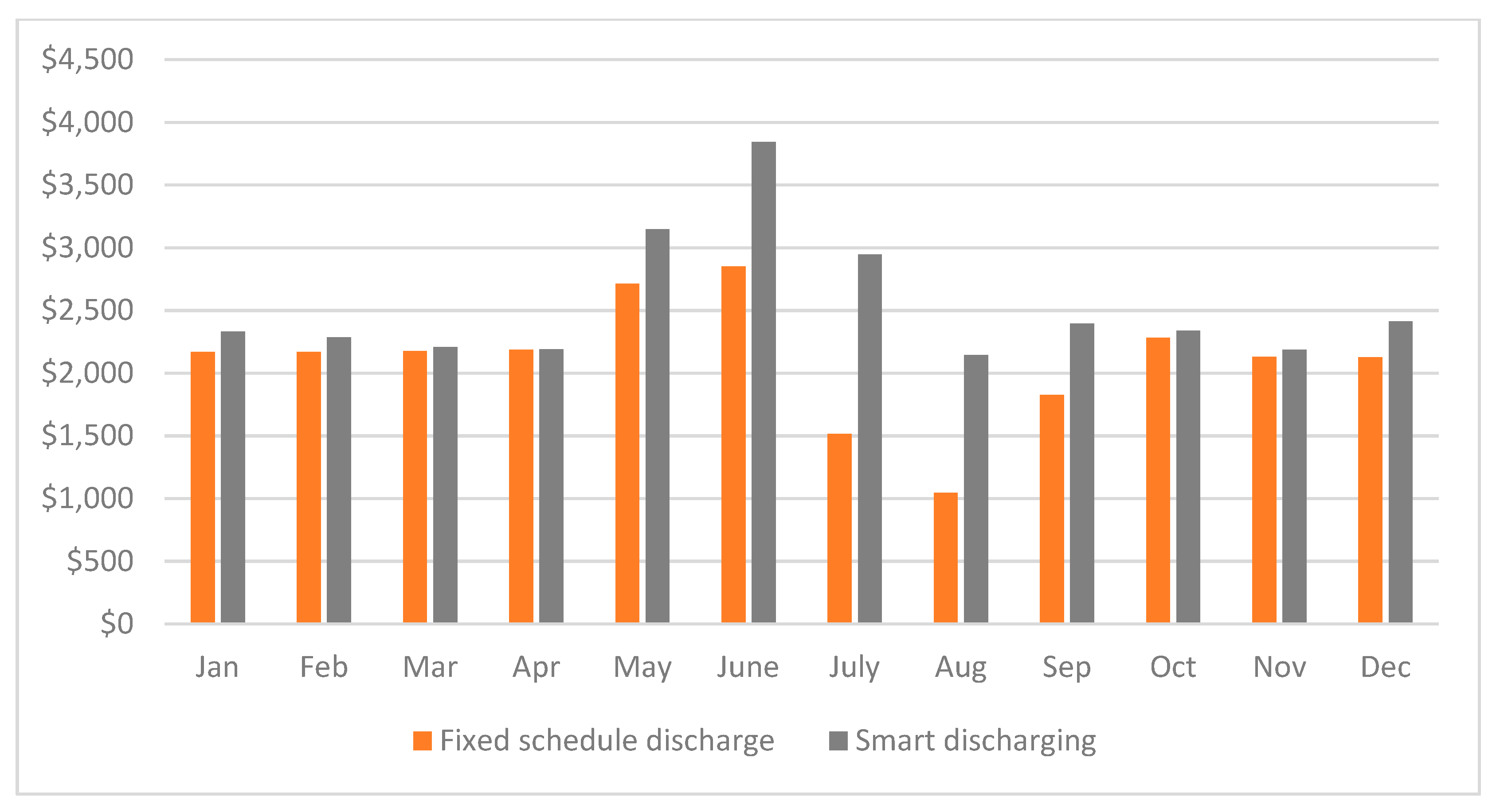
This section presents a comprehensive comparison of the results obtained from the three different scenarios with respect to their total charges, highlighting the superior cost-effectiveness of the “Smart discharging” scheme. The monthly total charges of the facility for the simulation period of 2022 year are presented in Figure 13, which indicates that the “Smart discharging” scheme incurred the lowest charges throughout the period. Figure 14 and

Table 9. Comparative analysis for the two proposed scenarios for each month.

Savings\Scenarios	Fixed Schedule Discharge	Smart Discharging
January	USD 2167	USD 2331
February	USD 2167	USD 2284
March	USD 2176	USD 2209
April	USD 2185	USD 2189
May	USD 2711	USD 3146
June	USD 2849	USD 3842
July	USD 1515	USD 2947
August	USD 1045	USD 2142
September	USD 1826	USD 2395
October	USD 2280	USD 2339
November	USD 2131	USD 2186
December	USD 2125	USD 2413

show a comparison between the savings achieved by implementing the “Smart discharging” scheme and “Fixed schedule discharge” scheme. The savings provided by “Smart discharging” were found to be higher due to the flexibility of the “Smart discharging” scheme in charging and discharging, which played a significant role in achieving these savings compared to the constant charging and discharging scheduling of the “Fixed schedule discharge” scheme. Furthermore,

Table 10. Total charges for each scenario.

Scenarios	Baseline Process	Fixed Schedule Discharge	Smart Discharging
Total charges	USD 917,255	USD 892,078	USD 886,832

provides an overview of the total charges of the facility for each scenario.

4.2. Payback Period for Using the Two Proposed Process Schemes

The tank volume was determined based on the facility data and the winter schedule’s on-peak hours, as discussed in Section 2.3. The tank was sized to provide cooling to the process during the four on-peak hours when the chillers are turned off. The cost of designing the tank can be estimated based on the cooling load in ton-hour units, which can be calculated by multiplying the kWth cooling provided by the tank by the number of hours, which is four in this case. The estimated cooling load in ton-hours for the tank is 992 ton-hours. The tank would cost around USD 200,000, which is calculated as USD 200 per ton-hour multiplied by 992 ton-hours [39]. Incentives are available for TES applications provided by different utility providers to encourage facilities to implement these applications and facilitate the process of grid production.

Table 11. Payback period for using smart discharging and fixed schedule discharge.

Scenario	Cost (USD)	Savings (USD)	Payback Years
Fixed schedule discharge	USD 200,000	USD 25,100	8
Smart discharging	USD 200,000	USD 30,400	6.5

shows the calculated payback period for the two proposed scenarios without incentives.

4.3. Sensitivity Analysis

4.3.1. Setpoint vs. Cost Savings

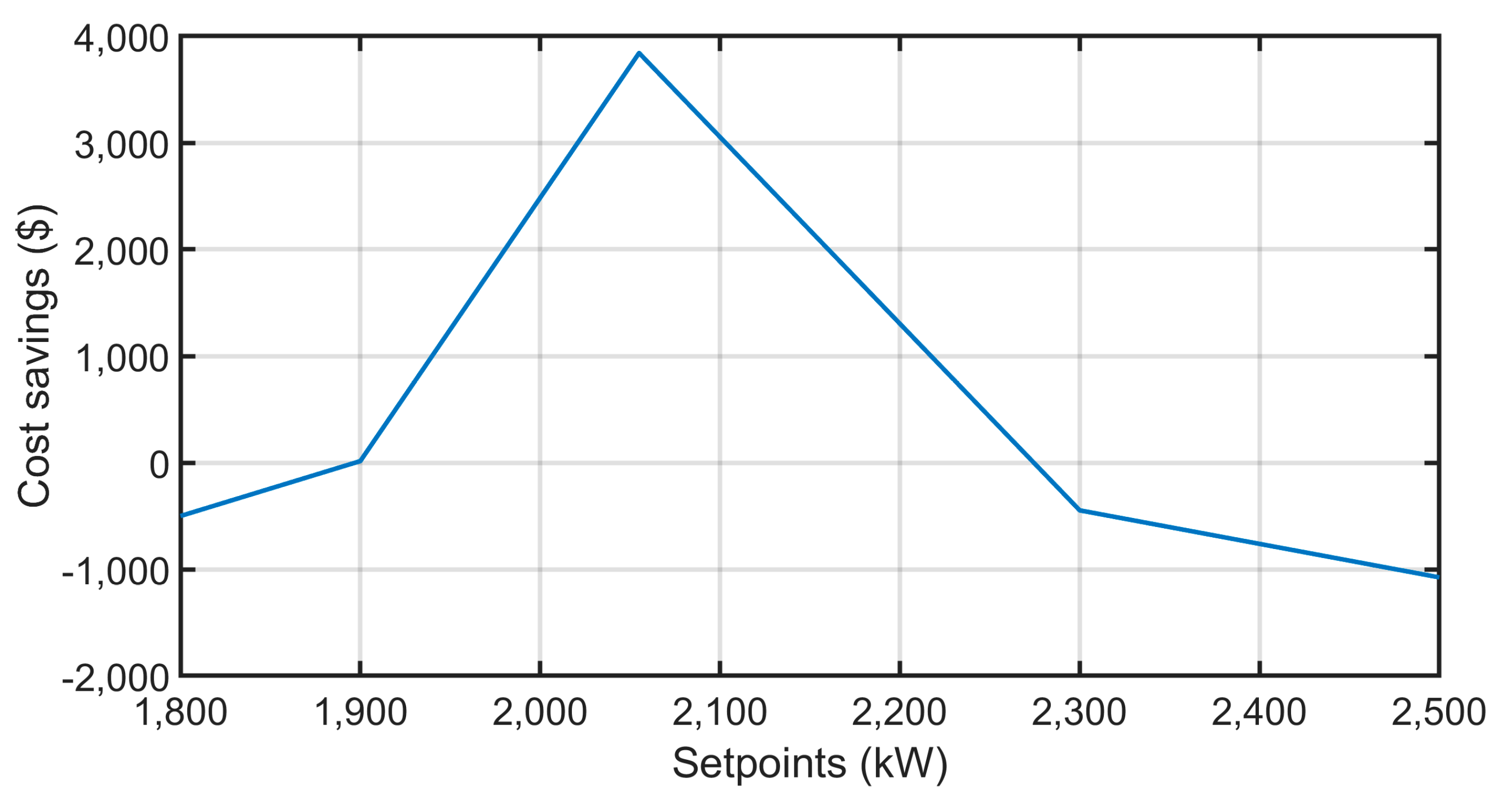
The process of estimating the setpoint for each month is very critical to achieve optimum savings. As shown in Figure 15, the change in the controller setpoint will deeply affect the cost savings each month, in which having a higher setpoint will lead to more charges because the facility will not be benefiting most from using the tank. On the other hand, choosing a lower setpoint will lead to over-discharge of the tank and the facility may have zero savings and even pay more because the chillers will charge the tank during times when they are not supposed to.

4.3.2. Size of the Tank vs. Cost Savings

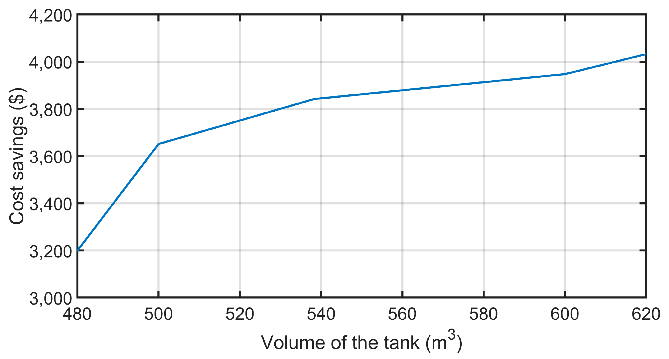
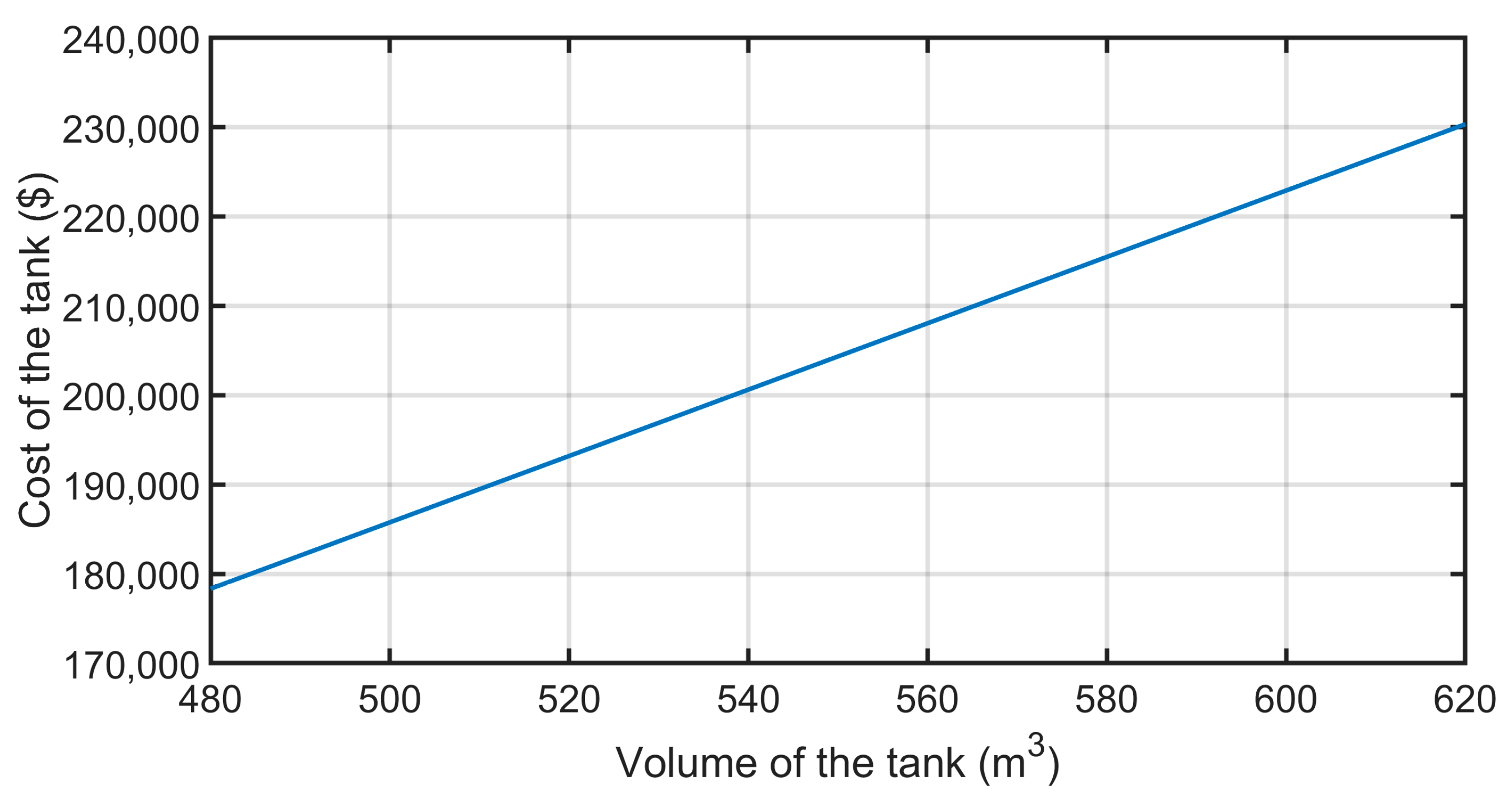
Changing the size of the tank will not have a remarkable impact on cost savings. Having a larger tank will provide a larger capacity for storage, which will reduce the setpoint a little bit. Then, this will lead to more savings, but the additional savings are not significant. One important side to consider is that the size of the tank was estimated to supply the cooling load during the on-peak hours of the facility during the winter schedule. In this case, having a larger tank would not add anything for the “Fixed schedule discharge” scenario as the estimated size is already doing a good job. As shown in Figure 16, increasing the volume of the tank after a certain point would not be effective to increase the cost savings. Additionally, increasing the volume of the tank would lead to higher installation costs [39]. Figure 17 shows that the cost of installing a larger tank is very expensive compared to the additional savings achieved by it.

4.3.3. Utility Rates vs. Cost Savings

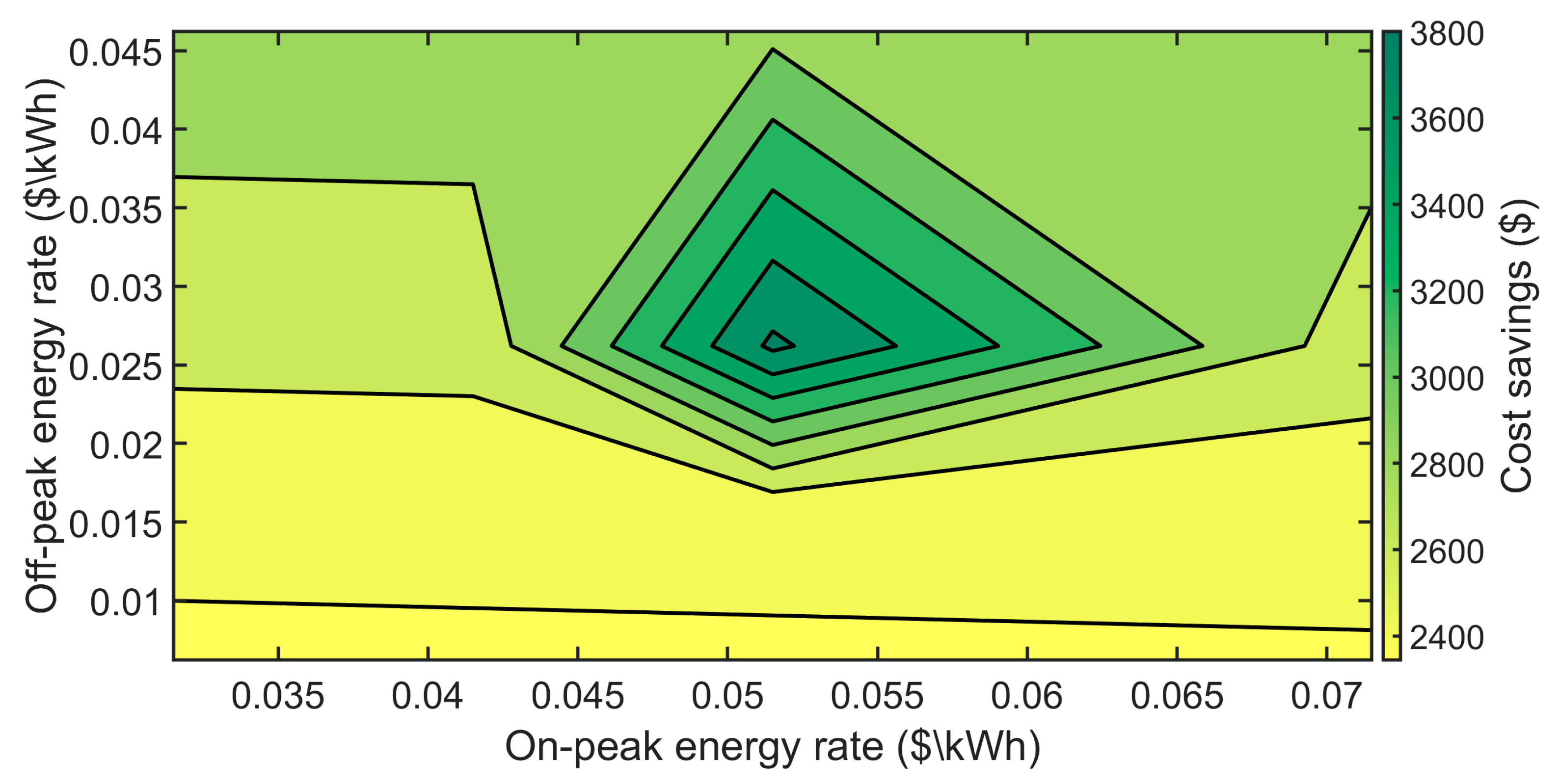
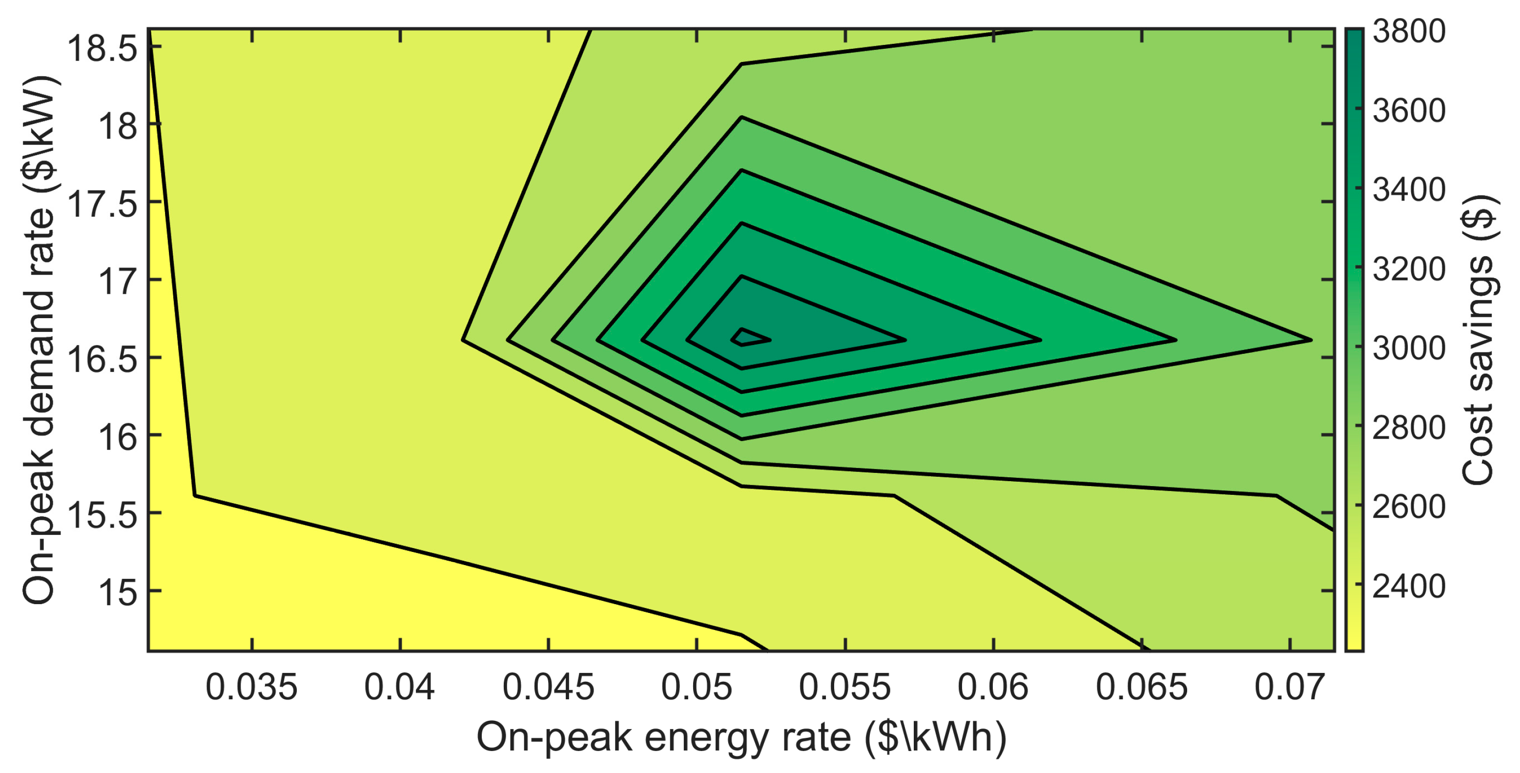
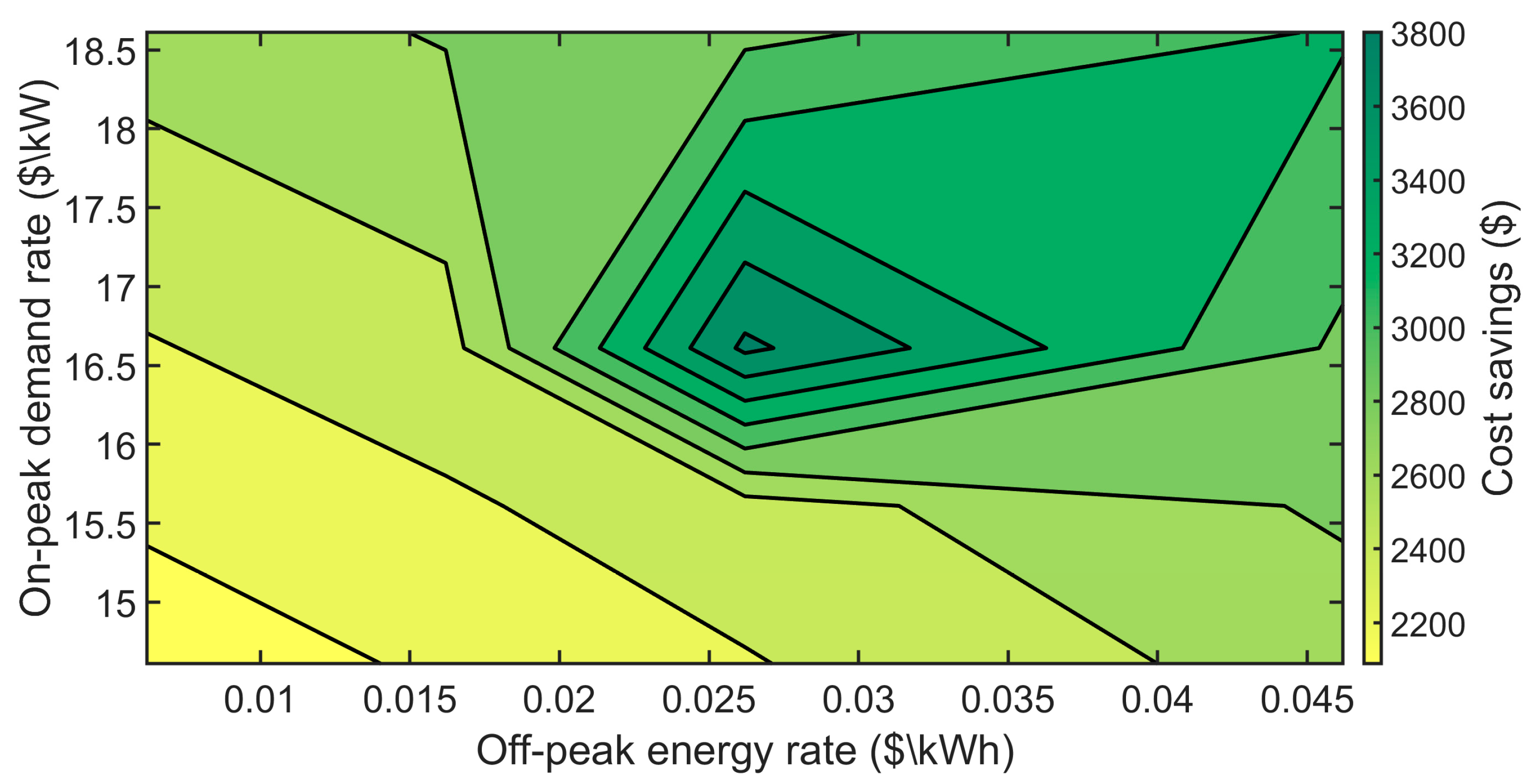
The results shown in the paper are based on the assumption of having a flat rate of utilities (Section 4.4). This section provides a sensitivity analysis to study the effect of changing the utility rates on the savings achieved by implementing the “Smart discharging” scenario during the summer schedule, specifically in June. Figure 18 shows the variation in the energy rates for on-peak USD/kWh and off-peak USD/kWh while fixing the demand charges at USD 16.61/kW (Section 2.3). Figure 19 depicts the same analysis but for the variation in the demand rates USD/kW and on-peak charges while fixing the off-peak charges at USD 0.0262/kWh. Figure 20 shows the variation in the demand rates USD/kW and off-peak charges while fixing the on-peak charges at USD 0.0515/kWh.

As shown in the three plots, it was expected that the variation in the demand rates USD/kW and on-peak charges USD/kWh (Figure 19) would have the highest impact among them. Because the demand rate was expensive, any change in the rate would have a significant impact on the savings. Regarding the energy rates, on-peak energy rates were more expensive than off-peak energy rates, which is why their impact was higher than the off-peak, but this does not mean that off-peak energy savings do not play an important role in the case of the “Smart discharging” scenario (Results, Section 3.2).

4.4. Limitations, Assumptions, and Challenges

The assumptions used here are as follows:

• Having a flat utility rate for energy and demand charges;
• The process cooling demand is not changing in terms of (kWth).

These assumptions can affect the impact of the TES, in which the demand charges would have an impact on the chosen setpoint and the rates of charging and discharging. Changing the process cooling demand will also have an impact on the charging and discharging of the tank and will thus change the optimum setpoint.

The limitations in this study are related to the storage tank—the space available to install the tank and the cost of installation of the tank. Having a larger tank will lead to more savings achieved for the “Smart discharging” scenario. Additionally, having a larger tank will require more installation costs, which is more significant than the savings achieved by installing a larger tank (Section 4.3.2). Moreover, installing a larger tank for “Fixed schedule discharge” will not affect the savings during the winter schedule, because the chillers are turned off and the tank solely provides the cooling load to the process. So, having a larger tank will not make any difference in this case. On the other hand, it could achieve more savings during the summer schedule, because the tank would have a larger capacity, which would help in reducing the electric load of the chillers. The volume of the tank was sized to meet the process cooling needs for the on-peak hours during the winter schedule of the facility (Section 2.3).

The challenges that could arise during the implementation of either of the proposed scenarios are as follows:

• A higher or lower optimum estimation of the setpoint for the smart controller;
• The future prediction of the facility’s power demand in order to estimate the setpoints for each upcoming month;
• The total cost of installation of the tank is expensive, so having a larger tank will lead to a very high cost of installation.

In the instance of estimating a setpoint that is not optimum, this will lead to some problems that are discussed in Section 4.3.1 and Section 4.5.

4.5. Setpoints of “Smart Discharging” Scheme and Future Work

The setpoints employed in the “Smart discharging” scenario, listed in Table 8, were estimated based on historical data provided by the facility to achieve the maximum possible savings for the facility while maintaining the optimal tank storage level for the entire month of production. However, it should be noted that future facility demands may not follow the same patterns as the historical data. Therefore, it is necessary to predict the setpoint at the beginning of each month to ensure desired savings for the facility to implement this application in the real world. Without accurate prediction of the monthly setpoints, the “Smart discharging” scenario could provide zero savings if the setpoint is predicted to be lower than the optimal one, as the tank would be over-discharged and then the process would be forced into the ordinary process scheme. Conversely, if the setpoint is predicted to be higher than the optimal one, the facility will lose potential savings that could be gained by using the tank. Therefore, predicting the future setpoints requires extensive research and case studies to provide reliable results.

5. Conclusions

There are several applications for reducing demand charges for industrial facilities that use thermal energy in their processes, such as implementing TES tank applications. This case study proposes two different applications of TES tanks to reduce demand charges in a facility that uses chillers for cooling. It highlights the potential savings achieved by the implementation of the “Smart discharging” scenario, which is based on the real-time facility demand, and it utilizes the tank intelligently and in a flexible way to achieve optimum demand charge savings. The results and comparisons presented in this study demonstrate the attainable savings through implementing either the “Fixed schedule discharge” or “Smart discharging” schemes. As shown in the results section, the “Smart discharging” scheme offers greater savings than the “Fixed schedule discharge” scheme with demand charge savings of around USD 30,400 and 3.3% savings of power charges per year, compared to USD 25,100 and 2.7% of power charges per year for the “Fixed schedule discharge”, respectively. Therefore, the implementation of either of these scenarios could help solve the problem of utility grid production and enable a more flexible cooperation between industrial facilities and utility providers.

References

- Lee, D.; Cheng, C.-C. Energy savings by management systems. Renew. Sustain. Energy Rev. 2016, 56, 760–777. [Google Scholar] [CrossRef]
- Abdelaziz, E.A.; Saidur, R.; Mekhilef, S. A review on energy saving strategies in industrial sector. Renew. Sustain. Energy Rev. 2011, 15, 150–168. [Google Scholar] [CrossRef]
- Aflaki, S.; Kleindorfer, P.R.; Polvorinos, V.S.d.M. Finding and Implementing Energy Efficiency Projects in Industrial Facilities. Prod. Oper. Manag. 2013, 22, 503–517. [Google Scholar] [CrossRef]
- Laitner, J. An overview of the energy efficiency potential. Environ. Innov. Soc. Transit. 2013, 9, 38–42. [Google Scholar] [CrossRef]
- Sioshansi, F. The evolution of California’s variable renewable generation. In Variable Generation, Flexible Demand; Academic Press: Cambridge, MA, USA, 2021; Chapter 1; pp. 3–24. [Google Scholar] [CrossRef]
- Krietemeyer, B.; Dedrick, J.; Sabaghian, E.; Rakha, T. Managing the duck curve: Energy culture and participation in local energy management programs in the U.S. Energy Res. Soc. Sci. 2021, 79, 102055. [Google Scholar] [CrossRef]
- Patterson, M.; Singh, P.; Cho, H. The current state of the industrial energy assessment and its impacts on the manufacturing industry. Energy Rep. 2022, 8, 7297–7311. [Google Scholar] [CrossRef]
- Eissa, M. Demand side management program evaluation based on industrial and commercial field data. Energy Policy 2011, 39, 5961–5969. [Google Scholar] [CrossRef]
- Moura, P.S.; de Almeida, A.T. Multi-objective optimization of a mixed renewable system with demand-side management. Renew. Sustain. Energy Rev. 2010, 14, 1461–1468. [Google Scholar] [CrossRef]
- Pina, A.; Silva, C.; Ferrão, P. The impact of demand side management strategies in the penetration of renewable electricity. Energy 2012, 41, 128–137. [Google Scholar] [CrossRef]
- Schmalensee, R. Competitive energy storage and the duck curve. Energy J. 2022, 43. [Google Scholar] [CrossRef]
- Zhang, H.; Baeyens, J.; Cáceres, G.; Degrève, J.; Lv, Y. Thermal energy storage: Recent developments and practical aspects. Prog. Energy Combust. Sci. 2016, 53, 1–40. [Google Scholar] [CrossRef]
- Alva, G.; Lin, Y.; Fang, G. An overview of thermal energy storage systems. Energy 2018, 144, 341–378. [Google Scholar] [CrossRef]
- Kosowatz, J. Energy Storage Smooths the Duck Curve. Mech. Eng. 2018, 140, 30–35. [Google Scholar] [CrossRef] [Green Version]
- Chen, Y.; Billings, B.; Partridge, S.; Pruneau, B.; Powell, K.M. Grid-Responsive Smart Manufacturing: Can the Manufacturing Sector Help Incorporate Renewables? IFAC 2022, 55, 637–642. [Google Scholar] [CrossRef]
- Saffari, M.; de Gracia, A.; Fernández, C.; Belusko, M.; Boer, D.; Cabeza, L.F. Optimized demand side management (DSM) of peak electricity demand by coupling low temperature thermal energy storage (TES) and solar PV. Appl. Energy 2018, 211, 604–616. [Google Scholar] [CrossRef] [Green Version]
- Pitra, G.M.; Musti, K.S. Duck curve with Renewable energies and Storage technologies. In Proceedings of the IEEE 13th International Conference on CICN, Lima, Peru, 22–23 September 2021; pp. 66–71. [Google Scholar] [CrossRef]
- Powell, K.M.; Edgar, T.F. Control of a large scale solar thermal energy storage system. In Proceedings of the 2011 American Control Conference, San Francisco, CA, USA, 29 June–1 July 2011; pp. 1530–1535. [Google Scholar]
- Immonen, J.; Powell, K.M. Dynamic optimization with flexible heat integration of a solar parabolic tough collector plant with thermal energy storage used for industrial process heat. Energy Convers. Manag. 2022, 267, 115921. [Google Scholar] [CrossRef]
- Howlader, H.O.R.; Furukakoi, M.; Matayoshi, H.; Senjyu, T. Duck curve problem solving strategies with thermal unit commitment by introducing pumped storage hydroelectricity & renewable energy. In Proceedings of the IEEE 12th International Conference on PEDS, Honolulu, HI, USA, 12–15 December 2017. [Google Scholar]
- Powell, K.M.; Cole, W.J.; Ekarika, U.F.; Edgar, T.F. Optimal chiller loading in a district cooling system with thermal energy storage. Energy 2013, 50, 445–453. [Google Scholar] [CrossRef]
- McLaughlin, E.; Choi, J.-K. Utilizing machine learning models to estimate energy savings from an industrial energy system. Resour. Environ. Sustain. 2023, 12, 100103. [Google Scholar] [CrossRef]
- Chen, Y.; Billings, B.W.; Powell, K.M. Industrial processes and the smart grid: Overcoming the variability of renewables by using built-in process storage and intelligent control strategies. Int. J. Prod. Res. 2023, 1–13. [Google Scholar] [CrossRef]
- Palensky, P.; Dietrich, D. Demand side management: Demand response, Intelligent energy systems and smart loads. IEEE Trans. Ind. Inform. 2011, 7, 381–388. [Google Scholar] [CrossRef] [Green Version]
- Jo, J.; Park, J. Demand-Side Management with Shared Energy Storage System in Smart Grid. IEEE Trans. Smart Grid 2020, 11, 4466–4476. [Google Scholar] [CrossRef]
- Powell, K.M.; Cole, W.J.; Ekarika, U.F.; Edgar, T.F. Dynamic optimization of a campus cooling system with thermal storage. In Proceedings of the 2013 European Control Conference (ECC), Zurich, Switzerland, 17–19 July 2013. [Google Scholar]
- Carpentier, P.; Chancelier, J.P.; De Lara, M.; Rigaut, T. Algorithms for Two-Time Scales Stochastic Optimization with Applications to Long Term Management of Energy Storage. HAL Open Science. 2019. Available online: https://hal.science/hal-02013969 (accessed on 15 April 2023).
- Bhattacharya, A.; Kharoufeh, J.P.; Zeng, B. Managing energy storage in Microgrids: A multistage stochastic programming approach. IEEE Trans. Smart Grid 2018, 9, 483–496. [Google Scholar] [CrossRef]
- YXiao, Y.; van der Schaar, M. Dynamic Stochastic demand response with energy storage. IEEE Trans. Smart Grid 2021, 12, 4813–4821. [Google Scholar]
- Su, C.L.; Chung, W.L.; Yu, K.T. An energy savings evaluation method for variable frequency drive applications on shop central cooling systems. IEEE Trans. Ind. Appl. 2014, 50, 1286–1294. [Google Scholar] [CrossRef]
- Saidur, R.; Mekhilef, S.; Ali, M.; Safari, A.; Mohammed, H. Applications of variable speed drive (VSD) in electrical motors energy savings. Renew. Sustain. Energy Rev. 2012, 16, 543–550. [Google Scholar] [CrossRef]
- Billings, B.W.; Powell, K.M. Grid-responsive smart manufacturing: A perspective for an interconnected energy future in the industrial sector. AIChE J. 2022, 68, e17920. [Google Scholar] [CrossRef]
- Powell, K.M.; Edgar, T.F. An adaptive-grid model for dynamic simulation of thermocline thermal energy storage systems. Energy Convers. Manag. 2013, 76, 865–873. [Google Scholar] [CrossRef]
- Untrau, A.; Sochard, S.; Marias, F.; Reneaume, J.M.; Le Roux, G.A.; Serra, S. A fast and accurate 1-dimensional model for dynamic simulation and optimization of a stratified thermal energy storage. Appl. Energy 2023, 333, 120614. [Google Scholar] [CrossRef]
- Rahman, A.; Fumo, N.; Smith, A.D. Simplified modeling of thermal storage tank distributed energy heat recovery applications. ASME Energy Sustain. 2015, 2. [Google Scholar] [CrossRef]
- Tuttle, J.F.; White, N.; Mohammadi, K.; Powell, K. A novel dynamic simulation methodology for high temperature packed-bed thermal energy storage with experimental validation. Sustain. Energy Technol. Assess. 2020, 42, 100888. [Google Scholar] [CrossRef]
- Coker, A.K. Physical property of liquids and gases. In Fortran Programs for Chemical Process Design, Analysis, and Simulation; Elsevier: Amsterdam, The Netherlands, 1995; Chapter 2; pp. 103–149. [Google Scholar]
- Karim, A.; Burnett, A.; Fawzia, S. Investigation of stratified thermal storage tank performance for heating and cooling applications. Energies 2018, 11, 1049. [Google Scholar] [CrossRef] [Green Version]
- U.S. Department of Energy Office of Energy Efficiency and Renewable Energy. Combined Heat and Power Technology Fact Sheet Series. Available online: https://betterbuildingssolutioncenter.energy.gov/sites/default/files/attachments/Thermal_Energy_Storage_Fact_Sheet_0.pdf (accessed on 28 March 2023).
- National Oceanic and Atmospheric Administration (NOAA). Order History. Brigham City Airport, UT, USA (Station ID: WBAN:24180). Available online: https://www.ncei.noaa.gov/cdo-web/;jsessionid=D95377E6498F66094AEBBE5CC20883D9 (accessed on 2 March 2023).
Figure 1.
The baseline process scheme of the facility without the tank.
Figure 2.
The fixed schedule discharge scenario based on the on-peak hours of the facility.
Figure 3.
The process scheme with the smart controller based on the real-time demand of the facility.
Figure 4.
Block diagram of the temperature profile of the tank nodes as a function of the height.
Figure 5.
The tank’s different temperature profiles. The blue curve represents a fully charged tank, the red curve represents a fully discharged tank, and the black curve represents a 60% charged tank.
Figure 6.
Example of the facility demand profile showing on-peak hours following the summer schedule.
Figure 7.
Contour plot of the chiller profile showing 2D interpolation function for the chiller model.
Figure 8.
The baseline of the facility data without the chiller along with the facility profile and the chiller profile to explain how the baseline of the facility without the chiller kWe is calculated.
Figure 9.
Fixed schedule discharge vs. baseline process results for one day in January.
Figure 10.
Fixed schedule discharge vs. baseline process results for one day in June.
Figure 11.
Smart discharging vs. baseline process results for one day in January.
Figure 12.
Smart discharging vs. baseline process results for one day in June.
Figure 13.
Total charges each month for each scenario.
Figure 14.
Comparative analysis for smart discharging vs. fixed schedule discharge.
Figure 15.
Plot of the variation in setpoints and their effect on cost savings for June.
Figure 16.
Plot of the variation in the size of the tank and the effect on cost savings for June.
Figure 17.
Plot of the relation between the volume and the cost of the tank installation.
Figure 18.
Contour plot of the variation in energy rates and their effect on the cost savings in June.
Figure 19.
Contour plot of the variation in demand rate and on-peak energy rate and their effect on the cost savings in June.
Figure 20.
Contour plot of the variation in demand rate and off-peak energy rate and their effect on the cost savings in June.