Techno-Economic Assessment of PEM Electrolysis for O₂ Supply in Activated Sludge Systems—A Simulation Study Based on the BSM2 Wastewater Treatment Plant

Abstract

The conversion of renewable energy into hydrogen (H₂) by power-to-gas technologies involving electrolysis is seen today as a key element in the transition to a sustainable energy sector. Wastewater treatment plants (WWTP) could be integrated into future green H₂ networks as users of oxygen (O₂) produced alongside H₂ in water electrolysis. In WWTPs, O₂ is required for biological treatment steps, e.g., in activated sludge (AS) systems. However, the production costs of electrolysis O₂ should be competitive with those of conventional O₂ production processes. In this study, mathematical models of a polymer electrolyte membrane electrolyser (PEME) plant and the WWTP of the Benchmark Simulation Model No. 2 (BSM2) were used to simulate electrolysis O₂ supply to an AS system and estimate net costs of production (NCP) for produced O₂ via a techno-economic assessment (TEA). Assuming that produced H₂ is sold to a nearby industry, NCPs for O₂ were calculated for two different PEME plant dimensions, four alternatives regarding electricity supply and costs, and three sets of assumptions regarding system performance and market conditions. The analyses were performed for 2020 as a reference year and 2030 based on forecasts of relevant data. Results of the dimensioning of the PEME show the O₂ demand of a municipal WWTP with an installed capacity of 80,000 population equivalents (PE), such as the one of the BSM2, can be covered for more than 99% of the simulated period by either a 6.4 MW PEME operated for 4073 full load hours or a 4.8 MW PEME operated for 6259 full load hours. Investment costs for the PEME stacks and the operational costs for electricity make up most of the NCP of electrolysis O₂. The projected decrease in PEME stack costs and renewable energy prices in favourable market conditions can result in a competitive NCP for electrolysis O₂ in 2030. The approach described in this study can be applied to analyse O₂ supply to biological wastewater treatment in WWTPs with different characteristics, in processes different from AS, and under different assumptions regarding economic conditions.

1. Introduction

The installed capacity of renewable energy sources has continued to increase at an ever-faster pace over the last few decades, promoted by growing concerns regarding the effects of climate change and technological improvements in wind and photovoltaic (PV) power generation systems. However, as the share of weather-dependent, variable renewable energy sources in the energy mix continues to increase, new approaches for grid management become necessary to cope with fluctuating energy availability and ensure a stable and safe supply [1]. Power-to-gas technologies in which electrical renewable energy is converted into green hydrogen (H₂) via electrolysis are considered a key process in the energy grid of the future with applications in transport, chemical, and industrial processes, as well as for long-term energy storage and management [2,3,4]. Until recently, one of the main barriers to the industrial-scale production of green H₂ was the high cost of the electrolyser stacks. Nevertheless, if the current trends of decreasing renewable energy costs and improvements in electrolyser technologies continue in the future, green H₂ will have the potential to become a competitive and sustainable alternative to fossil H₂ in large-scale applications [3,5,6].

Wastewater treatment plants (WWTPs) stand out among other industrial facilities for potential synergies with renewable based energy networks [7]. Their widespread location, the open areas usually available at their sites, and the expertise of personnel in the use of technical gases are among the advantages that WWTP offers for the installation of electrolyser systems [8]. From the WWTP site, produced H₂ can then be valorised internally as fuel, injected into the natural gas network, or supplied to industrial consumers nearby. H₂ can also be converted to methane by taking advantage of the carbon dioxide (CO₂) produced in the anaerobic digestion of sludge as a carbon source. This allows for the use of the biogas infrastructure available at WWTPs and existing natural gas networks [9,10]. Michailos et al. [10] have performed a techno-economic assessment (TEA) of five scenarios for biological methanation of electrolysis H₂ together with biogas coming from an anaerobic digester in a WWTP. The analysed scenarios differed in type of electrolyser, biological methanation process, and source of electricity. They concluded that, given a continuous trend of reduced costs for electrolysers and renewable power in the coming years, the produced methane could achieve lower levelized costs of energy (LCOE) than conventional natural gas.

Apart from the potential for H₂ use and storage, WWTP offers the possibility of exploiting produced oxygen (O₂) instead of discarding it into the atmosphere as a by-product. O₂ is required in WWTPs by microorganisms in biological treatment steps and can also be transformed into ozone (O₃) to be used for disinfection, micropollutant removal, and/or sludge conditioning through ozonation [7,8]. Gretzschel et al. [11] have carried out a feasibility study on the use of O₃ produced from electrolysis O₂ for micropollutant removal at a WWTP in Mainz, Germany. There, surplus energy coming from an on-site PV plant is used to operate a 1.25 MW alkaline water electrolyser to supply the 465,206 kg·a⁻¹ of O₂ needed for the ozonation process. The authors concluded that savings of 47,000 €·a⁻¹ could be achieved by using electrolysis O₂ instead of buying liquid O₂ from an external provider. Regarding the use of pure O₂ for biological wastewater treatment, Skouteris et al. [12] have carried out a literature review on the effects of the use of pure O₂ on microorganism metabolism and pollutant removal. A higher treatment rate, reduced excess sludge, and better control of filamentous bacteria are presented as advantages reported for pure O₂, while lower pH in the mixed liquor and more refractory effluents are mentioned as possible disadvantages. With the aim of comparing the O₂ transfer process with air and pure O₂ in AS, Mohammadpour et al. [13] presented a mathematical model for bubble rising velocity and volumetric O₂ transfer coefficient ($k_{L}a$) depending on bubble size. The model is used to calculate the O₂ transfer rate (OTR) and transfer efficiency (OTE) for single bubbles of air and pure O₂ in clean water. Their results show an increase in OTE of approx. 10% for pure O₂ fine bubbles with respect to air injected at a 4 m water depth for conventional AS tanks, which leads to energy savings given by a lower required gas flowrate.

Industrial O₂ production costs have been sufficiently high so far to limit the number of WWTPs using pure O₂ for biological treatment, mainly those in locations with access to cheap O₂ from nearby producers or those requiring a higher OTR to treat heavily polluted and/or saline wastewater [12,14]. However, cost reductions associated with electrolysers and the respective increase in the installed capacity for green H₂ and O₂ production may lead to more favourable conditions for the use of electrolysis O₂ at WWTPs.

In the present study, mathematical models have been used to estimate the dimensions and costs of an electrolyser plant capable of covering the O₂ demand of a conventional AS system in a municipal WWTP and carry out an analysis of the economics of such a project under varying design, operational, and boundary conditions. The results obtained with the models are used together with reference values for economic parameters, namely prices of pieces of equipment, supplies, electricity from conventional and renewable energy sources, H₂, and O₂, as the basis for a TEA on different scenarios.

2. Materials and Methods

2.1. Modelled System and Simulation Process

The modelled system consists of two sub-systems, namely a WWTP with a conventional AS system and a polymer electrolyte membrane electrolyser (PEME) plant installed at the WWTP site. PEME electrolysis was chosen for this study because, although the investment costs of PEMEs are currently higher than those for alkaline electrolysers, the first have shorter response times [15,16] and are therefore better qualified for green H₂ production with volatile a renewable energy supply. The PEME plant consists of sub-models for the PEME stack itself and its associated components, namely an AC/DC converter, a compressor, an intermediate gaseous O₂ storage tank, and a contingency liquid O₂ storage tank. Figure 1 shows a graphical representation of the modelled system. Further components, i.e., the PEME cooling system and water recirculation, are outside the scope of this study.

The electrolysis O₂ produced by the PEME is pressurized by the compressor and supplied to the intermediate storage tank before being injected into the AS tanks of the WWTP. The O₂ in the contingency storage tank is to be used when the intermediate storage is empty and the flowrate coming from the PEME is insufficient to cover the demand of the AS system. Produced H₂ is assumed to be directly supplied to an industrial site located near the PEME plant; therefore, H₂ storage tanks are not included in the system. The models were implemented into the SIMBA3 software tool developed by the Institute for Automation and Communication in Magdeburg, Germany [17]. All simulations were performed for one year of operation using a 15-min time step. The following sections describe the individual mathematical models for each of the subsystems.

2.2. WWTP Model Implementation and Estimation of O₂ Demand

The conceptual WWTP of the Benchmark Simulation Model No. 2 (BSM2) developed by the International Water Association (IWA) is used as a reference in this investigation. The BSM plant has an installed capacity of 80,000 population equivalents (PE) and includes primary settling, the AS system, secondary settling, and sludge treatment steps. The biological removal of nitrogen and carbon from wastewater is modelled using the Activated Sludge Model No. 1 (ASM1), a widely used mathematical model for the biochemical processes in AS systems, including oxygen demand, nitrification, and denitrification. The AS system of the BSM2 consists of five perfectly mixed tanks connected in series: two tanks for anaerobic denitrification and three tanks for aerobic nitrification. A complete description of the BSM2 plant and simulation procedure, as well as an overview of the ASM1, can be found in [18]. The operation of the WWTP is simulated by using the dynamic influent file described in [19] as an input. This influent file is based on models for household and industrial wastewater production regimes and integrates the impact of weather conditions, i.e., dry, rain, and stormy weather, and temporal variations such as changes in wastewater production during workdays vs. weekends or population dynamics during holiday periods. Water temperature variations are also included in the influent file, affecting O₂ solubility and model parameters for biological activity in the ASM1 [18].

The oxygenation process is modelled in the BSM2 as variations in $k_{L}a$ values in nitrification tanks. The IWA has defined a default control scheme for the oxygenation system of the BSM2, consisting of a closed-loop configuration with a proportional integral controller (PI) that regulates the dissolved O₂ ($DO$) in the second nitrification tank by manipulating the values of $k_{L}a$ in all three nitrification tanks. In this study, the O₂ demand is calculated for the BSM2 operating with the default control strategy, for which the $DO$ set-point is 2 gr·m⁻³. A full description of the default control strategy can be found in [18]. Starting from the $k_{L}a$ time series resulting from BSM2 simulations, the $OTR$ at a given time step is calculated for each nitrification tank $i$ as follows:

$$OT{R}_i=\frac{1}{\alpha }{·k}_L{a}_i·({DO}_{sat}-{DO}_i)·V_{AS,i}$$

(1)

where $\alpha$ is the alpha factor for the AS (here, taken as 0.6 based on values reported in literature for pure O₂ AS systems [20]), ${DO}_i$ and ${DO}_{sat}$ are the measured and saturation O₂ concentrations, respectively, and $V_{AS,i}$ is the volume of the nitrification tank. In the BSMs, ${DO}_{sat}$ at 15 °C is defined as 8 gr·m⁻³; its dependency on temperature is described by the van’t Hoff equation [21]. Since this study assumes the use of a 100% O₂ gas stream rather than air, the BSM2 has been modified in a way that ${DO}_{sat}$ at 15 °C is equal to around 38.1 gr·m⁻³, which corresponds to the original 8 gr·m⁻³ divided by 21% O₂ content in air. Temperature dependence is assumed to be described in the same way as in the original BSM2.

The corresponding nominal molar flow into the liquid phase (${\dot{n}}_{O_2,nom}^{AS}$) is then calculated as the sum of the ${OTR}_i$ values for all three nitrification tanks:

$${\dot{n}}_{O_2,nom}^{AS}=\frac{1}{M_{O_2}}·\sum _{i=1}^3{OTR}_i$$

(2)

where $M_{O_2}$ is the molar mass of O₂. In conventional AS systems, a large share of the O₂ injected through diffusers is not transferred into the liquid phase but rather flows through into the atmosphere as bubbles. These losses can be represented by including a factor for the $OTE$ of the diffuser system. The actual or effective O₂ flowrate that needs to be injected into the AS tanks (${\dot{n}}_{O_2,eff}^{AS}$) can be expressed as:

$${\dot{n}}_{O_2,eff}^{AS}=\frac{1}{OTE}·{\dot{n}}_{O_2,nom}^{AS}$$

(3)

The $OTE$ is taken here as a constant with a value of 60% for a conventional AS system [13,22]. Temporal variations in the $OTE$ due to the effects of fouling or temperature changes have not been considered in this study.

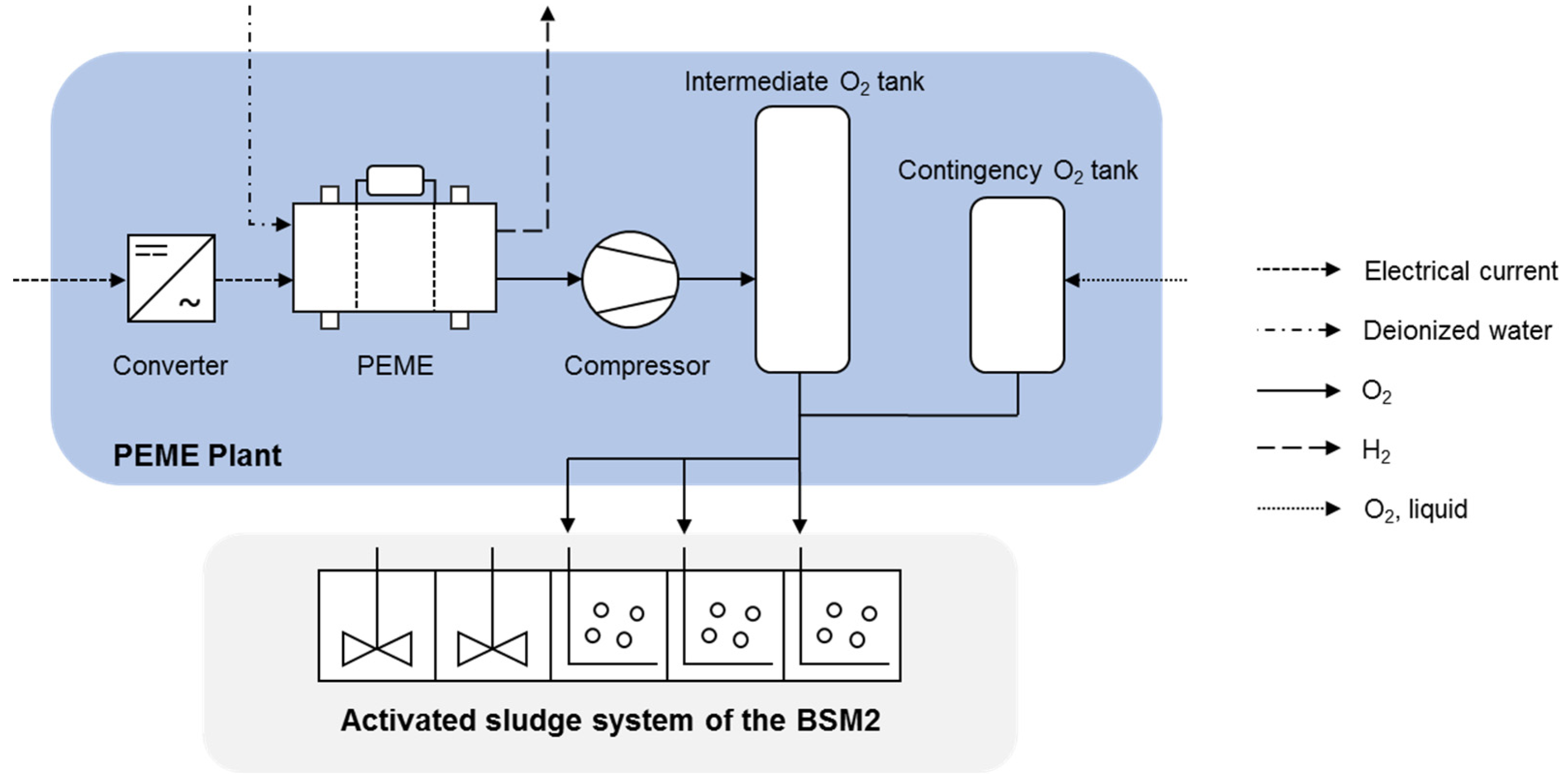
2.3. PEME Plant Model Implementation

The PEME plant model includes mathematical expressions for power consumption and mass balances of O₂, H₂, and deionized water. The PEME follows an operation cycle with a one-day period, alternating between full and minimal load. The number of hours at full load operation depends on the availability of electricity, which is location-dependent in the case of renewable sources. Two scenarios for the PEME plant operation and corresponding dimensions are analysed, where scenario 2 has a longer time in full load operation than scenario 1 (see

Table 1. Time at full load operation of the PEME plant for the analysed scenarios.

Scenario	Nominal % of Day at Full Load	Nominal Full Load Hours ${\mathit{t}}_{\mathit{F}\mathit{L}\mathit{H},\mathit{n}\mathit{o}\mathit{m}}$ (h·a−1)
1	40	3504
2	75	6750

). The values selected for the duration of full load operation are within the range of the scenarios reviewed in [23] and are meant to represent average and optimal electricity availability. An interlock is implemented in both scenarios to avoid breaching defined maximum ($p_{max}$ of 15 bar) and minimum ($p_{min}$ of 1.5 bar) overpressures in the intermediate O₂ tank. If the pressure in the intermediate tank approaches the defined limits (values above 14 bar or below 2.5 bar), the PEME switches to minimal or full load operation regardless of the predefined cycle.

The PEME stack is assumed to operate in a low-pressure range, and the produced gases are extracted at atmospheric pressure. At full load, the input current density $J$ is assumed to be 2.0 A·cm⁻², at a minimum of 0.4 A·cm⁻². The PEME cells have a total active area $a_c$ of 1250 cm². The power of the PEME ($P_{PEME}$) can then be calculated as:

$$P_{PEME}=J·a_c·{\phi }_{EZ}$$

(4)

where ${\phi }_{EZ}$ is the voltage of the electrolyser cells, which in turn depends on the input current density. Values for ${\phi }_{EZ}$ of 1.9 V at full load and 1.6 V at minimum load have been selected based on the compilation of PEME polarization curves presented in [24].

Since the starting times of PEMEs are usually below 15 min [16,25], changes in stack temperature and their effect on polarization curves during the start-up are neglected in the simulations. The gas and water flowrates have been calculated following the approach proposed in [15]. The molar flowrates of O₂, H₂, and deionized water in the electrolysis process are modelled using Faraday’s law:

$${\dot{n}}_{O_2,nom}^{EZ}=\frac{n_c·J·a_c}{4·F}·{\eta }_f$$

(5)

$${\dot{n}}_{H_2,nom}^{EZ}=\frac{n_c·J·a_c}{2·F}·{\eta }_f$$

(6)

$${\dot{n}}_{H_{2}O}^{EZ}=1.25·\frac{n_c·J·a_c}{2·F}·{\eta }_f$$

(7)

where ${\dot{n}}_{O_2,nom}^{EZ}$, ${\dot{n}}_{H_2,nom}^{EZ}$, and ${\dot{n}}_{H_{2}O}^{EZ}$ are nominal produced O₂, nominal produced H₂, and consumed deionized water, respectively. Furthermore, $n_c$ is the number of electrolytic cells connected in the series, $F$ is Faradays constant, and ${\eta }_f$ is the faradaic efficiency (above 99% for water electrolysis). The effective H₂ and O₂ molar flowrates supplied by the PEME are then calculated by introducing the efficiency factor ${\eta }_p$, taken here as a constant equal to 75%, to account for losses during drying and purification steps after the cells:

$${\dot{n}}_{O_2,eff}^{EZ}={\dot{n}}_{O_2,nom}^{EZ}·{\eta }_p$$

(8)

$${\dot{n}}_{H_2,eff}^{EZ}={\dot{n}}_{H_2,nom}^{EZ}·{\eta }_p$$

(9)

The intermediate storage tank and the compressor are modelled following the approach described in [26]. The change in pressure in the intermediate storage tank, assuming ideal gas behaviour, can be expressed as:

$$\frac{d{p}_{sto}}{dt}=\frac{T_{sto}·R}{V_{sto}}·({\dot{n}}_{O_2,eff}^{EZ}-{\dot{n}}_{O_2,eff}^{AS})$$

(10)

where $p_{sto}$, $T_{sto}$, and $V_{sto}$ are the pressure, temperature, and volume of the tank. $T_{sto}$ is ideally controlled at 25 °C. The flow of O₂ gas from the intermediate storage tank in the PEME plant to the AS system is assumed to show ideal behaviour, and no further components (e.g., operation of valves) have been considered. The power consumption of the compressor $P_{comp}$, assumed here to be a centrifugal compressor, can be expressed as Equation (11):

$$P_{comp}=\frac{{\dot{n}}_{O_2,eff}^{EZ}}{{\eta }_{comp}}·\frac{\kappa ·R·T_{PEME}}{\kappa -1}·\frac{{p_{sto}}^{\frac{\kappa -1}{\kappa }}}{p_{PEME}}$$

(11)

where ${\eta }_{comp}$ is the compressor efficiency (63%), $\kappa$ is the polytropic exponent (1.62), $T_{PEME}$ is the temperature of the PEME (ideally controlled at 80 °C), and $p_{PEME}$ is the pressure of the PEME, taken here as atmospheric pressure.

The behaviour of the contingency O₂ storage tank is not modelled. The required flowrate of external O₂ (${\dot{n}}_{O_2,ext}$) is equal to the demand of the AS system during the periods where the pressure in the intermediate tank is below the defined limit $p_{min}$:

$${\dot{n}}_{O_2,ext}=\left\{\begin{array}{c}{p}_{sto}>p_{min},\hspace{1em}\hspace{1em}0\hfill \\ p_{sto}\le p_{min},\hspace{1em}\hspace{1em}{\dot{n}}_{O_2,eff}^{AS}\end{array}\right.$$

(12)

The required contingency storage volume ($V_{cont}$) is then calculated based on the integral of ${\dot{n}}_{O_2,ext}$ over the simulation period. In a similar way, the behaviour of the AC/DC converter (transients and efficiency) is not modelled, and its capacity is assumed to be equal to the full load power of the PEME stack.

2.4. Techno-Economic Assessment

The TEA performed in this study considers the installation and operation of the PEME plant at the site of the conceptual BSM2 WWTP. The goal of the TEA is to gain insights on the development of the economics for the use of electrolysis O₂ in AS systems. For this, estimates of the net cost of production (from here on, $C_{NCP}$) of electrolysis O₂ are retrieved for PEME plants dimensioned according to the scenarios described in Table 1 and operating under different economic conditions. The obtained $C_{NCP}$ values are then compared with those corresponding to O₂ produced in conventional industrial processes (e.g., in cryogenic air separation units). The presented TEA focuses on the implementation of the PEME plant, which means that the costs related to modifications in the design and operation of the WWTP (e.g., modifications to gas injection systems in AS tanks) are outside the scope of this investigation.

2.4.1. Cost Estimation Framework

The cost estimation framework for chemical industries described in [27] has been used as a reference for the calculation of $C_{NCP}$ in the present study. $C_{NCP}$ are derived based on the apparent capital ($C_{CAPEX}$) and operational expenditures ($C_{OPEX}$) attributed to the system components and operation. Capital expenditures are calculated using the factorial method. As a first step, the investment costs of the main pieces of equipment or purchased equipment costs ($C_{PEC}$) are estimated. The $C_{PEC}$ include the costs of all components of the PEME plant model. The costs for the PEME stack, AC/DC converter, and compressor ($C_i$) are calculated using the capacity method as described in Equation (13) [27]:

$$C_i=C_{i,base}{·\left(\frac{S_i}{S_{i,base}}\right)}^{{\delta }_i}·\left(\frac{CEPCI}{{CEPCI}_{base}}\right)$$

(13)

where $C_{i,base}$ is the reference cost for an equipment unit $i$ with a size or capacity $S_{i,base}$, $S_i$ is the actual size or capacity of the equipment to be purchased, and ${\delta }_i$ is a reference empirical scaling exponent. The second term in Equation (13) accounts for historical changes in component costs. The Chemical Engineering Plant Cost Index (CEPCI) [28] is used here for historical cost scaling. The ${CEPCI}_{base}$ is the value of the index for the year of publication of $C_{i,base}$ and $CEPCI$ is the value for the year of estimation. The reference values used for $C_{i,base}$, $S_{i,base}$, and ${\delta }_i$ can be found in

Table 2. Data used for the cost estimation for PEME stacks, the AC/DC converters, and compressors following the capacity method.

Equipment Item	${\mathit{C}}_{\mathit{i},\mathit{b}\mathit{a}\mathit{s}\mathit{e}}$ (€)	${\mathit{S}}_{\mathit{i},\mathit{b}\mathit{a}\mathit{s}\mathit{e}}$ (kW)	${\mathit{\delta }}_{\mathit{i}}$ (-)	Reference	Year of Publication
PEME stack	1000 a	1	1	[3,30]	2020
AC/DC converter	160	1	1	[31,32]	2012
Compressor	267,000	445	0.67	[32,33]	2012

^a Varies according to the value of PEME stack costs $C_{PEME}$ in cost inventory (see Section 2.4.2).

, together with the year of publication of $C_{i,base}$. The corresponding values for ${CEPCI}_{base}$ and $CEPCI$ can be consulted under [29].

The costs for the intermediate and contingency O₂ storage tanks for the AS ($C_{T,i}$) are calculated using a component-specific capacity method expression as:

$$C_{T,i}=n_{T,i}·\left(a_{T,i}+b_{T,i}·S_{T,i}^{{\delta }_{T,i}}\right)·\left(\frac{CEPCI}{{CEPCI}_{base}}\right)$$

(14)

where $n_{T,i}$ is the number of tanks required to cover the designed volume. The corresponding values for the factors $a_{T,i}$, $b_{T,i}$, ${\delta }_{T,i}$, and the tank capacity $S_{T,i}$ can be found in

Table 3. Data used for the cost estimation of the O₂ tanks following the capacity method.

Equipment Item	${\mathit{a}}_{\mathit{T},\mathit{i}}$ ($)	${\mathit{b}}_{\mathit{T},\mathit{i}}$ ($·kg−1)	${\mathit{S}}_{\mathit{T},\mathit{i}}$ (kg)	${\mathit{\delta }}_{\mathit{T},\mathit{i}}$ (-)	Reference	Year of Publication
Intermediate O2 tank	12,800	73	7800	0.85	[27,34]	2010
Contingency O2 tank	17,400	79	900	0.85	[27,34]	2010

.

The total purchased equipment costs ($C_{PEC}$) are determined as follows:

$$C_{PEC}=\sum C_i+\sum C_{T,i}$$

(15)

The obtained $C_{PEC}$ are used to estimate the remaining cost items of $C_{CAPEX}$. All involved $C_{CAPEX}$ cost items are estimated using the factorial approach based on the so-called Lang factors ($f_{CAPEX,i}$), which can be represented as an example of the case of ISBL costs ($C_{ISBL}$) as follows:

$$C_{ISBL}=\underset{\begin{array}{c}Cost basis\\ \left(C_{CAPEX,i}\right)\end{array}}{\underbrace{C_{PEC}}}\sum _{i=1}^n{f}_{CAPEX,i}$$

(16)

Table 4. Capital expenditure $C_{CAPEX}$ estimation methodology via the factorial method and chosen cost items and Lang factors based on literature data taken from [27,34,35].

Superordinate Cost Item ${\displaystyle \sum _{\mathit{i}}}{\mathit{C}}_{\mathit{C}\mathit{A}\mathit{P}\mathit{E}\mathit{X},\mathit{i}}·{\mathit{f}}_{\mathit{C}\mathit{A}\mathit{P}\mathit{E}\mathit{X},\mathit{i}}$	CAPEX Cost Item Description $\mathbf{}{\mathit{C}}_{\mathit{C}\mathit{A}\mathit{P}\mathit{E}\mathit{X},\mathit{i}}·{\mathit{f}}_{\mathit{C}\mathit{A}\mathit{P}\mathit{E}\mathit{X},\mathit{i}}$	Cost Basis (€) ${\mathit{C}}_{\mathit{C}\mathit{A}\mathit{P}\mathit{E}\mathit{X},\mathit{i}}$	Index $\mathit{i}$	Lang Factor ${\mathit{f}}_{\mathit{C}\mathit{A}\mathit{P}\mathit{E}\mathit{X},\mathit{i}}$
Inside battery limits ($C_{ISBL}$)	Equipment purchase	$C_{PEC}$	1	1
	Equipment installation		2	0.3
	Piping (installed) (valves, fittings, pipes, supports, and labour)		3	0.3
	Instrumentation and controls (installation labour, auxiliary equipment)		4	0.3
	Electrical systems (installed) (wiring, lighting, transformation, and services)		5	0.1
Outside battery limits ($C_{OSBL}$)	Additions to site infrastructure Water, air and electricity supply nodes Piping, storage, and distribution	$C_{ISBL}$	6	0.1
Contingency charges ($C_{CC}$)	Compensation of cost estimates Price/currency fluctuations Contractor/labour disputes	$C_{ISBL}+C_{OSBL}$	7	0.2
Design and engineering ($C_{DE}$)	Engineering and supervision	$C_{ISBL}+C_{OSBL}$	8	0.3
	Construction expenses		9	0.3
	Contractor fee		10	0.1
Working capital ($C_{WC}$)	Feed/product/spare parts inventory Cash on hand	$C_{ISBL}+C_{OSBL}$	11	0.1
Start−up expenses ($C_{SE}$)	General start-up expenses	$C_{ISBL}+C_{OSBL}$	12	0.05

summarizes the employed Lang factors $f_{CAPEX,i}$ for all superordinate cost items ($C_{ISBL}$, $C_{OSBL}$, $C_{CC}$, $C_{DE}$, $C_{WC}$ and $C_{SE}$) that have been used in this study. Depending on the respective superordinate cost item, the different cost basis $C_{CAPEX,i}$ may be employed. Taking into account that the PEME plant is supposed to be installed at the site of an existing WWTP, cost items related to civil engineering and yard improvement required when a project is to be developed at a completely new site (so-called green field site) are not considered here.

After calculating all relevant cost items, the total capital expenditures $C_{CAPEX}$ can be determined based on the so-called fixed capital investments $C_{FCI}$, which represent the entirety of investment costs attributed to the planning/designing, construction, and erection of the plant, and the working capital $C_{WC}$ and start-up expenses $C_{SE}$, which account for the capital used to maintain the plant’s operation over its lifetime.

$$C_{CAPEX}=\underset{=C_{FCI}}{\underbrace{C_{ISBL}+C_{OSBL}+C_{CC}+C_{DE}}}+C_{WC}+C_{SE}$$

(17)

The operational costs $C_{OPEX}$ can be subdivided into variable costs of production $C_{VCP}$, fixed costs of production $C_{FCP}$, and by-product revenues $R_{H_2}$ from the sale of H₂:

$$C_{OPEX}=C_{VCP}+C_{FCP}-R_{H_2}$$

(18)

$C_{VCP}$ are operational costs directly related to the plant´s output and therefore change with the operation mode, e.g., full or minimal load. For the estimation of $C_{VCP}$, the expression in Equation (19) is used:

$$C_{VCP}=C_{H_{2}O}+C_{O_2,ext}+C_E+C_{R,PEME}$$

(19)

where $C_{H_{2}O}$ are the costs of the consumed deionized water, $C_{O_2,ext}$ are the costs of consumed liquid O₂ from the contingency tank, $C_E$ are the costs of electricity, and $C_{R,PEME}$ are the costs for the replacement of PEME stacks until the plants end of lifetime (EOL). The yearly consumption of deionized water, liquid O₂, and electricity is obtained from the simulation results and is assumed to be constant until plants reach EOL. The respective specific costs of deionized water $c_{H_{2}O}$, external liquid O₂ $c_{O_2,ext}$, and electricity $c_E$ are described in detail in Section 2.4.2.

The cost of PEME stack replacement $C_{R,PEME}$ is calculated based on the stack lifetime, plant lifetime, and cumulative full load operating hours. It is assumed that stack costs for each replacement are comprised of 50% of the initial specific PEME stack capital costs, as only the cells are replaced and the periphery and housing remain intact and are still usable.

Contrary to $C_{VCP}$, fixed costs of production $C_{FCP}$ are independent of the actual operation or output of the plant. For the calculation of $C_{FCP}$, a factorial estimation methodology has also been applied (see

Table 5. Fixed costs of production $C_{FCP}$ estimation methodology based on the factorial method and retrieved Lang factors from the literature according to [27].

Superordinate OPEX/FCP Cost Item ${\mathit{C}}_{\mathit{O}\mathit{P}\mathit{E}\mathit{X},\mathit{i}}·{\mathit{f}}_{\mathit{O}\mathit{P}\mathit{E}\mathit{X},\mathit{i}}$	Cost Basis (€) ${\mathit{C}}_{\mathit{O}\mathit{P}\mathit{E}\mathit{X},\mathit{i}}$	Index $\mathit{i}$	Lang Factor ${\mathit{f}}_{\mathit{O}\mathit{P}\mathit{E}\mathit{X},\mathit{i}}$
Supervision ( $C_{SV}$)	$C_{OL}$	1	0.25
Direct salary overhead ( $C_{DSO}$) (Non-salary costs: Health insurance and benefits)	$C_{OL}+C_{SV}$	2	0.4
Maintenance ($C_{MT}$)	$C_{ISBL}$	3	0.03
Property taxes and insurance ( $C_{PTI}$)	$C_{ISBL}$	4	0.01
Rent of land ( $C_{ROL}$)	$C_{ISBL}+C_{OSBL}$	5	0.01
Environmental charges ( $C_{EV}$)	$C_{ISBL}+C_{OSBL}$	6	0.01

and Equation (20)).

$$C_{FCP}=\underset{=C_{OL}}{\underbrace{c_{OL}·y_{PL}}}+\underset{\begin{array}{c}Capital charges\\ on WC/SE loan\end{array}}{\underbrace{\left(C_{WC}+C_{SE}\right)·i_d·y_{PL}}}+\sum _{i=1}^6{C}_{OPEX,i}·f_{OPEX,i}$$

(20)

The total operating labour costs $C_{OL}$ represent the costs for the personnel in charge of the plant and are calculated based on the specific operating labour costs $c_{OL}$, taken here as 60,000 €·a⁻¹, and the plant’s lifetime $y_{PL}$. Capital charges included within $C_{FCP}$ are attributed to the interest payments on the loan of working capital and start-up expenses, which are supposed to be entirely funded by debt. These capital charges are included within $C_{FCP}$, since the total working capital and total start-up expenses are recovered at the EOL of the plant, and hence the incurring interest payments must not be included in the estimation of $C_{CAPEX}$ via Equations (15) and (16) and Table 4 [27]. In Equation (20), $i_d$ is the interest rate of the capital charges on working capital and total start-up expenses loan, taken here as 0.05. As in the case of the cost items of $C_{CAPEX}$, the remaining items of $C_{FCP}$ are estimated based on the superordinate OPEX cost items $C_{OPEX,i}$ and their respective Lang factors $f_{OPEX,i}$, as indicated in Table 5.

By-product revenues ($R_{H_2}$) considered in this study correspond to the income generated by the sale of the produced H₂ during the PEME plant lifetime. In the same way as with the costs for deionized water, liquid O₂, and electricity, $R_{H_2}$ is calculated based on the simulation results for yearly H₂ production ($\sum {\dot{m}}_{H_2,eff}^{EZ}$) and the specific selling or market price $c_{H_2}$ (also see Section 2.4.2). The yearly amount of produced H₂ is also assumed to remain constant until the plants reach EOL.

In order to calculate the $C_{NCP}$ of electrolysis O₂, the annuity method based on the total spent fixed capital investment costs $C_{FCI}$ is applied. The total $C_{FCI}$ is annualized by determining the annual capital charge ($C_{ACC}$) required to fully reimburse the initial capital investment until the plants reach EOL. As a result, the fixed capital investments after interest ($C_{FCI,ai}$), also known as depreciation costs, are determined:

$$C_{FCI,ai}=\underset{\begin{array}{c}Annual capital\\ charge \left(C_{ACC}\right)\end{array}}{y_{PL}\underbrace{·C_{FCI}·\frac{i_c{\left(i_c+1\right)}^{y_{PL}}}{{\left(i_c+1\right)}^{y_{PL}}-1}}}$$

(21)

The FCI are financed by debt and equity represented by a compound interest rate $i_c$ (also weighted average cost of capital; see Equation (22)) with respective interest rates for debt $i_d$ and equity $i_e$, as well as a specific debt ratio $r_d$ for both capital sources. In the present studies, $i_e$ is taken as 0.1 and $r_d$ as 0.5, resulting in an $i_c$ value of 0.075.

$$i_c=r_d·i_d+\left(1-r_d\right)·i_e$$

(22)

Based on the retrieved values of $C_{FCI,ai}$ and $C_{OPEX}$, as well as potential revenues ($R_S$) from plant salvage (PEME stacks) at plant EOL and the cumulative annual O₂ production ($\sum {\dot{m}}_{O_2,eff}^{EZ}$), the net costs of O₂ production ($C_{NCP}$) are determined (Equation (23)).

$$C_{NCP}=\frac{C_{FCI,ai}+C_{OPEX}-R_S}{y_{PL}·\sum {\dot{m}}_{O_2,eff}^{EZ}}$$

(23)

The chosen annuity approach assumes that investments and cash flows start immediately and, due to the integral nature of this approach, no specific timing of investments and revenues has been considered. Moreover, taxes and depreciation charges have been neglected in the annuity approach and hence the determination of $C_{NCP}$. Revenues from PEME stack salvage are only considered if the remaining lifetime of the installed PEME stack at EOL is larger than 8000 h. The salvage value is derived from the initial stack investment costs, the ratio of the remaining and initial stack lifetime $(y_{PEME}$), as well as an additional salvage factor of 0.5.

In addition to the annuity method, the potential specific minimum selling price of O₂ through the PEME plant ($c_{MSP,O_2}$) is calculated via a cash flow analysis, i.e., determination of the net present value (NPV) at the plant EOL. With the annual gross profit ($P_n$), the depreciation tax allowances ($D_n$), and the corporate tax rate ($t_{cp}$), the annual cash flow (${CF}_n$) in each year $n$ can be assessed (Equations (24) and (25)). Subsequently, the NPV is calculated based on Equation (26). To comply with the initial assumption of an NPV of zero at the plant’s EOL, $c_{MSP,O_2}$ is varied via a simple search algorithm until the condition formulated in Equation (26) is reached.

$$P_n=c_{MSP,O_2}·\sum {\dot{m}}_{O_2,eff}^{EZ}+c_{H_2}·\sum {\dot{m}}_{H_2,eff}^{EZ}+\frac{R_S-C_{VCP}-C_{FCP}}{y_{PL}}$$

(24)

$${CF}_n=P_n·\left(1-t_{cp}\right)+D_n·t_{cp}$$

(25)

$$NPV=\sum _{n=1}^{y_{PL}}\frac{{CF}_n}{{(1+i_c)}^n}=0$$

(26)

A straight-line depreciation over 10 years and a corporate tax rate ($t_{cp}$) of 0.3 are assumed. All capital expenses are spent in year zero. The TEA studies are carried out within the software framework of MATLAB R2017b.

2.4.2. Cost Inventory and Market Analysis

To provide economic data for the calculations described in Section 2.4.1 and allow for the realization of the TEA under various conditions, a cost inventory for the items with significant impact on the economic performance of the PEME plant has been defined. The items selected for the cost inventory include the following:

• Electricity price (LCOE) depending on the source of origin.
• Selling price of produced H₂ depending on market conditions.
• Price of O₂ from conventional sources.
• The investment and replacement costs attributed to the PEME.

The presented TEA is performed for the reference year 2020 based on current data and also for 2030 based on forecasts presented in literature to reflect the development of the process’s economics. Three different sets of economic parameters have been defined for each of the selected years in order to represent optimistic, neutral, and pessimistic economic conditions for the project’s implementation. Four different electricity sources have been considered in the present study, namely conventional, PV, and wind (off-shore and on-shore) energy plants. The costs defined for the different items in the cost inventory, as well as the PEME stack lifetime $y_{PEME}$, are presented in

Table 6. Cost inventory for the estimation of net costs of production (NCP) for electrolysis O₂ based on reference values taken from literature [36,37,38,39,40,41,42].

		2020			2030
		Optimistic	Neutral	Pessimistic	Optimistic	Neutral	Pessimistic
LCOE $c_E$ (€·MWh−1)	Conventional	31	43	55	47	71	94
	PV	31	57	140	21	51	81
	Wind on shore	39	61	83	25	53	81
	Wind off shore	72	105	138	56	78	101
H2 price $c_{H_2}$ (€·kg−1)		6	5	4	4	3	2
PEME stack lifetime $y_{PEME}$ (h)		67,500	59,000	50,500	85,000	75,500	66,125
PEME stack cost $c_{PEME}$ (€·kW−1)		867	1000	1225	453	600	780
O2 price $c_{O_2,ext}$ (€·t−1)		100	100	100	134 a	122 b	110 c

^a annual price increase of 3%, ^b annual price increase of 2%, ^c annual price increase of 1%.

. For 2020, the plant’s lifetime $y_{PL}$ is assumed to be 20 years, while for 2030, it is assumed to be 30 years.

The projections of the cost inventory reflect the trends reported in the literature [36,37,38,39,40,41,42]. While electricity prices for all renewable sources are expected to decrease, the price for conventional sources is expected to increase due to higher costs for CO₂ emission certificates. Improvements in electrolyser performance and the corresponding decrease in investments are expected to result in decreasing H₂ selling prices in 2030. It is important to point out that, although a stronger reduction in H₂ production costs would be a positive trend regarding the transition to a sustainable energy system, this would increase the calculated NCP for O₂, and therefore the pessimistic scenario considers lower H₂ selling prices. Conventional O₂ prices are assumed to increase at a different rate for each economic condition. The cost of deionized water $c_{H_{2}O}$ is also assumed to increase with time, taking a value of 2 €·m⁻³ and 3 €·m⁻³ in 2020 and 2030, respectively.

3. Results and Discussion

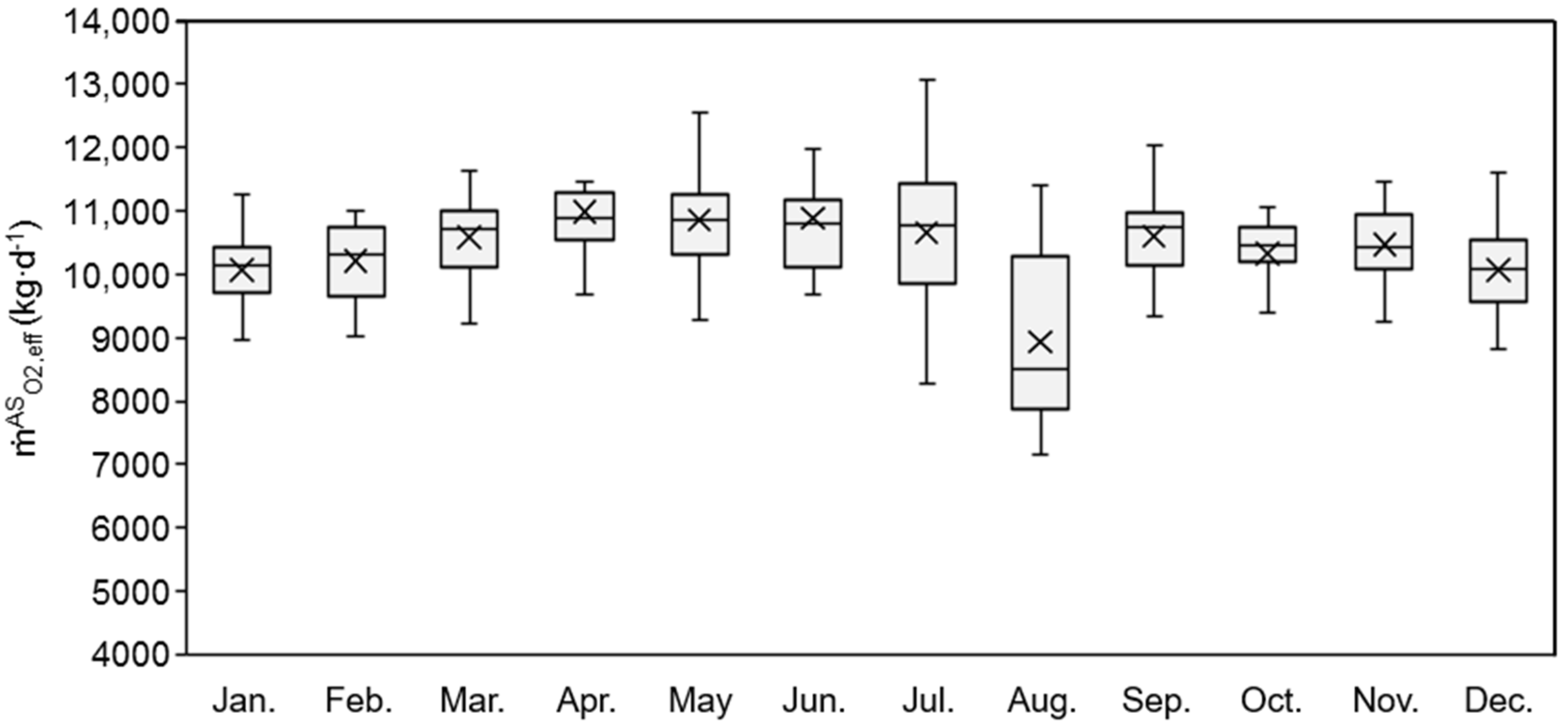
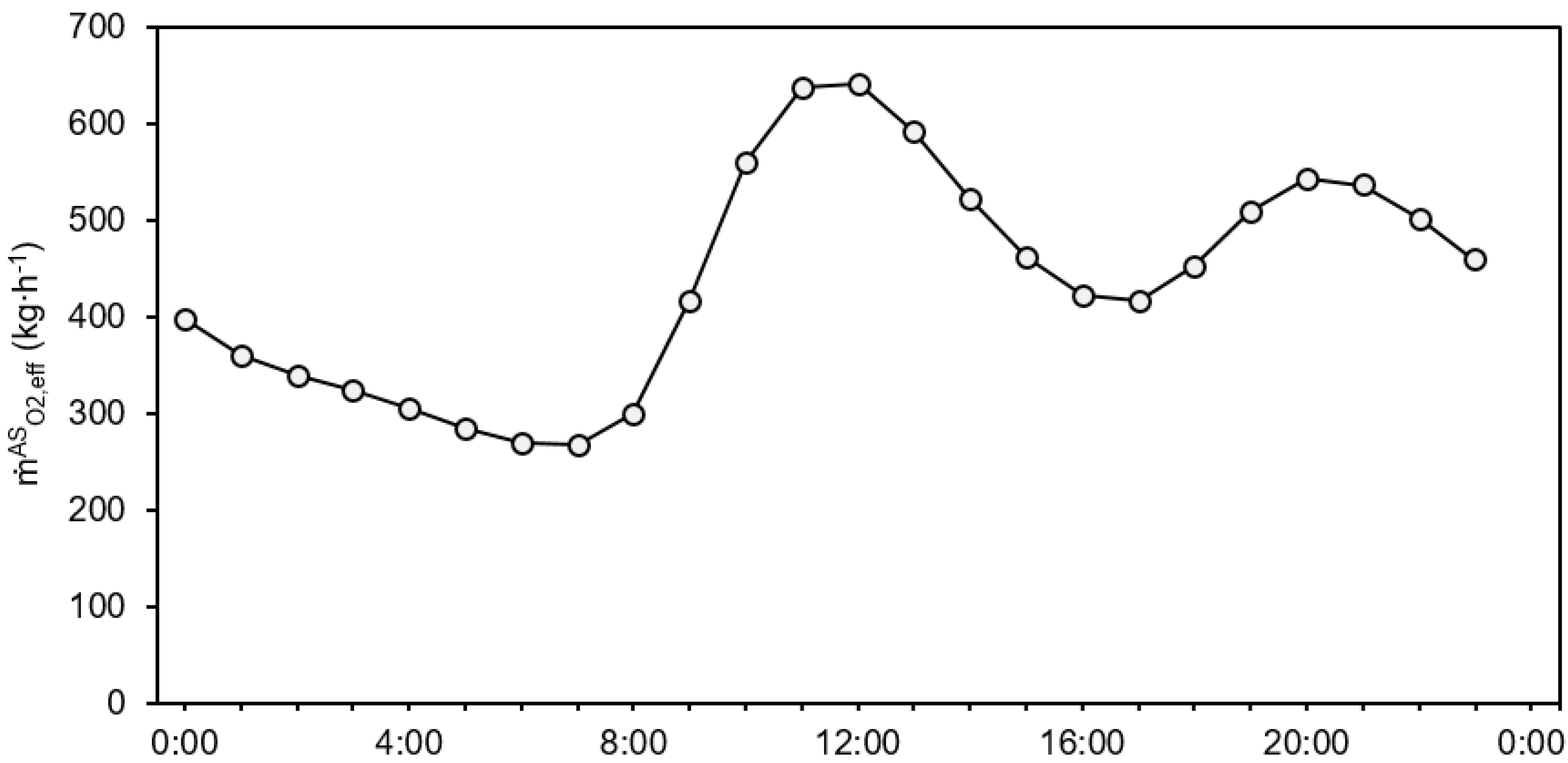
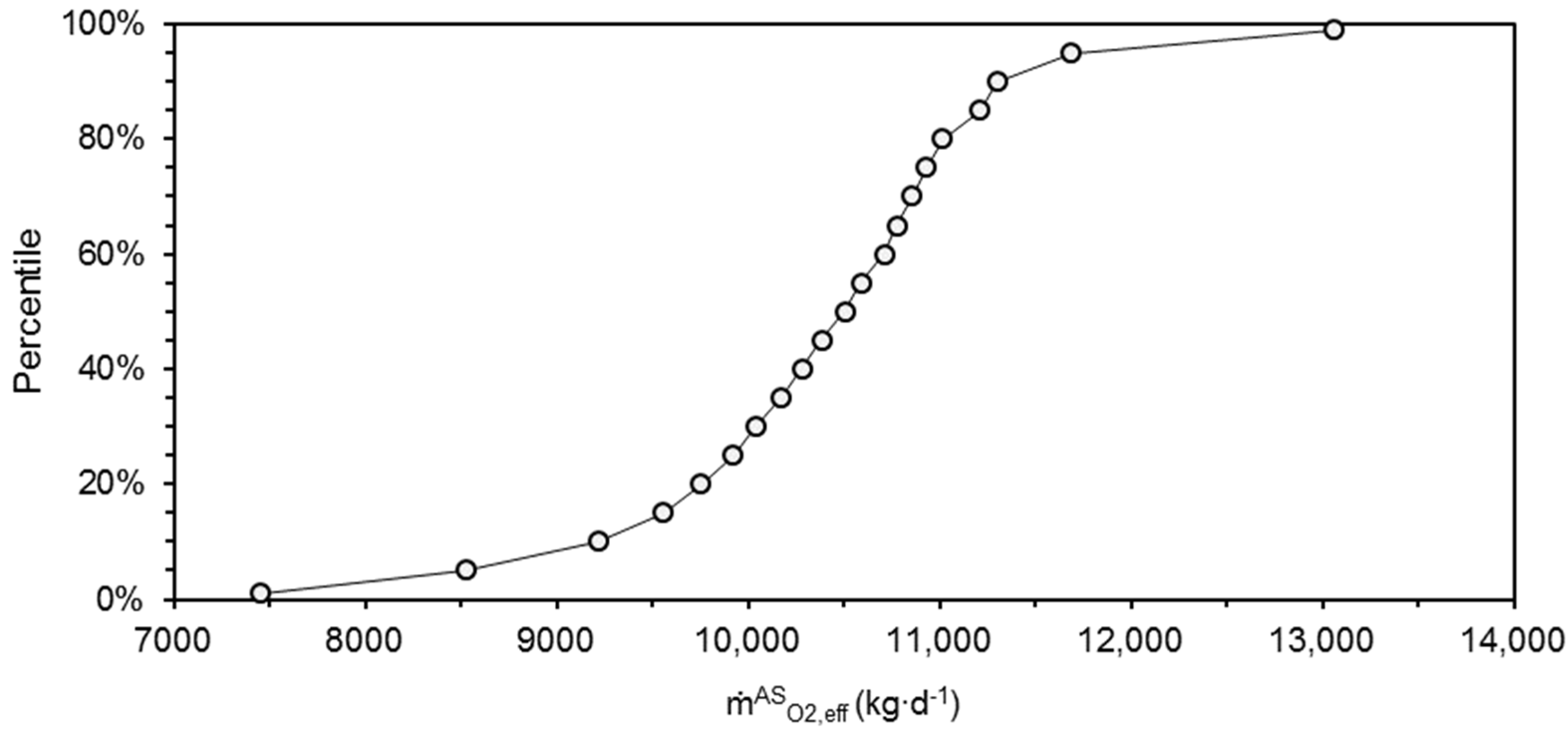
3.1. O₂ Demand of the BSM2 WWTP

The behaviour of the O₂ demand of the AS system in the BSM2 can be seen in Figure 2 after converting ${\dot{n}}_{O_2,eff}^{AS}$ to kg·d⁻¹ (${\dot{m}}_{O_2,eff}^{AS}$). The average daily O₂ demand for the BSM2 was calculated at 10,388 kg·d⁻¹. The use of larger ${DO}_{sat}$ values to account for the use of pure O₂ (see Section 2.2.) results in higher transfer rates $OTR$ for a given $k_{L}a$ and measured $DO$ concentration when compared with air (see Equation (1)). The $k_{L}a$ values calculated by the PI controller are therefore lower in this study than in the original BSM2, i.e., less gas volume and therefore less energy for gas injection is required when using pure O₂. When $k_{L}a$ values are too low, the additional mixing energy for maintaining the sludge in suspension in the nitrification tanks is to be calculated as part of the operational costs in the BSM2 [18]. However, since the TEA scope includes only the PEME plant, these effects of pure O₂ use on the operational costs of WWTP are not further assessed.

The effect of seasonal changes can be seen in higher O₂ demand during warmer months, which can be explained by the decrease in ${DO}_{sat}$ at higher temperatures and the corresponding decrease in the amount of O₂ that can be maintained in the water phase. A further seasonal effect that can be seen in Figure 2 is the decrease in O₂ demand caused by less household wastewater production during the summer holiday season [19]. Intraday variations in O₂ demand follow the profile of wastewater inflow into the WWTP, i.e., are higher during daytime with peaks around midday and in the evening (see Figure 3).

The cumulative histogram for ${\dot{m}}_{O_2,eff}^{AS}$ can be seen in Figure 4, showing that during 80% of the simulation time, the O₂ demand is between approx. 9200 and 11,300 kg·d⁻¹.

3.2. Dimensioning of PEME Plant

The selected capacities of the PEME plant components for each scenario and the corresponding simulation results are shown in

Table 7. Result of the dimensioning of the PEME plant for both scenarios.

Parameter	Scenario 1	Scenario 2
$n_c$ (-)	1350	1000
$P_{PEME}$ (kW)	6400	4750
$P_{comp}$ (kW)	37	27
$V_{sto}$ (m3)	250	200
$V_{cont}$ (m3)	5	28
Effective % of time at full load	47	72
$t_{FLH,eff}$ (h·a−1)	4073	6259
$\sum {\dot{m}}_{O_2,eff}$ (t·a−1)	3782	3780
$\sum {\dot{m}}_{H_2,eff}$ (t·a−1)	476	476
Time with $p_{sto}$ < $p_{min}$ (d·a−1)	0.4	2.5
Time with $p_{sto}$ > $p_{max}$ (d·a−1)	0	0

. The operation cycles defined in Section 2.3 are subject to changes due to the activation of the interlock, resulting in an effective amount of hours at full load $t_{FLH,eff}$ that differs from the $t_{FLH,nom}$ presented in Table 1. When analysing gas production, it can be seen that the difference in PEME capacity between both scenarios is compensated by the difference in $t_{FLH,real}$, resulting in a very similar production of H₂ and O₂. In both scenarios, there are periods where, despite the activation of the interlock, the O₂ flowrate produced by the PEME at full load capacity is under the O₂ demand, resulting in $p_{sto}$ values below $p_{min}$ and the need to supply O₂ from the contingency tank. The higher PEME capacity and storage tank volume in scenario 1 results in a significantly shorter period with $p_{sto}$ below $p_{min}$ when compared with scenario 2, leading to a larger volume of the contingency tank in scenario 2. These critical periods are, however, relatively short; in both scenarios, the PEME plant is capable of supplying enough O₂ to the BSM2 WWTP during more than 99% of the simulated time without recurring to the contingency tank. For neither of the scenarios is there a period where $p_{sto}$ is above $p_{max}$.

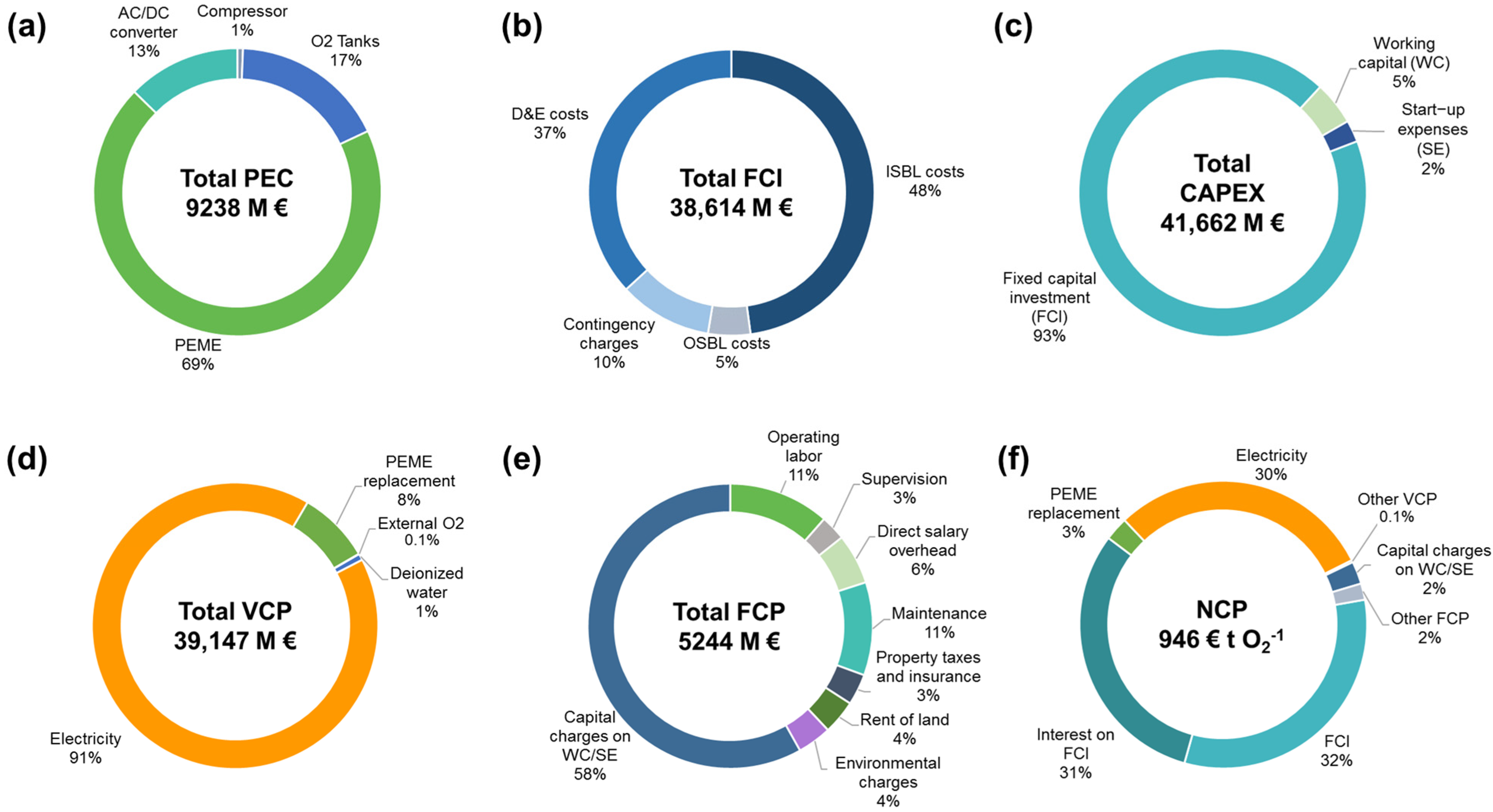
3.3. Economic Assessment

The cost breakdown of all relevant cost categories of purchased equipment costs $C_{PEC}$, total capital expenses $C_{CAPEX}$, operational costs $C_{OPEX}$, as well as the net O₂ production costs $C_{NCP}$ are presented in Figure 5 for an exemplary case (scenario 1 in 2020, under neutral economic conditions and supplied with PV electricity). The breakdowns shown in Figure 5a to 5e are representative for all other assessed cases, i.e., the proportion of cost items is similar. In all cases, $C_{PEC}$ is dominated by the initial PEME investment cost (between 53.2% and 73.4% of $C_{PEC}$ for scenario 1 and between 50.7% and 71.5% for scenario 2), followed by the investments for O₂ tanks, the converter, and the compressor. The share of $C_{PEC}$ made up by PEME investment costs is between 13.2% and 7.5% lower in 2030 than in 2020 due to the assumed decrease in the PEME stack price. $C_{FCI}$, which make up 92.7% of $C_{CAPEX}$, are dominated by investments inside battery limits $C_{ISBL}$ (47.8%) and the costs of design and engineering $C_{DE}$ (36.8%).

The costs of electricity consistently make up more than 85% of $C_{VCP}$. The cost share of PEME stack replacement in $C_{VCP}$ is always below 10%, while the sum of the shares of deionized water and external O₂ for the contingency tank is always below 3%. Capital charges on working capital and total start-up expenses make up the majority of the fixed costs of production $C_{FCP}$ (between 50 and 59.8%).

An overview of all calculated $C_{NCP}$ after revenues are presented in

Table 8. Calculated net costs of production $C_{NCP}$ in €·t⁻¹.

Year	Scenario	Electricity Source	Optimistic	Neutral	Pessimistic
2020	Scenario 1	Conventional	500	830	1232
		PV	500	945	1935
		Wind on shore	566	978	1464
		Wind off shore	839	1342	1919
	Scenario 2	Conventional	286	609	977
		PV	286	727	1693
		Wind on shore	353	761	1212
		Wind off shore	631	1131	1676
2030	Scenario 1	Conventional	452	874	1311
		PV	237	709	1203
		Wind on shore	270	725	1203
		Wind off shore	526	932	1369
	Scenario 2	Conventional	347	751	1165
		PV	128	582	1055
		Wind on shore	161	599	1055
		Wind off shore	423	810	1224

. Lower investment costs for the PEME stacks result in overall lower $C_{NCP}$ for scenario 2. In 2020, all calculated $C_{NCP}$ are higher than the price of O₂ from conventional sources (100 €·t⁻¹).

In 2030 and under positive economic conditions, competitive production costs below or near the conventional O₂ price (134 €·t⁻¹) are achieved for the PEME plant designed according to scenario 2 and supplied by PV (128 €·t⁻¹) and wind on-shore electricity (161 €·t⁻¹). Such relatively low $C_{NCP}$ are the result of optimistic trends regarding costs of PEME stacks and renewable electricity supply.

As can be seen in Figure 5f, $C_{NCP}$ are dominated by fixed costs of investments, the interest on these investments, and electricity costs. However, the share of electricity costs in $C_{NCP}$ varies greatly among the analysed cases (between 20.2 and 51.5% in scenario 1 and between 25 and 57.6% in scenario 2). In 2020, the difference between optimistic and pessimistic PV electricity costs is largest among all energy sources considered (see Table 6). For this reason, both the highest and lowest C_NCP values in 2020 correspond to the PV electricity supply. In 2030, the costs of PV and wind on-shore electricity are very similar, with PV resulting in slightly lower $C_{NCP}$, while more expensive conventional and wind off-shore electricity supply results in higher production costs. The sum of all cost items aside from electricity, $C_{FCI}$, and interests on $C_{FCI}$ consistently make up less than 10% of $C_{NCP}$.

It is important to consider that items in the cost inventory were all assigned either optimistic, neutral, or pessimistic values in each case (see Table 6); thus, the results presented in Table 8 do not include combinations of economic conditions. For example, if optimistic values are selected for the cost of PV electricity and the selling price of H₂ in 2030 while pessimistic values are kept for all other items in the cost inventory, the resulting C_NCP for scenario 2 would be 296 €·t⁻¹ rather than 1055 €·t⁻¹.

The maximum and minimum calculated potential O₂ selling prices $c_{MSP,O_2}$ are shown in

Table 9. Range of calculated minimum selling prices $c_{MSP,O_2}$ in €·t⁻¹.

	Scenario 1		Scenario 2
	2020	2030	2020	2030
$c_{MSP,O_2}$ max.	2184	1525	1882	1343
$c_{MSP,O_2}$ min.	695	350	436	215

. Values for $c_{MSP,O_2}$ are always higher than $C_{NCP}$ since plant depreciation and tax on income are included in their calculation (see Equation (24)). The obtained selling prices are therefore not competitive with conventional O₂ sources with prices of 100 €·t⁻¹ (2020) and 134 €·t⁻¹ (2030) in any of the studied cases.

3.4. Further Research

The present study offers a methodology for the analysis of the economics of O₂ valorisation in biological treatment steps of WWTPs based on a recognized benchmark such as the BSM2 and simple models for the components of a PEME plant. Regarding possible subjects for further investigations, in this study both the efficiency factor used to represent O₂ losses in gas separation steps ${\eta }_p$ and the $OTE$ of the oxygenation system installed at the WWTP are taken as constant. New developments in gas separation units and oxygenation systems are expected to lead to higher efficiencies [43,44], which in turn would help to reduce $C_{NCP}$. Furthermore, many of the AS systems using pure O₂ are designed with a closed headspace to enable the collection and reuse of injected O₂ [12], which would result in lower electrolyser capacities being required. Future TEAs could address a closed AS system, however additional effects of closed headspace design such as the inhibition of nitrification processes due to CO₂ accumulation and pH decrease should also be considered [12,45,46]. The costs for the adaption of the WWTP infrastructure to the use of pure O₂ should also be analysed.

Further effects of pure O₂ in biological and chemical processes in AS systems are outside the scope of this study. These include benefits such as reduction in sludge production, reduction in fouling foaming and improvements in treatment efficiency [12,13]. Such effects of the use of pure O₂ from electrolysers in AS systems should therefore also be investigated experimentally. Possible synergies between electrolyser plants and other processes in WWTPs can be considered in future simulation studies. These may include the use of heat recovered from the electrolysers cells or the methanation of biogas produced in sludge treatment with the H₂ from the electrolyser [10].

The dimensioning of the PEME plant was done to cover the whole O₂ demand from the BSM2 WWTP with a capacity of 80,000 PE. In Germany this correspond to the second largest category for WWTP capacity defined by the national environment agency. More than 60% of wastewater in Germany is treated at WWTPs with installed capacities above 10,000 PE, although these larger plants make less than 10% of the total number of WWTPs [47]. The proposed methodology can be applied to analyse the economics of similar projects to fully supply smaller WWTPs or partially cover the O₂ demand in larger ones (e.g., pre-treatment step with pure O₂ before conventional AS system supplied with air). A rough estimation of the required PEME capacity for a smaller WWTP of 10,000 PE treating wastewater with a typical O₂ demand of 1200 kg O₂·d⁻¹ [48] can be done by a lineal extrapolation of the PEME capacities presented in Section 3.2. This results in a required capacity of around 740 kW for scenario 1 and 550 kW for scenario 2. The use of pure O₂ is recommended for the treatment of highly-strength wastewater [12], thus future analyses should be done by using models of industrial WWTPs. The same is true for membrane bioreactors (MBR), for which the use of pure O₂ has been shown to increase treatment efficiency and reduce membrane fouling [49].

Regarding the analysed economic conditions, further investigations could integrate changes in electricity prices during the simulated period. In future renewable-based electricity networks, the operation of electrolysers can be adjusted through demand side management according to prices and availability of energy [16]. Within a flexible electricity pricing scheme, plants operators could benefit from reduced electricity costs by adjusting the operation scheme of the PEME accordingly while at the same time providing network regulation services. Moreover, analyses in this study do not consider variations in the cost inventory during the plants lifetime; the prices and performance of the PEME plant are assumed constant until EOL for simplification. More detailed consideration of the H₂ valorisation processes should also be included in future studies (e.g., variations in sold amount and price or the implementation of internal valorisation measures).

4. Conclusions

Power-to-gas technologies based on water electrolysis are expected to play a central role in future renewable energy networks, where green H₂ and derived synthetic fuels are used as alternatives to fossil fuels. In the electrolysis process, large amounts of O₂ are produced alongside H₂, however O₂ is usually seen as a by-product and discarded into the atmosphere. In the present study the economics of the valorisation of electrolysis O₂ in biological treatment steps of municipal WWTPs has been analysed based on the results of mathematical simulation models.

The operation WWTP of the BSM2 has been modelled alongside a PEME system and used to simulate O₂ supply for an operation period of one year. Two scenarios regarding full load hours per year and corresponding PEME plant dimensions have been considered. Simulation data on the amount of consumables required and the produced gas flowrates was used as an input for a TEA on the net costs of O₂ production NCP, assuming that the produced H₂ is sold to a nearby industry. The TEA was performed for the years 2020 and 2030 under sets of optimistic, neutral and pessimistic conditions regarding costs and revenue streams.

Simulation results show that for 80% of the simulation period the O₂ demand of the AS of the BSM2 plant is between approx. 9200 and 11,300 kg·d⁻¹. The dimensions of the PEME stack and amount of full load hours were 6.4 MW and 4073 h·a⁻¹ for scenario 1, whereas 4.8 MW and 6259 h·a⁻¹ for scenario 2. The PEME plants in both scenarios were able to cover the O₂ demand for more than 99% of the simulated time without having to rely on contingency O₂ storage. The results of the TEA show that NCP are dominated by the investment and respective interests on the PEME stacks, as well as the electricity costs. The sum of other cost components makes less than 10% of the NCP. Although for the year 2020 NCP for O₂ produced by the PEME plant are higher than references for the costs of industrial O₂, in 2030 the combination of lower investment costs for PEME stacks and lower renewable electricity prices (PV and wind on shore) resulted in competitive electrolysis O₂ costs when assuming optimistic economic conditions.

Further studies can follow the approach described here to analyse the economics of electrolysis O₂ supply to conventional WWTPs of different size or different systems such as MBRs. The simple models for the PEME plant and the O₂ supply process described here should also be expanded to include the effects of using pure O₂ in AS system, more detailed considerations regarding H₂ valorisation, as well as changes in electricity prices and system performance during the plants lifetime. The use of electrolysers at WWTPs for demand side management by adjusting the operation according to the energy networks behaviour should also complement the presented results.

References

1. Staffell, I.; Pfenninger, S. The increasing impact of weather on electricity supply and demand. Energy 2018, 145, 65–78. [Google Scholar] [CrossRef]
2. Kanellopoulos, K.; Blanco, H. The potential role of H2 production in a sustainable future power system—An analysis with METIS of a decarbonised system powered by renewables in 2050. Eur. Comm. JRC Tech. Rep. 2019, 10, 540707. [Google Scholar] [CrossRef]
3. Glenk, G.; Reichelstein, S. Economics of converting renewable power to hydrogen. Nat. Energy 2019, 4, 216–222. [Google Scholar] [CrossRef] [Green Version]
4. BMU Nationale Wasserstrategie—Entwurf des Bundesumweltministeriums. Bonn, 2021. Available online: www.bmu.de (accessed on 28 October 2021).
5. IRENA. Green Hydrogen Cost Reduction—Scaling Up Electrolysers to Meet the 1.5 °C Climate Goal. Abu Dhabi, 2020. Available online: https://www.irena.org/-/media/Files/IRENA/Agency/Publication/2020/Dec/IRENA_Green_hydrogen_cost_2020.pdf (accessed on 25 February 2022).
6. Holst, M.; Aschbrenner, S.; Smolinka, T.; Voglstätter, C.; Grimm, G. Cost forecast for low temperature electrolysis—Technology driven bottom-up prognosis for PEM and alkaline water electrolysis systems. Freiburg, 2021. Available online: https://www.ise.fraunhofer.de/content/dam/ise/de/documents/publications/studies/cost-forecast-for-low-temperature-electrolysis.pdf (accessed on 17 October 2022).
7. Schäfer, M.; Gretzschel, O.; Steinmetz, H. The possible roles of wastewater treatment plants in sector coupling. Energies 2020, 13, 2088. [Google Scholar] [CrossRef] [Green Version]
8. DWA. DWA Wasserstoff trifft Abwasser—Arbeitsbericht der DWA-Arbeitsgruppe KEK-7.1 “Wasserstoffbasierte Energiekonzepte”. KA Korrespondenz Abwasser 2022, 7, 597–605. [Google Scholar]
9. Calbry-Muzyka, A.S.; Schildhauer, T.J. Direct Methanation of Biogas—Technical Challenges and Recent Progress. Front. Energy Res. 2020, 8, 570887. [Google Scholar] [CrossRef]
10. Michailos, S.; Walker, M.; Moody, A.; Poggio, D.; Pourkashanian, M. A techno-economic assessment of implementing power-to-gas systems based on biomethanation in an operating waste water treatment plant. J. Environ. Chem. Eng. 2021, 9, 104735. [Google Scholar] [CrossRef]
11. Gretzschel, O.; Schfer, M.; Steinmetz, H.; Pick, E.; Kanitz, K.; Krieger, S. Advanced wastewater treatment to eliminate organic micropollutants in wastewater treatment plants in combination with energy-efficient electrolysis at WWTP Mainz. Energies 2020, 13, 3599. [Google Scholar] [CrossRef]
12. Skouteris, G.; Rodriguez-Garcia, G.; Reinecke, S.F.; Hampel, U. The use of pure oxygen for aeration in aerobic wastewater treatment: A review of its potential and limitations. Bioresour. Technol. 2020, 312, 123595. [Google Scholar] [CrossRef]
13. Mohammadpour, H.; Cord-Ruwisch, R.; Pivrikas, A.; Ho, G. Utilisation of oxygen from water electrolysis—Assessment for wastewater treatment and aquaculture. Chem. Eng. Sci. 2021, 246, 117008. [Google Scholar] [CrossRef]
14. Hu, Y.-Q.; Wei, W.; Gao, M.; Zhou, Y.; Wang, G.-X.; Zhang, Y. Effect of pure oxygen aeration on extracellular polymeric substances (EPS) of activated sludge treating saline wastewater. Process Saf. Environ. Prot. 2019, 123, 344–350. [Google Scholar] [CrossRef]
15. García-Valverde, R.; Espinosa, N.; Urbina, A. Simple PEM water electrolyser model and experimental validation. Energy 2012, 37, 1927–1938. [Google Scholar] [CrossRef]
16. Allidières, L.; Brisse, A.; Millet, P.; Valentin, S.; Zeller, M. On the ability of PEM water electrolysers to provide power grid services. Int. J. Hydrogen Energy 2019, 44, 9690–9700. [Google Scholar] [CrossRef]
17. SIMBA#|ifak Magdeburg. Available online: https://www.ifak.eu/de/produkte/simba (accessed on 18 October 2022).
18. Gernaey, K.V.; Jeppsson, U.; Vanrolleghem, P.A.; Copp, J.B. Benchmarking of Control Strategies for Wastewater Treatment Plants; IWA Publishing: London, UK, 2015. [Google Scholar]
19. Gernaey, K.; Flores-Alsina, X.; Rosen, C.; Benedetti, L.; Jeppsson, U. Dynamic influent pollutant disturbance scenario generation using a phenomenological modelling approach. Environ. Model. Softw. 2011, 26, 1255–1267. [Google Scholar] [CrossRef]
20. Stenstrom, M.K.; Kido, W.; Shanks, R.F.; Mulkerin, M. Estimating oxygen transfer capacity of a full-scale pure oxygen activated sludge plant. J. Water Pollut. Control Fed. 1989, 61, 208–220. [Google Scholar]
21. Lide, D. CRC Handbook of Chemistry and Physics, 84th ed.; CRC Press: Boca Raton, FL, USA, 2004. [Google Scholar]
22. Wang, L.K.; Shammas, N.K.; Hung, Y.-T. Advanced Biological Treatment Processes; Springer Science & Business Media: Totowa, NJ, USA, 2010; Volume 9. [Google Scholar]
23. Lehner, F.; Hart, D. Chapter 1—The importance of water electrolysis for our future energy system. In Electrochemical Power Sources: Fundamentals, Systems, and Applications; Smolinka, T., Garche, J., Eds.; Elsevier: Amsterdam, The Netherlands, 2022; pp. 1–36. [Google Scholar]
24. Carmo, M.; Fritz, D.L.; Mergel, J.; Stolten, D. A comprehensive review on PEM water electrolysis. Int. J. Hydrogen Energy 2013, 38, 4901–4934. [Google Scholar] [CrossRef]
25. Bertuccioli, L.; Chan, A.; Hart, D.; Lehner, F.; Madden, B.; Standen, E. Development of Water Electrolysis in the European Union. Lausanne, 2014. Available online: https://refman.energytransitionmodel.com/publications/2020 (accessed on 9 February 2023).
26. Rizwan, M.; Alstad, V.; Jäschke, J. Design considerations for industrial water electrolyzer plants. Int. J. Hydrogen Energy 2021, 46, 37120–37136. [Google Scholar] [CrossRef]
27. Towler, G.; Sinnott, R. Chemical Engineering Design—Principles, Practice and Economics of Plant and Process Design, 2nd ed.; Elsevier: Oxford, UK, 2013. [Google Scholar]
28. The Chemical Engineering Plant Cost Index—Chemical Engineering. Available online: https://www.chemengonline.com/pci-home (accessed on 19 October 2022).
29. Plant Cost Index Archives—Chemical Engineering. Available online: https://www.chemengonline.com/site/plant-cost-index/ (accessed on 19 October 2022).
30. Schmidt, O.; Gambhir, A.; Staffell, I.; Hawkes, A.; Nelson, J.; Few, S. Future cost and performance of water electrolysis: An expert elicitation study. Int. J. Hydrogen Energy 2017, 42, 30470–30492. [Google Scholar] [CrossRef]
31. Fu, Q.; Mabilat, C.; Zahid, M.; Brisse, A.; Gautier, L. Syngas production via high-temperature steam/CO2 co-electrolysis: An economic assessment. Energy Environ. Sci. 2010, 3, 1382–1397. [Google Scholar] [CrossRef]
32. De Saint Jean, M.; Baurens, P.; Bouallou, C.; Couturier, K. Economic assessment of a power-to-substitute-natural-gas process including high-temperature steam electrolysis. Int. J. Hydrogen Energy 2015, 40, 6487–6500. [Google Scholar] [CrossRef]
33. Park, S.H.; Lee, Y.D.; Ahn, K.Y. Performance analysis of an SOFC/HCCI engine hybrid system: System simulation and thermo-economic comparison. Int. J. Hydrogen Energy 2014, 39, 1799–1810. [Google Scholar] [CrossRef]
34. Peters, M.S.; Timmerhaus, K.D.; West, R.E. Plant Design and Economics for Chemical Engineers, 5th ed.; McGraw-Hill Professional: New York, NY, USA, 2002. [Google Scholar]
35. Michailos, S.; McCord, S.; Sick, V.; Stokes, G.; Styring, P. Dimethyl ether synthesis via captured CO2 hydrogenation within the power to liquids concept: A techno-economic assessment. Energy Convers. Manag. 2019, 184, 262–276. [Google Scholar] [CrossRef]
36. Wietschel, M. Integration erneuerbarer Energien durch Sektorkopplung: Analyse zu technischen Sektorkopplungsoptionen; Umweltbundesamt: Dessau-Roßlau, Germany, 2019. [Google Scholar]
37. Frontier Economics Strompreiseffekte eines Kohleausstiegs. 2018. Available online: https://www.frontier-economics.com/de/de/news-und-veroeffentlichungen/news/news-article-i4367-analysing-the-economic-impact-of-german-carbon-reduction-targets/ (accessed on 14 February 2023).
38. Winkler, J.; Sensfuß, F.; Pudlik, M. Leitstudie Strommarkt—Analyse ausgewählter Einflussfaktoren auf den Marktwert Erneuerbarer Energien. Karlsruhe, 2015. Available online: https://www.bmwk.de/Redaktion/DE/Publikationen/Studien/leitstudie-strommarkt_analyse-ausgewaehlter-einflussfaktoren-auf-den-martkwert-erneuerbarer-energien.html (accessed on 14 February 2023).
39. Kost, C.; Shammugam, S.; Fluri, V.; Peper, D.; Memar, A.D.; Schlegel, T. Levelized Cost of Electricity-Renewable Energy Technologies. Freiburg, 2021. Available online: https://www.ise.fraunhofer.de/en/publications/studies/cost-of-electricity.html (accessed on 14 February 2023).
40. Adnan, M.A.; Kibria, M.G. Comparative techno-economic and life-cycle assessment of power-to-methanol synthesis pathways. Appl. Energy 2020, 278, 115614. [Google Scholar] [CrossRef]
41. Battaglia, P.; Buffo, G.; Ferrero, D.; Santarelli, M.; Lanzini, A. Methanol synthesis through CO2 capture and hydrogenation: Thermal integration, energy performance and techno-economic assessment. J. CO2 Util. 2021, 44, 101407. [Google Scholar] [CrossRef]
42. Bellotti, D.; Rivarolo, M.; Magistri, L. Economic feasibility of methanol synthesis as a method for CO2 reduction and energy storage. Energy Procedia 2019, 158, 4721–4728. [Google Scholar] [CrossRef]
43. Mohseni, E.; Herrmann-Heber, R.; Reinecke, S.F.; Hampel, U. Bubble generation by micro-orifices with application on activated sludge wastewater treatment. Chem. Eng. Process. Process Intensif. 2019, 143, 107511. [Google Scholar] [CrossRef]
44. Herrmann-Heber, R.; Reinecke, S.F.; Hampel, U. Dynamic aeration for improved oxygen mass transfer in the wastewater treatment process. Chem. Eng. J. 2020, 386, 122068. [Google Scholar] [CrossRef]
45. Gieseke, A.; Tarre, S.; Green, M.; de Beer, D. Nitrification in a biofilm at low pH values: Role of in situ microenvironments and acid tolerance. Appl. Environ. Microbiol. 2006, 72, 4283–4292. [Google Scholar] [CrossRef] [Green Version]
46. Fabiyi, M.; Connery, K.; Marx, R.; Burke, M.; Goel, R.; Snowling, S.; Schraa, O. Extending the Modeling of High Purity Oxygen Wastewater Treatment Processes: Transition from Closed to Open Basin Operations—A Full Scale Case Study. Proc. Water Environ. Fed. 2012, 2012, 4250–4262. [Google Scholar] [CrossRef]
47. DWA 31. Leistungsnachweis Kommunaler Kläranlagen—Verfahren der Stickstoffelimination im Vergleich; DWA: Hennef, Germany, 2018. [Google Scholar]
48. Institut für Wasserwirtschaft Halbach. Der biologische Sauerstoffbedarf im Ablauf von Kläranlagen. 7 August 2019. Available online: https://www.institut-halbach.de/2019/08/biologischer-sauerstoffbedarf-im-ablauf-von-klaeranlagen/ (accessed on 7 May 2023).
49. Larrea, A.; Rambor, A.; Fabiyi, M. Ten years of industrial and municipal membrane bioreactor (MBR) systems—Lessons from the field. Water Sci. Technol. 2014, 70, 279–288. [Google Scholar] [CrossRef]
Figure 1. Graphical representation of the modelled system.
Processes 11 01639 g001
Figure 2. Daily O2 demand from the AS system of the BSM2 plant. Average values are represented by an ×, median values by a line, the limits of the boxes are the first and third quartile, and outliers are excluded.
Processes 11 01639 g002
Figure 3. Intraday O2 demand from the AS system of the BSM2 plant.
Processes 11 01639 g003
Figure 4. Histogram of daily O2 demand from the AS system of the BSM2 plant.
Processes 11 01639 g004
Figure 5. Breakdown of (a) purchased equipment costs  C P E C ; (b) fixed costs of investment  C F C I ; (c) capital expenditures  C C A P E X ; (d) variable costs of production  C V C P ; (e) fixed costs of production  C F C P  and; (f) net costs of production  C N C P  for scenario 1 in 2020, neutral economic conditions, and PV electricity supply.
Processes 11 01639 g005