Kinetic Monte Carlo Convergence Demands for Thermochemical Recycling Kinetics of Vinyl Polymers with Dominant Depropagation

Abstract

As societal interest in recycling of plastics increases, modeling thermochemical recycling of vinyl polymers, e.g., via pyrolysis or reactive extrusion, becomes increasingly important. A key aspect remains the reliability of the simulation results with fewer evaluation studies regarding convergence as in the polymerization or polymer reaction engineering field. Using the coupled matrix-based Monte Carlo (CMMC) framework, tracking the unzipping of individual chains according to a general intrinsic reaction scheme consisting of fission, β-scission, and termination, it is however illustrated that similar convergence demands as in polymerization benchmark studies can be employed, i.e., threshold values for the average relative error predictions on conversion and chain length averages can be maintained. For this illustration, three theoretical feedstocks are considered as generated from CMMC polymer synthesis simulations, allowing to study the effect of the initial chain length range and the number of defects on the convergence demands. It is shown that feedstocks with a broader chain length distribution and a long tail require a larger Monte Carlo simulation volume, and that the head–head effects play a key role in the type of degradation mechanism and overall degradation rate. A minimal number of chains around 5 × 10⁵ is needed to properly reflect the degradation kinetics. A certain degree of noise can be allowed at the higher carbon-based conversions due to the inevitable decrease in number of chains.

1. Introduction

In chemical engineering and materials science, multi-scale modeling tools to design and optimize industrial processes is becoming a standard modus operandi [1,2]. For processes involving only elemental, hence, non-distributed species, the mathematics are less complicated so that the industrial application of multi-scale model-based design is quite mature [3,4,5,6]. In contrast, for processes with distributed species, as in polymerization and polymer recycling, a more complex mathematical description is required with still significant room for improvement and an ongoing search for the most industrially relevant modeling approaches [7,8,9,10].

In case sufficient macromolecular or polymeric detail is required, so-called coupled matrix-based kinetic Monte Carlo (CMMC) simulations are promising [11,12,13,14]. In such simulations, the chemical and physical interactions are executed discretely for an ensemble of molecules according to fundamental probabilities and kinetic rate laws, and structural information regarding functional groups and monomer unit rate dependencies is stored in coupled matrices. Macroscopic properties can therefore be related to distributed molecular characteristics, and explicitly calculated averages can be linked to the actual chemical make-up of individual molecules. A specific advantage is that the exact location of structural defects is known in each macromolecule so that chemical reactions either leading to a chain length increase or decrease can be mathematically described. In this way, one is not restricted to the calculation of only average chain length characteristics that define average, in principle non-existing, molecules. Instead, complete chain length distributions (CLDs) can be generated, even without the need of closure terms for more complex reaction schemes [15,16,17,18].

A prerequisite for a reliable CMMC for polymer engineering purposes and in general a reliable kinetic Monte Carlo (kMC) simulation is the use of a sufficiently high number of molecules. It is thus paramount to develop mathematical frameworks delivering the minimal (initial) simulation or MC control volume to guarantee a desired or acceptable level of numerical convergence toward one or more targeted simulation outputs, e.g., conversion, yield, and (average) chain length characteristics. The appropriate simulation volume depends on several factors such as the number of reactions (in general events) and macrospecies types, the spectrum of reaction (in general event) rates, the desired level of accuracy, and the allowed computational cost. In practice, one often tends towards a trade-off between an acceptable level of accuracy and the practical limitations of the computational resources available [19]. This leads to the opportunity to optimize simulation approaches in which an optimum is sought between computational cost and level of accuracy [20,21].

Interestingly, an approach to reduce the kMC computational cost for (intrinsic) free radical polymerization (FRP) has been proposed by Gao et al. [21] by making use of scaled reaction rates, downscaling the MC control volume to a point where it contains only two radicals. A similar approach has been developed by Nasresfahani et al. [22] for semi-batch (intrinsic) radical polymerization, demanding a constant simulation volume despite the feeding of reactants, and thus compensation for the expansion of the molecular ensemble by systematically rescaling to the minimum required MC volume. The authors however highlighted that a sufficiently large initial MC volume should be chosen to suppress the errors associated with too low radical numbers at start-up. Furthermore, Trigilio et al. [19] put forward that for (intrinsic) FRP and reversible deactivation radical polymerization (RDRP), as simulated based on basic reaction schemes, threshold values can be defined for the convergence of kMC simulation output. For example, the relative (discrete) variation of simulation outputs upon an increase in MC control volume should be below 1% to enable convergence for the monomer conversion and below 0.5% to ensure an acceptable calculation of the z-based average chain length (x_z). Physically this implies, in the absence of hybrid corrections, a number of radicals sufficiently larger than two in kMC simulations, specifically if detailed multi-component or multi-modal CLD descriptions are the simulation scope [23]. In related work, Trigilio et al. [23] focused on the most time efficient algorithms and data structures for the macrospecies sampling step in the stochastic simulation algorithm (SSA), being the core of any kMC simulation.

In contrast to polymerization, for polymer recycling, which is an emerging technique [24,25,26], only basic kMC numerical convergence tests have been conducted [27,28,29,30,31]. With increasing necessity of recycling plastics towards a more sustainable future, the interest in modeling degradation has already significantly increased but the emphasis is mostly on model output as such and parameter tuning to experimental data [7,28,29,32,33,34,35,36,37,38,39,40,41,42]. Recycling of plastics is in general divided in three main methods, being primary, secondary, and tertiary recycling. Primary recycling is considered to be the re-use of the product. Secondary recycling, often also referred to as mechanical recycling, is the process of recovering plastic waste for repeated polymer manufacturing via mechanical means [43]. Tertiary recycling is considered to be the chemical process in which the building blocks in the plastics are recovered.

The present work brings the kMC fields of synthesis and recycling closer together by focusing on the relation of the initial polymer sample size and the numerical convergence of the recycling modification for an accurate representation of the yield and CLD averages. Emphasis is on the accurate CMMC modeling of the oxygen-free thermochemical recycling kinetics of vinyl homopolymers with fast unzipping, thus fast production of the monomer at elevated temperature by pyrolysis. Relevant polymers featuring such efficient thermal degradation are for instance based on methyl methacrylate and styrene [29,43,44,45,46,47].

The degradation kinetics of these fast-unzipping polymers are to a first approximation represented by fission, depropagation, and termination reactions, as illustrated in Figure 1, in which R₁ and R₂ are general substituents, although they can also be a hydrogen atom. For the fission reactions, a distinction is made between head–tail (HT) fission, head–head (HH) fission, and unsaturated chain end (UCE) fission, as shown in Figure 1 (a–c) [45,48,49,50]. To not overload this figure, only one (theoretical) macromolecule is subjected to a HH (red), a UCE (blue), and a HT-fission (green) for illustrative purposes. Tail–tail fission is ignored for simplicity.

The fission reactions at the top of Figure 1 lead to the formation of macroradicals that can be primary, secondary, or tertiary, the differentiation between secondary and tertiary related to R₁ and R₂ being hydrogen or not. The formed macroradicals can undergo end-chain β-scission (depropagation), which leads to the formation of monomer and is often referred to as unzipping. As termination modes, both recombination and disproportionation can take place [43,51]. Termination by recombination between a primary and secondary/tertiary macroradical results in the formation of a HT-bond (Figure 1 (h)). For termination by recombination between two primary macroradicals, a TT-bond (Figure 1 (j)) results; and between two tertiary/secondary macroradicals, a HH-bond is obtained (Figure 1 (f)). Termination by disproportionation leads to the formation of chain with a saturated chain end and a chain with an unsaturated chain end (Figure 1 (g) and (i)).

In this work, a CMMC convergence analysis is performed for three feedstocks for which the starting CLD for the thermochemical degradation simulations is generated based on a priori conducted FRP simulation, following the CMMC principles outlined in De Smit et al. [13]. For simplicity, intrinsic kinetics are considered and the shape and position of the CLD is varied by playing with the synthesis rate coefficients. Specifically, the relative importance of the termination modes and the variation of the polymerization temperature allows to realize sufficiently different starting feedstocks, as highlighted by the CLDs for feedstock A–C in Figure 2. It is shown that reaching convergence for chain length characteristics is more demanding than for the carbon-based conversion, especially for feedstocks with a broader CLD and a long tail. In addition, it is demonstrated that the relative contribution of recombination and disproportionation during the prior polymerization determines the degradation behavior.

2. Modeling Section

2.1. CMMC Synthesis Simulations

Three (theoretical) polymer feedstocks have been generated from CMMC synthesis simulations to study the convergence demands for CMMC modeling of thermochemical degradation with fast unzipping (e.g., polyacrylics and polystyrinics). A first feedstock A is a vinyl homopolymer (in silico) synthesized at a relative high temperature with dominant termination by recombination. A second feedstock B is similar to feedstock A, but the contribution of termination by recombination is reduced to 30%, implying 70% termination via disproportionation during prior synthesis. This results in a polymer feedstock existing out of 40% saturated chains, 40% chains with a UCE, and 20% chains which contain a HH-linkage. As shown in Figure 2, compared to feedstock A, feedstock B consists of relatively shorter chains. A third feedstock C is the result of an (in silico) synthesis at a lower temperature leading on average to longer chains, as confirmed by the long tail in Figure 2. For feedstock C, the 70–30% balance for the termination modes of feedstock B is maintained. An overview of the reaction rate coefficients to simulate the synthesis of the three feedstocks can be found in the Supporting Information. These rate coefficients are all within the range of reported literature data (Table S1) [13,52,53].

The simulation size for the synthesis of the feedstocks is defined based on the total number of monomer units to be converted, being ${{\displaystyle \sum }}_{i}i·X_{P_i}$, with i the chain length and $X_{P_i}$ the number of dead polymer chains of chain length i. For illustration purposes, the CMMC synthesis is simulated until a monomer conversion of 0.20. For feedstock A and B, the ${{\displaystyle \sum }}_{i}i·X_{P_i}$ value at 0.2 monomer conversion is 10⁹ and for feedstock C, this is 10¹⁰ (bold values in

Table 1. Number of monomer units (${{\displaystyle \sum }}_{i}i·X_{P_i}$; column 2) in the starting feedstock for thermal degradation. This amount defines the initial MC simulation volume (column 3) for the thermal degradation simulations. The numbers of chains comprising the initial feedstocks for thermal degradation are given in column 4–6. These chains are randomly selected from a polymer ensemble generated via a CMMC synthesis simulation with the number of monomer units equal to the italic values.

Case	${{\displaystyle \sum }}_{\mathit{i}}\mathit{i}·{\mathit{X}}_{{\mathit{P}}_{\mathit{i}}}$	MC Volume [L]	A ${{\displaystyle \sum }}_{\mathit{i}}{\mathit{X}}_{{\mathit{P}}_{\mathit{i}}}$	B ${{\displaystyle \sum }}_{\mathit{i}}{\mathit{X}}_{{\mathit{P}}_{\mathit{i}}}$	C ${{\displaystyle \sum }}_{\mathit{i}}{\mathit{X}}_{{\mathit{P}}_{\mathit{i}}}$
1	1.0 × 105	1.6 × 10−20	2.0 × 102	4.0 × 102	3.0 × 101
2	1.0 × 106	1.6 × 10−19	2.0 × 103	4.0 × 103	3.0 × 102
3	1.0 × 107	1.6 × 10−18	2.0 × 104	4.0 × 104	3.0 × 103
4	5.0 × 107	8.0 × 10−18	1.0 × 105	8.0 × 104	1.5 × 104
5	1.0 × 108	1.6 × 10−17	2.0 × 105	4.0 × 105	3.0 × 104
6	5.0 × 108	8.0 × 10−17	1.0 × 106	8.0 × 105	1.5 × 105
7	1.0 × 109	1.6 × 10−16	2.0 × 106	4.0 × 106	3.0 × 105
8	5.0 × 109	8.0 × 10−16	-	-	1.5 × 106
9	1.0 × 1010	1.6 × 10−15	-	-	3.0 × 106

). Hence, the initial number of molecules in the CMMC synthesis simulation of feedstock A and B is 5 × 10⁹ and 5 × 10¹⁰ for feedstock C. The number of chains is given by ${{\displaystyle \sum }}_i{X}_{P_i}$.

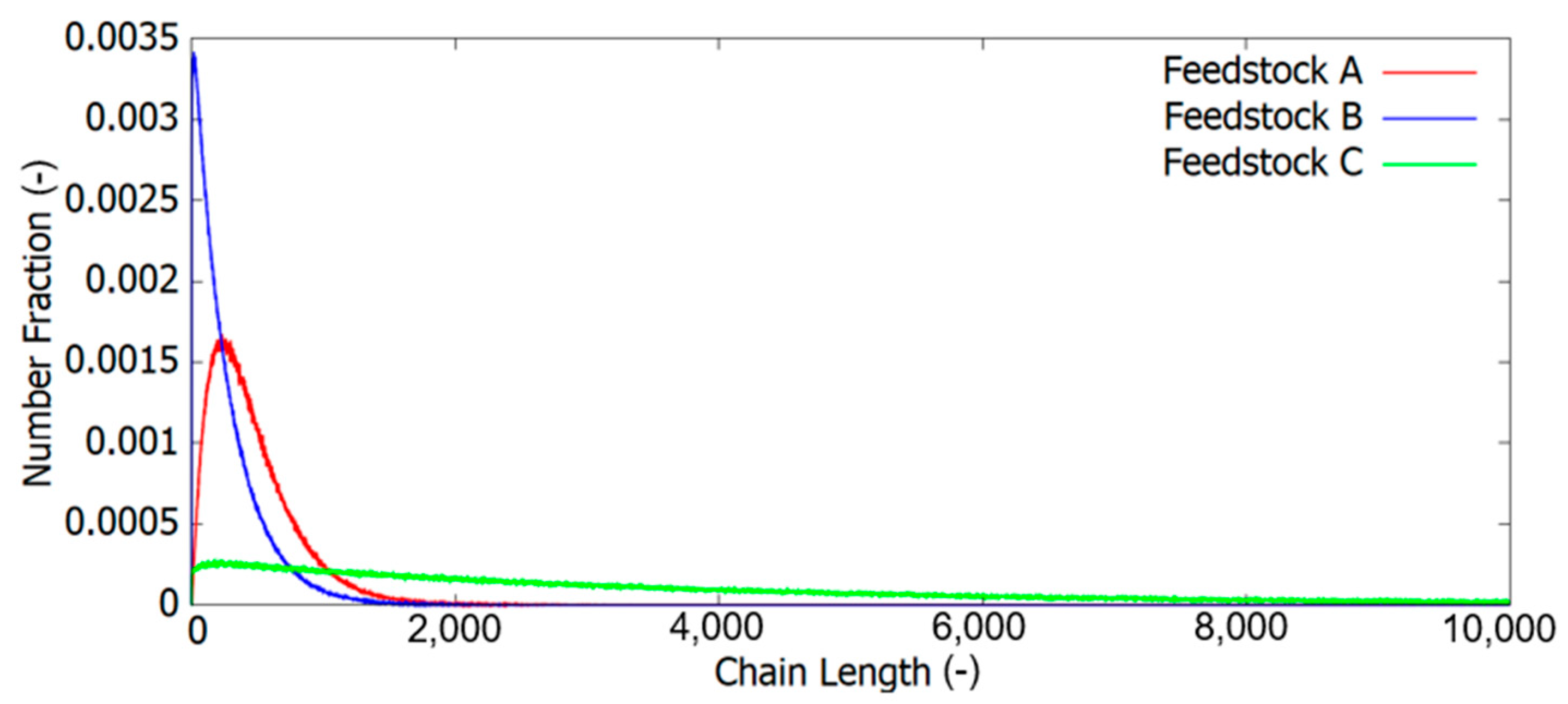
2.2. Generation of Polymer Feedstocks to Study Convergence for Thermochemical Degradation

Out of the ensemble of macromolecules obtained after a converged CMMC synthesis simulation up to 0.2 monomer conversion (i.e., a simulation with an initial monomer amount equal to 5 × 10⁹ for feedstock A and B, and 5 × 10¹⁰ for feedstock C; see Section S1 in the Supporting Information), a number of chains is randomly selected to form the feedstock for the actual thermal degradation simulation. For feedstock A and B, as shown in Table 1, seven cases were specified based on their ${{\displaystyle \sum }}_{i}i·X_{P_i}$, whereas for feedstock C, this was extended to nine as a larger MC control volume was necessary to reach convergence for all degradation characteristics studied. In Table 1, it can be seen that feedstock C contains the same order of magnitude for its number of chains at an ${{\displaystyle \sum }}_{i}i·X_{P_i}$ of 10¹⁰ compared to feedstock A and B, for which ${{\displaystyle \sum }}_{i}i·X_{P_i}$ is 10⁹. The simulation times for the degradation of the three different feedstocks for all cases in Table 1 can be found in Section S2 of the Supporting Information (Table S1 and Figure S1).

For the MC volume calculation during the thermal degradation, only the polymer fraction was taken into account, assuming that the monomer species formed are immediately transferred to the gas phase and degradation reactions only take place in the melt phase. For the plotting of CLDs, a carbon-based conversion (Equation (1)) of 50% is always selected.

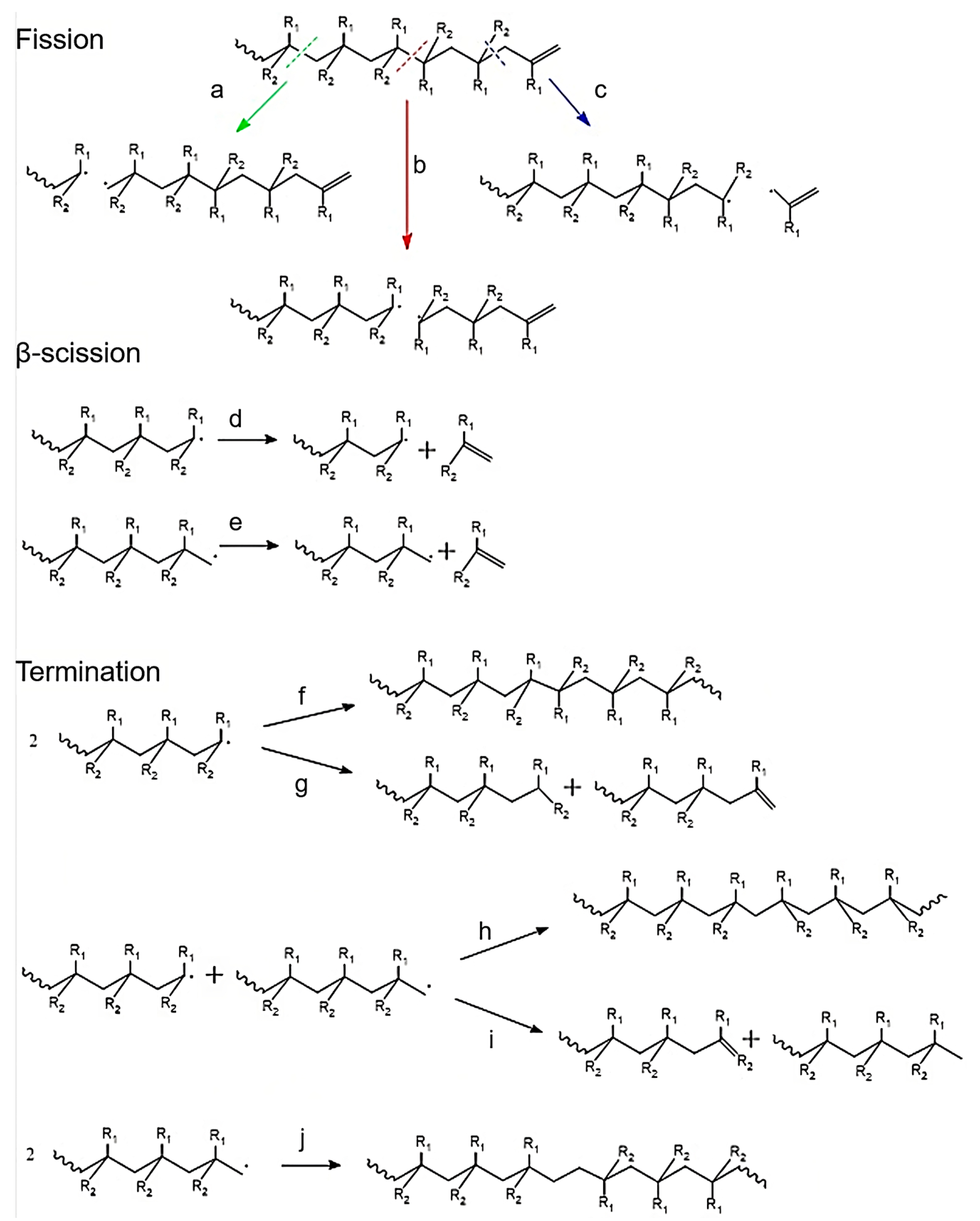
2.3. Degradation Reactions and Kinetic Parameters

Thermochemical degradation is modeled according to the reactions shown in Figure 1, with the average rate coefficients specified in

Table 2. Reactions and (average) kinetic parameters for thermochemical degradation of the vinyl polymer feedstocks A–C in Figure 2; all parameters values are ball-park only in the frame of studying convergence aspects.

Fission Reactions	Reaction a,b	k	Unit
Head–Head Fission	$P_{HH,i}\stackrel{k_{HHF}}{\to }{R}_{x,i-j}+R_{x,j}$	2.0 × 10−2	s−1
Chain End Fission	$P_{=,i}\stackrel{k_{\mathrm{CEF}}}{\to }{R}_{x,i-1}+R_M$	2.0 × 10−4	s−1
Head–Tail Fission	$P_i \stackrel{k_{H\mathrm{T}F}}{\to }{R}_{x,i-j}+R_{p,j}$	2.0 × 10−6	s−1
β-Scissions reactions	Reaction	k	Unit
End chain β-scission (tertiary/secondary radical)	$R_{x,i}^{}\stackrel{k_{ECS,T}}{\to }{R}_{x,i-1}^{}+M$	4.0 × 105	s−1
End chain β-scission (primary radical)	$R_{p,i}^{}\stackrel{k_{\mathrm{ECS},\mathrm{P}}}{\to }{R}_{p,i-1}^{}+M$	2.0 × 105	s−1
Termination reactions	Reaction	k	Unit
Termination between two tertiary/secondary radicals	$R_{x,i}+R_{x,j}\stackrel{k_{\mathrm{t},\mathrm{xx},c}}{\to }{P}_{HH,i+j}$	5.8 × 103	L mol−1 s−1
	$R_{x,i}+R_{x,j}\stackrel{k_{\mathrm{t},\mathrm{xx},d}}{\to }{P}_i+P_{=,j}$	5.8 × 103	L mol−1 s−1
Termination between two primary radicals	$R_{p,i}+R_{p,j}\stackrel{k_{\mathrm{t},PP,c}}{\to }{P}_{TT,i+j}$	1.2 × 104	L mol−1 s−1
Termination between a primary and tertiary/secondary radical	$R_{x,i}^{}+R_{p,j}^{}\stackrel{k_{\mathrm{t},\mathrm{xP},d}}{\to }{P}_{TT,i+j}$	5.8 × 103	L mol−1 s−1
	$R_{x,i}^{}+R_{p,j}^{}\stackrel{k_{\mathrm{t},\mathrm{xP},d}}{\to }{P}_{sat,i}+P_{uns,j}$	5.8 × 103	L mol−1 s−1

^a The first subscript indicates the defect/functionality which needs to be present in the chain to undergo the reaction. ^b Depending on the nature of the vinyl homopolymer, the subscript x stands for a tertiary or secondary end-chain macro radical.

. The term average is used to stress the ignoring of chain length or polymer (mass) fraction dependencies. These average values can be seen as ball-park values for polystyrinics and polyacrylics and are well within the range reported in literature, specifically around 700 K [13,29,43,54]. It should be added that the current work does not aim at a highly accurate description of degradation kinetics of specific vinyl homopolymers, such that ball-park values connected to a basic reaction scheme suffice.

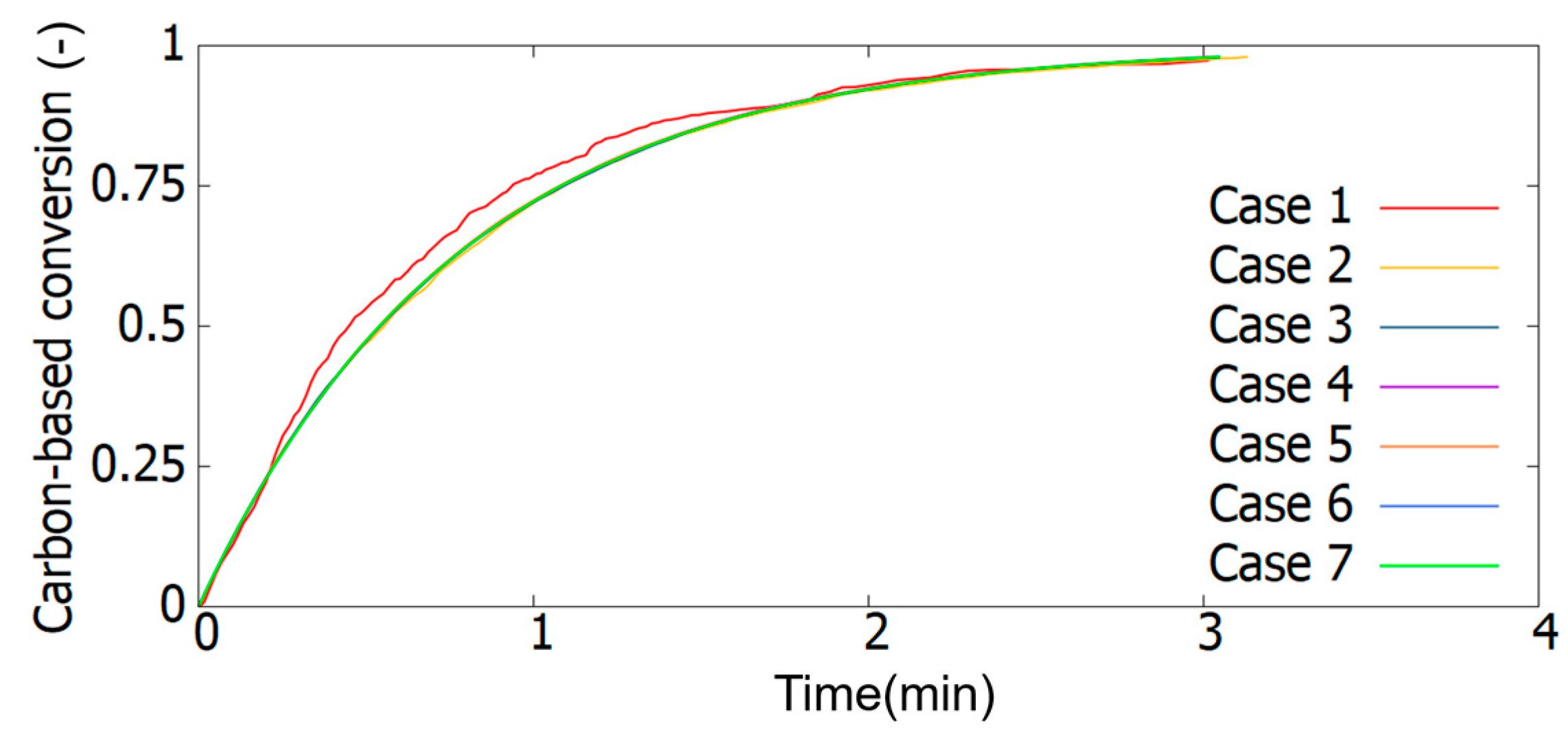
2.4. Thermochemical Degradation Convergence Characteristics

CMMC makes it possible to store and analyze different process characteristics on the level of the individual molecule. In this work, focus is mostly on the main conventional output parameters as common for deterministic solvers, i.e., carbon-based conversion ($con{v}_C$), number average chain length (x_n), mass average chain length ($x_m$), $x_z$, and dispersity (Ð):

$$con{v}_C=\frac{X_{C,product}}{X_{C,0}}$$

(1)

$$x_n=\frac{{{\displaystyle \sum }}_{i}i·X_{P_i}}{{{\displaystyle \sum }}_i{X}_{P_i}}$$

(2)

$$x_m=\frac{{{\displaystyle \sum }}_i{i}^2·X_{P_i}}{{{\displaystyle \sum }}_{i}i·X_{P_i}}$$

(3)

$$x_z=\frac{{{\displaystyle \sum }}_i{i}^3·X_{P_i}}{{{\displaystyle \sum }}_i{i}^2·X_{P_i}}$$

(4)

$$\mathrm{Ð}=\frac{X_m}{X_n}$$

(5)

In these equations, $X_{C,product}$ is the number of carbon atoms present in the (polymer) product at a certain time and $X_{C,0}$ is the number of carbon atoms present in the feedstock at the start of the degradation. In addition to the model outputs listed in Equations (1)–(5), the complete CLD at 0.5 carbon-based conversion and the evolution of the concentration of HH-linkages and UCEs are considered.

All simulations were compiled using the intel (R) Visual Fortran Compiler XE 15.0.6.285 with active compiler optimization on a desktop computer with an Intel i7-8650U processor.

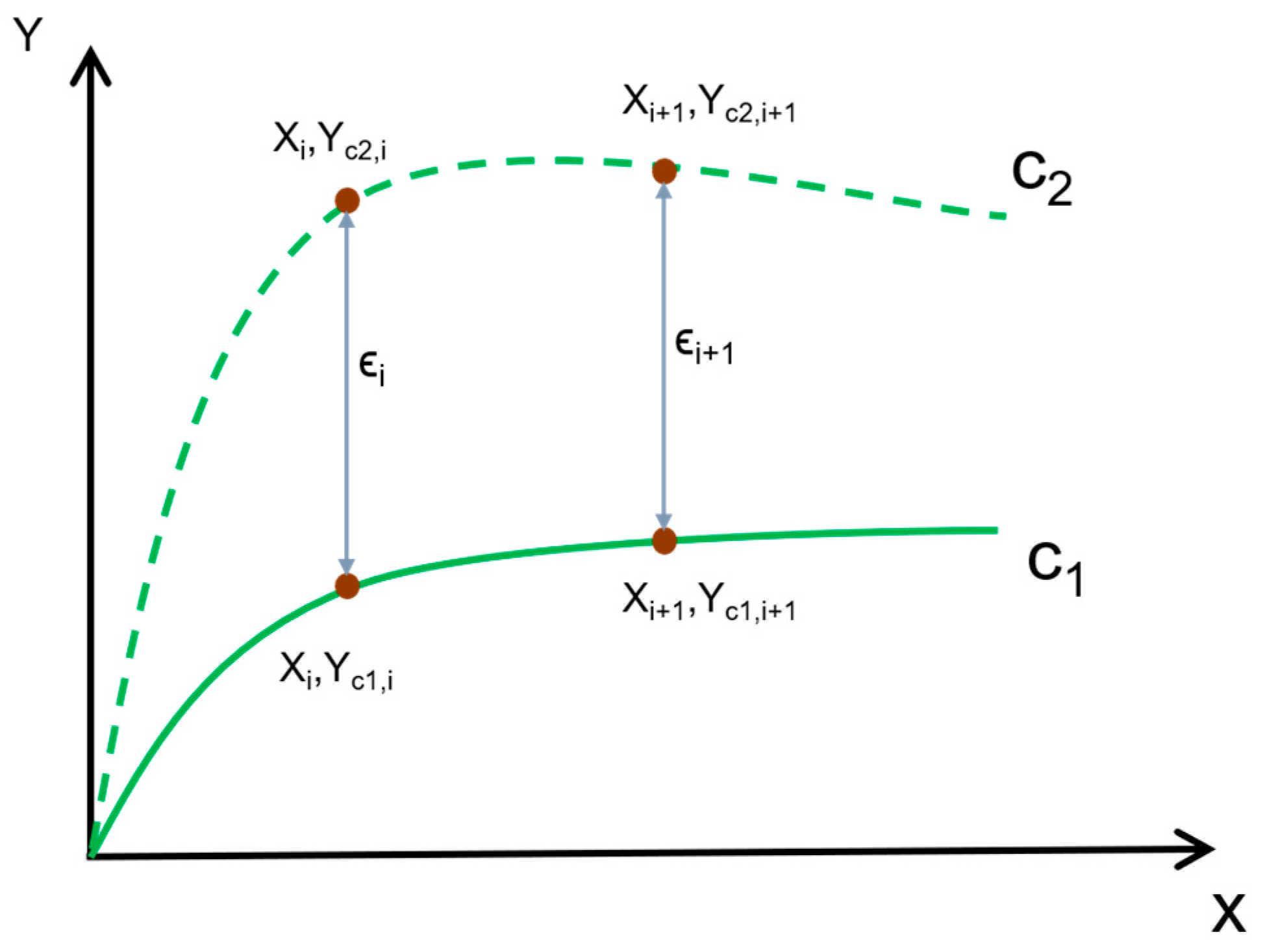
2.5. Convergence Criteria for Thermochemical Degradation

A visual validation regarding convergence was done in a first step by plotting the temporal or carbon-based conversion profiles of the characteristics or model responses of interests with increasing case number, thus increasing MC volume (Table 1).

In a second step, the average relative differences between subsequent cases are mapped according to the principles of Trigilio et al. [19], based on time for the carbon-based conversion and based on a carbon-based conversion range from 0 to 0.95 for the other characteristics. As illustrated in Figure 3, this means that for every model response variable Y, the relative error between two consecutive cases (for simplicity c₁ and c₂) for an observation i for the independent variable X (e.g., a given time or conversion) is initially calculated as:

$${ϵ}_{Y,i,c_1\to c_2}\left(\%\right)=100\times \frac{\left|Y_{c_2,i}-Y_{c_1,i}\right|}{Y_{c_1,i}}$$

(6)

to then obtain an average relative error:

$${ϵ}_{x,c_1\to c_2}\left(\%\right)=\frac{{{\displaystyle \sum }}_i{ϵ}_{Y,i,c_1\to c_2}}{i_{max}}$$

(7)

in which $i_{max}$ is the number of observations for the response.

As in the work of Trigilio et al. [19], a threshold of 1% was used for the convergence determination of conversion, $x_n$, $x_m$, and Ð. For $x_z$, a threshold value of 0.5% was put forward as in previous work on polymerization [19]. Conversion data output was written out every millisecond, and for data plotted as a function of conversion, every 10-3 carbon-based (fractional) conversion.

3. Results and Discussion

In this section, a convergence analysis is presented for the thermochemical degradation of the three feedstocks defined in Figure 2 considering the simulation volumes listed in Table 2. Focus is on the carbon-based conversion ($con{v}_C$), number average chain length ($x_n$), mass average chain length ($x_m$), z-based average chain length ($x_z$), and dispersity (Ð). For each feedstock, both a qualitative visual analysis as well as a quantitative analysis based on the average relative error between two consecutive cases is given, complemented by an inspection of chain length distributions (CLDs) and defect concentration profiles. The converged results are also directly compared considering all feedstocks jointly to highlight the relevance of a sufficiently high number of radicals in the MC control volume.

3.1. Convergence Analysis for Feedstock A with a Low Average Chain Length and Only Head–Head Defects

The model response for which the convergence is checked initially for feedstock A is the carbon-based conversion. As shown in Figure 4, a first visual analysis of the conversion plots for the cases in Table 1 indicates that a satisfactory description is obtained from case 2 onwards. The deviations for the cases with a lower simulation volume from the converged solution (close to case 2) can be explained by the overestimation of structural defects, due to lack of a sufficient number of chains representing the feedstock. As shown in Figure 5, a too high simulated HH-linkages concentration can be seen relative to the converged values.

It should be noted that when the conversion progresses, for every case, the absolute number of defects decreases, together with the volume of the melt phase. Both effects more or less cancel out for converged cases so that a nearly constant concentration of HH-linkages is obtained during thermochemical degradation in Figure 5, bearing in mind that this is the main initiation event for feedstock A. Yet, Figure 5 reveals that mismatches between cases are more evident at higher conversions, specifically for lower case numbers. At a conversion above 0.8, we even see that only for the very high case numbers the stochastic noise is sufficiently low. Inherently, at very high conversions a limited number of chains is left. A way to overcome this is to further increase the initial volume to higher numbers as in Table 1 or to, e.g., duplicate a given composition at a given conversion. However, the added value of such modeling approaches is very limited in view of the extra computational cost.

The differences from the converged numerical results for the simulations with a too low case number become further visible when looking at the average chain length characteristics. In Figure 6, the carbon-based conversion dependencies of $x_n$, $x_m$, $x_z$ and Ð are shown. Case 1 is highly deviating and case 2 is at the edge of acceptable at the lower conversions, whereas the other cases give acceptable results. A deviation from the converged value becomes again most visible above a carbon-based conversion of 0.8, and this now up to case 5. Hence, to properly reflect the (average) chain length characteristics up to high conversions, larger simulation volumes are generally required compared to only a demand of convergence for the conversion.

Besides the visual validation of convergence in Figure 4, Figure 5 and Figure 6, numerical validation of feedstock A was performed according to Equation (7), as shown in

Table 3. Average relative error (%) for the carbon-based conversion $({ϵ}_{con{v}_C})$ the number average chain length (${ϵ}_{x_n}$), mass average chain length (${ϵ}_{x_m}$), dispersity (Ð), and z-average chain length (${ϵ}_{x_z}$) for feedstock A. The starting point of reaching the threshold value (by default 1% but for ${ϵ}_{x_z}$ 0.5%) between two consecutive cases is highlighted in bold italic for each parameter.

Cases	${\mathit{ϵ}}_{\mathit{c}\mathit{o}\mathit{n}{\mathit{v}}_{\mathit{C}}}$ (%)	${\mathit{ϵ}}_{{\mathit{x}}_{\mathit{n}}}$ (%)	${\mathit{ϵ}}_{{\mathit{x}}_{\mathit{m}}}$ (%)	ϵÐ (%)	${\mathit{ϵ}}_{{\mathit{x}}_{\mathit{z}}}$ (%)
1 → 2	4.75	14.65	14.23	2.40	13.58
2 → 3	0.61	1.10	1.33	1.41	2.77
3 → 4	0.35	0.63	0.63	0.28	0.99
4 → 5	0.17	0.27	0.30	0.13	0.61
5 → 6	0.22	0.40	0.45	0.12	0.58
6 → 7	0.09	0.06	0.09	0.08	0.16

for all the model responses covered in Figure 4, Figure 5 and Figure 6. The convergence for conversion is very fast and even for the first case not that far away from the threshold of 1%. For $x_n$, $x_m$ and Ð the convergence is obtained at case 3. For $x_z$, convergence is however only obtained at case 6, highlighting as in the polymerization work of Trigilio et al. [19] and Marien et al. [18] that it is more difficult to calculate the tail of a CLD in an accurate manner.

This can also be seen in Figure 7, in which the (number) CLD for case 1 to 6 is shown with respect to the converged case 7. It is visible that for case 1 and 2, the control volume is so low that the population of chains is so small that one is unable to obtain a proper representation of the CLD. With increasing control volume, a more well-defined CLD becomes visible. Very close to convergence (comparison of case 6 and case 7), it becomes visually nearly impossible to distinguish the two CLDs from each other. From a practical point of view, one could even put forward that the noise in case 5 is already acceptable to obtain a qualitative interpretation. This is supported by the $x_z$ relative error data in Table 3 as the value mentioned for the transition from case 4 to case 5 is only slightly above the threshold of 0.5 (0.61).

3.2. Convergence Analysis for Feedstock B/C with Low/High Average Chain Length and Saturations

In this subsection, a similar discussion to that performed in Figure 4, Figure 5, Figure 6 and Figure 7 and Table 3 for feedstock A is included. It should be remembered that feedstock B is equivalent to feedstock A with the only difference that in addition to termination by recombination (30%), disproportionation (70%) also took place during the prior polymerization. This causes the average chain length of the feedstock to decrease (see Figure 2) and for a fixed control volume results in an increase in the number of chains compared to feedstock A for the degradation simulation (Table 1). Note that feedstock C is obtained via (in silico) polymerization at a lower temperature compared to feedstock B, resulting in lower termination rates with respect to propagation, creating longer chains during synthesis (Figure 2).

In Figure 8, the carbon-based conversion is shown as a function of the time for all seven cases for feedstock B. Compared to feedstock A, feedstock B shows an overall slower thermochemical degradation profile. This is due to the difference in kinetics as there are now also chains present which do not contain HH-bonds. These chains have a slower (degradation) initiation rate and thus an overall slower degradation mechanism. When looking at the conversion plot, one can again see that convergence is visually obtained from case 2 onwards.

The overprediction of the conversion for lower case numbers can again be found in the overprediction in head–head defects, as is shown in Figure 9a. Compared to feedstock A, in feedstock B, both saturated chains and chains with unsaturated chain ends are present. This causes the HH-linkages concentration to decrease more rapidly to a zero value compared to feedstock A. This preferred degradation of chains with HH-linkages causes an increase in the concentration of unsaturated chain ends, as the volume of the remaining polymer chains reduces with this preferred degradation of the chains containing HH-linkages (Figure 9b).

Upon looking at the average chain length characteristics in Figure 10 for feedstock B, the effect of a broader distribution compared to feedstock A becomes visible. As the population consists of more chains, for a given MC control volume, the number average chain length $x_n$ is already well-defined from case 2 onwards. For $x_m$ and $x_z$, more stochastic noise results for case 2 and 3 compared to $x_n$ as it remains challenging to represent the tail more accurately, bearing in mind the initial shape difference in both feedstock CLDs. This convergence delaying effect also become visible in the dispersity plot where we see convergence from case 4 onwards. Furthermore, as for feedstock A, the increase in noise at the end of the simulation becomes more visible with an inherent reduction in the number of chains as a function of conversion.

In Figure 10, we can also see a significant drop of the (average) chain lengths of the polymer compared to feedstock A (Figure 6). For feedstock A, all chains are mainly initiated by HH-fission, with no direct chain length-dependent probability of which chains initiate primarily. This results in a gradual reduction of the number of chains over the polymer population and thus only slightly changing average properties. For feedstock B, in contrast, chains with HH-bonds are mainly longer chains in the population thus when these first start to degrade the average chain length drops. Moreover, longer chains contain more HT-linkages, making longer chains statistically more susceptible to HT-fission than shorter chains, thus resulting in an additional lowering of the average chain lengths during degradation.

Again, we included results based on the average relative error (Equation (7)) as well. As shown in

Table 4. Average relative error (%) for the carbon-based conversion $({ϵ}_{con{v}_C})$ the number average chain length (${ϵ}_{x_n}$), mass average chain length (${ϵ}_{x_m}$), dispersity (Ð), and z-average chain length (${ϵ}_{x_z}$) for feedstock B. The starting point of reaching the threshold value (by default 1% but for ${ϵ}_{x_z}$ 0.5%) between two consecutive cases is highlighted in bold italic for each parameter.

Cases	ϵconversion (%)	${\mathit{ϵ}}_{{\mathit{x}}_{\mathit{n}}}$ (%)	${\mathit{ϵ}}_{{\mathit{x}}_{\mathit{m}}}$ (%)	ϵÐ (%)	${\mathit{ϵ}}_{{\mathit{x}}_{\mathit{z}}}$ (%)
1 → 2	21.03	3.23	5.16	6.86	11.91
2 → 3	0.25	0.67	1.51	1.22	3.22
3 → 4	0.13	0.68	0.64	0.56	1.05
4 → 5	0.09	0.38	0.78	0.41	1.42
5 → 6	0.03	0.20	0.23	0.13	0.31
6 → 7	0.02	0.06	0.07	0.03	0.13

, one can see that already from case 2 onwards convergence is obtained in terms of the carbon-based conversion. Similarly, $x_n$ convergence is secured from case 2 onwards, yet $x_m$ and consequently Ð converge only later, more specifically from case 3 onwards. The average relative error on $x_z$ goes below 0.5 % only from case 5 onwards, again highlighting the more difficult convergence of the tail, confirming the necessary minimal representation of the heavier fraction of chains of the polymer distribution.

The obtaining of convergence only from case 5 onwards for x_z is also visually observable when looking at the number CLD of the different cases in Figure 11. The heavily underrepresented population is clearly visible for case 1 and 2, as it struggles to even represent the form of the distribution itself. For case 3 and 4, noise is still noticeable yet the general form of the CLD becomes more pronounced. Almost noise-free simulations result for case 5 and 6, consistent with highly converged result for case 7.

For feedstock C, similar figures to those for Figure 8, Figure 9, Figure 10 and Figure 11 are included in Supporting Information (Section S3; Figures S3–S6). It follows that compared to the previous feedstocks, convergence is reached only for larger MC control volumes, which can be expected as for a given MC volume less chains are present knowing that for feedstock C most of the starting chains are quite long. For example, the carbon-based convergence in Figure S3 is only reasonable from case 3 onwards (before case 2). However, we can still see some stochastic noise in case 3 so that one could say that a dedicated convergence requires even a higher case number. When looking at the variation of the concentration of HH-linkages in Figure S4, the limitations of the very low number of chains (only 30) representing the polymer feedstock in case 1 are very evident. Moreover, even for cases 2, 3, and 4, very clear visual differences in HH-linkage concentrations are noticeable, this in contrast to the results before. Pronounced deviations are also observed in case 1 and 2 for the concentration of unsaturated chain ends (Figure S5b).

This slower convergence for cases 1, 2, and 3 compared to the other feedstocks is also evident for the average chain length characteristics in Figure S5. By looking at $x_n$ in Figure S5, the effect of the limited number of chains is clearly visible for case 1. We can say that visually, convergence is only obtained from case 4 onwards. For $x_m$ and $x_z$, a stronger deviation of the converged values is visible due to the higher kinetic influence of the longer chains, as shown by the fast drops in Figure S5b,c. Due to the presence of many larger chains, this part of the chain population decreases faster compared to feedstock A and B, leading to a faster underrepresentation of the feedstock’s chain population with decreasing simulation volume, resulting in turn in an increase in stochastic noise with increasing carbon-based conversion. For $x_m$ and Ð, convergence is therefore only obtained from case 5 onwards and for $x_z$, convergence is only obtained from case 6 onwards.

The average relative errors in Table S4 of the Supporting Information for thermochemical degradation of feedstock C show that convergence is only reached from case 4 onwards for most model responses considered. It should however be noted that for the carbon-based conversion, convergence is obtained if the order of magnitude of number of chains present in the simulation volume is the same as for case 2 regarding feedstock A and B (10³). This trend is also visible for Ð, $x_m$, and $x_z$, highlighting the relevance of the number of chains in a general degradation simulation Furthermore, for Ð and $x_n$, the convergence criteria of an average relative error below 1% are met from case 5 onwards and for $x_m$ from case 4 onwards. For $x_z$, convergence is obtained from case 7 onwards. This more demanding simulation volume for $x_z$ is consistent with the (number) CLD data in Figure S6, showing that only for very high case numbers (8 or 9) can a quantitative CLD description be claimed. Practically, however, one could already select case 7.

3.3. Number of Radicals for Thermochemical Simulations for Feedstocks A, B, and C

A summary of the (sufficiently) converged simulation results as obtained considering case 7 for conversion (a), $x_n$ (b), $x_m$ (c), and $x_z$ (d) for feedstocks A, B, and C is provided in Figure 12. Feedstock A degrades the fastest as it contains only short chains with HH-linkages. Feedstock B degrades the slowest as it contains the most saturated chains without HH defects, which thus have to initiate via slower random HT-fission. Compared to feedstock A, which maintains a nearly constant average chain length of 460 during degradation, feedstock B and C show a steady reduction in average chain length with increasing conversion. This can be explained by the mixed termination modes during the prior synthesis of feedstock B and C, which results in longer chains containing HH-defects that preferentially undergo fission compared to shorter chains lacking a HH-defect. These chain length dependencies indicate that, in a more detailed modeling approach, it could be worthwhile to account for chain length dependencies on the rate coefficient level as opposed to the averages values as used in this present work (Table 2).

Figure 13 displays the corresponding variation for the number of radicals in the MC control volume. For all three feedstocks, a similar trend is observed at first sight. The number of radicals is the highest at the start of the degradation and diminishes with increasing conversion, as the number of chains and defects, and thus potential radical sources diminishes. A closer inspection of Figure 13 reveals that the feedstock has an impact on the absolute radical numbers. As explained above, the difference between feedstock A and B is mainly due to the difference in concentration of HH-linkages (Figure 5 vs. Figure 9a). Consistently, we see in Figure 13 that for feedstock B, the number of radicals follows the trend of the concentration of HH-linkages with once no more HH-linkages present, only new radicals formed at a slower rate from HT- and UCE-fission (blue data points closer to the x-axis). Furthermore, for feedstock C, as the chains are significantly longer, the average time to fully unzip a macroradical formed via HH-fission is longer compared to feedstock A and B, resulting in a higher average number of radicals at the start of the degradation.

In

Table 5. Maximum number of radicals in control volume for Figure 12 (case 7) and other cases in Table 1.

Case	${{\displaystyle \sum }}_{\mathit{i}}\mathit{i}·{\mathit{X}}_{{\mathit{P}}_{\mathit{i}}}$	Maximum Number of Radicals at a Certain Time
		A	B	C
1	1.0 × 105	2	2	2
2	1.0 × 106	4	4	4
3	1.0 × 107	8	6	8
4	5.0 × 107	15	11	13
5	1.0 × 108	24	13	20
6	5.0 × 108	61	29	59
7	1.0 × 109	106	44	106
8	5.0 × 109	-	-	401
9	1.0 × 1010	-	-	776

, for all three feedstocks, the maximum number of radicals coexisting at a certain time is shown for all cases. It can be seen that for case 1, for all three feedstocks, the maximum number of radicals during the thermal degradation is only two, which is the bare minimum as a fission results in the formation of two radicals at the same time. It is interesting to see that, for the considered thermochemical degradation conditions, even once sufficient convergence is established, the maximum number of radicals is rather limited compared to previously studied (intrinsic) polymerization conditions, even if larger synthesis simulation volumes are considered [19,55,56]. Furthermore, for feedstock A and C, one can almost see a linear trend for the number of radicals coexisting simultaneously with increasing control volume once converged for the higher case numbers.

Note that the variation of the number of radicals is from a kinetic point of view less easy to grasp. To allow for a better kinetic comparison, it is more interesting to work with radical concentration variations, as done in Figure 14. It follows that a too low simulation volume causes a significant fluctuation of the radical concentration with respect to the converged value. For feedstock A and B, this convergence is obtained for case 7 and for feedstock C for case 9, highlighting that a convergence of radical concentrations is on the level of the tail of a number CLD. Fluctuating radical concentrations can however be enough to obtain convergence for average model responses, as highlighted above. However, too low case numbers give too high fluctuations. For example, in case 1 of feedstock A, an extreme fluctuation from 0 to 5 × 10⁻⁴ mol·L⁻¹ compared to the converged case with a value fluctuating around 5 × 10⁻⁷ mol·L⁻¹ can be observed (Figure S7). This deviation of case 1 compared to the converged case becomes even more significant towards the end of the conversion with even radical concentrations reaching 2 × 10⁻³ mol·L⁻¹, far above the converged value.

A similar trend is visible for the other two feedstocks in Figure 14 both showing a narrowing down of the radical concentration fluctuation with increasing simulation volume. For feedstock C, the delayed convergence is again evident. For example, for both cases 1 and 2, the limited number of chains present is causing strong fluctuations and one needs higher case numbers (case 8 or 9) to rule out a significant fluctuation effect.

4. Conclusions

To obtain a low simulation time without compromising the accuracy of the model predictions, a key aspect of a kMC simulation is the selection of the lowest MC control volume that leads to converged results. In this work, for the thermochemical degradation of vinyl polymers such as polyacrylics and polystyrinics with dominant unzipping, the convergence demands of three feedstocks, covering various chain length ranges and amounts of structural defects, has therefore been investigated based on visual inspection and by calculating relative errors based on polymerization-based literature threshold values for the carbon-based conversion, number, mass, z-based average chain length, and dispersity. The number of chains has shown to be a key parameter to obtain sufficient convergence. A certain degree of noise can be admitted at very high carbon-based conversions, as inherently a reduction in the number of chains is taking place.

Based on the kinetic rates obtained in this work, it is shown that the start of the thermal degradation of vinyl polymers is mainly defined by HH-fission. A competition between UCE- and HT-fission then follows which is more chain length-dependent. It has been further demonstrated that reaching convergence for chain length averages is the most demanding, especially for a feedstock having a broad CLD with a very long tail. In addition, a link with the concentration of head–head defects and unsaturated chain ends, as well as with the complete chain length distribution has been made. The (maximum) number of radicals has been identified as well, with lower numbers detected as under polymerization conditions.

The current work thus further contributes to the bridging of the polymer reaction engineering field in both synthesis and recycling. Future work will be directed to more complex polymer systems and more detailed modeling approaches, including appropriate model reduction tools.

References

1. Ghasem, N. Computer Methods in Chemical Engineering; CRC Press: Boca Raton, FL, USA, 2021. [Google Scholar]
2. Mostoufi, N.; Constantinides, A. Applied Numerical Methods for Chemical Engineers; Academic Press: Cambridge, MA, USA, 2022. [Google Scholar]
3. Trigilio, A.D.; Marien, Y.W.; Van Steenberge, P.H.; D’hooge, D.R. Gillespie-driven kinetic Monte Carlo algorithms to model events for bulk or solution (bio) chemical systems containing elemental and distributed species. Ind. Eng. Chem. Res. 2020, 59, 18357–18386. [Google Scholar] [CrossRef]
4. Wiehe, I.A. A phase-separation kinetic model for coke formation. Ind. Eng. Chem. Res. 1993, 32, 2447–2454. [Google Scholar] [CrossRef]
5. Sabbe, M.K.; Reyniers, M.-F.; Reuter, K. First-principles kinetic modeling in heterogeneous catalysis: An industrial perspective on best-practice, gaps and needs. Catal. Sci. Technol. 2012, 2, 2010–2024. [Google Scholar] [CrossRef]
6. Mei, D.; Neurock, M.; Smith, C.M. Hydrogenation of acetylene–ethylene mixtures over Pd and Pd–Ag alloys: First-principles-based kinetic Monte Carlo simulations. J. Catal. 2009, 268, 181–195. [Google Scholar] [CrossRef]
7. Broadbelt, L.J.; Stark, S.M.; Klein, M.T. Computer generated pyrolysis modeling: On-the-fly generation of species, reactions, and rates. Ind. Eng. Chem. Res. 1994, 33, 790–799. [Google Scholar] [CrossRef]
8. Liu, R.; Armaou, A.; Chen, X. Adaptable parallel acceleration strategy for dynamic Monte Carlo simulations of polymerization with microscopic resolution. Ind. Eng. Chem. Res. 2021, 60, 6173–6187. [Google Scholar] [CrossRef]
9. Edeleva, M.; Marien, Y.W.; Van Steenberge, P.H.; D’hooge, D.R. Jacket temperature regulation allowing well-defined non-adiabatic lab-scale solution free radical polymerization of acrylates. React. Chem. Eng. 2021, 6, 1053–1069. [Google Scholar] [CrossRef]
10. Van Steenberge, P.H.M.; D’hooge, D.R.; Wang, Y.; Zhong, M.; Reyniers, M.-F.; Konkolewicz, D.; Matyjaszewski, K.; Marin, G.B. Linear Gradient Quality of ATRP Copolymers. Macromolecules 2012, 45, 8519–8531. [Google Scholar] [CrossRef]
11. Figueira, F.L.; Wu, Y.-Y.; Zhou, Y.-N.; Luo, Z.-H.; Van Steenberge, P.H.; D’hooge, D.R. Coupled matrix kinetic Monte Carlo simulations applied for advanced understanding of polymer grafting kinetics. React. Chem. Eng. 2021, 6, 640–661. [Google Scholar] [CrossRef]
12. De Keer, L.; Kilic, K.I.; Van Steenberge, P.H.; Daelemans, L.; Kodura, D.; Frisch, H.; De Clerck, K.; Reyniers, M.-F.; Barner-Kowollik, C.; Dauskardt, R.H. Computational prediction of the molecular configuration of three-dimensional network polymers. Nat. Mater. 2021, 20, 1422–1430. [Google Scholar] [CrossRef]
13. De Smit, K.; Marien, Y.W.; Van Geem, K.M.; Van Steenberge, P.H.M.; D’Hooge, D.R. Connecting polymer synthesis and chemical recycling on a chain-by-chain basis: A unified matrix-based kinetic Monte Carlo strategy. React. Chem. Eng. 2020, 5, 1909–1928. [Google Scholar] [CrossRef]
14. De Smit, K.; Marien, Y.; Van Steenberge, P.; D’hooge, D.R.; Edeleva, M. Playing with process conditions to increase the industrial sustainability of poly (lactic acid)-based materials. React. Chem. Eng. 2023. [Google Scholar] [CrossRef]
15. Wu, Y.-Y.; Figueira, F.L.; Van Steenberge, P.H.; D’hooge, D.R.; Zhou, Y.-N.; Luo, Z.-H. Bridging principal component analysis and method of moments based parameter estimation for grafting of polybutadiene with styrene. Chem. Eng. J. 2021, 425, 130463. [Google Scholar] [CrossRef]
16. Mastan, E.; Zhu, S. Method of moments: A versatile tool for deterministic modeling of polymerization kinetics. Eur. Polym. J. 2015, 68, 139–160. [Google Scholar] [CrossRef]
17. De Keer, L.; Figueira, F.L.; Marien, Y.W.; De Smit, K.; Edeleva, M.; Van Steenberge, P.H.; D’hooge, D.R. Benchmarking stochastic and deterministic kinetic modeling of bulk and solution radical polymerization processes by including six types of factors two. Macromol. Theory Simul. 2020, 29, 2000065. [Google Scholar] [CrossRef]
18. Marien, Y.W.; Edeleva, M.; Figueira, F.L.; Arraez, F.J.; Van Steenberge, P.H.; D’hooge, D.R. Translating simulated chain length and molar mass distributions in chain-growth polymerization for experimental comparison and mechanistic insight. Macromol. Theory Simul. 2021, 30, 2100008. [Google Scholar] [CrossRef]
19. Trigilio, A.D.; Marien, Y.W.; Van Steenberge, P.H.; D’hooge, D.R. Toward an Automated Convergence Tool for Kinetic Monte Carlo Simulation of Conversion, Distributions, and Their Averages in Non-dispersed Phase Linear Chain-Growth Polymerization. Ind. Eng. Chem. Res. 2023, 62, 2583–2593. [Google Scholar] [CrossRef]
20. Rego, A.S.; Amaral, A.M.; Brandão, A.L. Monte Carlo simulation of terpolymerization: Optimizing the simulation and post-processing times. Can. J. Chem. Eng. 2023. [Google Scholar] [CrossRef]
21. Gao, H.; Oakley, L.H.; Konstantinov, I.A.; Arturo, S.G.; Broadbelt, L.J. Acceleration of Kinetic Monte Carlo Method for the Simulation of Free Radical Copolymerization through Scaling. Ind. Eng. Chem. Res. 2015, 54, 11975–11985. [Google Scholar] [CrossRef]
22. Nasresfahani, A.; Hutchinson, R.A. Modeling the Distribution of Functional Groups in Semibatch Radical Copolymerization: An Accelerated Stochastic Approach. Ind. Eng. Chem. Res. 2018, 57, 9407–9419. [Google Scholar] [CrossRef]
23. Trigilio, A.D.; Marien, Y.W.; Edeleva, M.; Van Steenberge, P.H.; D’hooge, D.R. Optimal search methods for selecting distributed species in Gillespie-based kinetic Monte Carlo. Comput. Chem. Eng. 2022, 158, 107580. [Google Scholar] [CrossRef]
24. Nanda, S.; Berruti, F. Thermochemical conversion of plastic waste to fuels: A review. Environ. Chem. Lett. 2021, 19, 123–148. [Google Scholar] [CrossRef]
25. Rahimi, A.; García, J.M. Chemical recycling of waste plastics for new materials production. Nat. Rev. Chem. 2017, 1, 0046. [Google Scholar] [CrossRef]
26. Yao, Z.; Reinmöller, M.; Ortuño, N.; Zhou, H.; Jin, M.; Liu, J.; Luque, R. Thermochemical conversion of waste printed circuit boards: Thermal behavior, reaction kinetics, pollutant evolution and corresponding controlling strategies. Prog. Energy Combust. Sci. 2023, 97, 101086. [Google Scholar] [CrossRef]
27. Moens, E.K.; De Smit, K.; Marien, Y.W.; Trigilio, A.D.; Van Steenberge, P.H.; Van Geem, K.M.; Dubois, J.-L.; D’hooge, D.R. Progress in reaction mechanisms and reactor technologies for thermochemical recycling of poly (methyl methacrylate). Polymers 2020, 12, 1667. [Google Scholar] [CrossRef] [PubMed]
28. Coile, M.W.; Harmon, R.E.; Wang, G.; SriBala, G.; Broadbelt, L.J. Kinetic Monte Carlo Tool for Kinetic Modeling of Linear Step-Growth Polymerization: Insight into Recycling of Polyurethanes. Macromol. Theory Simul. 2022, 31, 2100058. [Google Scholar] [CrossRef]
29. Dogu, O.; Pelucchi, M.; Van de Vijver, R.; Van Steenberge, P.H.; D’hooge, D.R.; Cuoci, A.; Mehl, M.; Frassoldati, A.; Faravelli, T.; Van Geem, K.M. The chemistry of chemical recycling of solid plastic waste via pyrolysis and gasification: State-of-the-art, challenges, and future directions. Prog. Energy Combust. Sci. 2021, 84, 100901. [Google Scholar] [CrossRef]
30. Shi, C.; Reilly, L.T.; Kumar, V.S.P.; Coile, M.W.; Nicholson, S.R.; Broadbelt, L.J.; Beckham, G.T.; Chen, E.Y.-X. Design principles for intrinsically circular polymers with tunable properties. Chem 2021, 7, 2896–2912. [Google Scholar] [CrossRef]
31. Pires da Mata Costa, L.; Brandão, A.L.T.; Pinto, J.C. Modeling of polystyrene degradation using kinetic Monte Carlo. J. Anal. Appl. Pyrolysis 2022, 167, 105683. [Google Scholar] [CrossRef]
32. Kruse, T.M.; Woo, O.S.; Broadbelt, L.J. Detailed mechanistic modeling of polymer degradation: Application to polystyrene. Chem. Eng. Sci. 2001, 56, 971–979. [Google Scholar] [CrossRef]
33. Kruse, T.M.; Wong, H.-W.; Broadbelt, L.J. Mechanistic modeling of polymer pyrolysis: Polypropylene. Macromolecules 2003, 36, 9594–9607. [Google Scholar] [CrossRef]
34. Pereira, G.; Venturini, A.; Silvestri, T.; Dapieve, K.; Montagner, A.; Soares, F.; Valandro, L. Low-temperature degradation of Y-TZP ceramics: A systematic review and meta-analysis. J. Mech. Behav. Biomed. Mater. 2016, 55, 151–163. [Google Scholar] [CrossRef] [PubMed]
35. McKenna, T.F.; Soares, J.B. Single particle modelling for olefin polymerization on supported catalysts: A review and proposals for future developments. Chem. Eng. Sci. 2001, 56, 3931–3949. [Google Scholar] [CrossRef]
36. Asua, J.M. Emulsion polymerization: From fundamental mechanisms to process developments. J. Polym. Sci. Part A Polym. Chem. 2004, 42, 1025–1041. [Google Scholar] [CrossRef]
37. Busch, M. Modeling Kinetics and Structural Properties in High-Pressure Fluid-Phase Polymerization. Macromol. Theory Simul. 2001, 10, 408–429. [Google Scholar] [CrossRef]
38. Zhou, Y.-N.; Li, J.-J.; Wu, Y.-Y.; Luo, Z.-H. Role of external field in polymerization: Mechanism and kinetics. Chem. Rev. 2020, 120, 2950–3048. [Google Scholar] [CrossRef]
39. Martinez, M.R.; Schild, D.; De Luca Bossa, F.; Matyjaszewski, K. Depolymerization of Polymethacrylates by Iron ATRP. Macromolecules 2022, 55, 10590–10599. [Google Scholar] [CrossRef]
40. Dogu, O.; Plehiers, P.P.; Van de Vijver, R.; D’hooge, D.R.; Van Steenberge, P.H.; Van Geem, K.M. Distribution changes during thermal degradation of poly (styrene peroxide) by pairing tree-based kinetic Monte Carlo and artificial intelligence tools. Ind. Eng. Chem. Res. 2021, 60, 3334–3353. [Google Scholar] [CrossRef]
41. Ordaz-Quintero, A.; Monroy-Alonso, A.; Saldívar-Guerra, E. Thermal Pyrolysis of Polystyrene Aided by a Nitroxide End-Functionality. Experiments and Modeling. Processes 2020, 8, 432. [Google Scholar] [CrossRef]
42. Siddiqui, M.N.; Redhwi, H.H.; Achilias, D.S. Simulation of the thermal degradation kinetics of biobased/biodegradable and non-biodegradable polymers using the random chain-scission model. Capabilities and limitations. J. Anal. Appl. Pyrolysis 2022, 168, 105767. [Google Scholar] [CrossRef]
43. Eli, K.C.; Moens, Y.W.M. Chapter 6: Design of Lab-Scale Depolymerization Experiments; De Gruyter: Berlin, Germany, 2023. [Google Scholar]
44. Aboulkas, A.; El Bouadili, A. Thermal degradation behaviors of polyethylene and polypropylene. Part I: Pyrolysis kinetics and mechanisms. Energy Convers. Manag. 2010, 51, 1363–1369. [Google Scholar] [CrossRef]
45. Manring, L.E. Thermal degradation of poly (methyl methacrylate). 2. Vinyl-terminated polymer. Macromolecules 1989, 22, 2673–2677. [Google Scholar] [CrossRef]
46. Kashiwagi, T.; Hirata, T.; Brown, J.E. Thermal and oxidative degradation of poly (methyl methacrylate) molecular weight. Macromolecules 1985, 18, 131–138. [Google Scholar] [CrossRef]
47. Hirata, T.; Kashiwagi, T.; Brown, J.E. Thermal and oxidative degradation of poly (methyl methacrylate): Weight loss. Macromolecules 1985, 18, 1410–1418. [Google Scholar] [CrossRef]
48. Manring, L.E.; Sogah, D.Y.; Cohen, G.M. Thermal degradation of poly (methyl methacrylate). 3. Polymer with head-to-head linkages. Macromolecules 1989, 22, 4652–4654. [Google Scholar] [CrossRef]
49. Manring, L.E. Thermal degradation of saturated poly (methyl methacrylate). Macromolecules 1988, 21, 528–530. [Google Scholar] [CrossRef]
50. Faravelli, T.; Pinciroli, M.; Pisano, F.; Bozzano, G.; Dente, M.; Ranzi, E. Thermal degradation of polystyrene. J. Anal. Appl. Pyrolysis 2001, 60, 103–121. [Google Scholar] [CrossRef]
51. Nakamura, Y.; Yamago, S. Termination mechanism in the radical polymerization of methyl methacrylate and styrene determined by the reaction of structurally well-defined polymer end radicals. Macromolecules 2015, 48, 6450–6456. [Google Scholar] [CrossRef]
52. De Keer, L.; Van Steenberge, P.H.; Reyniers, M.F.; Marin, G.B.; Hungenberg, K.D.; Seda, L.; D’hooge, D.R. A complete understanding of the reaction kinetics for the industrial production process of expandable polystyrene. AIChE J. 2017, 63, 2043–2059. [Google Scholar] [CrossRef]
53. Tefera, N.; Weickert, G.; Westerterp, K. Modeling of free radical polymerization up to high conversion. II. Development of a mathematical model. J. Appl. Polym. Sci. 1997, 63, 1663–1680. [Google Scholar] [CrossRef]
54. Ferriol, M.; Gentilhomme, A.; Cochez, M.; Oget, N.; Mieloszynski, J. Thermal degradation of poly (methyl methacrylate)(PMMA): Modelling of DTG and TG curves. Polym. Degrad. Stab. 2003, 79, 271–281. [Google Scholar] [CrossRef]
55. Tripathi, A.; Sundberg, D. A Hybrid Algorithm for Accurate and Efficient Monte Carlo Simulations of Free-Radical Polymerization Reactions. Macromol. Theory Simul. 2014, 24, 52–64. [Google Scholar] [CrossRef]
56. Ali Parsa, M.; Kozhan, I.; Wulkow, M.; Hutchinson, R.A. Modeling of functional group distribution in copolymerization: A comparison of deterministic and stochastic approaches. Macromol. Theory Simul. 2014, 23, 207–217. [Google Scholar] [CrossRef]
Figure 1. Basic reaction scheme for thermochemical degradation of a general vinyl polymer; to not overload the figure, a theoretical starting chain containing all defects/functionalities is shown. Initiation occurs via head–tail fission (a), head–head fission (b), and end-chain fission with the formed small radical assumed to go the gas phase similar as the monomer (c). Depropagation occurs via end-chain β-scission of the formed secondary/tertiary (d) and primary (e) end-chain macroradical. Termination can take place between two secondary/tertiary macroradicals via recombination (f) or disproportionation (g), or between a primary and a secondary/tertiary macroradical via combination (h) or disproportionation (i), or between two primary radicals via recombination forming a tail–tail linkage (j). The radical type (secondary vs. tertiary) depends on R1 and R2 being a hydrogen or not.
Processes 11 01623 g001
Figure 2. Number chain length distribution for feedstock A, B, and C to start a thermochemical degradation. Polymerization simulation conditions to obtain these feedstocks can be found in the Supporting Information (S1).
Processes 11 01623 g002
Figure 3. Conceptual representation of the relative difference in error (ϵx,i,c_1→c_2) between two discreet observations for two generic cases (c1 and c2) for the model response Y [19].
Processes 11 01623 g003
Figure 4. Effect of the MC control volume (Table 2) on the simulated carbon-based conversion profile for thermochemical degradation of feedstock A (Figure 1); kinetic parameters in Table 2.
Processes 11 01623 g004
Figure 5. Effect of the MC control volume on Head-Head linkages during thermochemical degradation expressed in mol·L−1 for feedstock A.
Processes 11 01623 g005
Figure 6. Effect of the MC control volume on the evolution of (a) the number average chain length ( x n ), (b) mass average chain length ( x m ), (c) z-average chain length ( x z ), and (d) dispersity (Ð) during thermochemical degradation of feedstock A (Figure 1); model parameters: Table 2.
Processes 11 01623 g006
Figure 7. Number chain length distribution (CLD) at a carbon-based conversion of 0.5 for feedstock A for several cases with the highly converged CLD corresponding to Case 7 included in all subplots for comparison; (a) case 1, (b) case 2, (c) case 3 and 4, (d) case 5 and 6. Pragmatically, case 5 is already very close to the converged one.
Processes 11 01623 g007
Figure 8. Effect of the MC control volume (Table 2) on the simulated carbon-based conversion profile for thermochemical degradation of feedstock B (Figure 1); kinetic parameters in Table 1.
Processes 11 01623 g008
Figure 9. Effect of the MC control volume on the concentration of (a) head–head linkages during thermochemical degradation of feedstock B and (b) the concentration of head–tail linkages expressed in mol·L−1.
Processes 11 01623 g009
Figure 10. Effect of simulation volume on the evolution of the (a) number average chain length ( x n ), (b) mass average chain length ( x m ), (c) z-average chain length ( x z ), and (d) dispersity (Ð), during thermal degradation of Feedstock C; model parameters: Table 1, SI.
Processes 11 01623 g010
Figure 11. Number chain length distribution (CLD) at a carbon-based conversion of 50% for feedstock B for several cases with the CLD corresponding to case 7 included in all subplots for comparison; (a) case 1, (b) case 2, (c) case 3 and 4, (d) case 5 and 6.
Processes 11 01623 g011
Figure 12. Comparison of sufficiently converged results (case 7 in Table 1); Carbon-based conversion (a), number average chain length ( x n ) (b), mass average chain length ( x m ) (c) and z-average chain length ( x z ), (d) for feedstock A (red), feedstock B (blue), and feedstock C (green); kinetic parameters: Table 2.
Processes 11 01623 g012
Figure 13. Corresponding radical number variations for Figure 12. Plot with line provided in the Supporting Information (Figure S7).
Processes 11 01623 g013
Figure 14. Radical concentration during the thermal degradation of feedstock A (cases 1 to 4 on the top left and 4 to 7 on the top right), feedstock B (cases 1 to 4 on the center left and 4 to 7 on the center right), and feedstock C (cases 1 to 5 on the bottom left and 5 to 9 on the bottom right). Line plots can be found in the Supporting information (Figure S7).
Processes 11 01623 g014