Continuous Reactor Temperature Control with Optimized PID Parameters Based on Improved Sparrow Algorithm

Abstract

To address the problems of strong coupling and large hysteresis in the temperature control of a continuously stirred tank reactor (CSTR) process, an improved sparrow search algorithm (ISSA) is proposed to optimize the PID parameters. The improvement aims to solve the problems of population diversity reduction and easy-to-fall-into local optimal solutions when the traditional sparrow algorithm is close to the global optimum. This differs from other improved algorithms by adding a new Gauss Cauchy mutation strategy at the end of each iteration without increasing the time complexity of the algorithm. By introducing tent mapping in the sparrow algorithm to initialize the population, the population diversity and global search ability are improved; the golden partition coefficient is introduced in the explorer position update process to expand the search space and balance the relationship between search and exploitation; the Gauss Cauchy mutation strategy is used to enhance the ability of local minimum value search and jumping out of local optimum. Compared with the four existing classical algorithms, ISSA has improved the convergence speed, global search ability and the ability to jump out of local optimum. The proposed algorithm is combined with PID control to design an ISSA-PID temperature controller, which is simulated on a continuous reactor temperature model identified by modeling. The results show that the proposed method improves the transient and steady-state performance of the reactor temperature control with good control accuracy and robustness. Finally, the proposed algorithm is applied to a semi-physical experimental platform to verify its feasibility.

1. Introduction

A continuously stirred tank reactor is a typical piece of equipment in the chemical industry, particularly in chemical [1], petroleum [2], fuel [3] and polymer production [4]. Due to the strong coupling and large hysteresis of the reactor, the regulation of this system is challenging.

Although with the development of technology and advanced control strategies various optimization algorithms such as fuzzy control [5], sliding film control [6] and predictive control [7] have emerged in the field of CSTR control, PID control still dominates in practical applications, and the integration of intelligent algorithms to improve the PID controller to improve the control effect of the CSTR system is the frontier direction in this field. In the literature [8], a PID controller with adaptive fuzzy gain scheduling was designed, which has better tracking performance than the conventional PID and can quickly track the desired coolant jacket temperature. However, the difficulty of parameter tuning is further amplified by the number of parameters that need to be tuned. The literature [9] proposed a PID-based nonlinear autoregressive moving average (NARMA) controller, which embodies better temperature control than the traditional PID controller and fuzzy PID controller, but the experiments stay in the simulation stage and the practical application is not always ideal. In the literature [10], various intelligent algorithms were applied to the parameter tuning of PID controller for CSTR concentration control, and the controller tuned by the given method outperformed the traditional Zeigler Nichols (ZN) method in various performance aspects. The literature [11] proposed to control the concentration and temperature of CSTR by fractional order PID (FOPID), the two added parameters make the parameter adjustment more flexible and improve the robustness and stability of the system, but also greatly increase the difficulty of the controller design. A Dynamically Updated PID (DUPID) controller is proposed in the literature [12], which introduces a quadratic error model to optimize the PID structure, ensuring that the tracking parameters are tracked as they drift and occasionally readjusting the PID parameters, but this controller requires high model accuracy.

The sparrow algorithm (SSA) [13], as a new intelligent algorithm with few adjustment parameters and strong optimization-seeking ability, can effectively solve the stability problems arising from flash tank temperature control and has been applied in various industries [14,15,16]; however, the sparrow algorithm still has problems such as relying on the initial solution, easily falling into local optimum, and insufficient diversity in the late iteration. Scholars have made corresponding improvements to address these deficiencies. The literature [17] improved the population diversity by initializing the population through tent chaotic mapping. The literature [18] improved the position-updating process of discoverers in SSA through a sine and cosine search strategy, which effectively improved the algorithm’s merit-seeking ability and convergence. The literature [19] added Gaussian variation to the iterative process of individual sparrows to improve the local search capability. The above-mentioned literature improved the sparrow search algorithm from different perspectives, and although the ability to jump out of the local space was improved, the problems of unsatisfactory convergence and inconsistency between global search ability and local exploitation ability still existed.

Considering the problems in the above literature, a reactor temperature control method based on the improved sparrow search algorithm to optimize PID parameters is proposed for the high requirements of control accuracy and stability of temperature control in continuous reactor systems. This is different from other improved algorithms, not only from the two perspectives of population initialization and the position update formula of the algorithm to improve it to increase its search accuracy, convergence speed and stability, but also to add the new Gauss Cauchy variation strategy to the end of each iteration, which effectively overcomes the feature that SSA is easy to fall into local optimum, does not increase the time complexity of the algorithm, and has a certain novelty. Finally, the method is applied to MATLAB reactor temperature simulation experiments and a semi-physical platform based on SIMATIC PSC 7 and SMPT-1000 to verify its effectiveness and feasibility.

2. Proposed Optimization

2.1. Traditional SSA

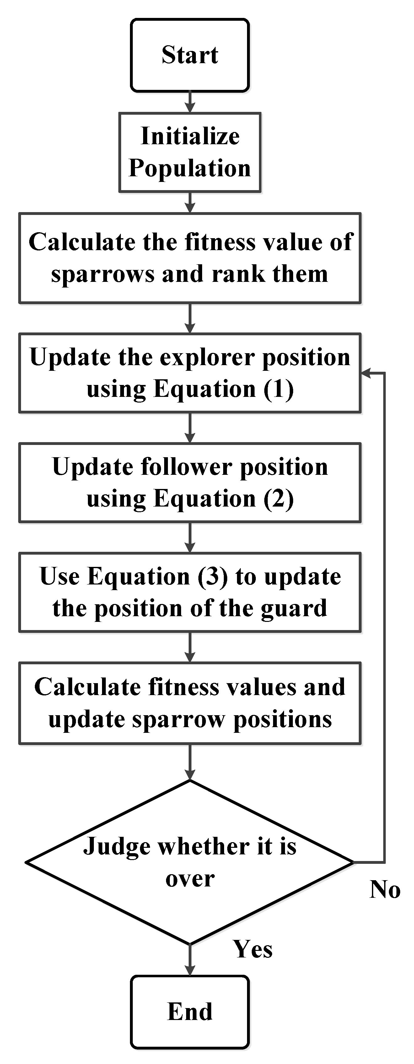
The SSA algorithm was proposed by Xue et al. [13] in 2020, analogizing the search process to that of a sparrow searching for food, which has the advantages of strong search ability and fast convergence. The algorithm divides sparrows into discoverers and followers by the level of fitness value: discoverers usually have high energy reserves and are responsible for providing areas and directions for followers; followers can always forage around discoverers that provide the best food or even directly take their place. Moreover, a certain number of vigilantes are set to prevent the search from falling into a local optimum. The explorer's location update formula is as follows:

$$X_{i,j}^{t+1}=\left\{\begin{array}{ll}{X}_{i,j}^t\cdot \exp \left(\frac{-i}{\alpha \cdot iter{}_{\max }}\right)\hfill & \mathrm{if}{R}_2<ST\hfill \\ X_{i,j}^t+Q\cdot \mathrm{L}\hfill & \mathrm{if}{R}_2\ge ST\hfill \end{array}\right.$$

(1)

where $X_{ij}$ is the position of each individual sparrow, $i$ is the number of current iterations, and $ite{r}_{\max }$ is the total number of iterations; α is a random number within [0, 1]; R₂ (R₂ ∈ [0, 1]), ST (ST ∈ [0.5, 1]) are the warning and safety values, respectively; Q is a random number obeying normal distribution; and L is a 1 × d matrix where each element is 1.

When the safety value of an individual sparrow is less than the warning value, that is, when R₂ < ST, it means that it is in a safe position at this time and the discoverer can maximize the global search. On the contrary, when R₂ > ST, some of the sparrows have found the danger and the followers have joined the action to monitor the discoverer, and once the discoverer has obtained a better value, it will take its place. The formula for updating the position of the followers is as follows:

$$X_{i,j}^{t+1}=\left\{\begin{array}{ll}Q\cdot \exp \left(\frac{X_{\mathrm{worst}}^t-X_{i,j}^t}{i^2}\right)\hfill & \mathrm{if}i>n/2\hfill \\ X_p^{t+1}+\left|X_{i,j}^t-X_P^{t+1}\right|\cdot A^{+}\cdot L\hfill & \mathrm{otherwise}\hfill \end{array}\right.$$

(2)

where n is the population size, $X_{\mathrm{worst}}$ is the position corresponding to the sparrow with the lowest global fitness, and $X_p$ is the position corresponding to the discoverer with the highest global fitness. A is a $1\times d$ matrix with random values of 1 or −1 for each element, where A⁺ is defined as $A^{+}=A^T{\left(A{A}^T\right)}^{-1}$.

Since each location update is followed by a ranking based on the fitness values of individual sparrows, $i>n/2$ means that some individuals with lower fitness are classified as followers with poorer status, and they cannot grab food from the discoverers and have to fly to other places to forage.

The sparrow algorithm defines 10–20% of individuals within the population as vigilantes in order to avoid falling into local optima when searching, and their initial positions are generated randomly with the position update formula shown below:

$$X_{i,j}^{t+1}=\left\{\begin{array}{ll}{X}_{\mathrm{best}}^t+\beta \cdot \left|X_{i,j}^t-X_{\mathrm{best}}^t\right|\hfill & \mathrm{if}{f}_i>f_g\hfill \\ X_{i,j}^t+K\cdot \left(\frac{\left|X_{i,j}^t-X_{\mathrm{worst}}^t\right|}{\left(f_i-f_w\right)+\epsilon }\right)\hfill & \mathrm{if}{f}_i=f_g\hfill \end{array}\right.$$

(3)

where $X_{\mathrm{best}}$ is the current global optimal position, β is the step control parameter, whose value is a random number obeying a normal distribution with mean 0 and variance 1; K is a random number within [−1, 1]; f is the fitness value, $f_g$ and $f_w$ are the current optimal and worst fitness values, respectively; ε is a constant to avoid the denominator being zero.

When $f_i>f_g$, this sparrow is less updated than the optimal value and is at the edge of the population and needs to move closer to the center of the population, while when $f_i=f_g$, it means that the sparrow in the middle of the population is aware of the danger and needs to find other sparrows to avoid being predated, that is, to fall into the local optimum. Here, K is the same as β and is also a step control parameter, which also indicates the direction of its movement. The steps of the traditional sparrow algorithm are as follows:

Step 1: Initialization: population number N, dimension D, discoverer proportion PD, vigilant proportion SD, warning value ST, initial value upper bound $ub$, lower bound $lb$, maximum number of iterations $T_{\max }$;

Step 2: Initialize the population;

Step 3: calculate the fitness values of sparrows and rand them;

Step 4: Update the discoverer position using Equation (1);

Step 5: Update the follower positions using Equation (2);

Step 6: Update the vigilantes’ positions using Equation (3);

Step 7: Calculate the fitness value and update the sparrow position;

Step 8: If the stop condition is satisfied, exit and output the result; otherwise, repeat Step 4.

The flow chart of traditional SSA is shown in Figure 1.

Traditional SSA also has some problems, such as random generation of initial individuals, which leads to insufficient population diversity; difficulty in balanced search and exploitation in discoverer location update, insufficient global search and local exploitation ability, and easy-to-fall-into local optimum. Therefore, some improvements are needed.

2.2. Improved SSA

To address the problems of traditional SSA mentioned above, the algorithm is improved by introducing tent chaotic mapping to initialize the population to improve the diversity of the population, improving the discoverer position update formula to balance its search and exploitation ability with the help of golden partition, and finally, introducing Gauss–Cauchy variation strategy to help ISSA jump out of local optimum. The improvement details are as follows.

2.2.1. Tent Chaotic Mapping Initializes the Population

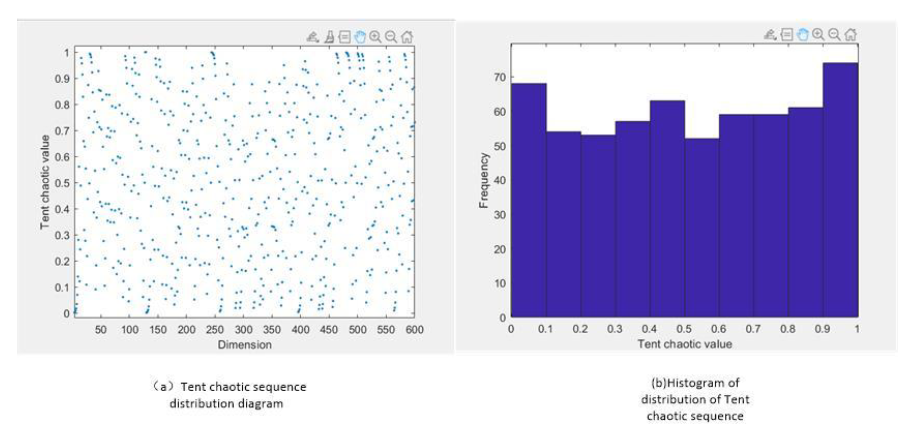
Based on the three main properties of chaotic variables, i.e., ergodicity, regularity and randomness, the global search capability of the algorithm is enhanced by preventing the algorithm from falling into a local optimum through its randomness while ensuring the diversity of the population. The expression of the tent mapping is shown in Equation (4).

$$z_{i+1}=\left\{\begin{array}{ll}2z_i& 0\le z\le \frac{1}{2}\\ 2(1-z_i)& \frac{1}{2}<z\le 1\end{array}\right.$$

(4)

where z is a random point between [0, 1]. i is the number of current iterations. The expression after Bernoulli transform is Equation (5).

$$z_{i+1}=(2z_i)\mathrm{mod}1$$

(5)

In order to avoid the existence of small cycles and unstable points in chaotic mapping and to preserve the periodicity, ergodicity, and regularity of chaotic variables, Wang et al. [20], based on the improved tent chaotic universal gravity search algorithm, added a random variable to the original expression, and the improved formula is given in Equation (6).

$$z_{i+1}=\left\{\begin{array}{ll}2z_i+\mathrm{rand}(0,1)\cdot \frac{1}{N_T}& 0\le z\le \frac{1}{2}\\ 2(1-z_i)+\mathrm{rand}(0,1)\cdot \frac{1}{N_T}& \frac{1}{2}<z\le 1\end{array}\right.$$

(6)

The expression after Bernoulli transform is given in Equation (7).

$$z_{i+1}=(2z_i)\mathrm{mod}1+\mathrm{rand}(0,1)\cdot \frac{1}{N_T}$$

(7)

where rand(0, 1) is a random number between [0, 1]. N_T is the number of particles in the chaotic sequence.

The distribution and histogram of 600 generations of improved tent chaos mapping are generated on MATLAB as shown in Figure 2.

As can be seen from Figure 2 the improved tent chaotic sequence is uniformly distributed between [0 and 1] and has good ergodicity. Finally, the initialized Tent chaotic population is obtained according to the upper and lower bounds of the given solution as shown in Equation (8).

$$X_{i,j}^{t+1}=lb+(ub-lb)Z_j$$

(8)

where lb is the lower bound of the solution space. ub is the upper bound of the solution space. Z_j is a j-dimensional sequence of tent chaos generated according to Equation (7).

2.2.2. Explorer Location Update Improvements

Golden-Sine is a new heuristic algorithm proposed by Tanyildizi et al. [21], which is inspired by the sine function and based on the relationship between the sine function and the unit circle. All values on the sine function can be traversed, i.e., all points on the unit circle can be searched, in order to scan the region that may yield only good results, largely improving the search speed and achieving a good balance between search and exploitation.

To address the problem that the discoverer position update process is difficult to balance search and exploitation, the optimization of the discoverer position update formula is considered. In the common discoverer position update formula, when the discoverer warning value is less than the safety value, the golden sine is introduced to replace the exponential random number, and the advantage of good traversal of the golden sine is used to reduce the solution space, improve the search speed, and balance the search and exploitation relationship between the two. The improved discoverer position update formula is shown in Equation (9).

$$X_{i,j}^{t+1}=\left\{\begin{array}{l}{X}_{i,j}^t\times \left|\sin (R_1)\right|+R_2\times \sin \left(R_1\right)\times \left|x_1\times X_{\mathrm{best}}^t-x_2\times X_{i,j}^t\right|R_2<ST\\ X_{i,j}^t+Q\cdot L{R}_2\ge ST\end{array}\right.$$

(9)

where R₁ is a random number that determines the distance an individual will move in the next iteration, taking values between [0, 2π]. R₂ determines the direction of the position update for the ith individual of the next iteration, taking values between [0, π]. x₁ and x₂ are coefficients obtained by introducing the golden mean, these coefficients narrow the search space, leading individuals to gradually converge to the optimal value, ensuring the convergence of the algorithm, the golden mean is related to the definition shown in Equation (10).

$$\left\{\begin{array}{l}{x}_1=a\tau +b(1-\tau )\\ x_2=a(1-\tau )+b\tau \\ \\ \tau =\frac{\sqrt{5}-1}{2}\end{array}\right.$$

(10)

where (a) the initial value is set to −π, and thereafter varies edge to edge as the target value changes; (b) the initial value is set to π, and thereafter the side changes as the target value changes.

2.2.3. Introduction of Gauss–Cauchy Mutation Strategy

The standard SSA algorithm late sparrow individuals assimilate rapidly, and there is a problem of local optimum stagnation that, combined with the characteristics of the normal distribution, can be seen. Gaussian mutation tends to focus on a local region of the original individual attachment, its local search ability is strong and good at solving optimization problems with a large number of local minimum values. The Gauss distribution function at the origin of the peak is relatively small but the distribution at both ends is relatively long, the use of its characteristics of the Cauchy mutation can generate larger perturbations in the individual attachment, making its ability to jump out of the local optimum enhanced. By introducing the Gaussian mutation operator and the Cauchy mutation operator [22], the fitness value f_i and the average fitness value f_avg of each sparrow are recalculated after one iteration of the sparrow algorithm is completed, i.e., the positions of the discoverers, followers and watchmen have been updated, and the better position before and after mutation is selected by the fitness selection mutation strategy and brought into the next iteration meritively without increasing the time complexity of the algorithm. The specific position update formula is shown in (11).

$$\left\{\begin{array}{l}{X}_{i,d}^{t+1}=X_{i,d}^t(1+{\lambda }_1\mathrm{Gauss}(0,1))f_i<f_{\mathrm{avg}}\\ X_{i,d}^{t+1}=X_{i,d}^t(1+{\lambda }_2\mathrm{cauchy}(0,1))f_i\ge f_{\mathrm{avg}}\end{array}\right.$$

(11)

where Gauss(0, 1) is a random variable satisfying the Gaussian distribution. Cauchy(0, 1) is a random variable satisfying the Cauchy distribution. λ₁ is a dynamic parameter that adaptively adjusts with the number of iterations ${\lambda }_1=1-\frac{t^2}{T_{\max }^2}$, λ₂ is a dynamic parameter that adaptively adjusts with the number of iterations ${\lambda }_2=\frac{t^2}{T_{\max }^2}$. t is the number of current iterations. T_max is the total number of iterations.

In the whole process of the optimization search: λ₁ gradually decreases and λ₂ gradually increases, the Gaussian mutation dominates at the beginning of the iteration for enhancing the local search ability, focusing on solving the optimization problem of local minimum values and enhancing the robustness of the algorithm to a certain extent; the late iteration mainly helps the individual to jump out of the local optimum through the Cauchy variation so that it can better reach the global optimum.

2.2.4. ISSA Implementation Steps and Flow Chart

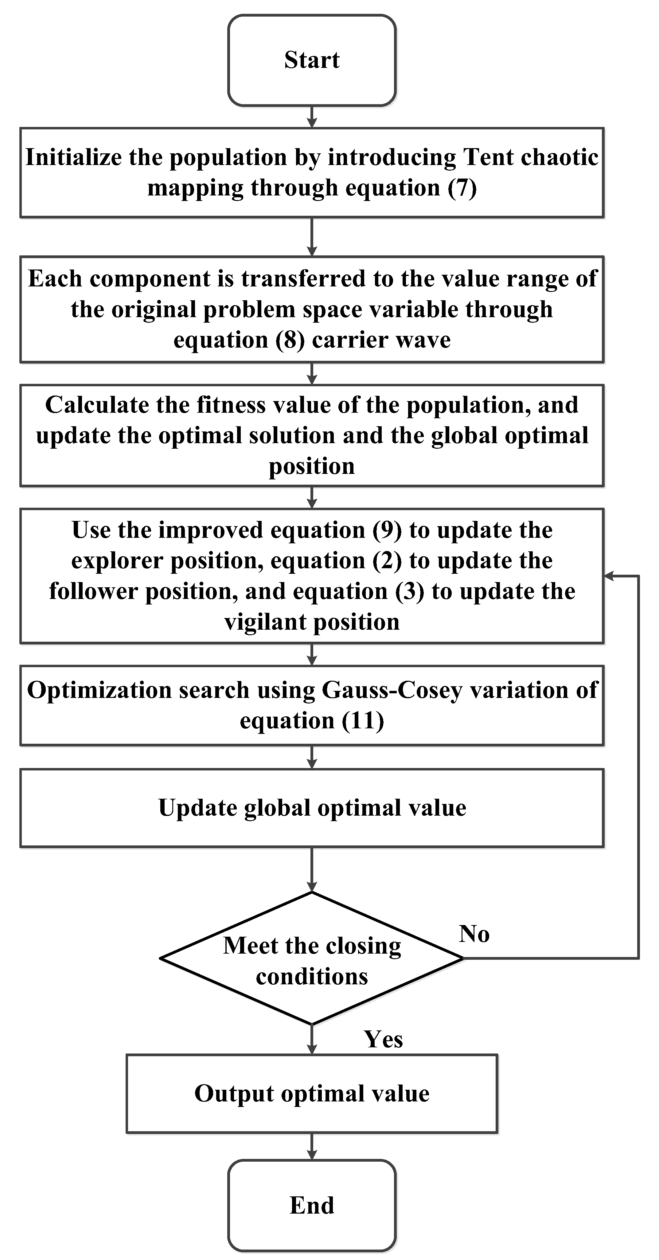
The ISSA algorithm introduces tent chaotic mapping to initialize the population, which increases the diversity of the population, introduces golden sine to improve the discoverer position update formula, which balances the search performance of the algorithm with the pioneering performances, and introduces the Gauss–Cauchy variation strategy to help the algorithm jump out of the local optimum. Its concrete implementation steps are as follows:

Step 1: Initialization: population number n, dimension D, discoverer proportion PD, vigilant proportion SD, warning value ST, initial value upper bound $ub$, lower bound $lb$, maximum number of iterations $T_{\max }$;

Step 2: Initialize the population by the Tent chaotic sequence in Equation (7), generate N D-dimensional vectors $Z_i$, and carrier its components into the range of values of the original problems space variables by Equation (8);

Step 3: Calculate the fitness f_i of each sparrow and select the current optimal fitness value $f_g$ and its corresponding position $x_b$;

Step 4: Select the top $P_{Num}$ sparrows with good adaptation as discoverers and the rest as followers, update the discoverer positions according to the discoverer position update Equation (9) after introducing the golden mean, and update the follower positions according to Equation (2);

Step 5: Randomly select $S_{Num}$ sparrows from the sparrow population as vigilantes and update their positions according to Equation (3);

Step 6: After one iteration, recalculate the fitness value f_i for each sparrow and the average fitness value $f_{\mathrm{avg}}$ for the sparrow population;

(1) When $f_i<f_{\mathrm{avg}}$ indicates the phenomenon of “aggregation”, Gaussian variation is performed according to Equation (11), and if the mutated individual is better, it replaces the one before the mutation, otherwise it remains unchanged.

(2) When $f_i\ge f_{\mathrm{avg}}$ indicates a trend of “divergence”, we will carry out the Cauchy variation according to Equation (11), and replace the individuals before the variation if they are better after the variation, otherwise, they will remain unchanged.

Step 7: Based on the current state of the sparrow population, update the optimal position $x_b$ experienced by the entire population and its fitness value $f_g$;

Step 8: Determine whether the operation of the algorithm meets the stopping condition, if it does, exit and output the result, otherwise, repeat to step 4.

The flow chart of ISSA is shown in Figure 3.

3. Performance Analysis on Benchmark Functions

3.1. Selection of Test Functions

In order to verify the feasibility of the improved sparrow algorithm, 30 different types of test functions [23] were selected for simulation experiments to examine the full range of the improved sparrow algorithm’s optimization-seeking ability through different types of functions. Among them, F₁ to F₇ are unimodal test functions; F₈ to F₁₃ are high-dimensional multimodal test functions; F₁₄ to F₂₃ are fixed-dimensional multimodal test functions; and F₂₄ to F₃₀ are complex test functions. As shown in

Table 1. Test function.

Type	Function Name	Dimensionality	Search Space	Optimum Value
High-dimensional unimodal	Sphere(F1)	30	[−100, 100]	0
	Schwefel 2.22(F2)	30	[−10, 10]	0
	Schwefel 1.2(F3)	30	[−100, 100]	0
	Schwefel 2.21(F4)	30	[−100, 100]	0
	Generalized Rosenbrock(F5)	30	[−30, 30]	0
	Step Function(F6)	30	[−100, 100]	0
	Quartic(F7)	30	[−1.28, 1.28]	0
High-dimensional multimodal	Schwefel2.26(F8)	30	[−500, 500]	−12,569.5
	Rastrigin(F9)	30	[−5.12, 5.12]	0
	Ackley(F10)	30	[−32, 32]	0
	Griewank(F11)	30	[−600, 600]	0
	Generalized Penalized Function 1(F12)	30	[−50, 50]	0
	Generalized Penalized Function 2(F13)	30	[−50, 50]	0
Fixed-dimension multimodal	Shekel's Foxholes(F14)	2	[−65.53, 65.53]	1
	Kowalik(F15)	4	[−5, 5]	0.0003075
	Six-Hump Camel-Back(F16)	2	[−5, 5]	−1.031628
	Branin(F17)	2	lb = [−5, 0] ub = [10, 15]	0.398
	Goldstein-Price(F18)	2	[−2, 2]	3
	Hartman's Family n = 3(F19)	3	[0, 1]	−3.98
	Hartman's Family n = 6(F20)	6	[0, 1]	−3.32
	Shekel's Family m = 5(F21)	4	[0, 10]	−10.536
	Shekel's Family m = 7(F22)	4	[0, 10]	−10.536
	Shekel's Family m = 10(F23)	4	[0, 10]	−10.536
Complicated	Eggholder(F24)	2	[−512, 512]	−959.6407
	Holder Table(F25)	2	[−10, 10]	−19.2085
	Langermann(F26)	2	[0, 10]	−4.1558
	Levy N.13(F27)	2	[−10, 10]	0
	Michalewicz(F28)	10	[0, π]	−9.66015
	Three-Hump Camel(F29)	2	[−5, 5]	0
	Perm Function 0, d, β(F30)	10	[−10, 10]	0

.

3.2. Experimental Environment and Comparison Algorithm Selection

The experiments were conducted in AMD Ryzen 7 5800H [email protected] GHz, 16.00 GB of memory, Windows 10 system and MATLAB R2020. The original Sparrow Search Algorithm (SSA), Improved Sparrow Search Algorithm (ISSA), Grey Wolf Optimization Algorithm [24] (GWO), particle swarm algorithm [25,26] (PSO) and Moth-Flame Optimization Algorithm [27] (MFO) for the comparison test of the test functions.

Among them, the selection of each comparison algorithm is based on the following bases: SSA is the original algorithm of ISSA; GWO has a strong search capability and it is easy to find the optimal value of the test function, which is used to focus on comparing the ability of ISSA to find the optimal solution; PSO has a simple structure and short running time in the search process, which is used to focus on comparing the stability and real-time performances of ISSA in the search process; MFO can widely explore the search space. It is easier to find the global optimal solution, and it is used to focus on comparing the ability of ISSA to jump out of the local optimum.

3.3. Comparative Analysis of Performance Indicators

In the experiment, the population size N = 30, the maximum number of iterations $ite{r}_{\max }=500$, the dimensionality of the objective function D and the initial values of the upper and lower bounds $ub$ and $lb$ are shown in Table 1, and the number of discoverers PD and the number of watchmen SD are taken as 20% of the total population size. In order to avoid the chance of the search results for the test functions, the experimental results of 30 independent runs of each benchmark test function were selected as the experimental data. The mean, standard deviation, optimal value and the number of iterations of the search results for the 30 test functions were used as the final performance evaluation indexes, as shown in

Table 2. Optimal value of test function search results.

Type	Function	GWO	PSO	MFO	SSA	ISSA
High-dimensional unimodal	F1	1.071 × 10−27	334.718	2.071	4.821 × 10−98	6.15 × 10−145
	F2	1.054 × 10−18	15.051	30.111	1.232 × 10−42	1.633 × 10−43
	F3	1.212 × 10−8	5.105 × 103	2.037 × 104	1.054 × 10−27	3.549 × 10−34
	F4	4.282 × 10−7	6.821	70.487	5.355 × 10−29	1.091 × 10−50
	F5	0.446	1.101 × 104	1.919 × 103	6.978 × 10−5	1.076 × 10−7
	F6	0.504	355.921	990.794	3.324 × 10−6	1.339 × 10−12
	F7	1.300 × 10−3	0.535	2.528	1.200 × 10−3	6.225 × 10−5
High-dimensional multimodal	F8	−9.70 × 103	−6.266 × 103	−4.05 × 103	−1.25 × 104	−1.25 × 104
	F9	0	1.0267 × 102	1.550 × 102	0	0
	F10	8.882 × 10−16	4.5047	5.393	8.882 × 10−16	8.882 × 10−16
	F11	0.001	0	4.931	0	0
	F12	0.033	5.647	32.821	1.050 × 10−7	2.233 × 10−13
	F13	0.616	9.983	6.258	9.574 × 10−9	4.573 × 10−14
Fixed-dimension multimodal	F14	2.9821	1.003	0.998	2.982	0.998
	F15	3.378 × 10−4	0.023	7.837 × 10−4	3.378 × 10−4	3.132 × 10−4
	F16	−1.032	−1.032	−1.032	−1.032	−1.032
	F17	0.398	0.398	0.398	0.398	0.398
	F18	3.000	3.002	3.000	3.002	3.000
	F19	−3.863	−3.863	−3.863	−3.863	−3.863
	F20	−3.322	−3.326	−3.203	−3.231	3.322
	F21	−9.392	−10.154	−10.055	−10.153	−10.536
	F22	−10.403	−10.403	−10.403	−10.403	−10.403
	F23	−10.535	−10.536	−10.536	−10.536	−10.536
Complicated	F24	−959.6407	−959.6407	−959.6407	−959.6407	−959.6407
	F25	−19.2085	−19.2085	−19.2085	−19.2085	−19.2085
	F26	−4.1558	−4.1558	−4.1558	−4.1558	−4.1558
	F27	8.588 × 10−8	7.570 × 10−6	1.348 × 10−31	1.459 × 10−8	1.348 × 10−31
	F28	−8.946	−6.874	−9.005	−8.454	−9.552
	F29	1.48 × 10−199	1.248 × 10−5	6.92 × 10−110	3.275 × 10−64	1.94 × 10−179
	F30	0.103	17.276	1.033 × 10−6	0.002	0.116

,

Table 3. Mean value of test function search results.

Type	Function	GWO	PSO	MFO	SSA	ISSA
High-Dimensional unimodal	F1	1.153 × 10−27	3.786 × 102	2.781	2.696 × 10−63	9.855 × 10−95
	F2	8.864 × 10−17	18.415	38.778	7.844 × 10−32	1.690 × 10−46
	F3	8.906 × 10−6	7.740 × 103	2.164 × 104	2.554 × 10−27	3.286 × 10−31
	F4	6.657 × 10−7	9.728	68.5053	9.456 × 10−15	3.15 × 10−27
	F5	0.7904	1.687 × 104	8.017 × 106	8.807 × 10−4	1.17 × 10−4
	F6	0.6316	359.709	3.332 × 103	5.493 × 10−6	7.84 × 10−12
	F7	1.900 × 10−3	0.987	2.730	1.700 × 10−3	5.774 × 10−4
High-dimensional multimodal	F8	−5.74 × 103	−7.376 × 103	−4.08 × 103	−8.48 × 103	−1.15 × 104
	F9	2.838	1.943 × 102	1.578 × 102	0	0
	F10	9.883 × 10−14	5.899	14.859	8.882 × 10−16	8.882 × 10−16
	F11	0.002	3.834	30.969	0	0
	F12	0.047	5.802	639.216	2.884 × 10−7	4.10 × 10−12
	F13	0.706	22.964	39.506	8.27 × 10−6	4.40 × 10−12
Fixed-dimension multimodal	F14	3.515	1.040	1.757	5.349	1.004
	F15	0.006	0.008	0.001	4.038 × 10−4	3.20 × 10−4
	F16	−1.032	−1.032	−1.032	−1.032	−1.032
	F17	0.398	0.398	0.398	0.398	0.398
	F18	5.700	3.002	3.000	3.900	3.000
	F19	−3.862	−3.860	−3.863	−3.863	−3.863
	F20	−3.264	−3.091	−3.236	−3.251	−3.296
	F21	−9.317	−9.802	−8.418	−8.914	−10.532
	F22	−10.225	−9.706	−8.762	−9.163	−10.397
	F23	−10.264	−10.264	−8.383	−8.914	−10.530
Complicated	F24	−868.854	−926.734	−931.834	−917.836	−959.488
	F25	−19.2085	−18.504	−20.584	−19.0125	−19.2085
	F26	−4.0326	−3.7992	−4.0148	−4.1288	−4.1342
	F27	4.006 × 10−7	1.059 × 10−4	1.348 × 10−31	7.522 × 10−6	1.348 × 10−31
	F28	−7.854	−5.729	−7.796	−7.981	−8.011
	F29	6.9 × 10−189	3.365 × 10−6	1.30 × 10−103	2.637 × 10−35	3.9 × 10−169
	F30	8.636	152.489	9.240	10.899	7.639

,

Table 4. Variance of test function search results.

Type	Function	GWO	PSO	MFO	SSA	ISSA
High-dimensional unimodal	F1	2.942 × 10−27	1.708 × 102	2.000	1.196 × 10−62	2.203 × 10−94
	F2	5.698 × 10−17	12.794	20.239	3.778 × 10−31	3.778 × 10−46
	F3	1.832 × 10−5	5.881 × 103	1.124 × 104	1.376 × 10−26	9.735 × 10−31
	F4	5.501 × 10−7	2.718	7.814	5.180 × 10−14	1.67 × 10−26
	F5	0.7904	1.392 × 104	3.218 × 107	0.001	3.82 × 10−4
	F6	0.372	216.624	6.600 × 103	1.043 × 10−5	2.01 × 10−11
	F7	9.494 × 10−4	2.723	6.149	1.400 × 10−3	2.239 × 10−4
High-dimensional multimodal	F8	1.036 × 103	1.069 × 103	8.103 × 102	5.312 × 103	1.644 × 103
	F9	4.348	30.75	33.111	0	0
	F10	1.552 × 10−14	0.883	6.985	0	0
	F11	0.006	1.372	49.146	0	0
	F12	0.024	3.171	3.438 × 103	5.684 × 10−7	1.53 × 10−11
	F13	0.2384	14.699	77.229	1.423 × 10−5	7.12 × 10−12
Fixed-dimension multimodal	F14	3.801	0.1123	1.365	5.454	1.680 × 10−2
	F15	0.009	0.009	0.001	2.935 × 10−4	2.874 × 10−4
	F16	1.802 × 10−8	2.250 × 10−5	6.775 × 10−16	2.003 × 10−5	5.04 × 10−16
	F17	7.534 × 10−5	9.261 × 10−6	0	3.325 × 10−5	0
	F18	14.788	1.68 × 10−4	6.696 × 10−4	4.929	1.92 × 10−15
	F19	0.002	0.004	0.001	6.872 × 10−4	2.30 × 10−15
	F20	0.091	0.181	0.059	0.059	0.052
	F21	2.210	2.139	3.575	2.521	5.700 × 10−3
	F22	0.963	1.878	3.052	2.287	0.006
	F23	1.481	1.250	3.386	2.520	0.013
Complicated	F24	90.299	33.497	44.750	45.879	0.835
	F25	2.241 × 10−5	1.231	1.426	0.746	7.58 × 10−15
	F26	0.204	0.665	0.183	0.005	0.012
	F27	3.514 × 10−7	1.338 × 10−4	6.68 × 10−47	1.646 × 10−5	6.68 × 10−47
	F28	1.129	0.838	0.909	0.809	0.781
	F29	0	4.818 × 10−6	7.02 × 10−103	1.444 × 10−34	0
	F30	11.406	120.335	9.075	11.134	8.950

and

Table 5. Number of iterations to test the optimization results of the function.

Type	Function	GWO	PSO	MFO	SSA	ISSA
High-dimensional unimodal	F1	500	500	500	500	283
	F2	500	500	500	500	408
	F3	500	500	500	500	452
	F4	500	500	500	430	287
	F5	56	500	500	500	34
	F6	500	500	500	500	500
	F7	267	383	390	500	172
High-dimensional multimodal	F8	500	500	190	112	201
	F9	500	500	500	72	18
	F10	368	500	500	278	85
	F11	180	189	500	64	27
	F12	500	500	500	500	283
	F13	500	500	500	500	500
Fixed-dimension multimodal	F14	83	59	29	77	6
	F15	500	500	500	500	500
	F16	4	1	1	2	1
	F17	115	92	13	28	8
	F18	36	73	38	8	6
	F19	199	90	17	24	7
	F20	196	500	500	17	8
	F21	434	202	32	423	7
	F22	298	500	46	448	10
	F23	457	266	47	500	29
Complicated	F24	35	500	22	500	13
	F25	24	8	32	3	1
	F26	40	7	80	15	12
	F27	500	500	172	116	500
	F28	500	500	151	390	137
	F29	500	500	500	500	500
	F30	500	500	500	500	500

, where the bolded items are the optimal indexes of the same test function.

Analyzing Table 2, Table 3, Table 4 and Table 5, we can see that based on the same constraints, for the functions F₁–F₃₀, the mean and standard deviation of ISSA are significantly better than the other four comparative optimization algorithms, and for different test functions, ISSA can find its optimal value within 30 times and the number of its iterations to find the optimal value is much lower than the other algorithms. Among them, for the high-dimensional single-peak functions: for the functions F₁–F₇, the average value of ISSA is closer to the optimal value, and the standard deviation is much lower than other algorithms, especially for the functions F₁–F₄, the order of magnitude of the search results is improved by at least 19 orders of magnitude compared with traditional SSA, which indicates that the accuracy and stability of its search are greatly improved. For functions F₅–F₇, although the improvement of the optimization results is not obvious, it is also significantly better than other comparative algorithms. For high-dimensional multimodal, for the functions F₈–F₁₁, ISSA and SSA can find the optimal solution compared with other algorithms, but the mean and variance of ISSA are smaller, which indicates that the superiority of the improved algorithm itself is not destroyed, and the stability is stronger. For functions F₁₂ and F₁₃, although the iteration time is longer and the optimal solution of the test function is not found for 500 iterations, the optimal value, mean and variance are better than the other compared algorithms. For fixed-dimensional multi-peak functions, among the 10 test functions, the number of functions for which ISSA, SSA, GWO, MFO and PSO can find the optimal solution among the 10 test functions are 9, 5, 5, 8 and 5, respectively, and the number of optimal values for 30 times are 5, 3, 2, 4 and 2, respectively, and the variance of ISSA is the smallest for all 30 times of finding the optimal value, and ISSA is much better than other algorithms in the performance of fixed-dimensional multi-peak test functions. For complex test functions, for functions F₂₆–F₂₈, all five algorithms can find their optimal values, but the mean and variance of ISSA are lower, except for F₂₈, which has a higher number of iterations than SSA, and all others are lower than the other algorithms. For function F₂₉, the optimal value and mean performance are not as good as GWO, the variance is the same, and the number of iterations is the same. For function F₃₀, except for the optimal value, which is not as good as MFO, all other performance indicators are better than the other algorithms. In summary, it can be seen that the ISSA algorithm outperforms all other algorithms in different types of 30 test functions, except for individual test functions that are inferior to individual algorithms, proving the excellent performance of the improved sparrow search algorithm.

3.4. Running Time Comparison Analysis

Real-time performance is an important index to evaluate the superiority of the algorithm, and the average running time of ISSA and SSA for 30 times of optimization of different test functions is experimentally derived. The running time comparison results are shown in

Table 6. Comparison of the running time of test functions by the sparrow algorithm before and after improvement.

Type	Function	SSA	ISSA
		Mean Running Time/s
High-dimensional unimodal	F1	0.2940	0.1937
	F2	0.3895	0.3963
	F3	0.5226	0.5129
	F4	0.3578	0.3485
	F5	0.3872	0.3439
	F6	0.3287	0.3443
	F7	0.4786	0.4425
High- dimensional multimodal	F8	0.4175	0.4132
	F9	0.3989	0.3911
	F10	0.3848	0.4037
	F11	0.4194	0.4225
	F12	0.3849	0.3389
	F13	0.3525	0.3361
Fixed-dimension multimodal	F14	0.7484	0.7105
	F15	0.1920	0.1474
	F16	0.1886	0.1810
	F17	0.1816	0.1721
	F18	0.1802	0.1699
	F19	0.2076	0.2157
	F20	0.2108	0.2434
	F21	0.2526	0.2298
	F22	0.2396	0.2694
	F23	0.2562	0.2964
Complicated	F24	0.1832	0.1694
	F25	0.1834	0.1681
	F26	0.2570	0.2865
	F27	0.1862	0.1754
	F28	0.3598	0.3436
	F29	0.1931	0.1886
	F30	1.1782	1.2938

.

From Table 6, it can be seen that the mean running time of ISSA on 20 out of 30 test functions is slightly better than that of the standard SSA, and the running time used on the other 10 test functions is approximately the same, which verifies the consistency in time complexity between the improved SSA and the standard SSA in this paper, and the improvement of the algorithm does not reduce the real-time performance while improving the performance.

3.5. Comparison of Convergence Curves of Fitness Values

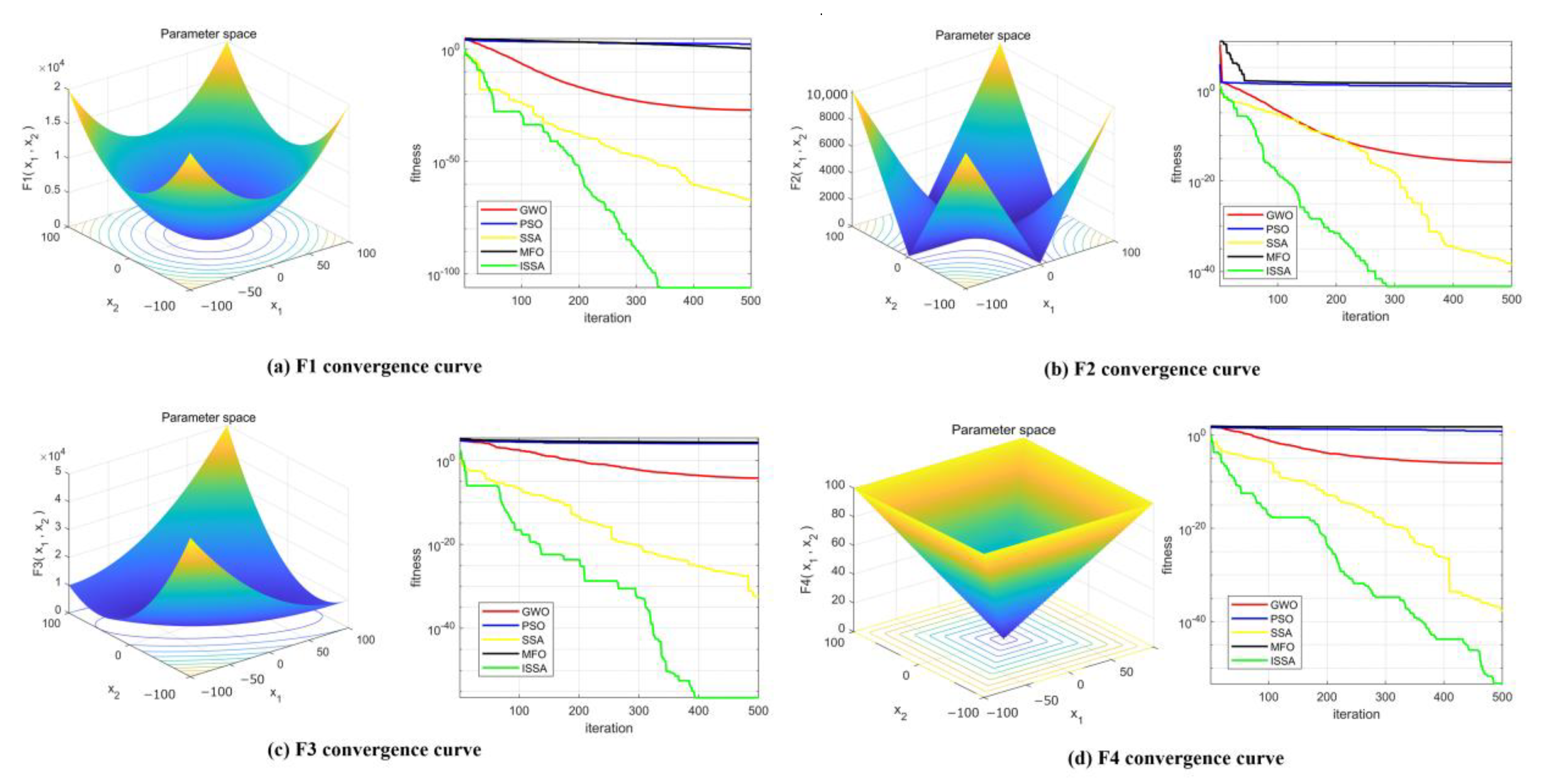
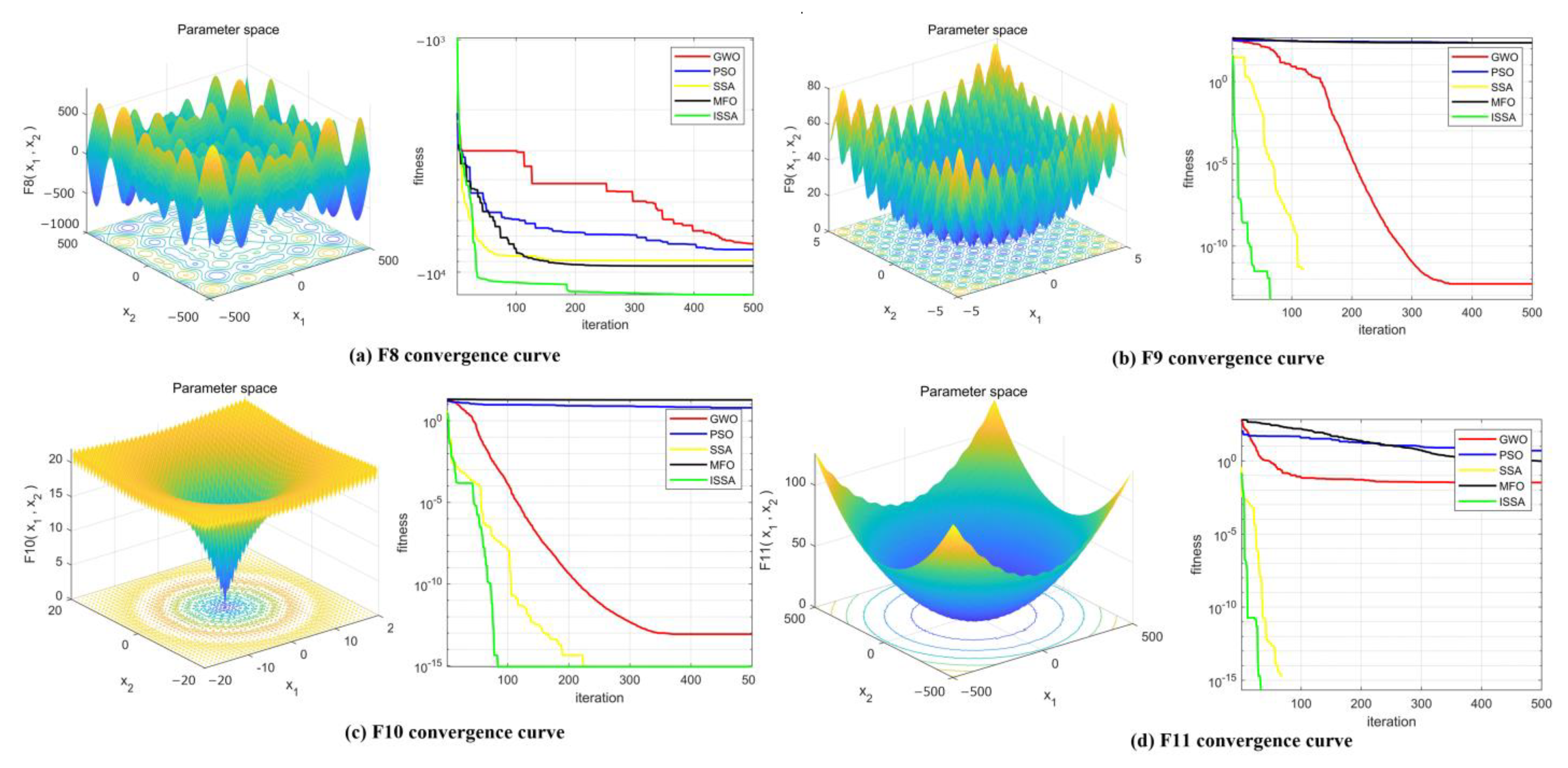
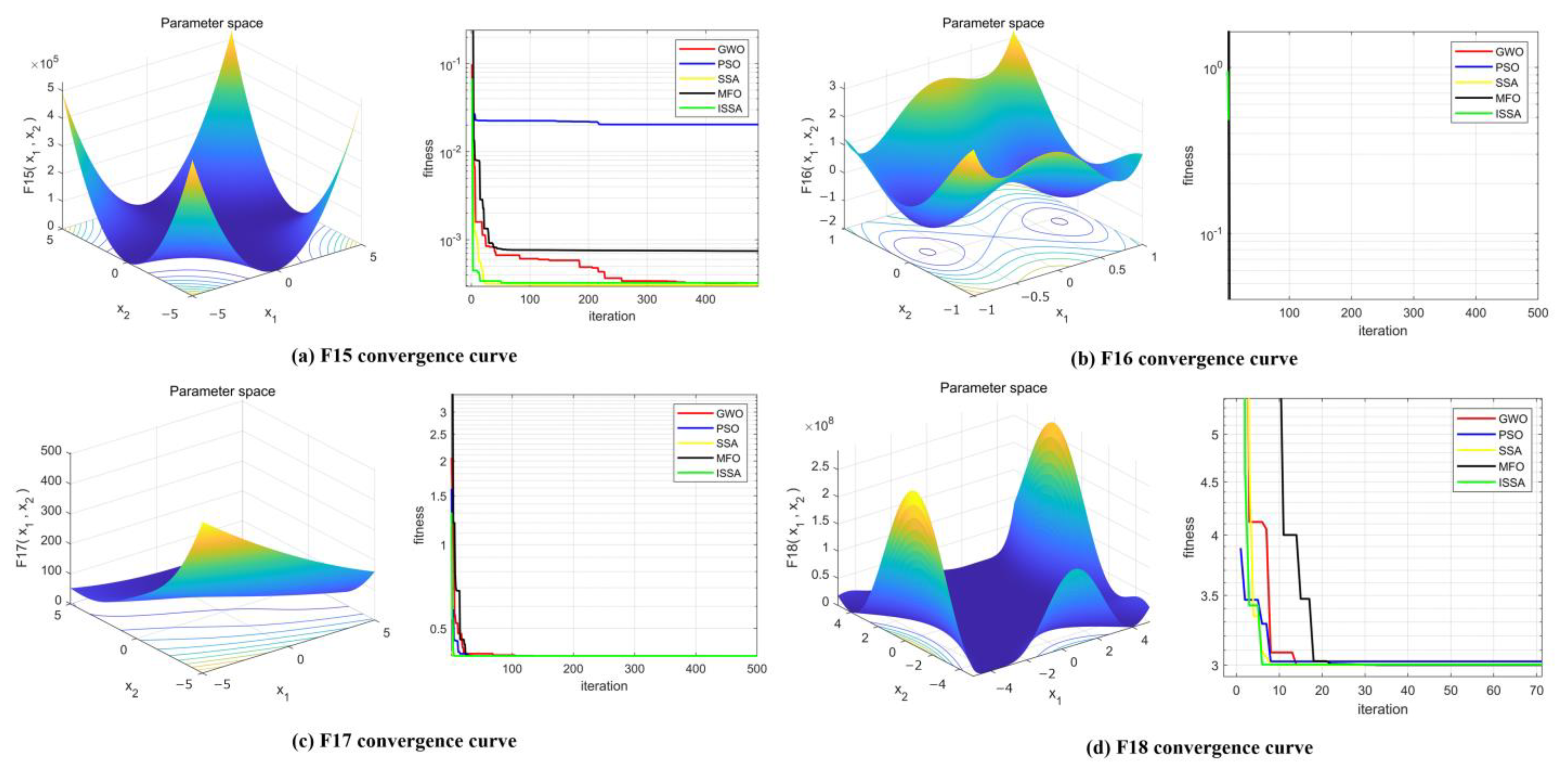
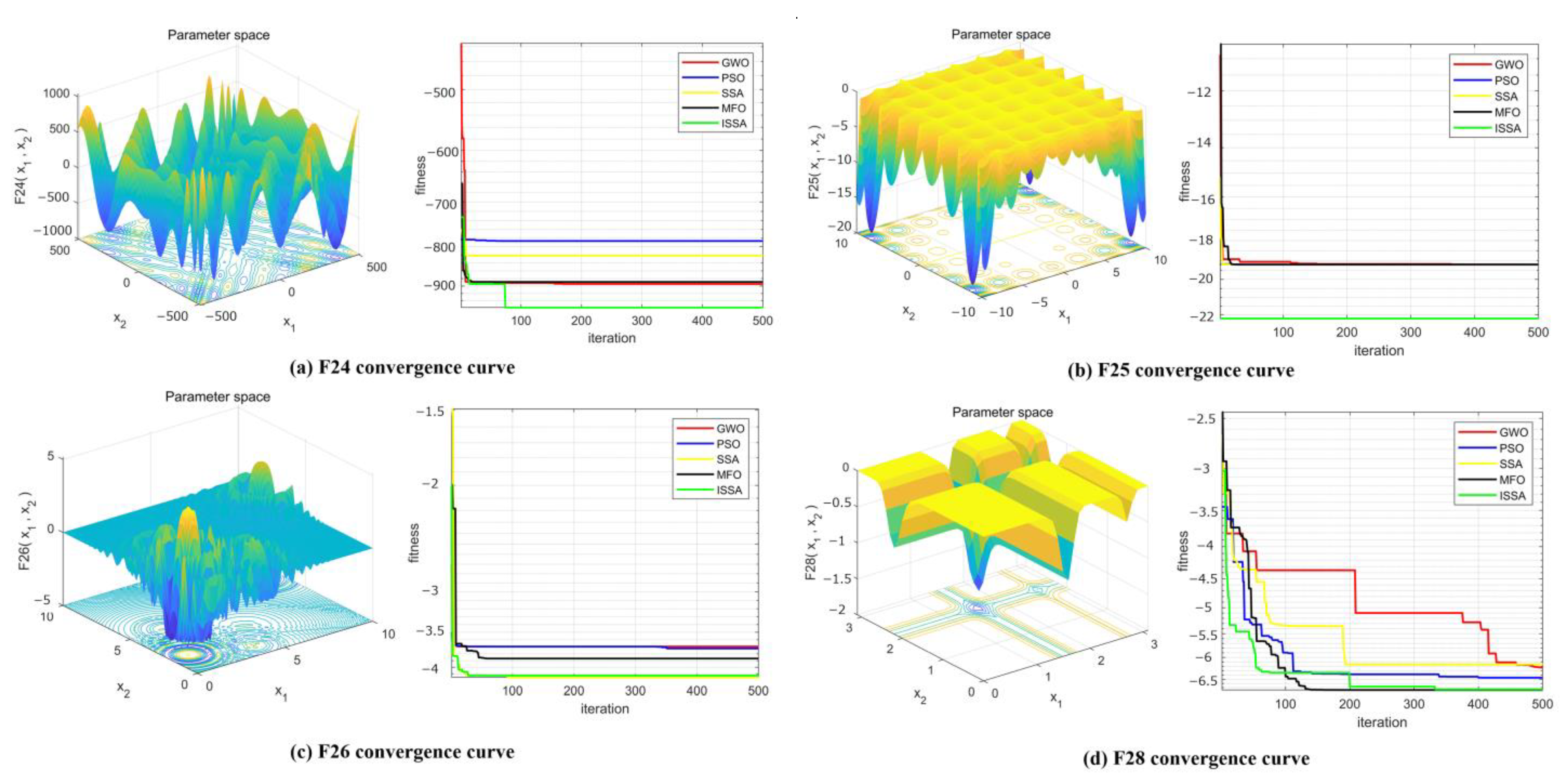
In order to reflect the dynamic convergence characteristics of ISSA and further visualize and compare the convergence of each algorithm and the ability to jump out of the local optimum, the convergence curves of four test functions of each type are given for a total of sixteen test functions under five optimization algorithms, where the horizontal coordinates are the number of iterations and the vertical coordinates are the values of the fitness functions. As shown in Figure 4, Figure 5, Figure 6 and Figure 7.

The analysis of Figure 4, Figure 5, Figure 6 and Figure 7 shows that for the functions F₁, F₂, F₃, F₄, F₈, F₂₄ and F_25, ISSA is far better than the other comparison algorithms in both convergence speed and search accuracy, an indication that the strategy of initializing the population by tent mapping effectively improves the diversity and pioneering of the population, and the golden sine strategy improves the discoverer search method to improve the global search ability of the algorithm. For the functions F₉, F₁₀, F₁₁, F₁₅, F_16, F₁₇, F₁₈ and F₂₆, although ISSA and other compared algorithms eventually converge to the optimal value, ISSA has fewer iterations and higher efficiency of the search. Although there is a tendency to fall into the local optimum in the late stage of the search, the Gauss–Cauchy variation strategy introduced by the algorithm effectively jumps out of the local optimum and converges to the global optimum. For function F₂₈, only ISSA and MFO eventually converge, but the number of ISSA iterations is slightly higher than that of MFO.

In summary, it can be seen that ISSA has significantly improved the search ability for different types of benchmark functions, whether it is a high-dimensional single-peak function, high-dimensional multi-peak function, fixed-dimensional multi-peak function or a more complex function than other comparison algorithms. At the same time, its fast convergence speed and short operation time can meet the demand for real-time algorithms and effectively avoid falling into local optimum while ensuring the search speed, thus proving the feasibility and superiority of ISSA.

4. Performance Analysis of Reactor Model for Temperature Control

4.1. Reactor Temperature Control System Model

4.1.1. Heat Exchanger Description

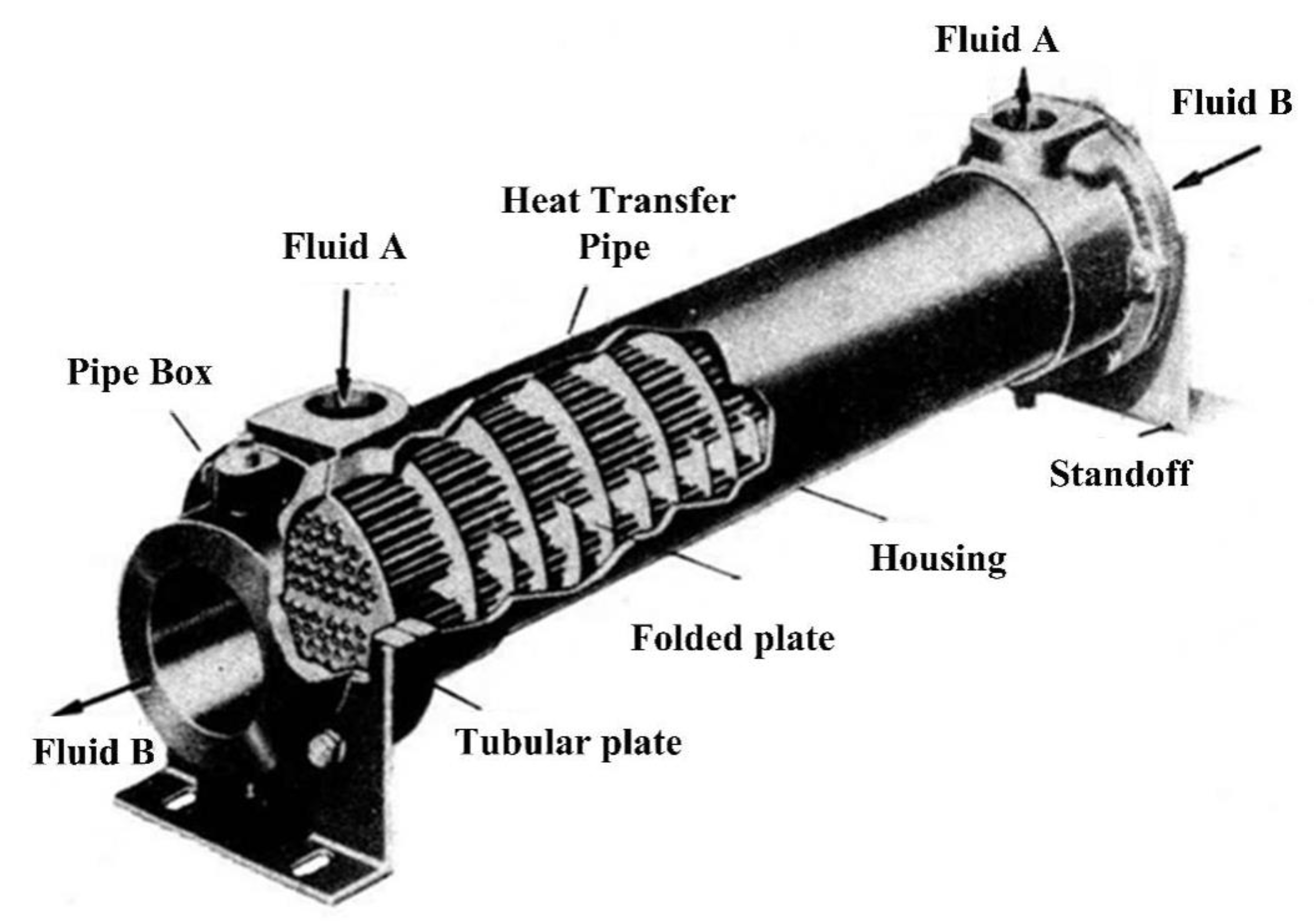
In the chemical production process, to obtain a high reaction rate, the reactor needs to be controlled near the optimal temperature, so for the exothermic reaction, generated heat energy needs to be offset, and the heat-absorbing reaction needs to be provided with sufficient heat energy, which uses a heat exchanger in order to maximize the contact area of heat transfer. The practical application of the general use of tubular heat exchangers, such as Figure 8, shows the structure of a heat exchanger, the heat exchanger through different temperatures of fluid through the shell process and the fluid in the tube process to complete the heat transfer.

The exit temperature of the heat exchanger is generally simplified to a second-order with a time lag model, which affects the exit temperature of the tube process by controlling the flow rate of the fluid in the shell process, while the control of the flow rate is controlled by the opening of the flow control valve of the inlet line of the circulating cooling water. Therefore, by controlling the regulating valve opening, the heat exchanger outlet temperature can be controlled.

4.1.2. Heat Exchanger Model Identification

Let the heat exchanger input be T₁₁F₁ and T₂₁F₂, and the output be T₂₂ and T₁₂, where the controlled variable is the heat exchanger output temperature T₁₂, and the control variable is the circulating cooling water flow rate F₂. It is assumed that there is no heat loss in the heat exchanger, the same heat transfer coefficient is K₁₂ and the fluid flow in the tube can always be controlled. The total set parameter model is used for mechanism modeling, and the heat exchanger outlet temperature T₁₂ is selected as the total set parameter and the fluid flow delay is considered for system modeling.

According to the energy dynamic balance, Equation (12) can be obtained:

$$\begin{array}{l}{M}_1{C}_1\frac{\mathrm{d}{T}_{12}}{\mathrm{d}t}=F_1{C}_1\left(T_{11}-T_{12}\right)+K_{12}A\left(T_{22}-T_{12}\right)\hfill \\ M_2{C}_2\frac{\mathrm{d}{T}_{22}}{\mathrm{d}t}=F_2{\mathrm{C}}_2\left(T_{21}-T_{22}\right)-K_{12}A\left(T_{22}-T_{12}\right)\hfill \end{array}$$

(12)

where $M_i$ is the corresponding fluid mass in the tube. C_i is the specific heat capacity of the corresponding fluid. A is the average thermal conductivity area. $T_i$ is the corresponding temperature. Simplifying and linearizing Equation (12), the state space model can be obtained as shown in Equation (13).

$$\dot{X}=\left[\begin{array}{ll}{a}_1\hfill & a_2\hfill \\ b_1\hfill & b_2\hfill \end{array}\right]X+\left[\begin{array}{cccc}{a}_3& 0& a_4& 0\\ 0& b_3& 0& b_4\end{array}\right]U$$

(13)

where $U={\left[\begin{array}{cccc}{T}_{11}& T_{21}& F_1& F_2\end{array}\right]}^{\mathrm{T}}$. $X={\left[\begin{array}{cc}{T}_{12}& T_{22}\end{array}\right]}^{\mathrm{T}}$. $a_1=-\left(\frac{{\overline{F}}_1}{M_1}+\frac{K_{12}A}{C_1{M}_1}\right)$. $a_2=\frac{K_{12}A}{C_1{M}_1}$. $a_3=\frac{{\overline{F}}_1}{M_1}$. $a_4=\frac{1}{M_1}\left({\overline{T}}_{11}-T_{12}\right)$. $b_1=\frac{K_{12}A}{C_2{M}_2}$. $b_2=-\left(\frac{{\overline{F}}_2}{M_2}+\frac{K_{12}A}{C_2{M}_2}\right)$. $b_3=\frac{{\overline{F}}_2}{M_2}$. $b_4=\frac{1}{M_2}\left({\overline{T}}_{21}-{\overline{T}}_{22}\right)$. In the Equation, the one with the “—” symbol indicates the steady-state value.

Transform Equation (13) into a transfer function as shown in Equation (14).

$$\left[\begin{array}{l}{T}_{12}\hfill \\ T_{22}\hfill \end{array}\right]=\frac{1}{\left(s-a_1\right)\left(s-a_2\right)-a_2{b}_1}\times {\left[\begin{array}{cc}\left(s-b_2\right)a_3& b_1{a}_3\\ a_2{b}_3& \left(s-a_2\right)b_3\\ \left(s-b_2\right)a_4& b_1{a}_4\\ a_2{b}_4& \left(s-a_2\right)b_4\end{array}\right]}^{\mathrm{T}}\left[\begin{array}{l}{T}_{11}\hfill \\ T_{21}\hfill \\ F_1\hfill \\ F_2\hfill \end{array}\right]$$

(14)

The control system transfer function is shown in Equation (15).

$$G(s)=\frac{T_{12}(s)}{F_2(s)}=\frac{a_2{b}_4}{\left(s-a_1\right)\left(s-a_2\right)-a_2{b}_1}$$

(15)

Considering the heat transfer delay, the heat exchanger is in the second-order with delay form as shown in Equation (16).

$$G(s)=\frac{K}{\left(T_{1}s+1\right)\left(T_{2}s+1\right)}{e}^{-\tau s}$$

(16)

where K is system gain. T is the time constant. τ is the delay time.

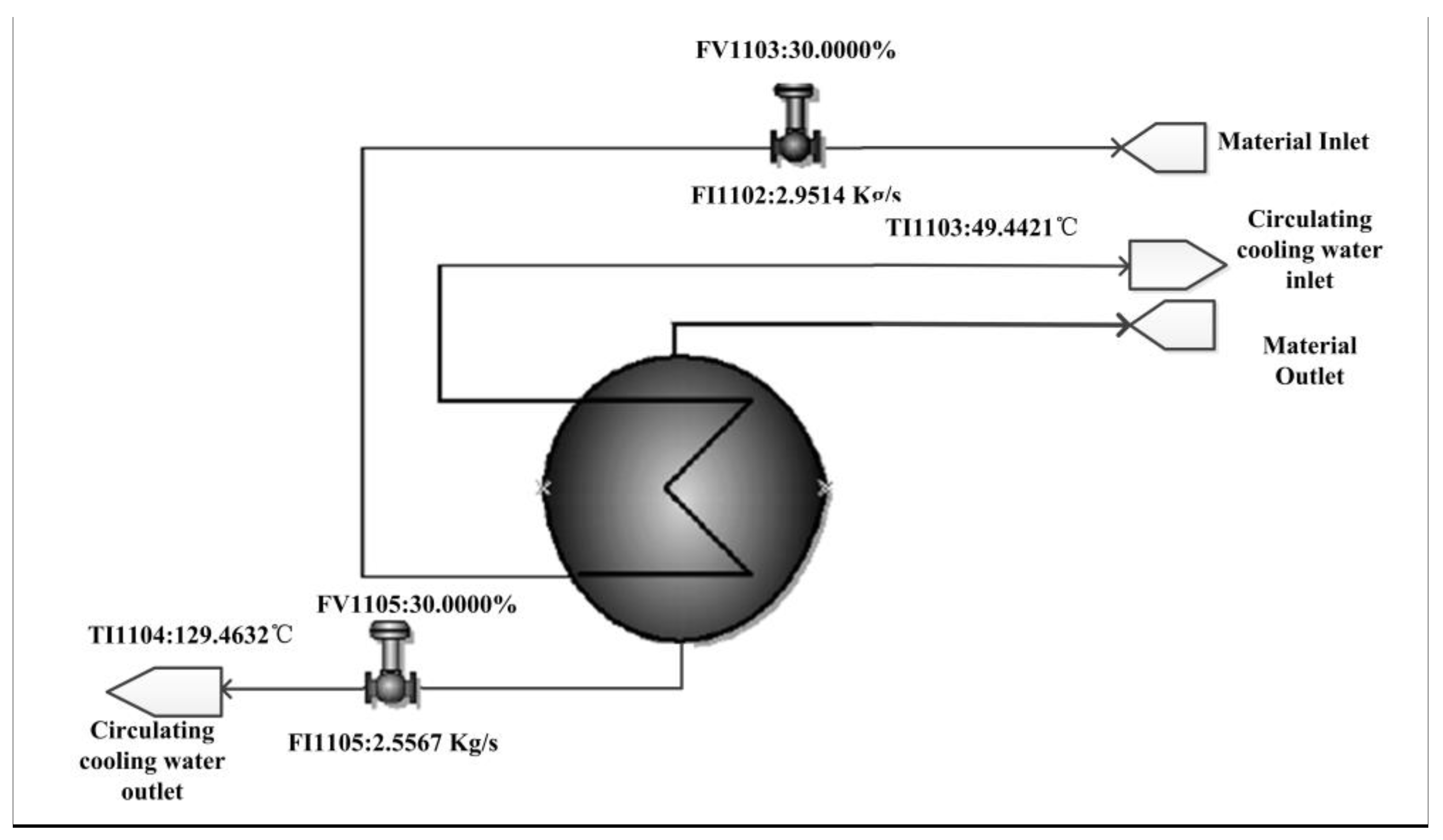
The heat exchange process is shown in Figure 9, FV1103 is the material inlet valve, its corresponding flow rate is FI1102, the temperature is TI1103, FV1105 is the utility water outlet valve, its corresponding flow rate is FI1105 and the corresponding temperature is TI1104.

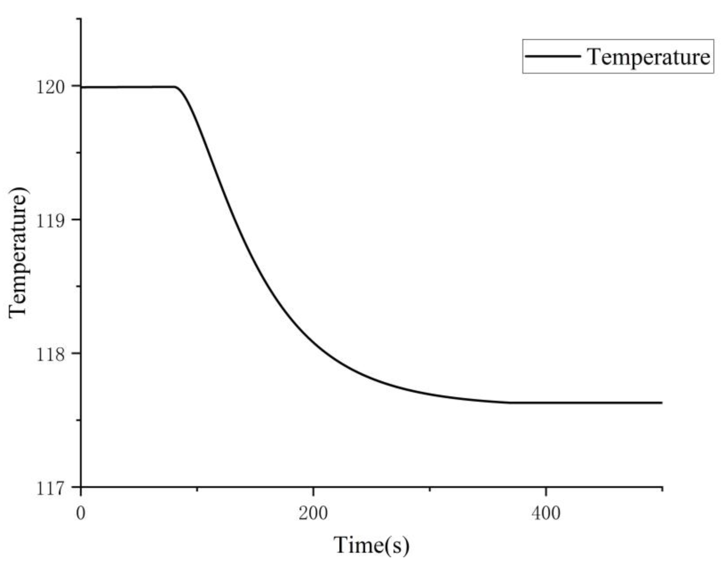
The FV1105 is manually given an opening of 35%, and since the temperature is a self-balancing system, it makes the TI1104 from the initial temperature reduced to a constant temperature, and an open-loop step curve of the heat exchanger outlet temperature is obtained, as shown in Figure 10.

With the open-loop response curve, the process transfer function can be obtained as in Equation (17).

$$G(s)=\frac{0.0274}{38731.2s^2+398.36s+1}{e}^{-30s}$$

(17)

4.2. Controller Design

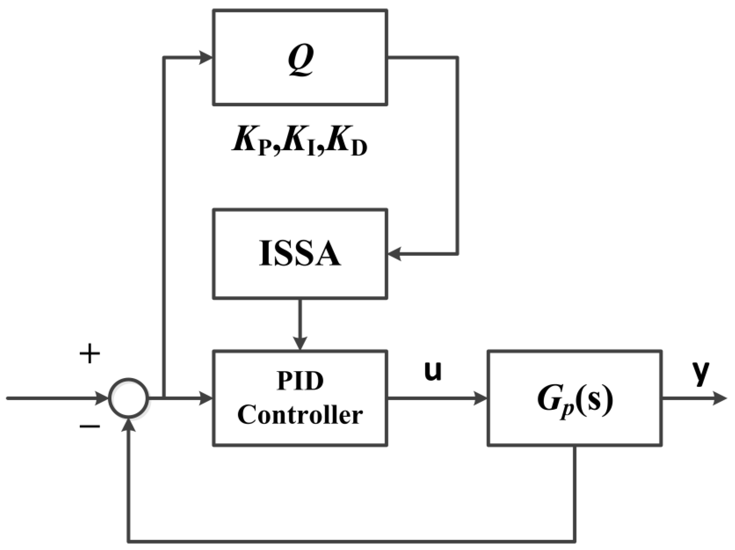
The quality of the parameters in the PID controller will greatly affect the quality of the controller. The purpose of this paper for the design of an optimized PID controller based on the improved sparrow search algorithm is to find an optimal set of parameters in the solution space $\left\{\left.K_{\mathrm{p}},K_{\mathrm{I}},K_{\mathrm{D}}\right\}\right.$, so that the system meets the control requirements and performs well.

In the design of the improved sparrow search algorithm PID controller, the objective function setting should be in accordance with the control system performance index, and satisfactory dynamic characteristics of the iterative process can be obtained, and the evaluation function $Q$ is set as shown in Equation (18).

$$Q={{\displaystyle \int }}_0^{\infty }\left(w_1|e(t)|+w_2{u}^2(t)\right)\mathrm{d}t$$

(18)

where $e(t)$ is the error of the output value with respect to the input value. $u(t)$ is a control value to avoid excessive control margins. $w_1$ is a weight value, taking the value [0, 1], in general $w_1=0.999$. $w_2$ is a weight value, taking the value [0, 1], in general $w_2=0.001$. Moreover, to prevent overshoot, a restriction is taken to prevent overshoot, i.e., when overshoot occurs, an overshoot term $w_3|e(t)|$ is introduced in the objective function $Q$ as shown in Equation (19).

$$Q={{\displaystyle \int }}_0^{\infty }\left(w_1|e(t)|+w_2{u}^2(t)+w_3|e(t)|\right)\mathrm{d}t$$

(19)

where $w_3$ is a Weights, set at $w_3=100$.

The improved sparrow search optimization algorithm is used to design the PID controller, setting the parameter range $K_{\mathrm{p}},K_{\mathrm{I}},K_{\mathrm{D}}\in [0,100000]$, and using Equation (19) as the fitness function, the objective of the optimization search is to find a set of PID values that minimize the error of $Q$ by rectifying the three parameters by ISSA.

The block diagram of the PID controller design based on the ISSA algorithm is shown in Figure 11, where $G_p(s)$ is a controlled system.

4.3. System Simulation and Results Analysis

4.3.1. Build Simulation Platform and Preliminary Performances Comparison

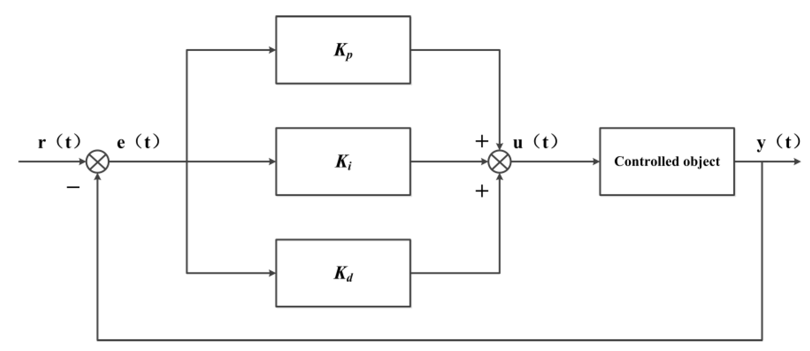
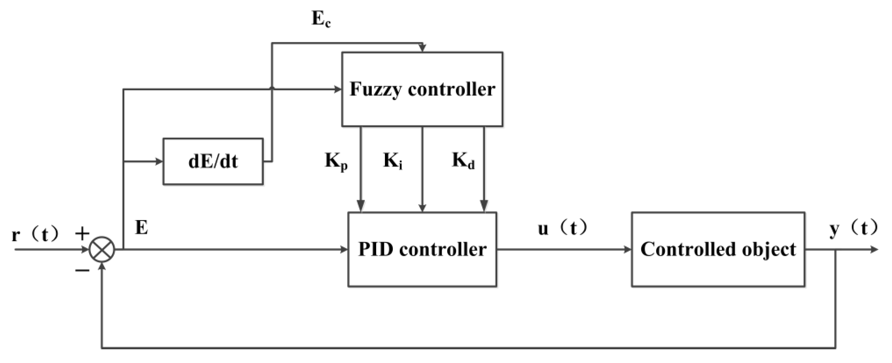
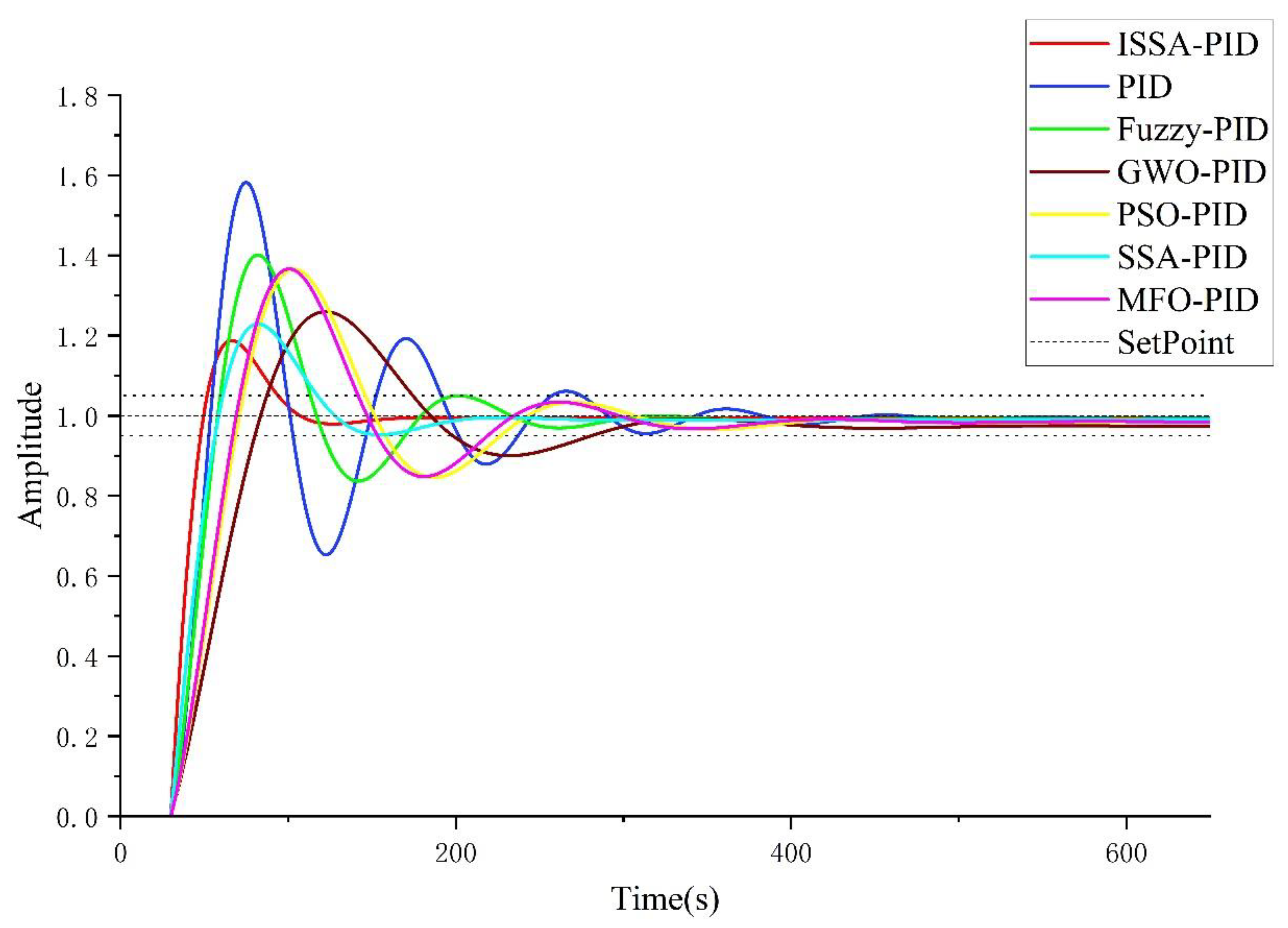
In the Simulink module of MATLAB, the traditional PID controller, fuzzy PID controller, PSO-PID controller, GWO-PID controller, MFO-PID controller, SSA-controller and ISSA-PID controller are built to compare the control effect on the unit step, the transfer function is Equation (17), the PID control block diagram is shown in Figure 12, the fuzzy PID control block diagram is shown in Figure 13, and the PID parameters of the seven controllers are shown in

Table 7. PID parameters.

Algorithm	Parameters
	KP	KI	KD
PID	6268.17706	0.02636	17,635.79
Fuzzy-PID	4224.04676	0.00533	31,417.79
ISSA-PID	6376.42771	0.00236	95,854.56
PSO-PID	2191.85053	0.00643	20,052.97
GWO-PID	1349.69954	0.00666	20,589.11
SSA-PID	3573.95374	0.00578	58,089.41
MFO-PID	2362.61431	0.00637	21,615.32

. The control effect comparison graph is shown is Figure 14.

Analyzing the data in Figure 14, the performance metrics of the various algorithm curves were obtained as shown in

Table 8. Performance index.

Algorithm	Performance Index
	Maximum Overshoot (%)	Peak Time (s)	Stable Time (s)	Steady-State Error (%)
PID	58.2	17.1	290.57	98.9
Fuzzy-PID	40.1	19.8	209.16	99.1
ISSA-PID	18.7	14.6	92.8	99.4
PSO-PID	36.5	32.8	228.96	98.2
GWO-PID	25.9	34.7	284.88	97.3
SSA-PID	22.8	35.8	117.80	98.9
MFO-PID	36.6	29.2	219.20	98.3

.

Setting the error band within 5%, as shown in Figure 14, ISSA-PID reduces overshoot by 9.5%, 21.4%, 17.8%, 7.2%, 4.1% and 17.9% compared to PID, Fuzzy-PID, PSO-PID, GWO-PID, SSA-PID and MFO-PID, respectively. The rise time is reduced by 2.5 s, 5.2 s, 18.2 s, 20.1 s, 21.2 s and 14.6 s; steady-state values are reduced by 197.77 s, 116.26 s, 136.16 s, 192.08 s, 25 s, 126.4 s. Steady-state values are all stable around 1.0, and ISSA-PID is 99.4, which is the lowest error compared to other controllers. Therefore, ISSA is optimal in all aspects of performance indexes.

In practical application environments, different perturbations are often encountered, and the cause of the perturbations may be caused by human control requirements or may be uncertain. Therefore, the algorithm is tested separately for the lift-load and perturbation tests as a way to verify the robustness of the algorithm.

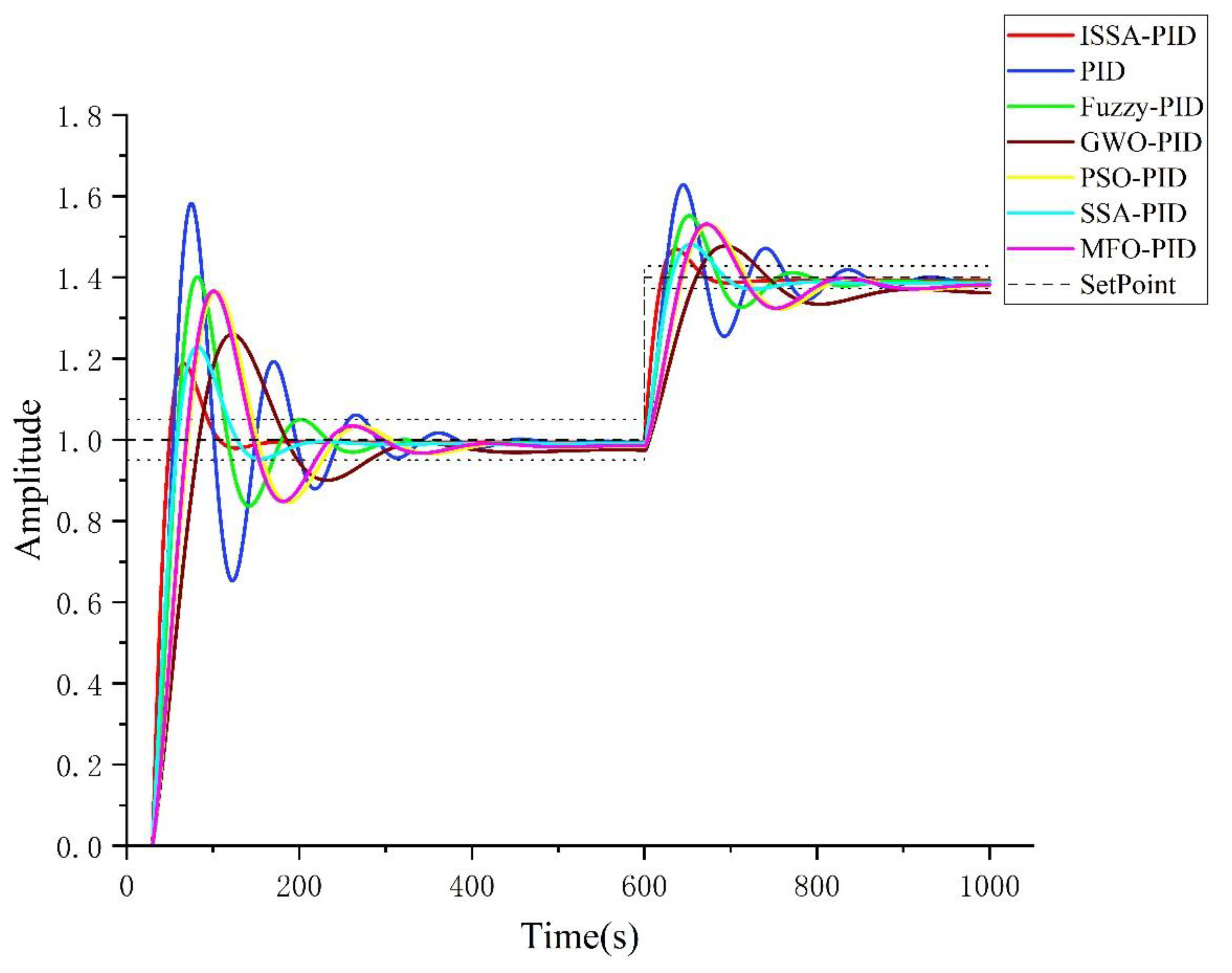
4.3.2. Liter Load Test

After the response curve is stabilized, the set value of the step response is increased from 1 to 1.4 at 600 s. The response curve of the control system is shown in Figure 15.

Reducing the error bar from 5% to 2% after ramping up the load, the performance indexes were obtained from the analysis of Figure 15 as shown in

Table 9. Performance index.

Algorithm	Performance Index
	Maximum Overshoot (%)	Peak Time (s)	Stable Time (s)	Steady-State Error (%)
PID	15.7	18.2	285.4	99.2
Fuzzy-PID	10.8	18.2	137.4	99.2
ISSA-PID	4.8	17.5	57.7	99.4
PSO-PID	9.2	30.6	362.9	98.5
GWO-PID	5.5	43.9	-	97.3
SSA-PID	5.9	21.3	144.5	98.9
MFO-PID	9.4	29.9	340	98.7

.

As shown in Figure 15, the steady-state value of ISSA-PID is improved by 0.2%, 0.2%, 0.9%, 2.1%, 0.5% and 0.7% compared with PID, Fuzzy-PID, PSO-PID, GWO-PID, SSA-PID and MFO-PID after increasing the load for 600 s, except for GWO-PID, which is finally stabilized within 2% error bars, In terms of transient performance, ISSA-PID overshoot improved by 10.9%, 6.0%, 4.4%, 0.7%, 1.1% and 4.6% compared with PID, Fuzzy-PID, PSO-PID, GWO-PID, SSA-PID, and MFO-PID, and the rise time decreased by 0.7 s, 0.7 s, 13.1 s and 26.6% compared with PID, Fuzzy-PID, PSO-PID, GWO-PID, SSA-PID, and MFO-PID s, 13.1 s, 26.4 s, 3.8 s and 12.4 s, and the adjustment time was reduced by 227.7 s, 79.7 s, 305.2 s, 86.8 s and 282.3 s compared to PID, Fuzzy-PID, PSO-PID, SSA-PID and MFO-PID, and the transient response speed was better than other algorithms. This shows the superiority of ISSA-PID in terms of control accuracy and response speed in the lift-load test.

4.3.3. Perturbation Test

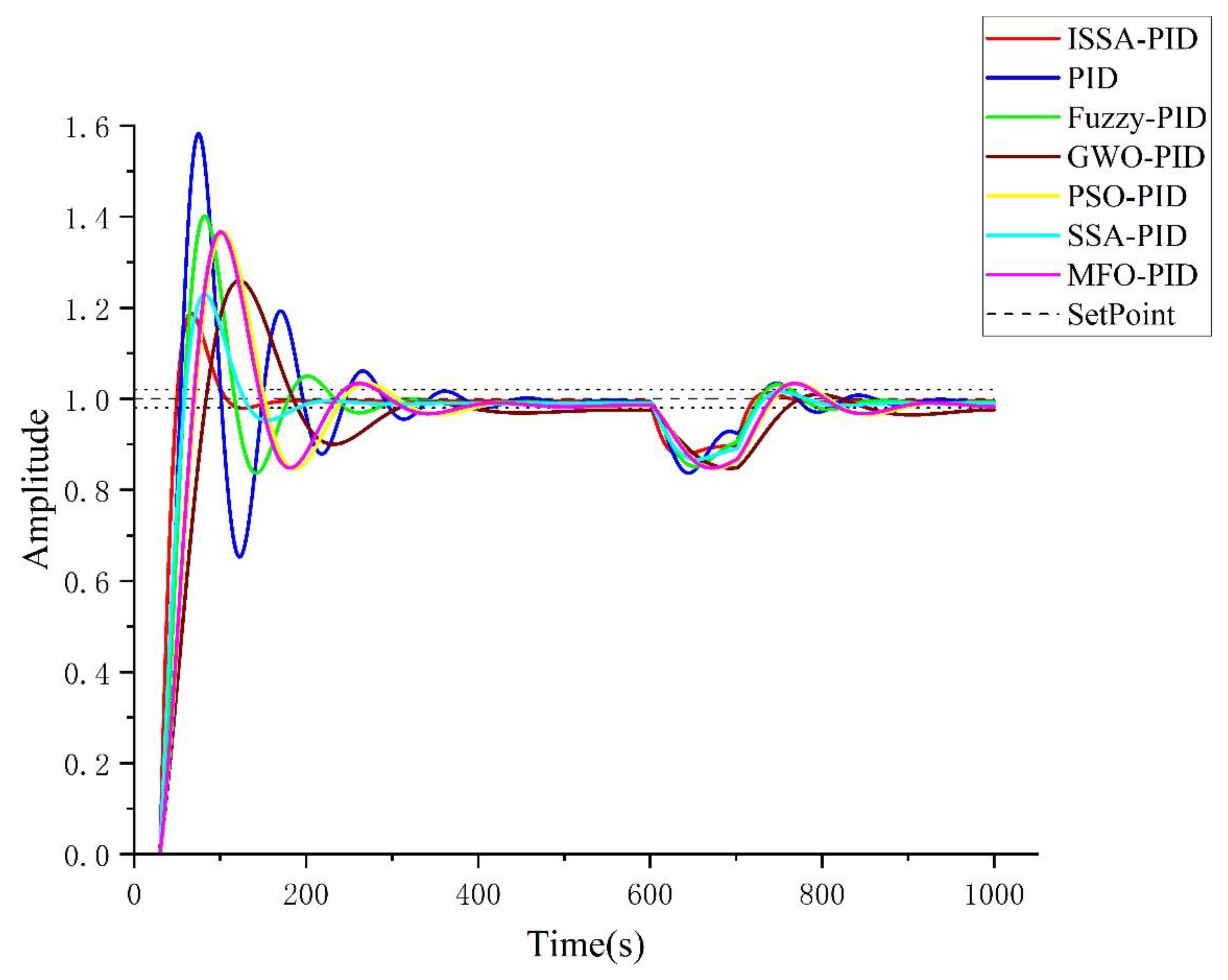
Again, a perturbation is applied to the system at 600 s to test the immunity of the algorithm to interference. The response curves are shown in Figure 16.

Analyzing Figure 16, compare the time for various controllers to recover to within 2% error bars after being disturbed by a 0.1 step signal at 600 s, as shown in

Table 10. Recovery time.

Algorithm	Recovery Time (s)
PID	210.9
Fuzzy-PID	223.1
ISSA-PID	114.2
PSO-PID	295.2
GWO-PID	-
SSA-PID	125.0
MFO-PID	284.2

.

The GWO-PID amplitude at 1000 s is still outside the 2% error bar, and the shortest time used by ISSA-PID is 114.2 s, which is 96.7 s faster than PID, 108.9 s faster than Fuzzy-PID, 181.0 s faster than PSO-PID, 170 s faster than MFO-PID, and the difference of recovery time is smaller compared with SSA-PID, but also faster 10.8 s, verifying that the ISSA-PID controller is more resistant to interference than other controllers.

5. Performance Analysis on Semi-Physical Platform Validation

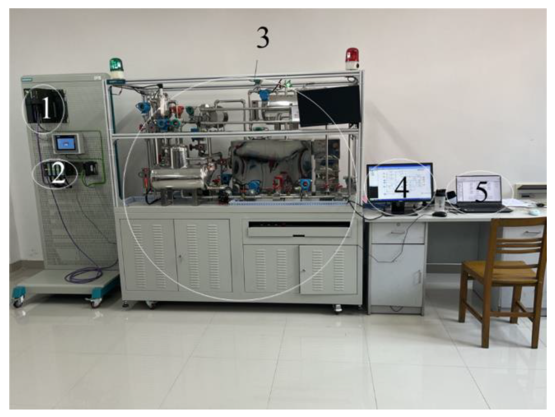
In order to test the actual control effect of the ISSA-PID controller, establish the experimental platform of continuously stirred tank reactor temperature control, through the upper computer SIMATIC PCS7 [28] software to write improved sparrow optimized PID controller algorithm, build OS (Operators Station) and AS (Automation Station) in the upper computer, regulate SMPT-1000 semi-physical platform through Profibus-DP bus for the experiment, the connect MATLAB and PCS7 communication through OPC (OLE for Process Control) technology. The final date curve is displayed on the IPC monitor. The test platform device is shown in Figure 17.

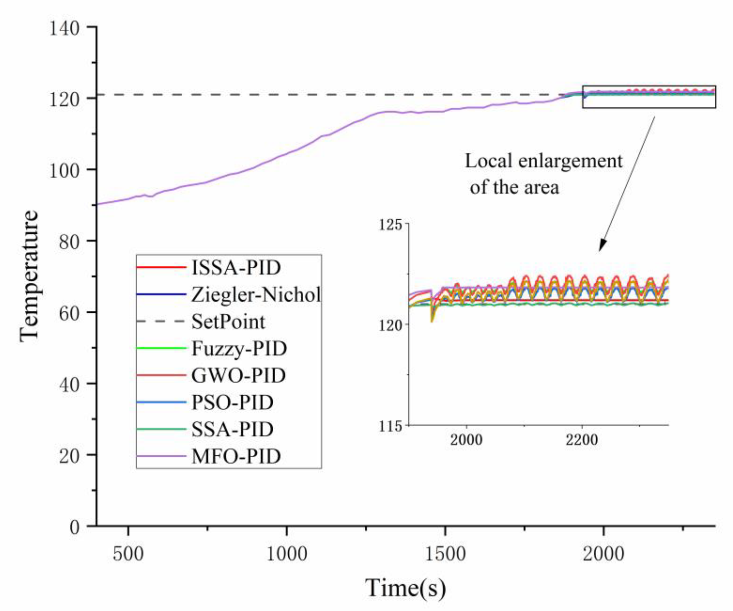
The temperature expectation was set at 121 °C, and the reactor temperature was controlled by controlling the opening of the upper water valve of the circulating cooling water through various optimization techniques, respectively, and the reactor temperature curve was obtained as shown in Figure 18.

Analyzing Figure 18, the performance indexes of various optimization techniques were obtained as shown in

Table 11. Performance index.

Algorithm	Performance Index
	Maximum Overshoot (%)	Peak Time (s)	Stable Time (s)	Steady-State Error (°C)
Z-N	0.24	24.1	165.1	0.4356
Fuzzy-PID	0.21	24.8	189.9	0.7678
ISSA-PID	0.10	21.0	68.2	0.1987
PSO-PID	0.14	20.0	172.3	0.3149
GWO-PID	0.31	21.6	160.1	0.7621
SSA-PID	0.12	21.0	70.2	−0.2587
MFO-PID	0.10	22.5	77.3	0.8362

. Since it is most important to keep the temperature stable near the working point among the working requirements of the reactor, the comparison of the steady-state error was focused on. The steady-state error of the curve with equal amplitude oscillation was taken as the middle value.

It can be seen from Figure 18 that the reactor changed the controller from manual to automatic at 1900 s, and various controllers started to control the opening size of valve FV1201 to regulate the circulating cooling water flow to control the temperature, and the seven algorithms could be stabilized around the set value after casting automatic, but only ISSA-PID and MFO-PID did not have equal amplitude oscillation, and the overshoot of both was 0.10%, which is 0.14%, 0.11%, 0.04%, 0.21% and 0.02% higher than Z-N, Fuzzy-PID, PSO-PID, GWO-PID and SSA-PID. In terms of rise time, PSO-PID has the best performance, only 20.0 s, which is actually 21.0 s of ISSA-PID and SSA-PID. ISSA-PID is slightly worse than PSO-PID; in terms of steady-state time, ISSA-PID is the best, shorter than Z-N, Fuzzy-PID, PSO-PID, GWO-PID, SSA-PID and MFO-PID by 96.9 s, 121.7 s, 104.1 s, 91.9 s, 2 s and 9.1 s. Finally, the most important steady-state error indicator, which is related to the quality of the final product of the reactor, because the closer the steady-state value is to the working point, the higher the conversion of the reaction product is. ISSA-PID is 0.1987, which is 0.2369 °C, 0.5691°C, 0.1162 °C, 0.5634 °C, 0.060 °C and 0.6375 °C lower than Z-N, Fuzzy-PID, PSO-PID, GWO-PID, SSA-PID and MFO-PID, respectively, the ISSA-PID controller has the best performance and meets the control requirements of reactor temperature.

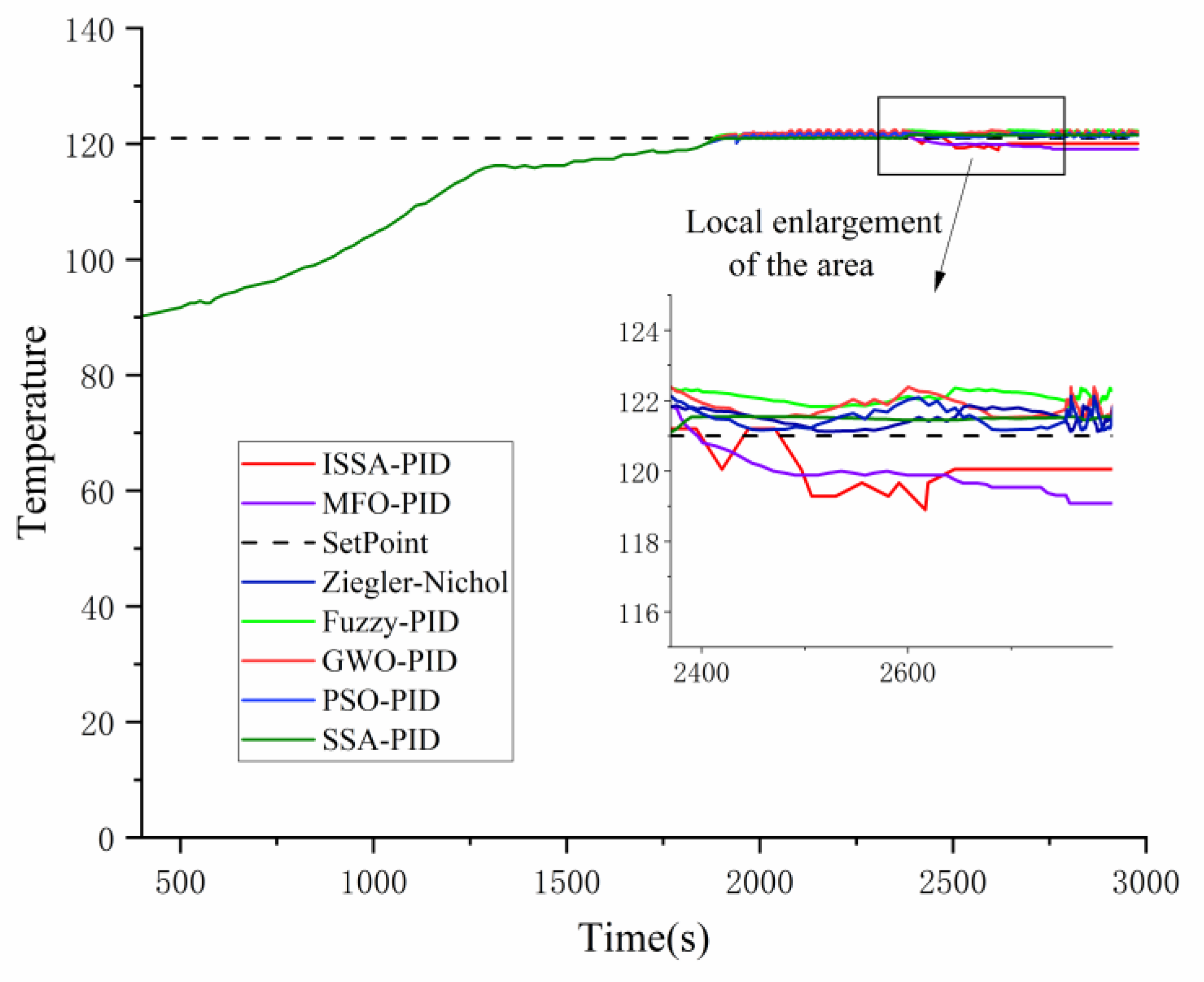
In practical application environments, different perturbations are often encountered, and the cause of the perturbations may be caused by human control requirements or may be uncertain. Therefore, a perturbation test is performed on the algorithm as a way to verify whether the robustness of the algorithm meets the requirements. The perturbation test plots for all algorithms are given, as shown in Figure 19.

Analyzing Figure 19, the valve openings controlled by both controllers were given a 2% perturbation at 2390 s to disturb the regulation of the reactor temperature, comparing the time required for both to return to the steady-state value and the final steady-state error, as shown in

Table 12. Performance index.

Algorithm	Recovery Time (s)	Steady-State Error (°C)
Z-N	392.9	2.128
Fuzzy-PID	397.0	1.360
ISSA-PID	250.3	0.952
PSO-PID	423.0	1.032
GWO-PID	411.2	1.385
SSA-PID	427.6	0.803
MFO-PID	381.7	1.923

.

Through the disturbance test, the ISSA-PID controller recovered the steady-state after 250.3 s, which is 142.6 s, 146.7 s, 172.7 s, 160.9 s, 177.3 s, 131.4 s less than Z-N, Fuzzy-PID, PSO-PID, GWO-PID, SSA-PID and MFO-PID, respectively, which greatly reduces the recovery time. The steady-state value of the ISSA-PID controller is 120.048 °C and the error between the set value and 121 °C is only 0.952 °C, which is 1.176 °C, 0.408 °C, 0.08 °C, 0.433 °C and 0.971 °C smaller than the steady-state errors of Z-N, Fuzzy-PID, PSO-PID, GWO-PID and MFO-PID, respectively. Therefore, the ISSA-PID controller has excellent performance in terms of speed and accuracy in the face of disturbances and can meet the requirements of continuous reactor temperature control with certain robustness.

6. Conclusions and Future Perceptive

In this work, a reactor temperature control method based on an improved sparrow algorithm to optimize PID parameters is proposed. Firstly, the traditional sparrow algorithm is improved by introducing tent chaos mapping in the initialization process of algorithm iteration to improve the initial solution quality. Meanwhile, the golden sine is introduced to improve the discoverer position update formula, which reduces the solution space and further improves the optimal search effect of ISSA, and the Gauss–Cauchy mutation strategy iteration is introduced to improve the local optimization capability. By comparing with four existing classical algorithms, namely GWO, PSO, MFO and SSA, the results show that ISSA has a stronger and more robust search capability, and the convergence speed meets real-time requirements.

After establishing the heat exchanger model and identifying its parameters, the ISSA-PID controller is designed, and the control curves of the ISSA-PID controller are compared with those of classical PID control and fuzzy PID control under different control requirements through experimental simulation, and the conclusion that the overall control performance of ISSA-PID controller is better is drawn.

Finally, by establishing a semi-physical experimental platform based on PCS7 and SMPT-1000, it is verified that the ISSA-PID controller designed in this paper meets the system response requirements, has superior performance in terms of adjustment time and steady-state error and has certain robustness.

The subsequent research extends the application area of the algorithm in this paper to apply the ISSA-PID controller to more complex systems, such as the internal circulation reactor used for integrated CO2 capture and power generation.

References

- Yang, C.-F.; Wang, C.-C.; Tseng, C.-H. Methylamine removal using mixed bacterial strains in a continuous stirred tank reactor (CSTR) system. Int. Biodeterior. Biodegrad. 2013, 85, 583–586. [Google Scholar] [CrossRef]
- Gargouri, B.; Aloui, F.; Sayadi, S. Reduction of petroleum hydrocarbons content from an engine oil refinery wastewater using a continuous stirred tank reactor monitored by spectrometry tools. J. Chem. Technol. Biotechnol. 2012, 87, 238–243. [Google Scholar] [CrossRef]
- Vlassis, T.; Stamatelatou, K.; Antonopoulou, G. Methane production via anaerobic digestion of glycerol: A comparison of conventional (CSTR) and high-rate (PABR) digesters. J. Chem. Technol. Biotechnol. 2013, 88, 2000–2006. [Google Scholar] [CrossRef]
- Tobita, H. Free-Radical Polymerization with Long-Chain Branching and Scission in a Continuous Stirred-Tank Reactor. Macromolecular React. Eng. 2013, 7, 181–192. [Google Scholar] [CrossRef]
- Esfandyari, M.; Fanaei, M.A.; Zohreie, H. Adaptive fuzzy tuning of PID controllers. Neural Comput. Appl. 2013, 23, 19–28. [Google Scholar] [CrossRef]
- Atif, S.M.; Nishat, A.M.; Laskar, S.H. Control of nonlinear jacketed continuous stirred tank reactor using different control structures. J. Process Control. 2021, 108, 112–124. [Google Scholar]
- Djarum, D.H.; Ahmad, Z. Designing real time model mobile monitoring system for model predictive control in a nonlinear continuous stirred tank reactor. Asia-Pac. J. Chem. Eng. 2020, 15, e2430. [Google Scholar] [CrossRef]
- Alshammari, O.; Mahyuddin, M.N.; Jerbi, H. An Advanced PID Based Control Technique With Adaptive Parameter Scheduling for A Nonlinear CSTR Plant. IEEE Access 2019, 7, 158085–158094. [Google Scholar] [CrossRef]
- Sudhanan, R.M.; Poongodi, D.P. Comparative Analysis of Various Control Strategies for a Nonlinear CSTR System. Int. J. Nonlinear Sci. Numer. Simul. 2017, 18, 269–276. [Google Scholar] [CrossRef]
- Chopra, V.; Singla, S.K.; Dewan, L. Comparative Analysis of Tuning a PID Controller using Intelligent Methods. Acta Polytech. Hung. 2014, 11, 235–249. [Google Scholar]
- Mukherjee, D.; Raja, G.L.; Kundu, P.; Ghosh, A. Improved fractional augmented control strategies for continuously stirred tank reactors. Asian J. Control 2022, 10, 1002. [Google Scholar] [CrossRef]
- Stavrov, D.; Nadzinski, G.; Deskovski, S.; Stankovski, M. Quadratic Model-Based Dynamically Updated PID Control of CSTR System with Varying Parameters. Algorithms 2021, 14, 31. [Google Scholar] [CrossRef]
- Xue, J.; Shen, B. A novel swarm intelligence optimization approach: Sparrow search algorithm. Syst. Sci. Control. Eng. 2020, 8, 22–34. [Google Scholar] [CrossRef]
- Li, Q.; Shi, Y.; Lin, R.; Qiao, W.; Ba, W. A novel oil pipeline leakage detection method based on the sparrow search algorithm and CNN. Measurement 2022, 204, 112122. [Google Scholar] [CrossRef]
- Xu, J.-H.; Xu, H.-Z.; Ding, Q.; Zhu, K.-Q.; Yang, Y.-R.; Wang, Y.-L.; Huang, T.-M.; Chen, X.; Wan, Z.-M.; Wang, X.-D. Sparrow search algorithm applied to temperature control in PEM fuel cell systems. Int. J. Hydrog. Energy 2022, 47, 39973–39986. [Google Scholar] [CrossRef]
- Duan, M.; Yang, Z.; Zhao, Y.; Fang, L.; Zuo, H.; Li, Z.; Wang, D. Wavefront shaping using improved sparrow search algorithm to control the scattering light field. Opt. Laser Technol. 2022, 156, 108529. [Google Scholar] [CrossRef]
- Sun, C.; Liu, P.; Guo, H.; Di, Y.; Xu, Q.; Hao, X. Control of Precalciner Temperature in the Cement Industry: A Novel Method of Hammerstein Model Predictive Control with ISSA. Processes 2023, 11, 214. [Google Scholar] [CrossRef]
- Zhang, H.; Yang, J.; Qin, T.; Fan, Y.; Li, Z.; Wei, W. A Multi-Strategy Improved Sparrow Search Algorithm for Solving the Node Localization Problem in Heterogeneous Wireless Sensor Networks. Appl. Sci. 2022, 12, 5080. [Google Scholar] [CrossRef]
- Zhu, Q.; Zhuang, M.; Liu, H.; Zhu, Y. Optimal Control of Chilled Water System Based on Improved Sparrow Search Algorithm. Buildings 2022, 12, 269. [Google Scholar] [CrossRef]
- Wang, Y.; Gao, S.; Yu, Y.; Wang, Z.; Cheng, J.; Yuki, T. A Gravitational Search Algorithm With Chaotic Neural Oscillators. IEEE Access 2020, 8, 25938–25948. [Google Scholar] [CrossRef]
- Tanyildizi, E.; Demir, G. Golden Sine Algorithm: A Novel Math-Inspired Algorithm. Adv. Electr. Comput. Eng. 2017, 17, 71–78. [Google Scholar] [CrossRef]
- Wang, W.C.; Xu, L.; Chau, K.W.; Xu, D.M. Yin-Yang firefly algorithm based on dimensionally Cauchy mutation. Expert Syst. Appl. 2020, 150, 113216. [Google Scholar] [CrossRef]
- Saeed, S.; Ong, H.C.; Sathasivam, S. Self-Adaptive Single Objective Hybrid Algorithm for Unconstrained and Constrained Test functions: An Application of Optimization Algorithm. Arab. J. Sci. Eng. 2019, 44, 3497–3513. [Google Scholar] [CrossRef]
- Kohli, M.; Arora, S. Chaotic grey wolf optimization algorithm for constrained optimization problems. J. Comput. Des. Eng. 2018, 5, 458–472. [Google Scholar] [CrossRef]
- Cruz, L.M.; Alvarez, D.L.; Al-Sumaiti, A.S.; Rivera, S. Load Curtailment Optimization Using the PSO Algorithm for Enhancing the Reliability of Distribution Networks. Energies 2020, 13, 3236. [Google Scholar] [CrossRef]
- Bingul, Z.; Karahan, O. Comparison of PID and FOPID controllers tuned by PSO and ABC algorithms for unstable and integrating systems with time delay. Optim. Control. Appl. Methods 2018, 39, 1431–1450. [Google Scholar] [CrossRef]
- Xu, Y.; Chen, H.; Luo, J.; Zhang, Q.; Jiao, S.; Zhang, X. Enhanced Moth-flame optimizer with mutation strategy for global optimization. Inf. Sci. 2019, 492, 181–203. [Google Scholar] [CrossRef]
- Kazemi, Z.; Safavi, A.A.; Pouresmaeeli, S.; Naseri, F. A practical framework for implementing multivariate monitoring techniques into distributed control system. Control. Eng. Pract. 2019, 82, 118–129. [Google Scholar] [CrossRef]
Figure 1.
Traditional SSA flow chart.
Figure 2.
Tent Chaos Sequence.
Figure 3.
ISSA flow chart.
Figure 4.
High-dimensional single-peak function convergence curve.
Figure 5.
High-dimensional multi-peak functions convergence curve.
Figure 6.
Fixed-dimensional multimodal function convergence curve.
Figure 7.
Complicated function convergence curve.
Figure 8.
Schematic diagram of heat exchanger structure.
Figure 9.
Process flow diagram of heat exchange process.
Figure 10.
Heat exchanger outlet temperature open loop step curve.
Figure 11.
Block diagram of optimized PID controller design based on improved sparrow algorithm.
Figure 12.
PID control block diagram.
Figure 13.
Fuzzy PID control block diagram.
Figure 14.
Control effect comparison curve.
Figure 15.
Lifting load response curve.
Figure 16.
Response curve of the applied disturbance.
Figure 17.
Experimental equipment and devices: 1. SIMATIC S7-400 PLC; 2. ET200M; 3. SMPT-1000 experiment platform; 4. Industrial control machine monitor; 5. Upper computer.
Figure 18.
Reactor temperature curve.
Figure 19.
Perturbation test curve graph.