
Quantitative Interpretation Model of Interwell Tracer for Fracture-Cavity Reservoir Based on Fracture-Cavity Configuration
1
School of Petroleum Engineering, Xi’an Shiyou University, Xi’an 710065, China
2
Engineering Research Center of Development and Management for Low to Extra-Low Permeability Oil & Gas Reservoirs in West China, Ministry of Education, Xi’an 710065, China
3
School of Energy Engineering, Longdong University, Qingyang 745000, China
4
Changqing Oilfield Company Oil Production Plant NO. 10, Petrochina, Qingyang 745100, China
5
Changqing Oilfield Company Oil Production Plant NO. 6, Petrochina, Yulin 710200, China
6
Northwest Oilfield Company, Sinopec, Luntai 841604, China
*
Author to whom correspondence should be addressed.
Processes 2023, 11(3), 964; https://doi.org/10.3390/pr11030964
Submission received: 8 February 2023
/
Revised: 7 March 2023
/
Accepted: 13 March 2023
/
Published: 21 March 2023
(This article belongs to the Special Issue Geological and Engineering Problems in the Development of Unconventional Oil and Gas Reservoirs)
Abstract
:The fracture-cavity combination structure between wells in fracture-cavity reservoirs is complex and changeable. Reliably identifying and quantitatively characterizing the fracture-cavity combination structure between wells has become an important prerequisite for flow channel adjustment in fracture-cavity reservoirs after water channeling and flooding. Aiming at the problems that it is difficult for the existing carving technology to characterize the flow characteristics of the injected fluid in the interwell fracture-cavity composite structure during the production process, and it is difficult for the existing interwell tracer proxy model to consider the specific fracture-cavity composite structure, this paper proposes a quantitative interpretation model for interwell tracers in fracture-cavity reservoirs with different architectures. Taking the Tahe fracture-cavity reservoir as the object, the matching relationship between the interwell fracture-cavity structure and the tracer curve was analyzed, and the tracer curve characteristics of five types of fracture-cavity structures were clarified. Considering the basic idea of tracing, a unified quantitative interpretation model of tracers under different fracture-cavity configurations based on branched flow channels and karst caves was deduced and established, and the input parameters required to apply the model, the parameters obtained directly by fitting, and further expandable calculated parameters were clarified. The interpretation model was used to fit, quantitatively interpret, and verify the reliability of the tracer curves of three wells in group TK411 of fracture-cavity unit S48 in the fourth area of Tahe Oilfield. The results show that the tracer curve fitting effect of each well was good, and the average relative error between the total flow rate explained by the tracer and the daily water production during the tracer monitoring period in the mine was only 3.02%, which effectively shows that the applicability and reliability of the quantitative interpretation model are established. The research results provide an effective way to apply tracer data in deep mining while improving the quantitative characterization ability of interwell tracer monitoring in fracture-cavity reservoirs.
1. Introduction
Worldwide, fracture-cavity carbonate reservoirs are rich in reserves and are among the most important oil and gas resources [1,2]. Fracture-cavity reservoirs are very heterogeneous; the reservoir space is mainly fractures, karst caves, pores, karst pipes, etc., and their horizontal and vertical connection modes are complex and diverse [1,2,3,4]. Primary oil recovery mainly relies on widely developed edge and bottom water energy, and methods such as water injection and gas injection are also adopted to enhance oil recovery [4,5]. Affected by the complex fracture-cavity combination structure of such reservoirs, water channeling and flooding are likely to occur during water and gas injection, and the development effect is greatly reduced [4,5,6,7]. Therefore, the reliable identification and quantitative characterization of the fracture-cavity combination structure between wells has become an important prerequisite for flow channel adjustment after water channeling and flooding in fracture-cavity reservoirs [4,5,6,7,8,9,10].
At present, the sculpting of fracture-cavity reservoirs mainly relies on factors such as seismic, core, conventional/imaging logging, drilling and logging, and well testing. It is difficult to reflect the flow characteristics of the injected fluid in the fracture-cavity combination structure between wells, which is very important for the water and gas injection development of this type of reservoir, during the production process [11,12,13,14,15,16,17]. An interwell tracer can follow, track, and mark the flow track of the injected fluid and can visually indicate the interwell connectivity status. Other monitoring methods are not comparable to interwell tracers for monitoring interwell fluid flow. Its application in water and gas injection in fracture-cavity reservoirs is becoming more extensive [18,19,20,21,22].
At present, interwell tracer interpretation for fracture-cavity reservoirs is mostly limited to using the injected water distribution coefficient, water injection advance rate, main water injection direction of the well group, and contribution of liquid production and swept volume to determine the interwell connectivity in a general way [18,19,20,21,22,23,24]. In terms of quantitatively characterizing fracture-cavity parameters, the complex combined structure is simplified into a series of flow tube bundles, and an equivalent proxy model of an interwell tracer in a fracture-cavity reservoir is established by using the convection–diffusion theory [25,26,27,28,29]. Although this model does not consider the specific fracture-cavity combination structure between wells, it is useful for the quantitative interpretation of interwell tracers in fracture-cavity reservoirs [25,26,27,28,29].
With the continuous development of interwell tracer interpretation technology, the morphological characteristics of the tracer concentration curve can basically determine the interwell fracture-cavity combination structure; for example, the tracer concentration curve of a single fracture between wells is unimodal with two basically symmetrical wings, while a single karst cave between wells has a unimodal curve with an obvious tailing phenomenon, with a steep ascending branch and slow descending branch. These findings have been verified by various experiments [30,31,32,33,34,35], which lays a reliable foundation for the establishment of quantitative interpretation models of interwell tracers in fracture-cavity reservoirs with different architectures.
Therefore, this paper takes the fracture-cavity reservoir in Tahe Oilfield as the object and analyzes the matching relationship between the fracture-cavity configuration and the tracer curve in the reservoir. We identify the tracer curve characteristics of five types of fracture-cavity structures: interwell pipes/fractures, interwell karst caves, and interwell pipes/fractures in parallel. Based on this, different fracture-cavity architectures are unified, a mathematical model of tracer migration between wells in fracture-cavity reservoirs is deduced and established, and the corresponding analytical solutions are obtained. Using this model, tracer curve fitting and quantitative interpretation are carried out for the field example of the Tahe fracture-cave reservoir, and the interpretation results are verified by the production performance data. The research results provide an effective way to apply tracer data in deep mining and fractured-cavity reservoirs and improve the quantitative characterization ability of interwell tracer monitoring.
2. Matching Relationship between Fracture-Cavity Configuration and Tracer Curve
After a fracture-cavity reservoir has experienced multiple tectonic movements and suffered severe weathering, denudation, and leaching, the shape of the reservoir, which is composed of dissolved caves, fractures, and dissolved pores, will become disordered and randomly distributed, and the interwell-connected structures will be difficult to identify [21,26,27]. However, the distribution characteristics of fracture-cavity reservoirs and the principle of well distribution determine that the interwell connectivity mode is mainly a single channel. Taking the Ordovician fracture-cavity carbonate reservoir in Tahe Oilfield as an example, among the tracer response wells (BY series of tracers), 73.5% of the tracer curves reflect a single channel, and only 16.5% reflect multiple channels [21,26,27]. The tracer monitoring data between the wells in Tahe Oilfield were collected and sorted, then combined with drilling, logging, core, testing, and production performance data, with the previous data used for reference. Meanwhile, referring to previous physical model experiments with tracer production [21,26,27,34,35], the interwell channels were divided into single-channel and multi-channel types, and the matching relationship between interwell fracture-cavity configuration and tracer curve could be determined.
2.1. Single-Channel Interwell
2.1.1. Interwell Pipe/Fracture Structure and Its Tracer Curve Characteristics
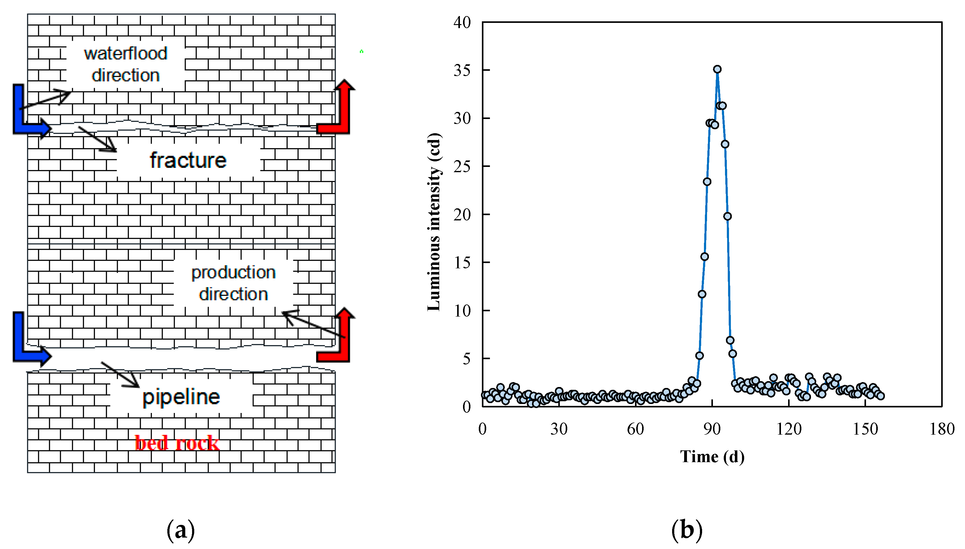
In the interwell pipe/fracture structure, the tracer flows through a single channel with no forks, small volume, and a fast flow rate. The tracer curve generally shows a regular peak shape with two basically symmetrical wings. The response time bandwidth is narrow (Figure 1).
2.1.2. Interwell Karst Cave Structure and Its Tracer Curve Characteristics
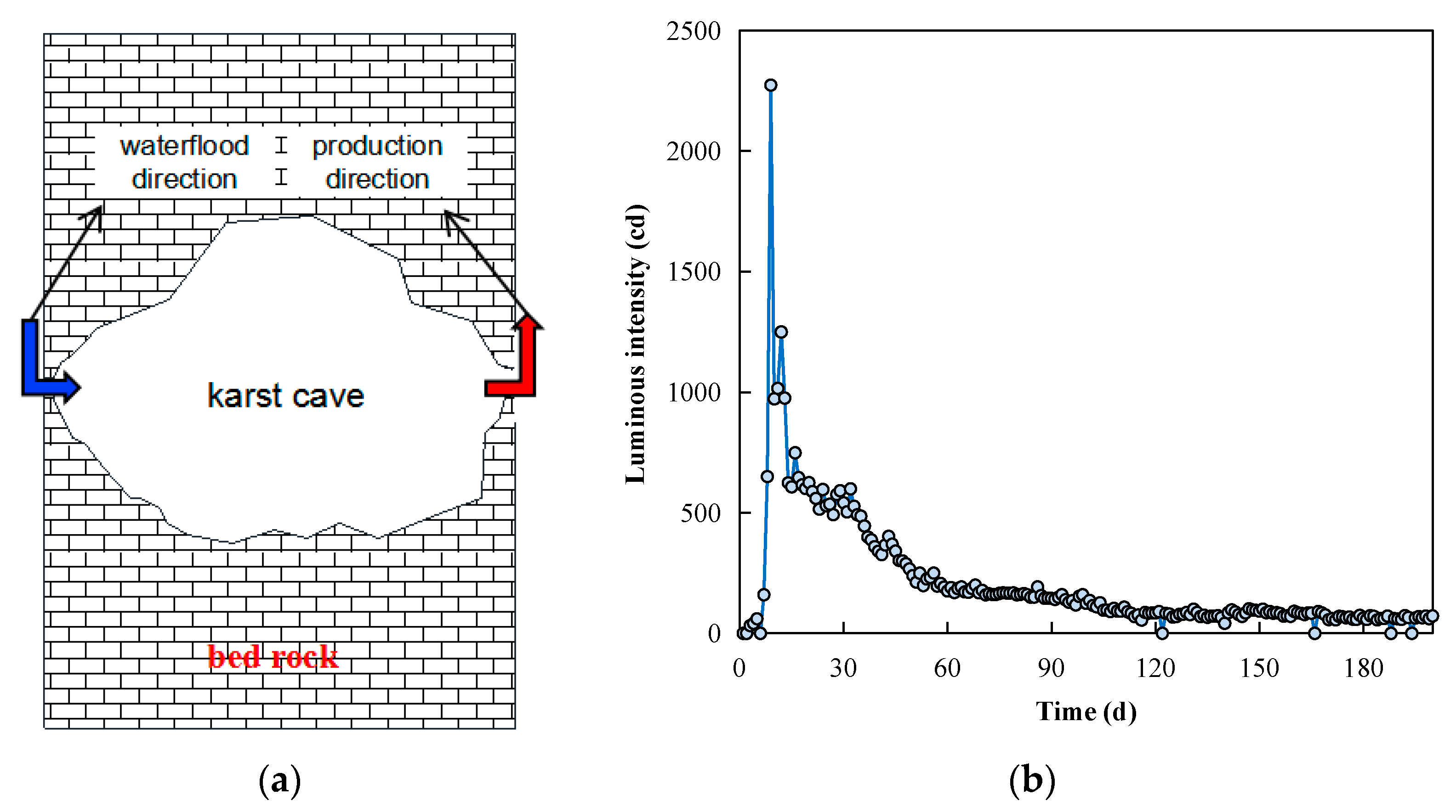
In the interwell karst cave structure, due to the huge interconnected volume between wells, the slow migration speed of the tracer, and the dilution and diffusion of the tracer during the migration process, the migration time is greatly prolonged. Therefore, the tracer output curve of this type of structure generally shows the characteristics of a steep ascending wing and a slow descending wing; the effective response time bandwidth of the tracer is long, and the descending wing shows an obvious trailing phenomenon (Figure 2).
2.2. Multi-Channel Interwell
2.2.1. Interwell Parallel Pipe/Fracture Structure and Its Tracer Curve Characteristics
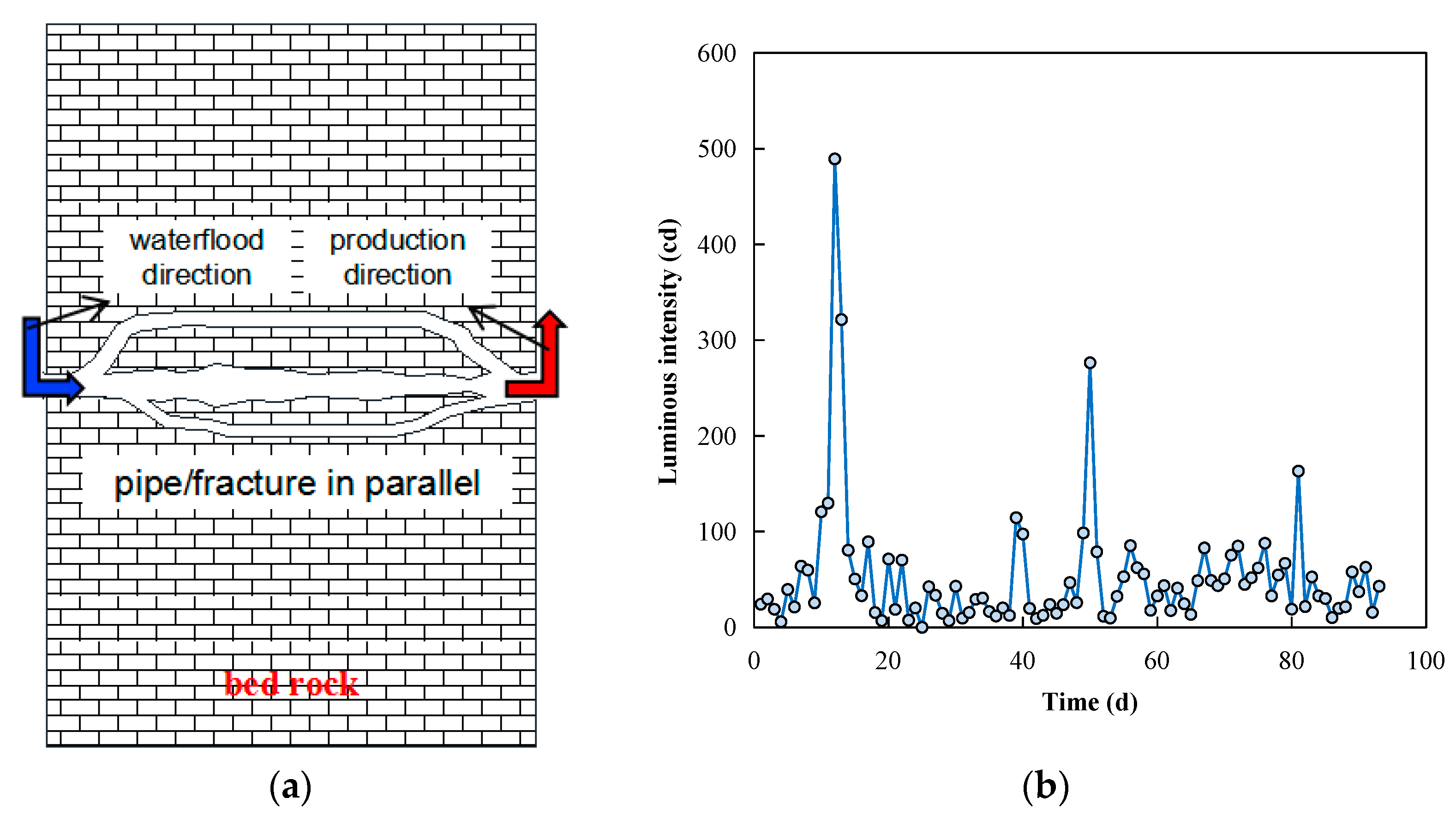
Each peak of the tracer curve in the interwell parallel pipe/fracture structure generally shows a sharp knife-like characteristic with two basically symmetrical wings. If the flow difference of the branch channels is large, the tracers of each branch are produced in sequence, and their production times are independent of each other. The curve shows the form of multiple independent peaks, and the sharp narrow peak of the main channel usually appears earlier, with the number of peaks reflecting the number of parallel channels (Figure 3). If the flow difference of the branch channels is small, the tracer production time of the two branches will overlap. The curve shows a continuous multi-peak shape, and the descending wing has a slight tail, but the continuous peak duration is short.
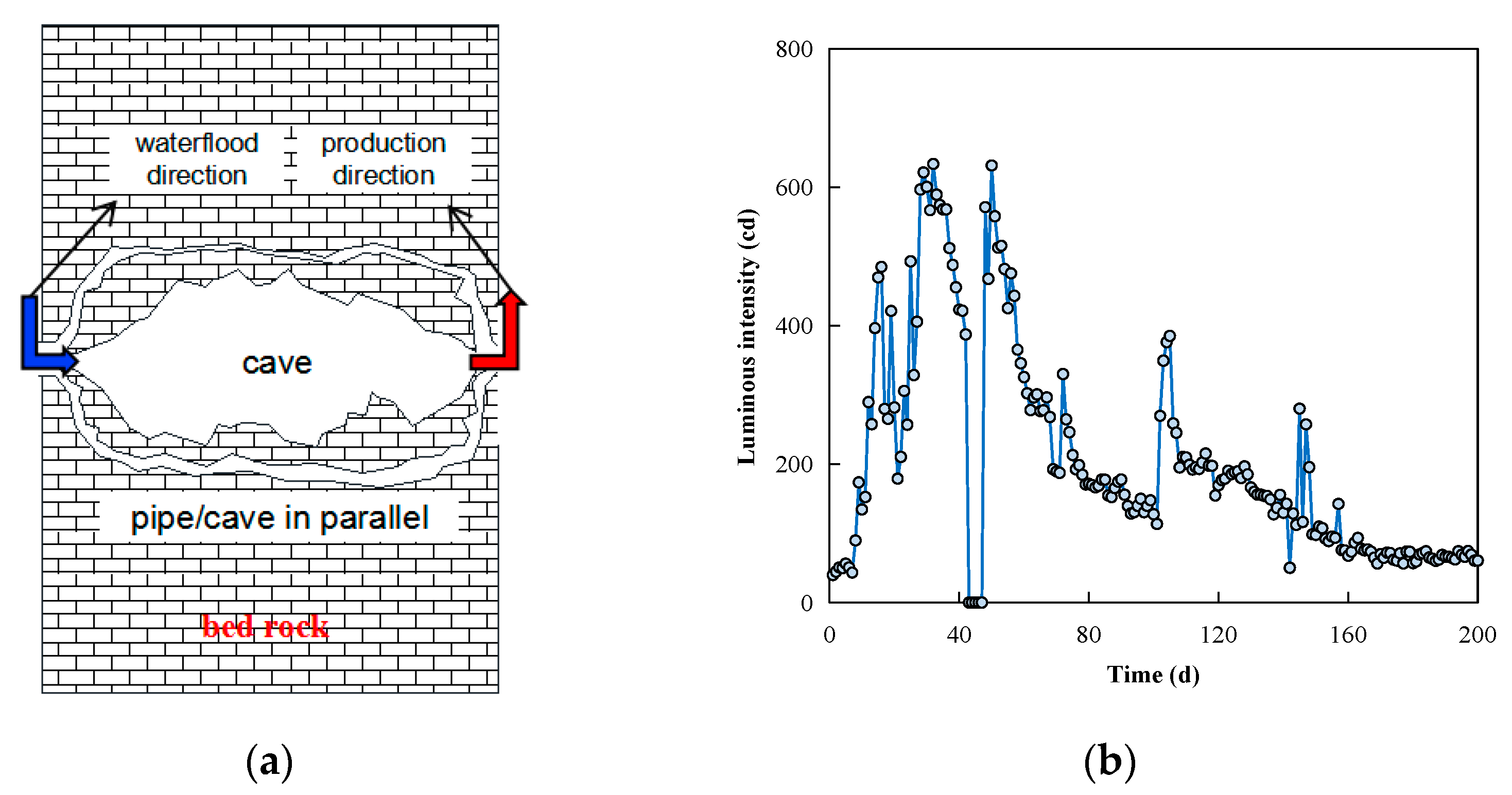
2.2.2. Interwell Parallel Karst Cave Structure and Its Tracer Curve Characteristics
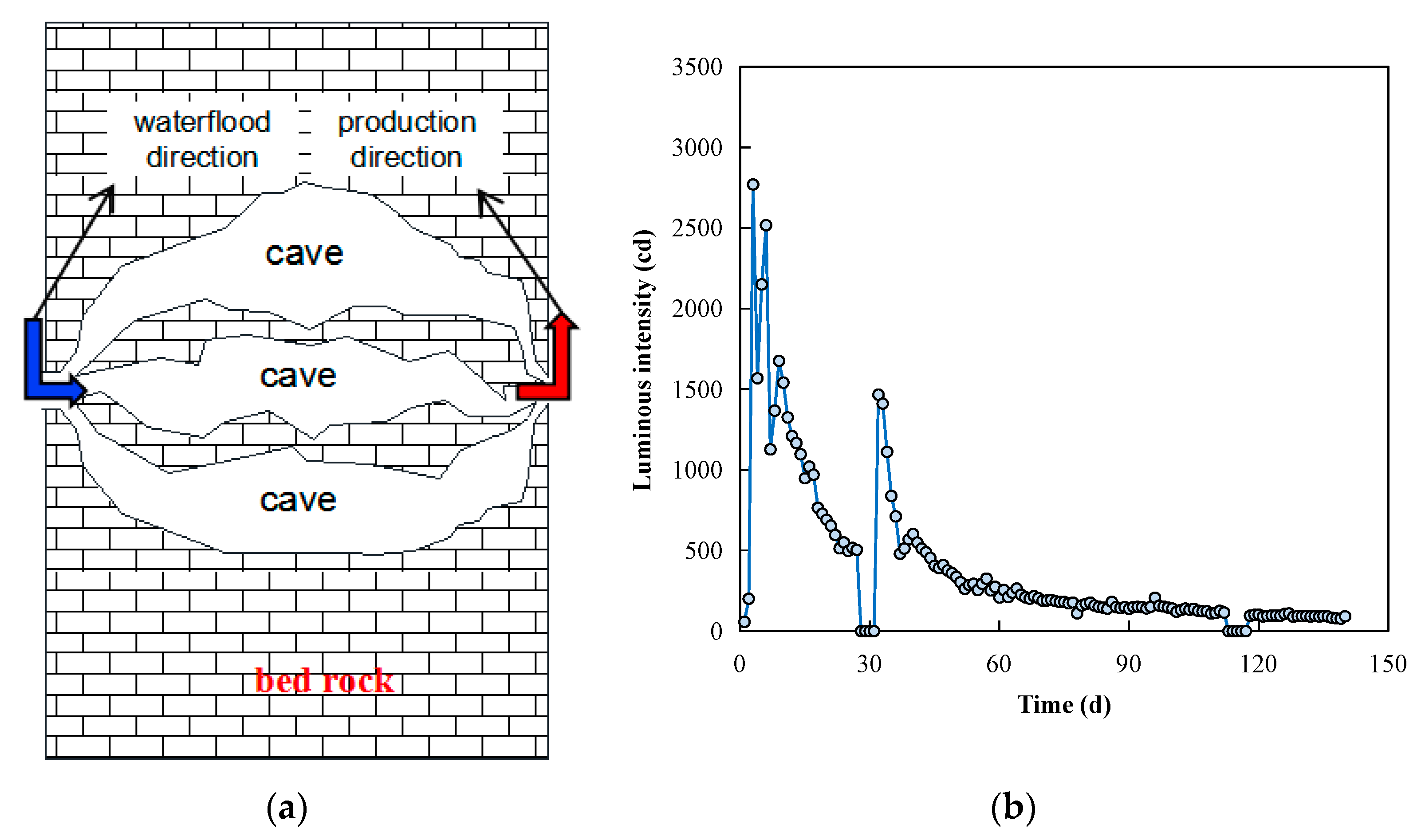
Each peak of the tracer curve of the parallel structure of karst caves between wells generally shows the characteristics of a sharp ascending wing and a slow descending wing. If the flow difference of the branch channels is large, the form of the curve is multiple independent peaks, and the peak of the main channel usually appears earlier, with the number of peaks reflecting the number of parallel channels and the severity of tailing reflecting the size of the cave (Figure 4). If the flow difference of the branch channels is small, the tracer output time of the two branches will partially overlap. The curve shows a continuous multi-peak shape, and the trailing time of the descending wing is long.
2.2.3. Interwell Parallel Pipe/Karst Cave Structure and Its Tracer Curve Characteristics
The tracer curve of the interwell parallel pipe/karst cave structure generally has the characteristics of sharp and trailing peaks and multiple jump points. If the main channel is a pipe, the tracer breakthrough time will have an early peak, followed by the trailing peak or a gentle peak with a large effective response period, depending on the size and number of parallel caves (Figure 5); if the main channel is a karst cave, the situation is the opposite. The main wave peak usually reflects the type of main channel of the parallel structure, and small jagged wave peaks of different sizes on the curve are generally caused by the presence of multiple microchannels in the main channel.
To sum up, the smaller the size of the interwell connectivity channel structure (such as fractures or pipes), the faster the flow rate, the sharper and steeper the tracer curve, and the shorter the duration, and the curve appears as a sharp knife with two basically symmetrical wings. On the contrary, the larger the structural size of the interwell connectivity channel (such as a cave), the slower the flow rate and the more serious the diffusion and dilution of the tracer, and the descending wing of the tracer curve shows a slow and wide trail with long duration. The different peak times in the multi-peak tracer curve mean different channel sizes; the main peak often reflects the type of mainstream channels in parallel, and the number of peaks reflects the number of parallel channels. An understanding of the interwell fracture-cavity configuration and the matching relationship between the tracer curve can provide a realistic basis for establishing a physical tracer model based on that configuration (Table 1).
3. Quantitative Interpretation Model of Interwell Tracer
3.1. Basic Assumption and Physical Model
The flow and migration characteristics of tracers in fractures, pipes, and caverns are different. Fractures and pipes are essentially flow channels with different cross-sectional shapes, and the migration of tracers in them basically conforms to the one-dimensional convection–diffusion equation [26,27,28,29]. Compared with fractures and pipes, the scale of karst caves is larger, and the fluid flow has low resistance. In this case, the migration of tracers is dominated by slow diffusion, which is different from the convective-dominant migration characteristics of tracers in fractures and pipes [34,35]. For the convenience of research, according to the basic characteristics of fracture-cavity reservoirs, the following assumptions are made about injected water, tracers, and their movement in the fracture-cavity structure:
- (1)
- The injected tracer is entirely soluble in water and is not supplemented by external fluids during its migration along the underground fracture-cavity structure to the production well, and its adsorption on the rock wall is ignored.
- (2)
- Fractures and pipes are regarded as flow channels with a certain equivalent diameter cross-sectional area; the flow of fluid in the channels conforms to the Hagen–Poiseaille equation, and the diffusion of the tracer conforms to Fick’s law.
- (3)
- Due to the large scale of karst caves, the fluid quickly reaches equilibrium; the specific form of fluid flow can be ignored, and it is regarded as an equipotential body with a certain volume [35].
- (4)
- The interwell fracture-cavity structure in a fracture-cavity reservoir is characterized by the parallel connection of series of branch flow channels and branch karst caves. For a single peak-type tracer curve, there is no parallel. For a single slow peak tracer curve, there are no parallel flow paths.
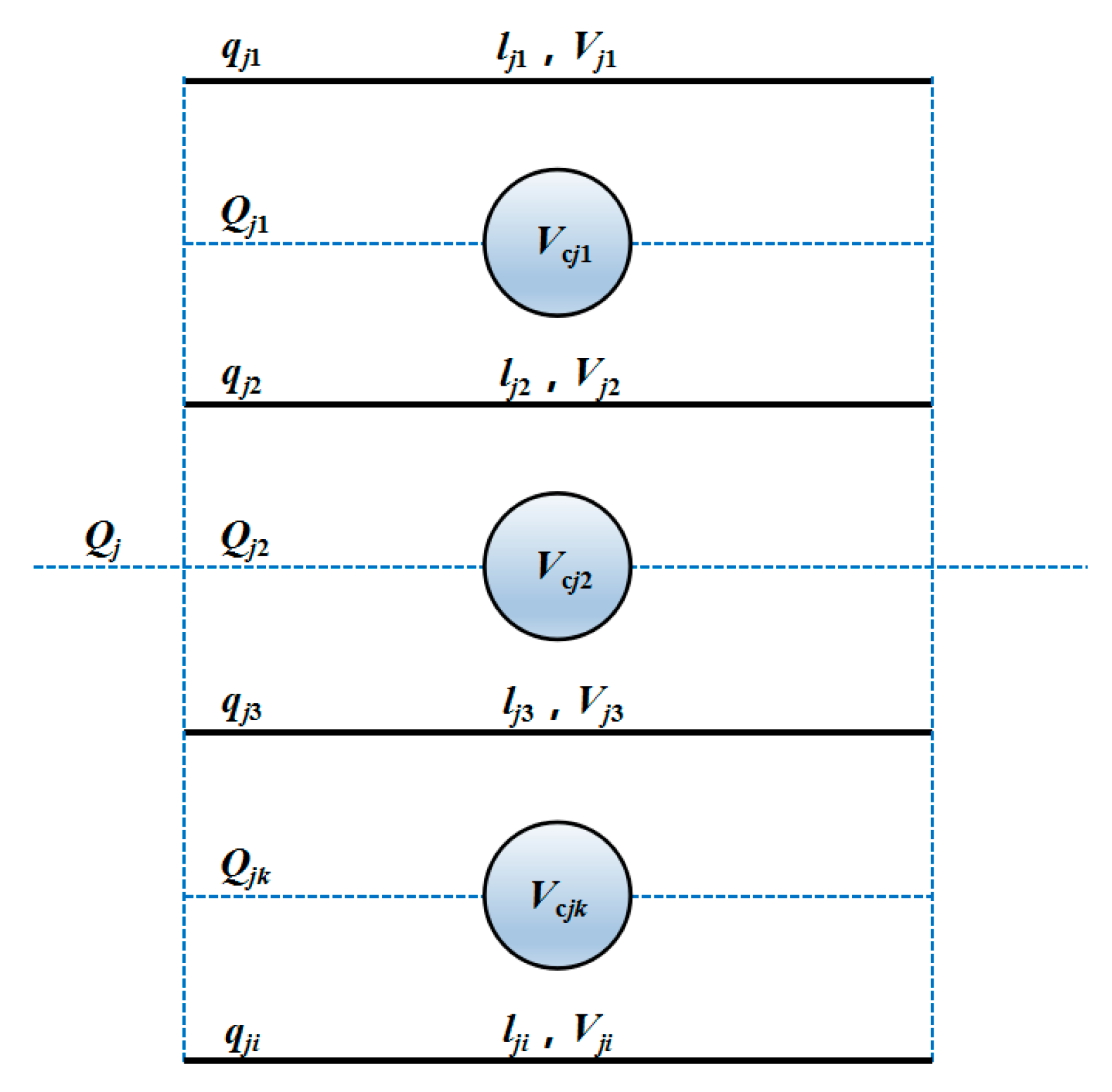
Based on the matching relationship between the fracture-cavity configuration and the tracer curve in fracture-cavity reservoirs and the above assumptions, a physical model of the interwell fracture-cavity structure for tracer migration was established, as shown in Figure 6. There are N parallel branch flow channels (fractures/pipes) in the interwell fracture-cavity composite structure from the water injection well to the jth production well in the injection-production well group, and the volume and length of the ith parallel branch flow channel are Vji and lji, respectively. There are M parallel branch caves, and the volume of the kth branch cave is Vcjk (Figure 6).
3.2. Mathematical Model
From the physical model of the fracture-cavity combination structure between the injection well and production well j, it can be seen that the output concentration of the tracer in the production well should be the superposition of the agent concentration in the production well produced by N parallel branch flow channels and M parallel branch karst caves [26,27,28,29]. In this section, a quantitative interpretation model of tracers with different interwell fracture-cavity configurations is established by deriving the mathematical models of tracer concentration output in parallel branch channels and branch karst caves.
3.2.1. Mathematical Model of Tracer Concentration Output in Parallel Branch Channels
Based on the material balance equation of the tracer transporting in a one-dimensional flow channel with an arbitrary cross-sectional shape, the solution is solved in combination with its fixed solution conditions. After simplification, through dimensional analysis and unit conversion, the analytical solution of the concentration distribution of the Vdji tracer slug in the ith parallel branch flow channel is obtained [26,27,28,29]:
where Cji(t) is the tracer output concentration of the ith parallel flow channel of production well j (mg/L); C0 is the concentration of the tracer slug injected into the injection well (mg/L); Vdji is the volume of tracer slug injected from the injection well to the ith parallel flow channel of production well j (m3); is the average residence time of the tracer from the injection well to the ith parallel flow channel of production well j (d); lji is the length of the flow channel of the ith parallel flow channel from the injection well to production well j (m); Vji is the flow channel volume of the ith parallel flow channel from the injection well to production well j (m3); αji is the hydrodynamic dispersion constant of the ith parallel flow channel tracer from the injection well to the production well (m); and t is the time (d).
For tracer monitoring in mines, the volume and concentration of the tracer solution injected into the injection well can be known. After the tracer is injected, it will be distributed to different parallel bodies in certain proportions. In Formula (1), the injected tracer slug volume Vdji of the ith parallel flow channel in production well j can be allocated by different parallel flow rates; then the volume of the tracer slug distributed to the ith parallel flow channel is
where fj is the distribution coefficient of injected water from the injection well to the production well (f); Vd is the volume of the tracer slug injected by the injection well (m3); qji is the flow rate of the ith parallel channel flow from the injection well to production well j (m3/d); and Qj is the total flow rate from the injection well to the production well j (m3/d).
In this equation,
Substituting Equation (2) into Equation (1), we obtain
Equation (4) is the mathematical model of the tracer concentration output in the ith parallel flow channel from the injection well to the production well j.
3.2.2. Mathematical Model of Tracer Concentration Output in Parallel Branch Caves
Due to the large scale of karst caves, the fluid quickly reaches equilibrium; the specific form of fluid flow cannot be considered, and it is regarded as an equipotential body [35]. The migration of the tracer in a karst cave is dominated by slow diffusion, and the difference in its concentration gradient is not large; the output concentration gradient of the tracer in the cave is equal to the average concentration in the cave, which can be derived according to the equilibrium relationship of the tracer [35]:
where Cin(t) is the concentration of the tracer at the entrance of the cave at time t (mg/L) and is the average residence time of the fluid in the cave (that is, cave volume divided by cave output flow; d).
If we solve Equation (5), let the tracer concentration at the entrance of the cave Cin(t) be the injected tracer slug constant concentration C0, and use the residence time to describe the delayed response of the tracer from the entrance to the exit of the cave, the mathematical model of the tracer concentration output of the kth parallel cave from the injection well to the production well j is
where Cjk(t) is the tracer output concentration of the kth parallel cave in production well j (mg/L); Vdjk is the volume of the tracer slug injected from the injection well to the kth parallel cave of production well j (m3); Vcjk is the volume of the kth parallel cave from the injection well to production well j (m3); and is the average residence time of the tracer in the kth parallel cave from the injection well to production well j (d).
Similar to the solution for the volume of the tracer slug assigned to the parallel branch channel, the volume of the tracer slug assigned to the parallel branch cave is
where qjk is the flow rate from the injection well to the kth parallel karst cave of production well j (m3/d).
In this equation,
Substituting Equation (7) into Equation (6), we obtain
Equation (9) is the mathematical model of the tracer concentration output of the kth parallel cave from the injection well to production well j.
3.2.3. Mathematical Model of Tracer Concentration Output for Fracture-Cavity Reservoirs
The tracer production concentration of fracture-cavity reservoirs should be the superposition of tracer production concentrations of all parallel branch flow channels and branch karst caves at production well j, namely,
where Cj(t) is the tracer output concentration of production well j (mg/L); Nj is the total number of parallel flow channels from the injection well to production well j; Mj is the total number of parallel karst caves from the injection well to production well j; and qjk is the kth parallel from the injection well to production well j.
Substituting Equations (3), (4), (8), and (9) into Equation (10), after simplification, we obtain
In this equation,
Equation (11) is the interwell tracer interpretation model for fracture-cavity reservoirs considering the interwell fracture-cavity configuration. Based on the matching relationship between the mine tracer curve shape and the interwell fracture-cavity configuration, the interwell fracture-cavity combination structure is determined. Nj and Mj in Equation (11) are determined according to the number of fractures and cavities contained in the fracture-cavity combination structure. In Equation (11), the known parameters before fitting are fj (which can be calculated by the semi-quantitative tracer concentration curve method) and Vd, C0, and Cj(t) (which can be detected by tracer field injection and sampling), and the parameters to be optimized are Vcjk, Vji, and lji. Then, the volume Vji and length lji of each parallel branch flow channel and volume Vcjk of each parallel branch karst cave can be obtained by fitting the tracer curve with the above formula. Through further calculations, the section parameters of parallel branch flow channels and the flow of each parallel branch channel and the cave can be obtained. The main sources of the parameters in Formula (11) and the quantitative parameters between wells obtained by fitting the tracer production concentration curve are shown in Table 2.
4. Field Application and Analysis
4.1. Tracer Curve Fitting Method
The inversion and fitting of the tracer concentration curve between wells in fracture-cavity reservoirs can be regarded as a nonlinear optimization problem, as follows [26,27,28,29]:
where Cj(t) is the tracer concentration calculated by the theoretical model in production well j at time t (mg/L); Cj*(t) is the tracer concentration of production well j obtained from the actual measurement of the mine at time t (mg/L); and n is the actual tracer monitoring days of production well j (d).
Since the objective function is an optimization solution to a nonlinear function, an optimization algorithm is usually used to solve this problem. At present, the optimization algorithms commonly used in engineering based on swarm optimization problems include particle swarm optimization (PSO), artificial bee colony (ABC) and ant colony (ACO) algorithms, genetic algorithm (GA), and artificial neural networks (ANN). Each algorithm has its advantages. For example, compared with the traditional algorithm, the particle swarm optimization algorithm has a very fast computation speed and strong global search ability. It is suitable for continuous function extreme value problems and has a strong global search ability for nonlinear and multi-peak problems. Therefore, the particle swarm algorithm is a good choice for the inversion fitting of multimodal tracer curves. This algorithm regards each possible solution of the optimization problem as a “particle” in the search area. The quality of all particles is determined by the fitness of the objective function. The fitness of all particles varies with position and speed; it changes with changes in the relationship, keeps searching in the solution domain with the current optimal particle, and finally obtains the optimal solution to the problem.
4.2. Field Application
To verify the reliability and applicability of the established interwell tracer interpretation model and related calculation methods in fracture-cavity reservoirs, the particle swarm algorithm in 1stOpt software (Beijing, China) [36] was used to analyze fracture-cavity S48 in the fourth block of Tahe Oilfield. The interwell tracer monitoring data of the unit TK411 well group were interpreted, and relative error analysis and an evaluation of the obtained related fitting parameters and extended parameters were carried out. The well group started water injection in May 2005. On 14 April 2007, 14 kg of BY-1 tracer with a designed concentration of 100% was injected into injection well TK411, which lasted for 200 days. A total of 1594 samples were obtained, and 1577 samples were analyzed. A good tracer response curve and dynamic production data were obtained.
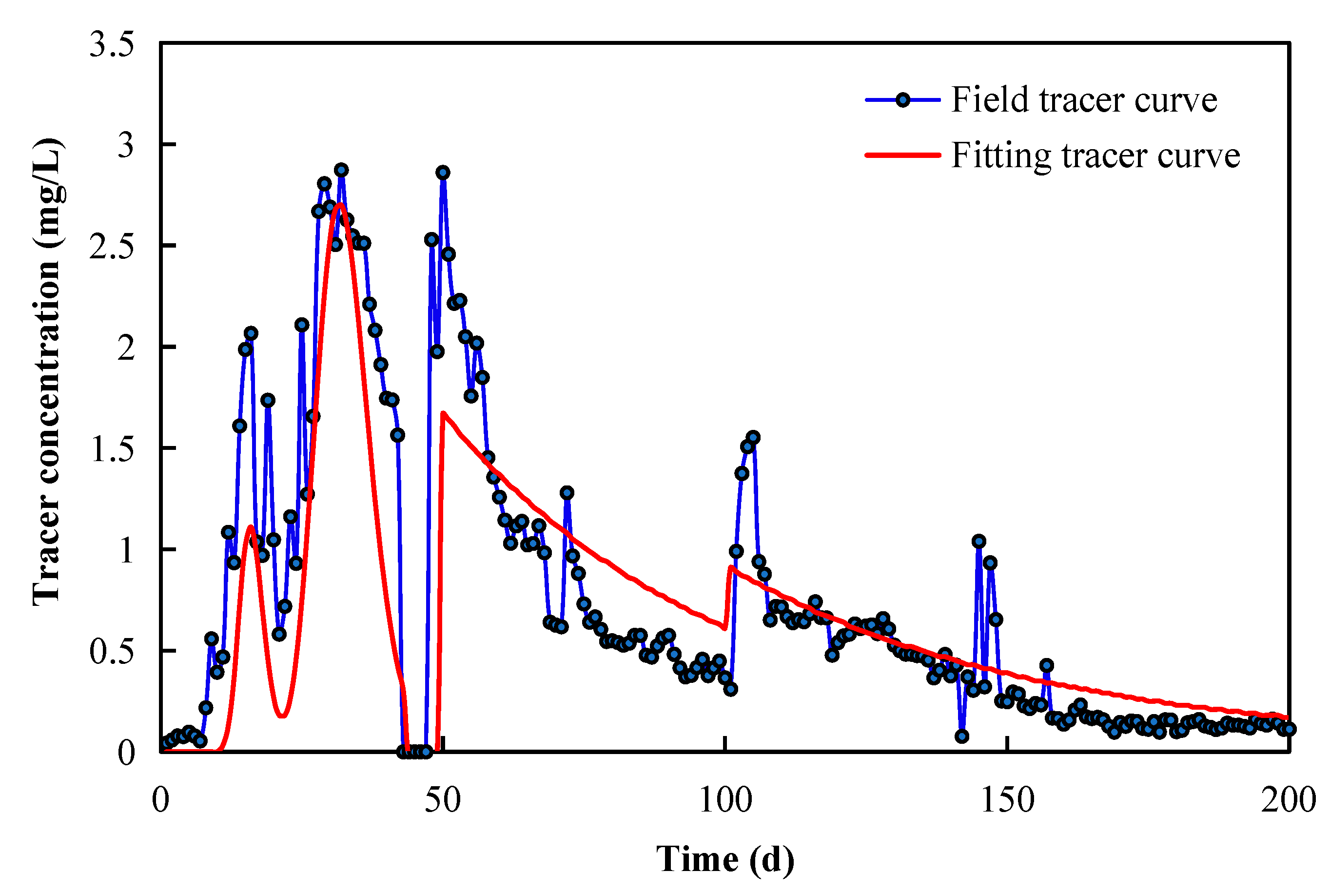
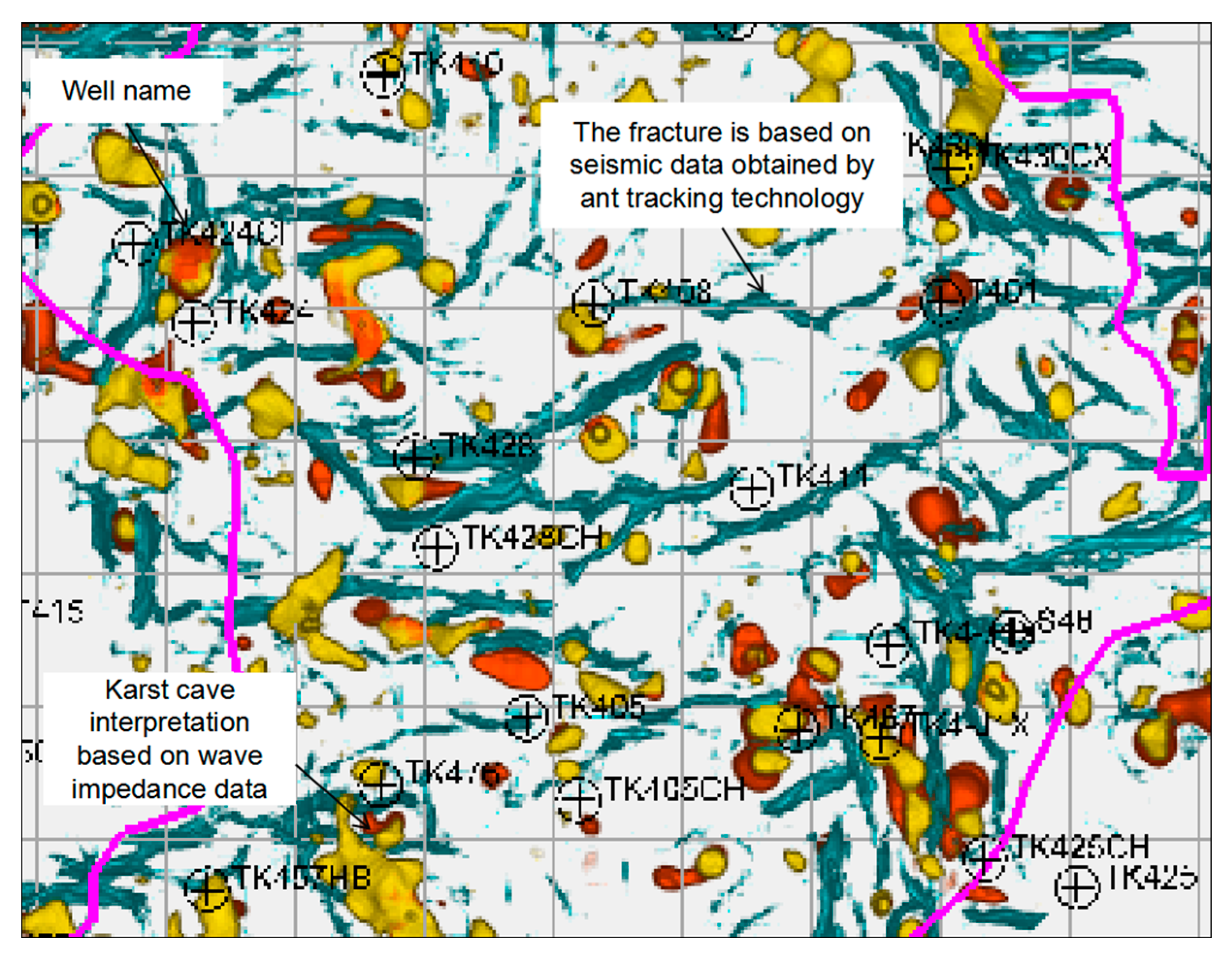
There are eight effective production wells in well group TK411. This time, three wells with multimodal tracer response curves (TK424CH, TK476, and TK457H) were selected as the specific analysis objects. Using the matching relationship between the tracer curve shape and the interwell fracture-cavity configuration in fracture-cavity reservoirs (Table 1), it can be seen that the tracer curve of well TK424CH is a parallel type with two flow channels between wells; the tracer curve of well TK476 shows a single flow channel in parallel with one karst cave interwell fracture-cavity configuration; and the tracer curve of well TK457H shows a two-flow channel in parallel with a two karst cave interwell fracture-cavity configuration (Figure 7, Figure 8, Figure 9 and Figure 10). As can be seen from Figure 10, there are multiple strong amplitude change regions in each path direction from injection well TK411 to production wells TK424CH, TK476, and TK457H, and there is a high probability of multiple flow channels/cavities between wells, which indicates that the recognition of fracture-cavity configuration is reliable.
Using the interwell tracer interpretation model established in this paper (Formula (11)), the particle swarm algorithm was used in 1stOpt software (Beijing, China) to perform three inversions and fittings for the three wells, and the tracer fitting curve of each well was obtained. The agent fitting curve and fitting parameters were obtained, and the corresponding expansion parameters were calculated (Figure 7, Figure 8 and Figure 9, Table 3 and Table 4).
4.3. Results Analysis
As can be seen from Table 5, the absolute error between the sums of the field tracer and fitting tracer concentrations and production wells TK424CH, TK476, and TK457H is 13.50, 15.93, and 15.65 mg/L, respectively, and the relative error is 37.26, 24.89, and 10.44%. The average relative error of the three wells is less than 25%, and the fitting results meet the requirements of field engineering.
It can be seen from Figure 7, Figure 8 and Figure 9 that the shape of the fitting curve can well reflect the fracture-cavity combination structure between wells, and the tracer curve fitting effect for each well is good, which can effectively explain the volume and length of branch flow channels/karst caves (Table 3). To further verify and evaluate the adaptability and reliability of the model, the total flow obtained by tracer interpretation (expanded calculation parameters; Table 4) was compared and verified with the daily water production during the monitoring period of the field tracer. The absolute error between them is not more than 1.6 m3/d, the average absolute error is 0.83 m3/d, and the relative error is not more than 7%. The average relative error is only 3.02%, indicating that the established interpretation model can better reflect the flow between well properties and the resulting fitted direct output parameters and extended computational parameters are reliable (Table 6).
5. Conclusions
- (1)
- Using dynamic and static data of Tahe Oilfield and tracer monitoring curves between wells, the interwell channels can be divided into single-channel and multi-channel types. The matching relationship between the fracture-cavity combination structure of different channel types and the shape of the tracer curve is clarified. The tracer production curve of the interwell fracture/pipe structure shows a regular peak shape with two basically symmetrical wings, and the interwell karst cave structure shows the characteristics of a trailing curve with a steep ascending wing and a slow descending wing. The difference in peak time appearing in the tracer multi-peak curve means that the channel size is different; the main peak often reflects the type of mainstream channel in parallel, and the number of peaks reflects the number of parallel channels.
- (2)
- Based on convective diffusion theory and the basic idea of interwell tracing, a unified quantitative interpretation model of interwell tracers for fracture-cavity reservoirs with an arbitrary fracture-cavity combination structure based on branch flow channels and branch caves is established, and the input parameters required to explain the application of the model, the parameters that can be obtained directly after fitting the tracer curve, and the parameters that can be further expanded based on the output parameters are clarified.
- (3)
- Taking the three wells of well group TK411 in the S48 fracture-cavity unit in the fourth area of Tahe Oilfield as an example, the type of interwell fracture-cavity combination structure was judged by the shape of the tracer curve between wells (determining the number of branch channels and branch karst caves, peak time, etc.) using the established interpretation model with the particle swarm optimization algorithm in 1stOpt software (Beijing, China) to carry out the fitting, interpretation, and reliability evaluation of the tracer curve. The tracer curve fitting effect of each well is good. The comparison and verification of the total flow rate explained by the tracer and the daily water production during the monitoring period of the tracer in the mine show that the average absolute error between them is 0.83 m3/d, and the relative error is only 3.02%, which effectively demonstrates the applicability and reliability of the established tracer interpretation model.
Author Contributions
Author contributions: conceptualization, C.J., G.H. and J.N.; methodology, C.J. and Q.D.; validation, L.L. and Q.D.; data curation, C.J. and G.H.; writing—original draft, C.J., Q.D. and M.G.; writing—review and editing, C.J., L.L. and Q.D. All authors have read and agreed to the published version of the manuscript.
Funding
This study was funded by the National Natural Science Foundation of China (51804256, 52174031, 52004216, 52104032, 52004215, 51704235) and the Natural Science Basic Research Plan in Shaanxi Province of China (No. 2023-JC-YB-433, 2019JQ-287, 2020JQ-787, 2018JQ5208).
Institutional Review Board Statement
Not applicable.
Informed Consent Statement
Not applicable.
Data Availability Statement
Not applicable.
Conflicts of Interest
The authors declare no conflict of interest.
References
- Jiang, H.Y.; Song, X.M.; Wang, Y.J.; An, X.X.; Qi, R.L.; Peng, S.M. Current situation and forecast of the worlds carbonate oil and gas exploration and development. Offshore Oil 2008, 28, 6–13. [Google Scholar]
- Li, Y. Ordovician carbonate fracture-cavity reserovirs identification and quantitative characterization in Tahe Oilfield. J. China Univ. Pet. (Ed. Nat. Sci.) 2012, 36, 1–7. [Google Scholar]
- Huang, S.W.; Zhang, Y.; Zheng, X.P.; Zhu, Q.F.; Shao, G.M.; Cao, Y.Q.; Chen, X.G.; Yang, Z.; Bai, X.J. Types and characteristics of carbonate reservoirs and their implication on hydrocarbon exploration: A case study from the eastern Tarim Basin, NW China. J. Nat. Gas Geosci. 2017, 2, 73–79. [Google Scholar]
- Li, Y.; Kang, Z.J.; Xue, Z.J.; Zheng, S.Q. Theories and practices of carbonate reservoirs development in China. Pet. Explor. Dev. 2018, 45, 712–722. [Google Scholar]
- Dai, C.L.; Fang, J.C.; Jiao, B.L.; He, L.; He, X.Q. Development of the research on EOR for carbonate fractured-vuggy reservoirsin China. J. China Univ. Pet. (Ed. Nat. Sci.) 2018, 42, 67–78. [Google Scholar]
- Yue, P.; Xie, Z.W.; Huang, S.Y.; Liu, H.H.; Liang, S.B.; Chen, X.F. The application of N2 huff and puff for IOR in fracture-vuggy carbonate reservoir. Fuel 2018, 234, 1507–1517. [Google Scholar]
- Trice, R.; C Reservoirs Ltd. Challenges and insights in optimising oil production form middle eastern karst reservoirs. In Proceedings of the SPE Middle East Oil and Gas Show and Conference, Manamah, Bahrain, 12–15 March 2005. [Google Scholar]
- Carpenter, C. Reservoir-surveillance data creates value in fractured-carbonate applications. J. Pet. Technol. 2018, 70, 84–86. [Google Scholar]
- Dittaro, L.M.; Schwindt, C.; Holding, T.L. Surveillance & optimization of a waterflooded fractured carbonate reservoir. In Proceedings of the SPE International Petroleum Technology Conference, Dubai, United Arab Emirates, 4–6 December 2007. [Google Scholar]
- Shbair, A.F.; Hammadi, H.A.; Martinez, J.; Adeoye, O.; Abdou, M.; Saputelli, L.; Bahrini, F. The value of reservoir surveillance-applications to fractured carbonates under waterflooding. In Proceedings of the SPE Abu Dhabi International Petroleum Exhibition & Conference, Abu Dhabi, United Arab Emirates, 13–16 November 2017. [Google Scholar]
- Tian, F.; Di, Q.Y.; Jin, Q.; Cheng, F.Q.; Zhang, W.; Lin, L.M.; Wang, Y.; Yang, D.B.; Niu, C.K.; Li, Y.X. Multiscale geological-geophysical characterization of the epigenic origin and deeply buried paleokarst system in Tahe Oilfield, Tarim Basin. Mar. Pet. Geol. 2019, 102, 16–32. [Google Scholar]
- Wang, X.W.; Yuan, G.; Tian, Y.C.; Lv, L.; Qie, S.H. Analysis of factors affecting carbonate fracture-cave imaging. In Proceedings of the 2013 SEG Annual Meeting, Houston, TX, USA, 22–27 September 2013. [Google Scholar]
- Lai, J.; Peng, X.J.; Xiao, Q.Y.; Shi, Y.J.; Zhang, H.T.; Zhao, T.P.; Chen, J.; Wang, G.W.; Qin, Z.Q. Prediction of reservoir quality in carbonates via porosity spectrum from image logs. J. Pet. Sci. Eng. 2019, 173, 179–208. [Google Scholar]
- Wei, P.; Zhang, T.Y.; Du, J.; Ai, S.; Mao, J. Caves diagnosis in carbonate reservoirs. In Proceedings of the SPE Middle East Oil and Gas Show and Conference, Manama, Bahrain, 18 March 2019. [Google Scholar]
- Wan, Y.Z.; Liu, Y.W.; Chen, F.F.; Wu, N.Y.; Hu, G.W. Numerical well test model for caved carbonate reservoirs and its application in Tarim Basin, China. J. Pet. Sci. Eng. 2018, 161, 611–624. [Google Scholar]
- Yue, P.; Xie, Z.W.; Liu, H.H.; Chen, X.F.; Guo, Z.L. Application of water injection curves for the dynamic analysis of fractured-vuggy carbonate reservoirs. J. Pet. Sci. Eng. 2018, 169, 220–229. [Google Scholar]
- Al-Obathani, O.H.; Al-Wehaibi, B.A.; Al-Thawad, F.M.; Rahman, N.M. New, integrated approach to diagnose, characterize and locate inter-well fracture connectivity in carbonate reservoirs from transient-test data. In Proceedings of the SPE Kingdom of Saudi Arabia Annual Technical Symposium and Exhibition, Dammam, Saudi Arabia, 24–27 April 2018. [Google Scholar]
- Sanni, M.; Abbad, M.; Kokal, S.; Ali, R.; Zefzafy, I.; Hartvig, S.; Huseby, O. Reservoir description insights from an inter-well chemical tracer test. In Proceedings of the SPE Kingdom of Saudi Arabia Annual Technical Symposium and Exhibition, Dammam, Saudi Arabia, 24–27 April 2017. [Google Scholar]
- Tayyib, D.; Al-Qasim, A.; Kokal, S.; Huseby, O. Overview of tracer applications in oil and gas industry. In Proceedings of the SPE Kuwait Oil & Gas Show and Conference, Mishref, Kuwait, 13–16 October 2019. [Google Scholar]
- Xie, J.X.; Liu, Z.; Cheng, B.Q.; Wang, C.L.; Yu, Y.C. Tracer technology used in sandstone reservoir and fractured carbonate reservoir. Well Logging Technol. 2008, 32, 272–276. [Google Scholar]
- Li, X.B.; Peng, X.L.; Shi, Y.; Yang, W.M. Application of interwell tracer testing in fracture-cavity reservoirs. J. Oil Gas Technol. 2008, 30, 271–274. [Google Scholar]
- Zhou, L.M.; Guo, P.; Liu, J.; Liu, L.N. Study on inter well connectivity of carbonate rock reservoir with fractures and caves by tracer in Tahe oilfield, Xinjiang, China. J. Chengdu Univ. Technol. (Sci. Technol. Ed.) 2015, 42, 212–217. [Google Scholar]
- Zhang, Z.W.; Cheng, Z.Q.; Gao, C.C.; Ren, S.Y. Tracing detection study on underground reservoir capacity in karst depression area. Geotech. Investig. Surv. 2016, 44, 44–50. [Google Scholar]
- Morales, T.; Valderrama, I.F.; Uriarte, J.A.; Antigüedad, I.; Olazar, M. Predicting travel times and transport characterization in karst conduits by analyzing tracer-breakthrough curves. J. Hydrol. 2006, 334, 183–198. [Google Scholar] [CrossRef]
- Dewaide, L.; Bonniver, I.; Rochez, G.; Hallet, V. Solute transport in heterogeneous karst systems: Dimensioning and estimation of the transport parameters via multi-sampling tracer-tests modelling using the OTIS (One-dimensional Transport with Inflow and Storage) program. J. Hydrol. 2016, 534, 567–578. [Google Scholar] [CrossRef]
- Zou, N.; Huang, Z.J.; Li, X.N. Research on Single Pipe Tracer Output Model in Inter-well Trapezoidal Reservoirs. In Proceedings of the International Field Exploration and Development Conference, Qingdao, China, 20–22 October 2021; pp. 3050–3057. [Google Scholar]
- Zou, N.; Huang, Z.J.; Ma, G.R.; Wang, Q.; Lin, J.E.; Jing, C. Classified Equivalent Interpretation Model for Interwell Tracer in Fractured-Vuggy Reservoir and Its Application. J. Xi’an Shiyou Univ. (Nat. Sci. Ed.) 2021, 36, 52–58. [Google Scholar]
- Jing, C.; Pu, C.S.; He, Y.L.; Gu, X.Y.; Liu, H.Z.; Cui, S.X. Tracer production model of single fracture belt and analysis parameters sensitivity. Well Logging Technol. 2016, 40, 408–412. [Google Scholar]
- Jing, C.; Pu, C.S.; Gu, X.Y.; He, Y.L.; Wang, B.; Cui, S.X. Classification and interpretation models of inter-well chemical tracer monitoring for fractured ultra-low permeability oil reservoirs. Oil Drill. Prod. Technol. 2016, 38, 226–231. [Google Scholar]
- Luhmann, A.J.; Covington, M.D.; Alexander, S.C.; Chai, S.Y.; Schwartz, B.F.; Groten, J.T.; Alexander, E.C., Jr. Comparing conservative and nonconservative tracers in karst and using them to estimate flow path geometry. J. Hydrol. 2012, 448–449, 201–211. [Google Scholar]
- Ji, S.S.; Liu, J.G.; Wu, Y.; Peng, D.W.; Zhang, B.L.; Wang, M.X. Comparative study on characteristics of tracer curve laboratory experiment of karst pipeline and karst fracture. Site Investig. Sci. Technol. 2017, 4, 11–14+25. [Google Scholar]
- Borghi, A.; Renard, P.; Cornaton, F. Can one identify karst conduit networks geometry and properties from hydraulic and tracer test data? Adv. Water Resour. 2016, 90, 99–115. [Google Scholar]
- Pu, C.S.; Jing, C.; He, Y.L.; Gu, X.Y.; Zhang, Z.Y.; Wei, J.K. Multistage interwell chemical tracing for step-by-step profile control of water channeling and flooding of fractured ultra-low permeability reservoirs. Pet. Explor. Dev. 2016, 43, 621–629. [Google Scholar]
- Rong, Y.S.; Pu, W.F.; Zhao, J.Z.; Li, K.X.; Li, X.H.; Li, X.B. Experimental research of the tracer characteristic curves for fracture-cave structures in a carbonate oil and gas reservoir. J. Nat. Gas Sci. Eng. 2016, 31, 417–427. [Google Scholar] [CrossRef]
- Jing, C.; Zhang, S.; Li, L.; Wang, J.; Chen, B.; Tian, B.; Dai, Z.Y.; Gao, L. Rapid Identification of Interwell Fracture Cavity Combination Structure in Fracture-Cavity Reservoir Based on Tracer-Curve Morphological Characteristics. Front. Energy Res. 2022, 10, 892622. [Google Scholar]
- 1stOpt, 9.0, 7D-Soft High Technology Inc.: Beijing, China, 2020. Available online: http://www.7d-soft.com/(accessed on 6 July 2021).
Figure 1.
(a) Interwell fracture/pipe diagram; (b) tracer curve of well TK455.

Figure 2.
(a) Interwell karst cave diagram; (b) tracer curve of well TK401.

Figure 3.
(a) Interwell parallel pipe/fracture diagram; (b) tracer curve of well TK719CH.

Figure 4.
(a) Interwell parallel pipe/fracture diagram; (b) tracer curve of well TK467.

Figure 5.
(a) Interwell parallel pipe/fracture diagram; (b) tracer curve of well TK457.

Figure 6.
Schematic diagram of physical model of interwell fracture-cavity structure.

Figure 7.
Fitting result of tracer concentration curve of well TK424CH.

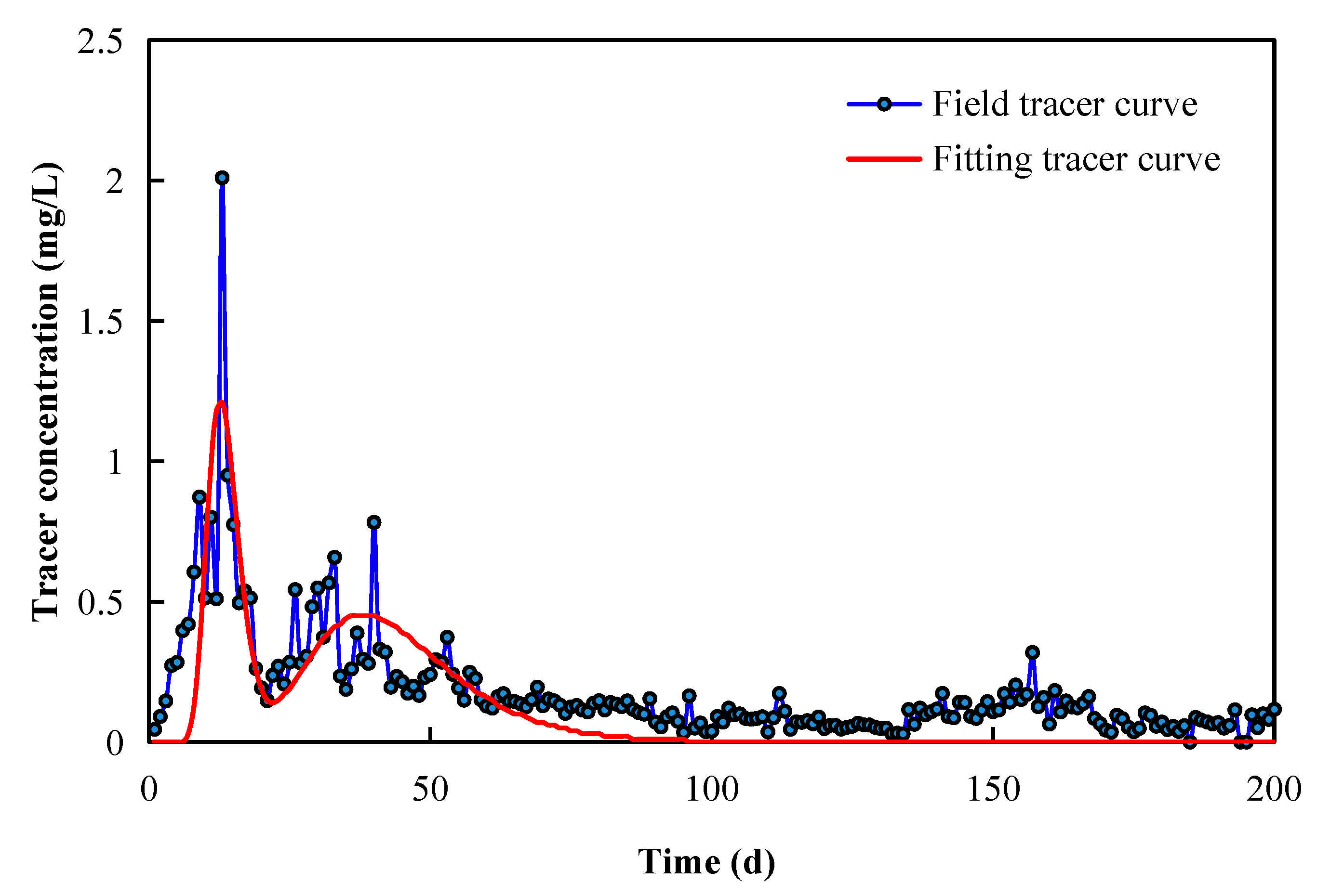
Figure 8.
Fitting result of tracer concentration curve of well TK476.

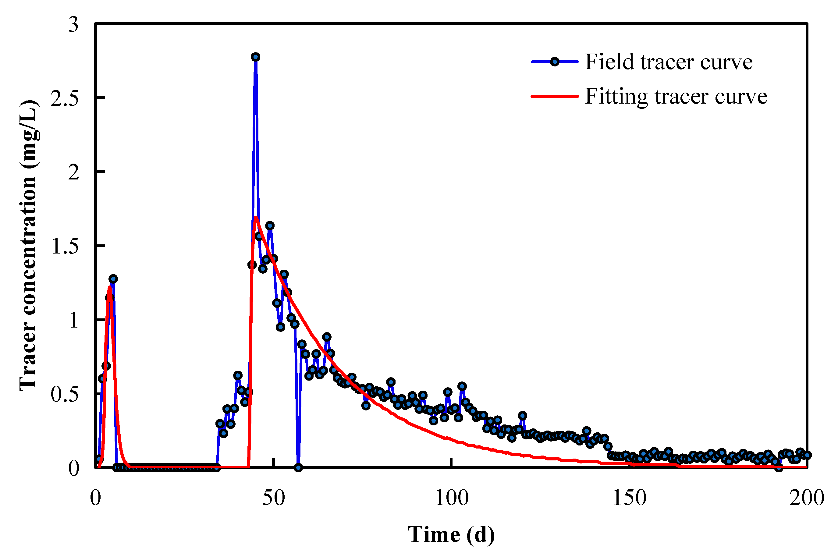
Figure 9.
Fitting result of tracer concentration curve of well TK457H.

Figure 10.
Seismic multi-attribute plane superposition 0–80 ms below plane T74.


Table 1.
Classification characteristics of interwell tracer curve in fracture-cavity reservoir [35].
Table 1.
Classification characteristics of interwell tracer curve in fracture-cavity reservoir [35].
| Serial Number | Peak Pattern | Number of Peaks | Characteristics of Two Wings | Fracture-Cavity Combination Pattern | Curve Shape |
|---|---|---|---|---|---|
| 1 | Single sharp peak | 1 | Basic symmetry | Single fracture |  |
| Single pipe | |||||
| 2 | Single slow peak | 1 | Ascending branch: steep Descending branch: slow Trailing phenomenon: obvious | Single cavity |  |
| Fracture series cavity | |||||
| Pipe series cavity | |||||
| 3 | Multiple peaks | Multiple independent peaks | Two wings of each peak: basically symmetrical | Multiple fractures in parallel (Flow difference: large) |  |
| Multiple pipes in parallel (Flow difference: large) | |||||
| Two wings of each peak: Ascending branch: steep Descending branch: slow | Multiple cavities in parallel (Flow difference: large) |  | |||
| Multiple continuous peaks | Upper half peak: symmetry Descending branch: trailing Continuous peak duration: short | Multiple fractures in parallel (Flow difference: small) |  | ||
| Multiple pipes in parallel (Flow difference: small) | |||||
| Upper half peak: basic symmetry Descending branch: trailing obviously Continuous peak duration: long | Multiple cavities in parallel (Flow difference: small) |  |
Table 2.
Input and output parameters of interwell tracer interpretation model for fracture-cavity reservoirs.
Table 2.
Input and output parameters of interwell tracer interpretation model for fracture-cavity reservoirs.
| Model Parameters Type | Parameters Acquisition Method | Specific Parameters |
|---|---|---|
| Model input parameters | Tracer concentration curve semi-quantitative calculation parameters | Distribution coefficient of injected water |
| Average residence time of each parallel branch channel and cave | ||
| Tracer monitoring for direct access to parameters | Tracer injection slug volume and concentration | |
| Tracer output concentration data | ||
| Tracer monitoring time data | ||
| Model output parameters | Direct fit of model to output parameters | Volume of each parallel branch channel and cave |
| Length of each parallel branch runner | ||
| Extended calculation to obtain parameters | Section parameters of each parallel branch flow channel (area, equivalent diameter) | |
| Total flow, flow of each parallel branch channel and cave | ||
| Average true velocity of fluid in each parallel branch channel |
Table 3.
Tracer interpretation results (fitting direct output parameters).
| Well Name | Fit Number | Branch Channel/Cave Volume (m3) | Total Volume (m3) | Branch Channel Length (m) | Running Time (s) | ||||
|---|---|---|---|---|---|---|---|---|---|
| Flow Channel 1 | Flow Channel 2 | Cave 1 | Cave 2 | Flow Channel 1 | Flow Channel 2 | ||||
| TK424CH | 1st | 150.09 | 480.14 | — | — | 630.23 | 2827.07 | 1817.33 | 12 |
| 2nd | 141.62 | 497.75 | — | — | 639.37 | 2885.18 | 1820.68 | 10 | |
| 3rd | 148.42 | 467.74 | — | — | 616.16 | 2795.53 | 1833.05 | 13 | |
| TK476 | 1st | 63.48 | — | 750.3 | — | 813.78 | 2796.66 | — | 55 |
| 2nd | 71.72 | — | 749.22 | — | 820.94 | 2529.78 | — | 66 | |
| 3rd | 70.71 | — | 754.58 | — | 825.29 | 2778.98 | — | 57 | |
| TK457H | 1st | 69.50 | 602.80 | 353.77 | 50.05 | 1076.12 | 3932.93 | 3474.56 | 213 |
| 2nd | 74.54 | 543.07 | 364.42 | 61.73 | 1043.76 | 3707.29 | 3001.19 | 279 | |
| 3rd | 60.94 | 631.57 | 350.05 | 63.60 | 1106.16 | 3958.92 | 3216.67 | 216 | |
Table 4.
Tracer interpretation results (extended calculation parameters).
| Well Name | Fit Number | Branch Channel Cross-Sectional Area (m2) | Branch Flow Channel/Cave Flow (m3/d) | Total Flow (m3/d) | |||||
|---|---|---|---|---|---|---|---|---|---|
| Flow Channel 1 | Flow Channel 2 | Flow Channel 1 | Flow Channel 2 | Cave 1 | Cave 2 | Each | Average | ||
| TK424CH | 1st | 0.053 | 0.264 | 11.55 | 12.00 | — | — | 23.55 | 23.33 |
| 2nd | 0.049 | 0.273 | 10.89 | 12.44 | — | — | 23.34 | ||
| 3rd | 0.053 | 0.255 | 11.42 | 11.69 | — | — | 23.11 | ||
| TK476 | 1st | 0.023 | — | 15.87 | — | 17.45 | — | 33.32 | 34.63 |
| 2nd | 0.028 | — | 17.93 | — | 17.42 | — | 35.35 | ||
| 3rd | 0.025 | — | 17.68 | — | 17.55 | — | 35.23 | ||
| TK457H | 1st | 0.018 | 0.173 | 4.34 | 18.84 | 7.08 | 0.48 | 30.73 | 30.46 |
| 2nd | 0.020 | 0.181 | 4.66 | 16.97 | 7.29 | 0.59 | 29.51 | ||
| 3rd | 0.015 | 0.196 | 3.81 | 19.74 | 7.00 | 0.61 | 31.15 | ||
Table 5.
Error analysis of tracer curve fitting results.
| Well Name | Sum of Field Tracer Concentrations (mg/L) | Sum of Fitted Tracer Concentrations (mg/L) | Absolute Error (mg/L) | Relative Error (%) | Average Relative Error (%) |
|---|---|---|---|---|---|
| TK424CH | 36.23 | 22.73 | 13.50 | 37.26 | 24.20 |
| TK476 | 64.00 | 48.07 | 15.93 | 24.89 | |
| TK457H | 149.91 | 134.26 | 15.65 | 10.44 |
Table 6.
Reliability evaluation of tracer interpretation results.
| Well Name | Average Daily Water Production during Monitoring Period (m3/d) | Extended Calculation of Total Flow (m3/d) | Absolute Error (m3/d) | Relative Error (%) | Average Relative Error (%) |
|---|---|---|---|---|---|
| TK424CH | 24.88 | 23.33 | 1.55 | 6.23 | 3.02 |
| TK476 | 33.72 | 34.63 | 0.91 | 2.70 | |
| TK457H | 30.50 | 30.46 | 0.04 | 0.13 |
Disclaimer/Publisher’s Note: The statements, opinions and data contained in all publications are solely those of the individual author(s) and contributor(s) and not of MDPI and/or the editor(s). MDPI and/or the editor(s) disclaim responsibility for any injury to people or property resulting from any ideas, methods, instructions or products referred to in the content. |
© 2023 by the authors. Licensee MDPI, Basel, Switzerland. This article is an open access article distributed under the terms and conditions of the Creative Commons Attribution (CC BY) license (https://creativecommons.org/licenses/by/4.0/).
Share and Cite
MDPI and ACS Style
Jing, C.; Duan, Q.; Han, G.; Nie, J.; Li, L.; Ge, M. Quantitative Interpretation Model of Interwell Tracer for Fracture-Cavity Reservoir Based on Fracture-Cavity Configuration. Processes 2023, 11, 964. https://doi.org/10.3390/pr11030964
AMA Style
Jing C, Duan Q, Han G, Nie J, Li L, Ge M. Quantitative Interpretation Model of Interwell Tracer for Fracture-Cavity Reservoir Based on Fracture-Cavity Configuration. Processes. 2023; 11(3):964. https://doi.org/10.3390/pr11030964
Chicago/Turabian StyleJing, Cheng, Qiong Duan, Guangshun Han, Jianfeng Nie, Lu Li, and Mingxu Ge. 2023. "Quantitative Interpretation Model of Interwell Tracer for Fracture-Cavity Reservoir Based on Fracture-Cavity Configuration" Processes 11, no. 3: 964. https://doi.org/10.3390/pr11030964
Note that from the first issue of 2016, this journal uses article numbers instead of page numbers. See further details here.