
Inventory Model with Stochastic Demand Using Single-Period Inventory Model and Gaussian Process


1
Department of Electrical and Computer Engineering, Universidad Autónoma de Ciudad Juárez, Ciudad Juárez 32310, Mexico
2
Department of Industrial Engineering and Manufacturing, Universidad Autónoma de Ciudad Juárez, Ciudad Juárez 32310, Mexico
3
Department of Physics and Mathematics, Universidad Autónoma de Ciudad Juárez, Ciudad Juárez 32310, Mexico
*
Author to whom correspondence should be addressed.
†
These authors contributed equally to this work.
Processes 2022, 10(4), 783; https://doi.org/10.3390/pr10040783
Submission received: 20 September 2021
/
Revised: 12 November 2021
/
Accepted: 15 April 2022
/
Published: 16 April 2022
(This article belongs to the Section Process Control and Monitoring)
Abstract
:Proper inventory management is vital to achieving sustainability within a supply chain and is also related to a company’s cash flow through the funds represented by the inventory. Therefore, it is necessary to balance excess inventory and insufficient inventory. However, this can be difficult to achieve in the presence of stochastic demand because decisions must be made in an uncertain environment and the inventory policy bears risks associated with each decision. This study reports an extension of the single-period model for the inventory problem under uncertain demand. We proposed incorporating a Gaussian stochastic process into the model using the associated posterior distribution of the Gaussian process as a distribution for the demand. This enables the modeling of data from historical inventory demand using the Gaussian process theory, which adapts well to small datasets and provides measurements of the risks associated with the predictions made. Thus, unlike other works that assume that demand follows an autoregressive or Brownian motion model, among others, our approach enables adaptability to different complex forms of demand trends over time. We offer several numerical examples that explore aspects of the proposed approach and compare our results with those achieved using other state-of-the-art methods.
1. Introduction
The management of supply chain inventory is crucial to achieving sustainability and is related to a company’s cash flow through the funds represented by the inventory. Excess inventory is generally a symptom of bad managerial practices and can lead to several problems, such as higher storage costs, inventory obsolescence, and the need for more floor space. Conversely, insufficient inventory can increase the probability of unfulfilled demand, costing a company its clients and business reputation. Therefore, when a company’s inventory model prompts orders inaccurately, the company is left with more inventory than needed to meet market demand. In addition, market demand might decrease after the inventory has been supplied. This phenomenon affects companies with perishable inventories of finished goods. Inventories of perishable goods are commonly managed using single-period inventory control; thus, this is known as the single-period problem (SPP) or the “news vendor” problem [1]. Here, we are interested in controlling the inventory of a single item with a stochastic demand model over a single period.
A review of the state of the art regarding SPP shows that much of the research on the topic is related to demand models that do not satisfy the assumptions of a specific probability distribution with known parameters. Factors that make it difficult to accurately characterize demand include limited and unreliable historical data and lack of such data. In this regard, Ref. [2] identified two research lines: the first relies on known demand distribution with unknown parameters, and the second relates to scenarios in which partial information regarding demand distribution, such as some parameters, is available, but the form of the distribution is unknown. Here, we consider the latter research line. Along this line, the work [3] considered a single-period and single-item problem when the demand was assumed to be Markov-modulated. Under this circumstance, they proposed estimating the demand parameters using the earlier result achieved by [4], assuming that for stationary demand with sufficiently high intensity of the arrival process and an extensive duration period, the demand could be considered a normal random variable. Therefore, they could estimate the mean and variance of the number of arrivals during the period. One limiting aspect of this approach is the necessity of having a large sample of historical data to approximate the model parameters.
In another approach [5], the authors proposed a new distributionally robust fuzzy optimization method for the SPP. They characterized the uncertain market demand using a generalized parametric interval-valued possibility distribution. In [6], the authors investigated the SPP using the uncertainty theory [7]. Under this scheme, demand was assumed to be an uncertain variable, and two identification functions of demand were proposed to determine the optimal order quantity that maximizes the expected profit. The uncertainty in their model can be subjective, proposing the use of experts when there are few historical records. In [8], the authors proposed and integrated a decision model that determines the optimal quantities of a single-period product with fuzzy logic. To solve the model, they used a genetic algorithm with a dynamically adaptive penalty. Concerning prediction of demand, in [9], the authors proposed using past demand information and information on characteristics that could be relevant. In this way, and using a linear programming algorithm, the optimal order quantity was learned. This method was based on minimizing the empirical risk. The authors demonstrated their algorithm in relation to nurse staffing in a hospital emergency operating room using two features, the number and type of cases, to predict the required operating room time. This machine-learning approach of incorporating additional features of information has been employed by several other authors [10,11]. For example, in [12], the authors used large data sets to investigate solution methods based on machine learning and quantile regression models to make decisions under the news vendor method.
In the present work, we are interested in the single-period inventory problem in which the distribution of market demand is uncertain. From the literature review, historical data were used to estimate demand behavior; therefore, in this work, we propose using these historical data to characterize demand using the Gaussian process (GP) regression model [13]. Next, we propose using the predictive GP probabilities as the data distribution and incorporate said distribution into the SPP model, similar to [9]. The proposed model can incorporate other attributes of the entire process rather than only information about demand; however, that is not explored here. The main contributions of the paper can be summarized as follows.
- We use the GP to model demand, enabling demand prediction, even if the data are complex or there is not a large amount of historical data.
- We model the demand distribution as a posterior predictive function of the GP, enabling easy, clean integration with the SPP model.
- We report examples using the proposed model.
These aspects allow the proposed approach to adapt to different complex forms of demand trends over time, unlike other works that assumed that demand follows an autoregressive (AR) or Brownian motion model. A list of abbreviations used throughout the article is listed in Table 1.
2. Background
2.1. Gaussian Process
GPs are frequently employed as priors that help specify distributions over spaces of functions and provide flexible non-parametric models whose structures can be specified by choices regarding their main statistics. This enables the balancing of model complexity and reconstruction errors [14]. Thus, GPs are specified by a mean function and a covariance function . GPs can be denoted as and provide a distribution on functions f for which any finite samples have a joint Gaussian distribution [15], i.e., given and a finite set of input points the vector has a multivariate normal distribution.
In most applications, the mean function is left constant, leaving a choice regarding only the covariance function. This function determines several properties of functions sampled from a GP, such as smoothness and periodicity. Generally, the covariance function is also used to define nearness or similarity between samples, and in this way, it models certain processes; thus, the covariance function defines the structure of the GP [13]. For example, a commonly used covariance function is the squared exponential, defined as
where d denotes the Euclidean distance function, and l denotes the scale parameter. Another example is the exponential sine-squared kernel or periodic kernel:
where p corresponds to the periodicity of the kernel, l denotes the length scale and d is the Euclidean distance.
From the covariance function , we can compute the covariance matrix whose entries are ; covariance matrices must be symmetric and positive semidefinite.
2.2. Single-Period Model
The single-period model’s objective function with order quantity y for a one period random demand D can be expressed as the expected cost [16]:
where is the cost, is the holding cost per held unit during the period, is the penalty cost per shortage unit in the period, is the pdf of the demand, and is the expectation value. Please note that there exist other equivalent forms and extensions for (3) [17,18]. Here, we assumed that the demand occurs instantaneously when the period starts and that there is not setup cost.
3. Research Methodology
In this section, we develop the mathematical model of our proposal. We start by modeling demand as a GP. Then, we obtain an expression for its distribution, which we use to evaluate the solution of the SPP. Finally, we design three experiments to test and compare the proposed model with other models.
3.1. Demand as a Gaussian Process
In this section, demand is modeled as a GP, from which we can obtain an expression for the demand distribution. In Equation (3), the desired stochastic behavior is determined by the pdf represented by . Then y is selected according to a probable value of demand, which is used to estimate the expected value of the chosen distribution. We propose to model the distribution of demand D as a GP posterior:
where denotes a GP [13], and the noise is assumed to be independent and identically distributed
where and are the mean and covariance function of the process, respectively. As covariance function, any positive function can be used [19]. Given a dataset of n previous observations, the distribution function of z at given is called the GP posterior and is expressed as
where and
are the posterior mean and variance, respectively, with
and
is an covariance matrix on the dataset .
3.2. Extension to the SPP Model
According to the development in Section 3.1, a robust forecasting method was obtained to model the trend in demand using GPs. This forecast is summarized in the posterior distribution of the demand process under a GP prior. By incorporating this distribution into the SPP model, we can obtain a closed expression of the model’s solution. The proposed model is given as follows:
where the density in (9) is the GP posterior (6), and , are given by Equations (7) and (8), respectively. The optimal value that maximizes the expected profit is now the critical fractile on , given by
with denoting the inverse of the cumulative distribution function of the posterior density . The Equation (10) has the same form as other works [20,21], but the difference is that the distribution is estimated as the posterior distribution of a GP that can be adapted to different forms of complex demand. Unlike [20], which assumes an AR demand process, or in [21] with fuzzy demand, in the proposed model, it is not necessary to assume a specific distribution because using the GP formulation allows the combination of a prior distribution over function spaces and demand data models. This adaptability is accomplished by fitting hyperparameters that control the shape of the GP. This is an important advantage since it is one of the main problems identified in the literature [2,3,5].
In addition, with the incorporation of the GP prior, the resulting model is not limited to one-dimensional time series; other series can be incorporated to estimate demand, i.e., other behaviors related to a specific product demand can be included. Furthermore, additional time series that have a causal relationship can be considered supplemental information, as well as other different trends that momentarily affect the main product demand.
3.3. Numerical Examples
This section presents the design of the numerical examples to evaluate the proposed method. We assumed different representations of the demand to observe the adaptability of the proposed method to these settings.
3.3.1. Demand as an ARMA Process
In this experiment, the demand was modeled as an autoregressive moving-average (ARMA) process. The results of the proposed method in this setting were compared with the method of assuming a uniform distribution, estimating its mean and variance from historical data. We call this the normal estimation method (NSM).
We chose an ARMA process to model the daily demand of some products [22,23]; the AR parameters were given by (0.75, −0.25), and the moving-average (MA) parameters were (0.65, 0.035).
The kernel of the GP used in the proposed model is a combination of the constant kernel and the Matern kernel; their respective hyperparameters were adjusted automatically using the scikit-learn software library [24]. Choosing the correct kernel for a given application is one of the main challenges in using GP-based models. We observed the following heuristics for our selection. The constant kernel modifies the mean of the GP so it can adjust the process with means different from zero. The Matern kernel is a stationary kernel and is parameterized by a length scale parameter of l. This permits adjusting the GP to the scale of the process at hand. The Matern kernel also has an additional parameter, v, which controls the smoothness of the resulting function to adjust to the noise level of the process to model. The Matern kernel is given by [13]
where is the Gamma function, is a modified Bessel function [25], and d is the Euclidean distance between x and y.
Thus, the kernel used for experiments is given by the combination of the constant and Matern kernel:
where c is a constant, as previously stated, and the kernel hyperparameters (constant and Matern) were adjusted automatically by learning from data.
For the NSM, we employed uniform distribution as the pdf of the demand, which is updated day by day based on historical data (10 days) and using a range given by where , are the minimum and maximum quantity requested in the historical data. In the experiments we run 20 realizations of the demand model (ARMA) consisting of 60 days.
3.3.2. Demand as an AR Process
As a second example, we considered a problem with demand modeled as an AR process: the unit purchase price was , the unit sale cost was , holding cost per held unit was , and a penalty cost per shortage unit was . We simulated 150 periods of an AR process of order 1, with a parameter of , a constant of 300, and white noise as the error term, with a variance of . In each period, the quantity to be ordered was estimated; for this, the ARUS method and the proposed method were used. For both methods, it was assumed that there was a demand history of 100 periods, so only the last 50 periods of the simulated total were evaluated. In the estimation with the ARUS method, the exact formula for estimation was used because it is an AR (1) process; for the proposed method, the same kernel of the previous experiment was used.
3.3.3. Demand as Brownian Motion
As a third experiment, the adaptability of the proposed model is illustrated, and the previous setting was again considered, but with demand modeled as a Brownian motion as in [26]. The volatility was set to and the drift parameter to . For the proposed method, the same kernel was used.
4. Results
In this section, we present the experimental results, their interpretations, and the experimental conclusions that can be drawn.
4.1. Example with ARMA
Here, we present the results of a particular realization of demand as an ARMA process. For this realization, we evaluated the models each day; the results can be found in Figure 1a, from which it is observed that the quantity of inventory considering the proposed model had similar behavior to the NSM; both were close to the real demand and did not exceed it.
The estimate of surplus units is shown in Figure 1b. As can be seen in the graph, it is clear that in using the NSM method, there was an excess of inventory with respect to the proposed method, with a peak of almost 100 units more on day 23.
Figure 1c shows the number of shortage units during the period simulated. Please note that the NSM model reached several peaks, e.g., on days 11 and 57, where it exceeded the proposed method by more than 80 shortage units. This is a significant difference if associated costs are considered.
Figure 1d shows box plots to indicate the concentration levels of the inventory in both models and perform the analysis to conclude on the matter. It can be observed that for the proposed model, the inventory quantities had less dispersion than the NSM model, and the levels were on average lower than 100 units, approximately. This means that according to the behavior over time, the estimate of the inventory quantity in 50% of the considered time was close to the value of 100, while in the NSM model, this was exceeded and presented greater dispersion.
4.2. Example with AR
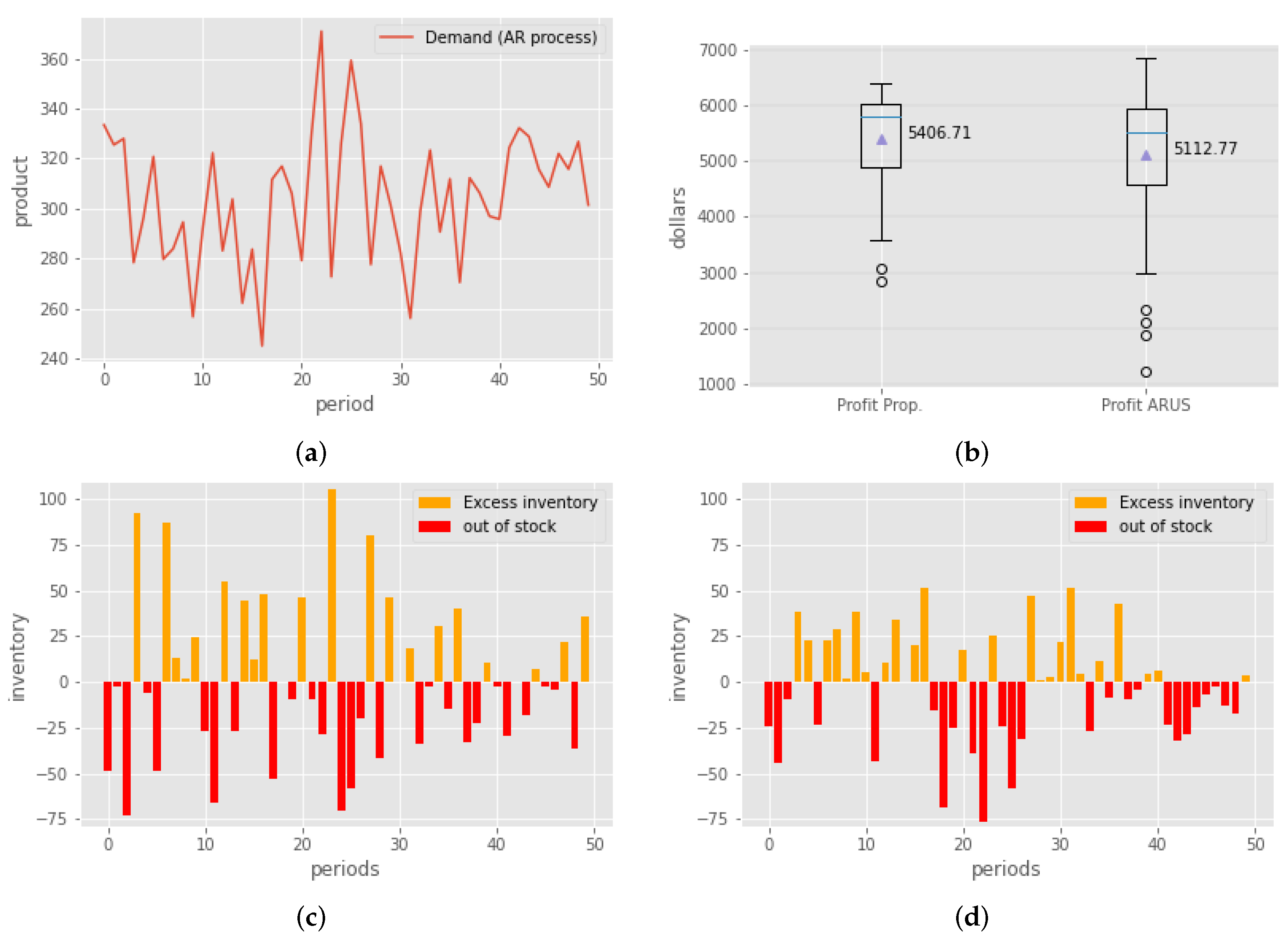
Figure 2a shows the behavior of the demand under the AR assumption for periods 1–50. Figure 2b is a bar graph showing the behavior of the inventory using the ARUS method, while Figure 2d shows the bar graph of the inventory using the proposed method. From the figures, it can be seen that in general the proposed method had better performance with a lower excess of inventory per period; however, in the lack of inventory, it reached the maximum peak between the two methods, but in general, the performance was comparable with that of the ARUS method. Figure 2b, shows a summary of the profit with both methods, the profit with the proposed method had less variance and its median only slightly exceeded that of the ARUS method; however, it should be noted that the ARUS method assumed an AR demand while the proposed method was adaptable without assuming an AR trend.
4.3. Example with Brownian Motion
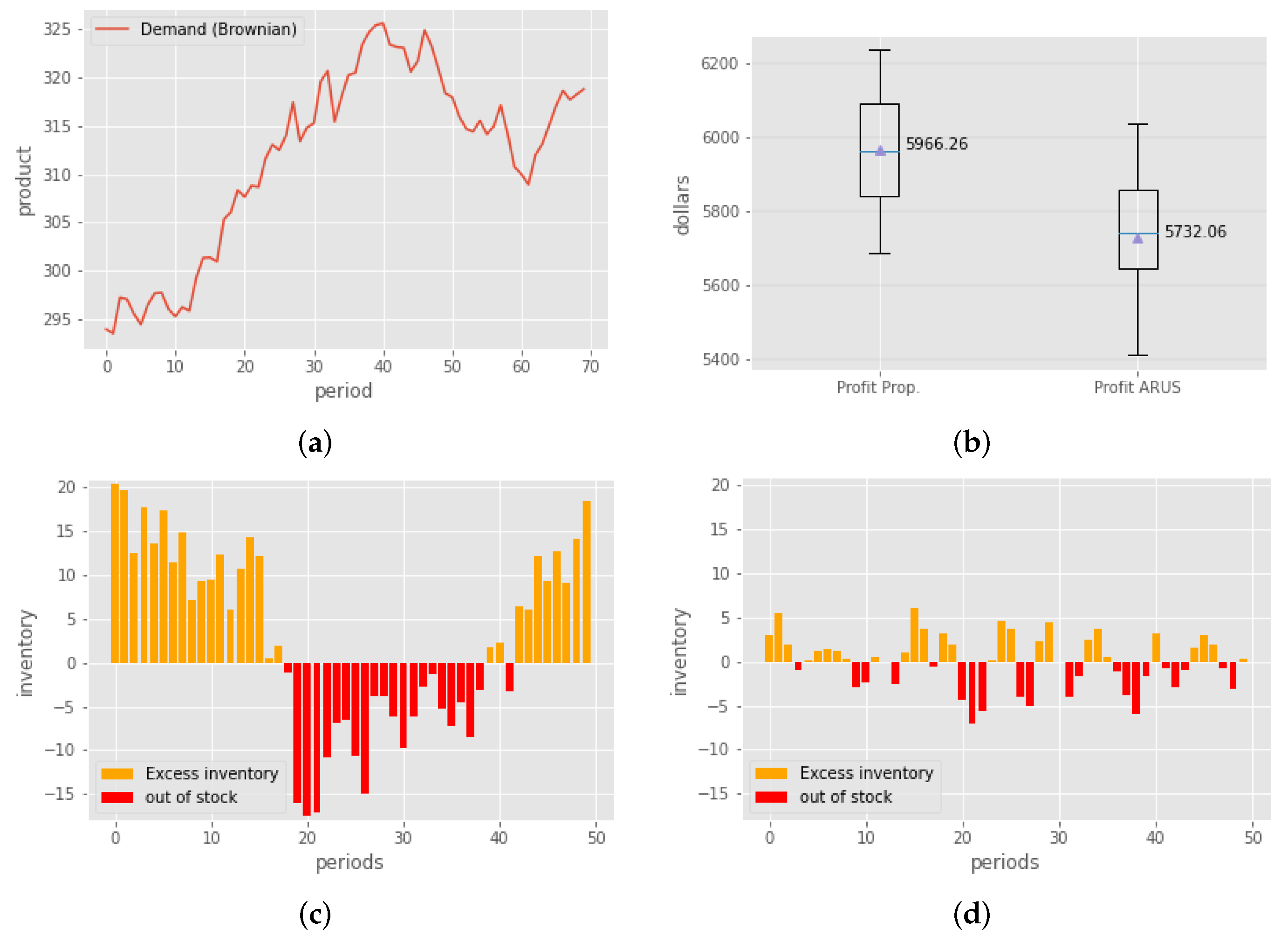
For the case where demand with Brownian movement was assumed, 150 periods were simulated. In Figure 3a, the behavior of the demand for periods 1–50 can be observed. Figure 3c,d show the behavior, with inventory estimates of ARUS and the proposed method. It should be noted that the ARUS process is not optimized for this type of process and only serves to illustrate the flexibility of the algorithm proposed for different types of demand. For this example, the proposed method outperformed the ARUS method by a wide margin.
5. Conclusions
In this work, we proposed a modification of the single-period inventory problem by introducing the GP to model the distribution of market demand. Historical demand data were adjusted by the GP, and the model was used to estimate the behavior of the demand.
In numerical examples used to evaluate the proposed method, we obtained fewer excess inventory units and shortage units with respect to the classic approach of modeling the distribution of demand as uniform. In a comparison between the ARUS and proposed model, when assuming demand as an AR process, it was observed that although the results in profit presented a difference of fewer than USD 300 between the two models, with a higher profit in the proposed one, the excess inventory was much greater in the ARUS method. This quantity is important since, depending on the demand behavior, with the ARUS model, there would be higher levels of inventory, which represents a significant amount of costs associated with its management. However, with the proposed model, low inventory levels were observed, and they were observed to oscillate between maximum quantities of 50 pieces. Therefore, it is concluded that the proposed model is better for establishing an inventory policy in the SPP, which means better prediction of the behavior of demand and therefore facilitating a better decision when buying the quantities of materials required to meet said demand. Its importance lies in the fact that this proposed method could be applied to a great diversity of products that depend on complex demand trends, e.g., the automotive sector, where car sales increase at the end of the year, affecting inventory needs of all materials required to assemble one. The companies could anticipate, with their suppliers, their purchase decisions based on the behavior of demand and save money from low levels of inventory. When demand is modeled as a Brownian motion process, it was once again observed that the results obtained in terms of profit saving with the proposed model were higher than with the ARUS method. Although these results pertain to a difference of fewer than USD 250, the inventory levels were also higher than in the proposed model. Finally, in the case in which the demand was modeled as an ARMA process, in the same way, lower levels of inventories were obtained, from which we concluded that by indistinctly modeling SPP demand with our model, we obtained better demand adjustment and low inventory quantities.
The benefits and industrial implications of the proposed method of establishing inventory levels include flexibility when monitoring the inventory control system due to better prediction, improvements in short- or medium-term projections, and consequently, reductions in inventories and costs associated with their storage. Because modeling demand accurately is a complicated task, in the industry, a common way to predict demand is to approximate order amount estimates using past demand. In this sense, having modeling alternatives that can estimate material requirements associated with inventory quantities would facilitate long-term decision-making in any company, particularly because it would anticipate changing events, therefore enabling rapid corrective action. Finally, we propose that better demand estimates could potentially be obtained if future work were to incorporate attributes of the complete supply- chain process other than demand information.
Author Contributions
All the authors contributed to the publishing of this article. All authors carefully studied the relevant literature on inventory models and GP estimation research. J.M. was mainly responsible for sorting out the overall thinking of the paper, writing the paper, and subsequent revisions. L.A.-S. was mainly responsible for the selection of the inventory model and cooperating with the writing. B.M. was responsible for paper’s mathematical design and inspection of the formulae. J.L.G.-A. provided technical guidance during the writing and revision of the paper. All authors have read and agreed to the published version of the manuscript.
Funding
This research received no external funding.
Institutional Review Board Statement
Not applicable.
Informed Consent Statement
Not applicable.
Data Availability Statement
Data are available upon request to the corresponding authors.
Conflicts of Interest
The authors declare no conflict of interest.
References
- Hadley, G.; Whitin, T.M. Analysis of Inventory Systems; Prentice-Hall: Englewood Cliffs, NJ, USA, 1963. [Google Scholar]
- Guo, M.; Chen, Y.W.; Wang, H.; Yang, J.B.; Zhang, K. The single-period (newsvendor) problem under interval grade uncertainties. Eur. J. Oper. Res. 2019, 273, 198–216. [Google Scholar] [CrossRef]
- Kitaeva, A.V.; Livshits, K.I.; Ulyanova, E.S. Estimating the Demand Parameters for Single Period Problem, Markov-modulated Poisson Demand, Large Lot Size, and Unobserved Lost Sales. IFAC-PapersOnLine 2018, 51, 882–887. [Google Scholar] [CrossRef]
- Kitaeva, A.V.; Stepanova, N.V.; Zhukovskaya, A.O.; Jakubowska, U.A. Demand estimation for fast moving items and unobservable lost sales. IFAC-PapersOnLine 2016, 49, 598–603. [Google Scholar] [CrossRef]
- Guo, Z.; Liu, Y. Modelling single-period inventory problem by distributionally robust fuzzy optimization method. J. Intell. Fuzzy Syst. 2018, 35, 1007–1019. [Google Scholar] [CrossRef]
- Qin, Z.; Kar, S. Single-period inventory problem under uncertain environment. Appl. Math. Comput. 2013, 219, 9630–9638. [Google Scholar] [CrossRef]
- Liu, B. Some research problems in uncertainty theory. J. Uncertain Syst. 2009, 3, 3–10. [Google Scholar]
- Chou, S.; Chen, C.W. Supply chain coordination: An inventory model for single-period utility product under fuzzy demand. Int. J. Adv. Manuf. Technol. 2017, 88, 585–594. [Google Scholar] [CrossRef]
- Ban, G.Y.; Rudin, C. The big data newsvendor: Practical insights from machine learning. Oper. Res. 2019, 67, 90–108. [Google Scholar] [CrossRef] [Green Version]
- Bastani, H.; Bayati, M. Online decision-making with high-dimensional covariates. Forthcom. Oper. Res. 2015, 68, 276–294. [Google Scholar] [CrossRef]
- Zhang, Y.; Gao, J. Assessing the performance of deep learning algorithms for newsvendor problem. In International Conference on Neural Information Processing; Springer: Cham, Switzerland, 2017; pp. 912–921. [Google Scholar]
- Huber, J.; Müller, S.; Fleischmann, M.; Stuckenschmidt, H. A data-driven newsvendor problem: From data to decision. Eur. J. Oper. Res. 2019, 278, 904–915. [Google Scholar] [CrossRef]
- Rasmussen, C.E. Gaussian processes in machine learning. In Summer School on Machine Learning; Springer: Berlin, Germany, 2003; pp. 63–71. [Google Scholar]
- Bodin, E.; Campbell, N.D.; Ek, C.H. Latent gaussian process regression. arXiv 2017, arXiv:1707.05534. [Google Scholar]
- Fox, E.; Dunson, D. Multiresolution gaussian processes. Adv. Neural Inf. Process. Syst. 2012, 25, 737–745. [Google Scholar]
- Taha, H.A. Operations Research An Introduction; CRC Press: Boca Raton, FL, USA, 2017. [Google Scholar]
- Rossi, R.; Prestwich, S.; Tarim, S.A.; Hnich, B. Confidence-based optimisation for the newsvendor problem under binomial, Poisson and exponential demand. Eur. J. Oper. Res. 2014, 239, 674–684. [Google Scholar] [CrossRef] [Green Version]
- Khouja, M. The single-period (news-vendor) problem: Literature review and suggestions for future research. Omega 1999, 27, 537–553. [Google Scholar] [CrossRef]
- Cristianini, N.; Shawe-Taylor, J. An Introduction to Support Vector Machines and Other Kernel-Based Learning Methods; Cambridge University Press: Cambridge, UK, 2000. [Google Scholar]
- Carrizosa, E.; Olivares-Nadal, A.V.; Ramírez-Cobo, P. Robust newsvendor problem with autoregressive demand. Comput. Oper. Res. 2016, 68, 123–133. [Google Scholar] [CrossRef]
- Petrović, D.; Petrović, R.; Vujošević, M. Fuzzy models for the newsboy problem. Int. J. Prod. Econ. 1996, 45, 435–441. [Google Scholar] [CrossRef]
- Zhang, X. Evolution of ARMA demand in supply chains. Manuf. Serv. Oper. Manag. 2004, 6, 195–198. [Google Scholar] [CrossRef]
- Gaur, V.; Giloni, A.; Seshadri, S. Information sharing in a supply chain under ARMA demand. Manag. Sci. 2005, 51, 961–969. [Google Scholar] [CrossRef] [Green Version]
- Pedregosa, F.; Varoquaux, G.; Gramfort, A.; Michel, V.; Thirion, B.; Grisel, O.; Blondel, M.; Prettenhofer, P.; Weiss, R.; Dubourg, V.; et al. Scikit-learn: Machine Learning in Python. J. Mach. Learn. Res. 2011, 12, 2825–2830. [Google Scholar]
- Abramowitz, M.; Stegun, I.A. Handbook of Mathematical Functions with Formulas, Graphs, and Mathematical Table; National Bureau of Standards Applied Mathematics Series 55; US Department of Commerce: Washington, DC, USA, 1965. [Google Scholar]
- Vickson, R.G. A single product cycling problem under Brownian motion demand. Manag. Sci. 1986, 32, 1336–1345. [Google Scholar] [CrossRef]
Figure 1.
(a) Optimal value of the order quantity over time, as determined by the models, (b) held units on inventory, as determined by the models, (c) shortage units as determined by the models, and (d) summary of the simulation; position of the arithmetic means are highlighted by a triangle.
Figure 1.
(a) Optimal value of the order quantity over time, as determined by the models, (b) held units on inventory, as determined by the models, (c) shortage units as determined by the models, and (d) summary of the simulation; position of the arithmetic means are highlighted by a triangle.

Figure 2.
(a) AR process as demand, (b) profit boxplot of ARUS and proposed method, (c) ARUS inventory, and (d) proposed method inventory.
Figure 2.
(a) AR process as demand, (b) profit boxplot of ARUS and proposed method, (c) ARUS inventory, and (d) proposed method inventory.

Figure 3.
(a) Brownian motion as demand, (b) profit box plot of ARUS and proposed method, (c) ARUS inventory, and (d) proposed method inventory.
Figure 3.
(a) Brownian motion as demand, (b) profit box plot of ARUS and proposed method, (c) ARUS inventory, and (d) proposed method inventory.


Table 1.
List of abbreviations.
| Abbreviation | Definition |
|---|---|
| AR | Autoregressive process |
| ARMA | Autoregressive moving-average |
| ARUS | Autoregressive process based on Uncertainty Sates |
| GP | Gaussian process |
| MA | Moving-average |
| NSM | Normal estimation method |
| SPP | single-period problem |
Publisher’s Note: MDPI stays neutral with regard to jurisdictional claims in published maps and institutional affiliations. |
© 2022 by the authors. Licensee MDPI, Basel, Switzerland. This article is an open access article distributed under the terms and conditions of the Creative Commons Attribution (CC BY) license (https://creativecommons.org/licenses/by/4.0/).
Share and Cite
MDPI and ACS Style
Mejia, J.; Avelar-Sosa, L.; Mederos, B.; García-Alcaraz, J.L. Inventory Model with Stochastic Demand Using Single-Period Inventory Model and Gaussian Process. Processes 2022, 10, 783. https://doi.org/10.3390/pr10040783
AMA Style
Mejia J, Avelar-Sosa L, Mederos B, García-Alcaraz JL. Inventory Model with Stochastic Demand Using Single-Period Inventory Model and Gaussian Process. Processes. 2022; 10(4):783. https://doi.org/10.3390/pr10040783
Chicago/Turabian StyleMejia, Jose, Liliana Avelar-Sosa, Boris Mederos, and Jorge L. García-Alcaraz. 2022. "Inventory Model with Stochastic Demand Using Single-Period Inventory Model and Gaussian Process" Processes 10, no. 4: 783. https://doi.org/10.3390/pr10040783
Note that from the first issue of 2016, this journal uses article numbers instead of page numbers. See further details here.