Mass and Magnetic Moment of the Electron and the Stability of QED—A Critical Review


Bogoljubov Labaratory of Theoretical Physics, Joint Institute for Nuclear Reseach, 141980 Dubna, Russia
*
Author to whom correspondence should be addressed.
Physics 2024, 6(1), 237-250; https://doi.org/10.3390/physics6010017
Submission received: 22 November 2023
/
Revised: 22 January 2024
/
Accepted: 26 January 2024
/
Published: 18 February 2024
(This article belongs to the Special Issue 75 Years of the Casimir Effect: Advances and Prospects)
Abstract
:The anomalous magnetic moment of the electron, first calculated by Schwinger, lowers the ground state energy of the electron in a weak magnetic field. It is a function of the field and changes signs for large fields, ensuring the stability of the ground state. This has been shown in the past 50 years in numerous papers. The corresponding corrections to the mass of the electron have also been investigated in strong fields using semiclassical methods. We critically review these developments and point out that the calculation for low-lying excited states raises questions. Also, we calculate the contribution from the tadpole diagram, the relevance of which was observed only quite recently.
1. Introduction
Quantum electrodynamics (QED) is the fundamental theory for describing the interaction of matter and light. On the classical level, these are the Maxwell theory and the relativistic mechanics, joined by a covariant coupling. QED is the quantum version of these. It was formulated quite early in the history of quantum mechanics, beginning with the paper of Paul Dirac. One of the first calculations of QED effects was the effective Lagrangian of Werner Heisenberg and Hans Euler [1], and the first new effect predicted using QED was the scattering of light on light. About ten years later, in 1948, Hendrick Casimir found [2] a vacuum interaction between neutral conducting plates caused by the quantized electromagnetic field confined between the plates. These two effects can be interpreted as loop correction, or radiative correction, to external influences. In the first case, such influence is provided by a classical electromagnetic field, and in the second case, it is provided by a conductor boundary condition on the plates (or by the freely movable charges within the plates), which also constitute a classical object.
It must be mentioned that there is a different interpretation for these effects saying that the vacuum of QED is filled with a fluctuating electromagnetic field, the interaction of which with the mentioned influences causes the effects. However, in a more formal approach, there is no need to speak about fluctuating fields. Namely, the mentioned effects can be equivalently described as vacuum-to-vacuum transition amplitude in an external field or as the vacuum expectation value of the energy–momentum tensor in the presence of external influences. For details, we refer to one of many books on this topic [3].
Beyond the two mentioned effects go the radiative, or loop, corrections like the anomalous magnetic moment of the electron and the Lamb shift. The former one can be viewed as a correction to the mass of the electron and to its magnetic moment, . The magnetic moment can be expressed as in terms of the Bohr magneton, , and the gyromagnetic ratio, g. From the Dirac equation, follows, whereas the radiative corrections cause a deviation, , called the anomaly of the magnetic moment. In 1948, Julian Schwinger found [4] in the lowest order in the fine structure constant, . This anomaly lowers the energy of the ground state of an electron in a magnetic field. Also, it results in a split of the excited energy levels. This split was measured in the so-called experiments with high precision and showed an excellent agreement with the theory (including higher powersof ).
In a weak magnetic field, the lowering of the ground state energy is proportional to the magnetic field. However, for an increasing field (as well as for higher excited states), it becomes a function of the field and it changes sign before the total energy can reach zero, ensuring the stability of the ground state. It must be mentioned that in theories with higher spin (), there is no stability. An example is quantum chromodynamics (QCD), where the so-called Savvidy vacuum is unstable, as shown in Ref. [5]; for a recent review, see [6].
In line with these examples, the Casimir effect is not only a phenomenon arising from vacuum fluctuations, but it may also bear instabilities under certain boundary conditions. In Appendix A, we refer to the Robin boundary conditions as an example. Like in a strong magnetic field, for certain values of the parameters, the energy of the lowest state may be below zero and constitute the instability of the system. It must be mentioned that in the literature on the Casimir effect, a situation with instabilities is rarely considered, although it well deserves more attention.
The present paper is a critical review on the question of the stability of QED in a magnetic field. The point is the following. While for the ground state the stability can be shown using a quite simple calculation and for high excited states and/or strong magnetic field using asymptotic methods, for lower exited states and medium fields, one is left with numerical investigation. Such analysis was performed in Ref. [7].
However, as we point out here, there are questions about the methods used in Ref. [7]. In addition, recently, in Ref. [8], it was observed that a class of diagrams (one-particle irreducible ones) do not vanish in distinction from earlier belief and may give an additional contribution.
For this reason, in what follows, we are interested only in the one-loop correction to the mass of the electron in a homogeneous magnetic field. Therefore, we do not consider the motion of the electron in the direction of the field and use the simplified notation.
It worth noting that the motion of an electron in a magnetic field is a field of vital interest, not so much in connection with the stability of QED as in connection with the synchrotron radiation which appears on the tree level as well as from the imaginary part of the radiative correction to the electron mass, see [9] and the book [10], for example. An essential tool is the semiclassical approximation, i.e., mass correction for high excited levels, see [11,12,13].
The paper is organized as follows. In Section 2, we reproduce and discuss the formulas known in the literature with a focus on the proper time representation. In Section 2.1 and Section 2.2, we discuss the problems which appear. In Section 3, we consider the one-particle irreducible (1PI) contribution. Section 4 gives conclusions of the study.
Throughout the paper, we use notations with for the reduced Planck’s constant, ℏ, and the speed of light, c.
2. The Mass and the Magnetic Moment of the Electron in a Magnetic Field
We consider the effective Dirac equation, i.e., the Dirac equation with loop corrections,
in one loop approximation. Here, x represents a four-dimensional coordinate, is the wave function, m denotes the mass of a particle. The covariant derivative is , with the Dirac matrices, , where e is the elementary charge, denotes the electromagnetic potential, the Greek indices take the values 0 (for the time coordinate), 1, 2, and 3 (space), and the self-energy operator, , reads
![Physics 06 00017 i001]() where the wavy line represents the photon propagator, , the doubled line represents dressed electron propagator and the dots represent interaction vertices. The spinor propagator , which is ‘exact’ in the field , obeys
where is the Dirac delta function.
where the wavy line represents the photon propagator, , the doubled line represents dressed electron propagator and the dots represent interaction vertices. The spinor propagator , which is ‘exact’ in the field , obeys
where is the Dirac delta function.

From Equation (1), for the electron, a mass,
follows with a mass correction . In the given order of approximation, is the expectation value of the self-energy operator in the unperturbed states.
From here on, we consider a homogeneous magnetic field, H. Then, the mass correction is the average
and it depends on the state of the electron. The eigenfunctions, taken in coordinate representation, read , and they obey the Dirac equation
The are the known eigenspinors, and the one-particle energy is
where is the momentum third space-component.
The states are numbered by N, and the spin projection is . The number N consists of two parts,
where numbers the Landau levels in the magnetic field. The ground state has and (spin projection parallel to the field). The excited states are doublets, which are degenerated on the tree level and split by the radiative correction.
As soon as , the mass correction (5) can be written in the form
for the excited states. For the ground state, one has only
A split like in the excited states is formally possible, but physically meaningless.
Making a non-relativistic approximation in (7), one comes to
For the free Dirac equation, follows, and from the loop correction, one has
where is the anomaly factor and is the so-called anomalous magnetic moment. Comparing Equation (11) with Equation (7), one identifies
This way, the anomaly factor becomes a function of both the field and the state.
For the calculation of the mass correction, there are two known methods. The first starts from the representation of the electron propagator in terms of the eigenspinors and the one-particle energies , which is an eigenfunction representation. This way was used in Refs. [14,15]. The representation of the mass correction is in terms of an integral over the photon loop momentum (in polar coordinates and ) and a sum over the intermediate states of the electron. It is convenient for strong fields since in that case only the lowest intermediate state contributes.
The second method uses the proper time representation of the propagators. In Ref. [16], the spinor propagator in the magnetic field was represented this way by performing the sum over the intermediate states. In Ref. [17], this representation was used to obtain an integral representation of the self-energy operator, .
In Ref. [18], a similar result was obtained using the algebraic procedure of Schwinger [19]. This method allows us to obtain the result through bypassing the summation of the eigenfunctions. The method was refined in a subsequent paper [20], and we follow the representation given there.
We use the following notations instead of the ones used in Ref. [20]. We change the integration variable . For the energy E, we insert (7), and set . In addition, we set (except in the factor in front) and also so that one has: , and . Finally, the prime is dropped: . With this notation, Equation (32) from Ref. [20] reads
where
is the ultraviolet subtraction and
Equation (25) from Ref. [20] defines as
and Equation (29) of Ref. [20] defines
which appears in the denominator.
Actually, these notations are not convenient enough. For that reason, we rewrite the notations. We start with the definition
Multiplying h by its complex conjugate, one can see see that factorizes,
Further, let us consider
which allows one to write
Next, let us consider in Equation (16). We write the trigonometric functions as sum/difference of the corresponding exponentials, and with Equation (22) one arrives at
where ‘c.c.’ denotes the complex conjugate. Using these formulas, we rewrite F in Equation (16) in the form
In this representation, the first two terms are interrelated by the complex conjugation and spin reversal: . The third term is of a real value.
The expression (24) can be simplified by keeping in the third term only the contributions from the ‘1’ in the numerator,
Finally, one arrives at
The expression (26) coincides with that in Ref. [17] with , up to an overall factor , of which Ref. [17] has more in the denominator (probably a typo).
In Ref. [7], the expression for was taken over from Ref. [17] (using different notations). Also using the operator method, in Ref. [21], a representation—Equation (3.18) in Ref. [21]—was derived which coincides with the above one. This representation was also taken over in Ref. [22], Equation (1), where, however, new notations were introduced, , for instance. Regrettably, the last term in the second line in Equation (1) [22] has a misprint and coincides with Equation (1) if one substitutes .
In Ref. [7], a further set of notations was introduced. In Equation (8), the energy correction is split into real and imaginary parts. This is the expression which in Ref. [7] was used for the numerical evaluation. It can be obtained from Equation (26) with the application of Equation (7), which here takes the form . Equation (26) then reads:
with
In order to investigate the structure of the expression F in Equation (14), it is necessary to look for the singularities in the complex plane. Denoting , let us first look for the zeros of the expression h (19),
For , one obtains two equations:
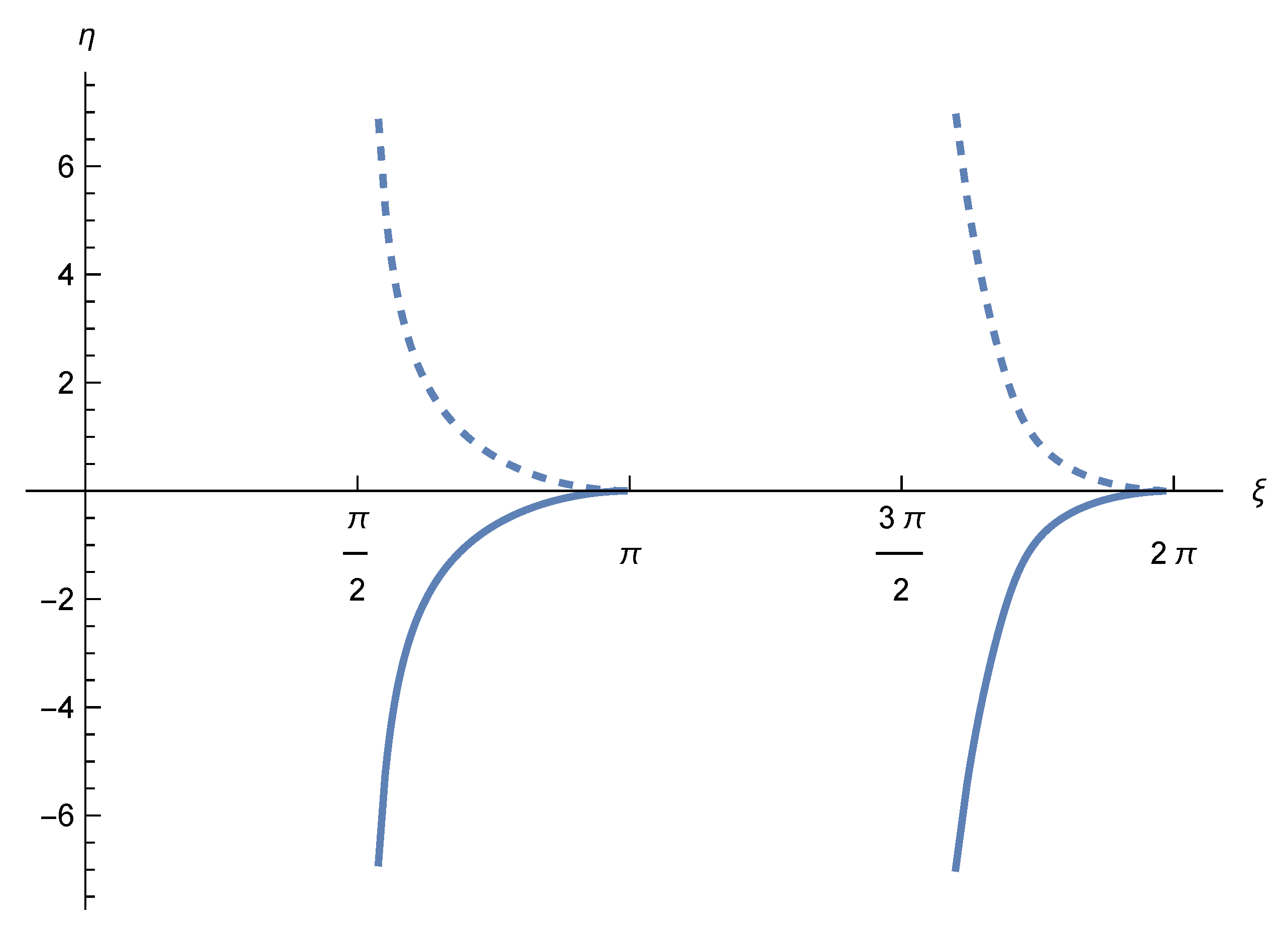
This way, the zeros of h are in the upper half-plane. Straightforwardly, has its zeros in the lower half-plane. For , these zeros reach the real axis in . For , the zeros go to infinity, , . The zeros are shown in Figure 1.
Since h has zeros only in the upper half-plane, according to the exponential factor in Equation (14), one may rotate the integration path towards the negative imaginary axis, . The result is a well-converging expression which allows for an immediate numerical evaluation. We repeat here in Figure 2 the representation given in Ref. [23].
For the excited states, the numerical evaluation is considerably more complicated. So far, only one attempt has been undertaken [7], which we consider in Section 2.1 just below.
2.1. On the Numerical Evaluation in Ref. [7] for the Excited States
In Section III of Ref. [7], it is mentioned that a numerical integration over the real x-axis is complicated because of the singularities in . A rotation of the integration path downwards in the complex plane, , would cross the singularities (see Figure 1). In Ref. [7], the authors use the following method. The u-integration is divided into two parts at some . For , there are no problems on the real axis and a numerical integration is possible. For , they turn the integration path towards the imaginary axis, see Equation (11) in Ref. [7]. However, this is not possible. As one can see in Figure 1, there are zeros in the denominator for all values of u. From this, we conclude that the numerical results in Ref. [7] are questionable.
2.2. On the Strong Field Limit
The limit of the strong magnetic field, , was calculated for the ground state in Refs. [18,24]. Recently, using an expression similar to Equation (35) from Ref. [23], the limit was recalculated, including the constant term,
where is the Euler’s constant.
For the low exited states (), there is only one calculation of the strong field limit [24]. It is in terms of the eigenfunction method and it is only for the spin-dependent part. It delivered
This way, for a strong field, the mass correction is also positive.
2.3. The Mass Correction for Low-Lying Excited States
An attempt to calculate this mass correction from the formulas which were reproduced in Section 2.2 above hits the following problem. When turning the integration path in (14) into the complex plane, , besides the contributions from the poles which one crosses, the following integral shows up:
However, for , one observes an asymptotic behavior, using Equations (19) and (30) with ,
where
was used. In addition, there is the factor in the integrand. This way, one observes an exponential growth in the integrand for for , i.e., for all finite H. Let us mention that this divergence is absent in the ground state, i.e., for . Also, this divergence cannot be related to the infrared divergence of the mass operator in Equation (2), since in Equation (5) is taken in states. Now, one could speculate on a cancellation from the pole contributions. But this is quite unlikely.
One may wonder how under such circumstances the weak-field expansion derived in Refs. [18,25,26] may be possible. The point is that for real x an expansion in the powers of u and x brings the power N down to factors N, and the resulting, oscillating integrals well may give finite answers. And they do, as follows from the mentioned papers. However, it is clear that the low-field expansion must be an asymptotic one.
3. The Contribution from the Tadpole Diagram
As observed quite recently in Ref. [8], 1PI diagrams can contribute to the effective Lagrangian in a homogeneous background field. The feature is that a tadpole diagram does not vanish. It contributes to the electron self-energy,
![Physics 06 00017 i002]()

The tadpole diagram can be derived from the one-loop Heisenberg–Euler (HE) Lagrangian (see, e.g., [27]) that
with . To mention is the possibility of deriving it from the worldline methods as performed, for example, in Ref. [28] for the spinor propagator. Such a diagram contributes a current (in Ref. [8] called a photon current),
where, for a constant purely magnetic field, B, directed along the z-axis, , , is the 4-momentum, is the antisymmetric Levi-Civita symbol, is the four-dimensional Dirac delta, with [8]
following. In Equation (43), the indices and take only values 1 and 2. In Equation (44), stands for the Hurwitz zeta function.
As it stands, the expression (44) is zero due to the factor k in front of the delta function and the general theory of distributions, and from symmetry reasons as well. However, a more detailed investigation [8] made a regularization of the delta function by considering a non-constant background field. The reason for the vanishing of Equation (43) is that a constant background field cannot support momentum transfer and therefore the momentum k must be zero. However, in a non-constant field, this argument cannot be applied and, in the limit of removing the regularization, one comes to an undefined expression of the type zero times infinity, to be considered in more details. The calculation realization rests on the ‘local constant field approximation’ [29], which allows us to use the expression of the one-loop effective Lagrangian for constant fields. This way, Ref. [8] calculated the 1PI contribution to the two-loop HE Lagrangian.
A similar effect appears also for the mass correction of the electron. From the Feynman rules and from Equation (41), a mass correction,
follows, which adds to in Equation (5).
In the sense of some regularization, we take for the delta function in Equation (43) the expression
which is most convenient in the given case. Then, the mass correction in Equation (45) can be calculated using the states ; these states are known, see, e.g., [30]. In order to be close to the notations of Ref. [30], we change the notation from N from Section 2 to n, and note
where the following notations, also close to those in Ref. [30], are used: , and
where is the radial variable, are the spinor factors for spin projection and enumerates the energy levels (7). These levels are degenerated with respect
to the orbital quantum number l, which is related by
to the principal quantum number and takes values The radial wave functions are given by
in terms of Laguerre polynomials. Below, we set the electron mass m = 1.
Using Equations (47)–(50), the calculation of the matrix elements becomes just a computing task. Since the dependence on the momentum in the direction of the magnetic field can be restored by a Lorentz transform, we restrict ourselves to . The mass correction reads
Using momentum representation for the current and the Euclidean propagator, one obtains:
With Equation (48), the spinor diagonal matrix elements turn into
These matrix elements (55) are independent of the spin projection and, thanks to this, cannot contribute to the anomalous magnetic moment. Further, there is no contribution to the ground state () and no contribution to a spin flip. As well, one can observe that the dependence on the azimuthal angle, , dropped out so that, from Equation (47), the conservation of angular momentum for non-diagonal matrix elements follows. Finally, one has to insert Equations (47) and (55) into Equation (45) and are left with a radial integration,
so that one arrives at
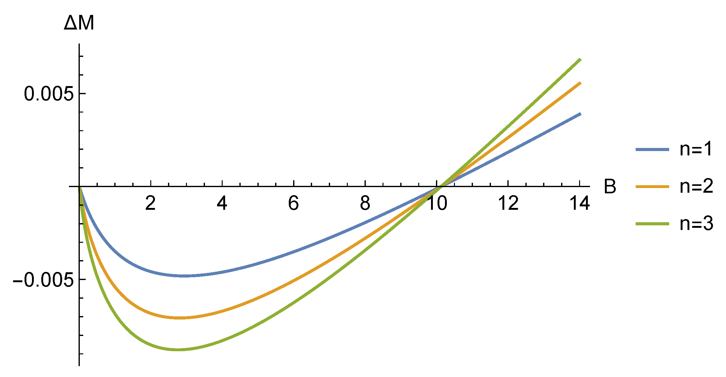
Here, is defined in Equation (44). As it turns out, this contribution to the mass corrections does not depend on the orbital momentum, l, similar to Equation (5). Examples for the dependence on the magnetic field are shown in Figure 3.
For the mass correction in a strong field, using the asymptotics of derived in Equation B.6 of Ref. [8] one obtains
This way, the contribution from the tadpole graph follows the general expectation, a negative contribution for small fields and a positive contribution for strong fields.
4. Conclusions
We reconsidered the calculation of the one-loop mass correction of the electron in a homogeneous magnetic field. There are two kind of representations known in the literature. One is in terms of eigenfunctions, and the other one uses the proper time representation and the operator method. We focused on the second case and compared the corresponding results obtained by different authors. In convenient notations, the result can be best written in the form in Equation (14), with W (26) (or (27)). Quite obvious misprints in the various papers are identified.
For studying the structure of the integrand F, Equation (26) is the most convenient since it has the simplest form of the denominators. On the real x-axis, one observes for , simple poles in , . The ratio in front is regular, and the last term in Equation (26) also has a simple pole if accounting for the integration over u and the factor () in the nominator. In the complex plane, one observes simple poles, the locations of which are shown in Figure 1.
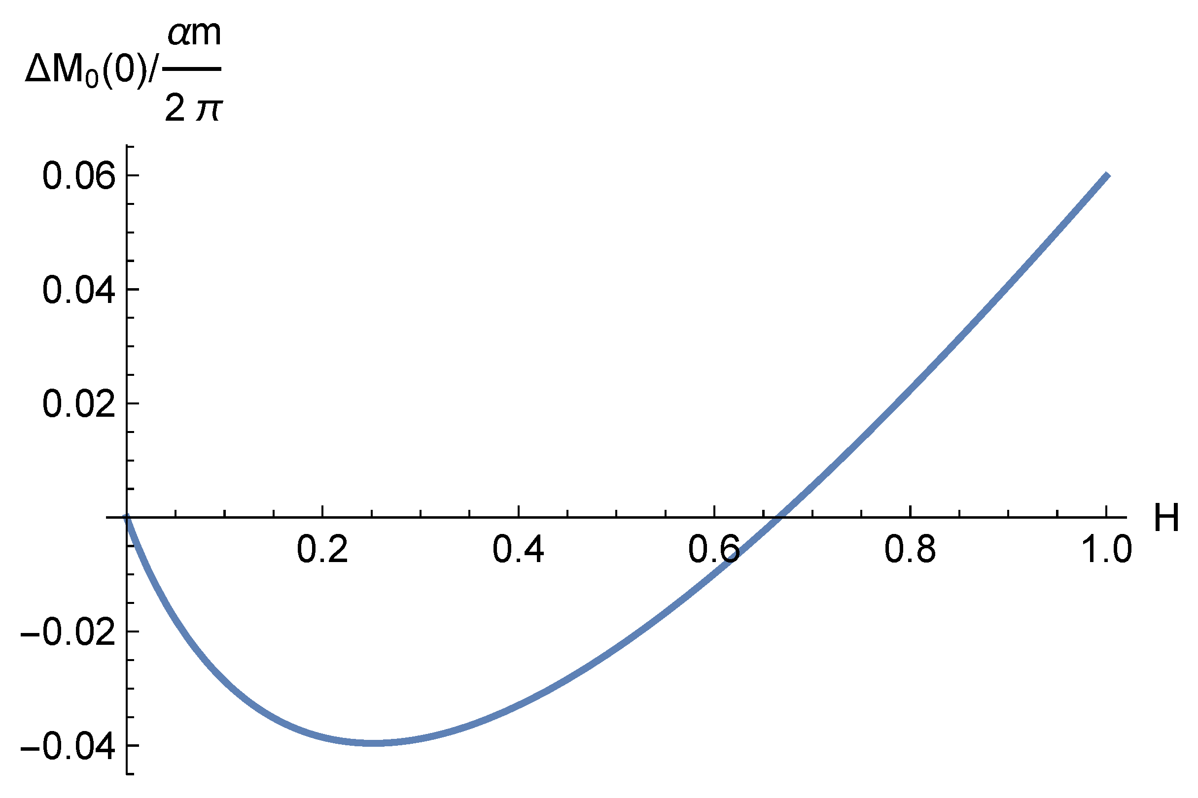
As for the ground state, there are coinciding results from all the studies referred to here. The mass correction is shown in Figure 2 and its asymptotics for are given in Equation (36). The finding demonstrates the stability of the ground state for arbitrary strength of the magnetic field.
For the low excited states, a similar result was obtained numerically in Ref. [7]. However, the method used for the calculation, as laid out in Section III in Ref. [7], raises questions as discussed in Section 2.1 here. More questions arise from the attempt to use the formulas shown in Section 2 for . As shown in Section 2.3, the rotation into the complex plane, , results in an exponential growth for , which should not have been there.
In addition, we calculated the so-far-overlooked contribution to the mass correction from the tadpole. The findings show no addition to the anomalous magnetic moment as well as no addition to the ground state energy. The tadpole contribution to the low excited states is shown in Figure 3. However, in order to compare this contribution with the contribution from Equation (2), more studies are necessary.
It worth mentioning that for high excited states, , which is of interest primarily for synchrotron radiation, a semiclassical approach delivers quite simple formulas which all demonstrate a growth in the mass correction in a magnetic field. We did not consider those calculations in the present paper.
In summary, the existing calculation for the mass correction of the electron in a magnetic field suggests no instability in QED. However, there are doubts in the correctness of the mentioned calculations, and a recalculation is advised.
Author Contributions
All authors contributed equally to this work. All authors have read and agreed to the published version of the manuscript.
Funding
This research received no external funding.
Data Availability Statement
Data is contained within the article.
Acknowledgments
The authors thank Sergey L. Lebedev for interesting discussions. The authors also thank the editors for English corrections.
Conflicts of Interest
The authors declare no conflicts of interest.
Appendix A. Robin Boundary Condition
In this Appendix, we refer to the basic formulas with the Robin boundary conditions, which are of interest in context with the Casimir effect and instabilities. The simplest case is a scalar field in four dimensions, obeying the wave equation and the boundary condition
where , the underlining in denotes a four-vector, is some parameter and we consider . After a Fourier transform in time and with the directions parallel to the plate,
the equation follows. With the ansatz , from the boundary condition (A1), follows. One must assume to obtain a normalizable solution and to arrive at
for the frequency. For , the frequency is real. This solution describes a surface mode (known, for example, on the surface of metals). However, for , the frequency becomes imaginary and there will be a solution exponentially increasing in time. This is the mentioned instability, which is typically excluded from investigating the Casimir effect. It is interesting to note the similarities between Equations (A3) and (11).
References
- Heisenberg, W.; Euler, H. Folgerungen aus der Diracschen Theorie des Positrons. Z. Phys. 1936, 98, 714–732, English translation: Consequences of Dirac’s theory of positrons. Available online: http://neo-classical-physics.info/electromagnetism.html (accessed on 24 January 2024). [CrossRef]
- Casimir, H.B.G. On the attraction between two perfectly conducting plates. Proc. Kon. Ned. Akad. Wetensch. 1948, 51, 793–795. Available online: https://dwc.knaw.nl/DL/publications/PU00018547.pdf (accessed on 24 January 2024).
- Bordag, M.; Klimchitskaya, G.L.; Mohideen, U.; Mostepanenko, V.M. Advances in the Casimir Effect; Oxford University Press: Oxford, UK, 2009. [Google Scholar] [CrossRef]
- Schwinger, J. On quantum-electrodynamics and the magnetic moment of the electron. Phys. Rev. 1948, 73, 416–417. [Google Scholar] [CrossRef]
- Nielsen, N.K.; Olesen, P. Unstable Yang-Mills field mode. Nucl. Phys. B 1978, 144, 376–396. [Google Scholar] [CrossRef]
- Savvidy, G. From Heisenberg-Euler Lagrangian to the discovery of chromomagnetic gluon condensation. Eur. Phys. J. C 2020, 80, 165. [Google Scholar] [CrossRef]
- Geprägs, R.; Riffert, H.; Herold, H.; Ruder, H.; Wunner, G. Electron self-energy in a homogeneous magnetic field. Phys. Rev. D 1994, 49, 5582–5589. [Google Scholar] [CrossRef]
- Gies, H.; Karbstein, F. An addendum to the Heisenberg-Euler effective action beyond one loop. J. High Energy Phys. 2017, 2017, 108. [Google Scholar] [CrossRef]
- Erber, T. High-energy electromagnetic conversion processes in intense magnetic fields. Rev. Mod. Phys. 1966, 38, 626–659. [Google Scholar] [CrossRef]
- Sokolov, A.A.; Ternov, I.M. Synchrotron Radiation; Akademie-Verlag GmbH/Pergamon Press Ltd.: Berlin/Braunschweig, Germany, 1968; Available online: https://archive.org/details/isbn_080129455 (accessed on 24 January 2024).
- Ternov, I.; Tumanov, W. On question of the movement of polarized electrons in magnetic field. Izv. VUZov SSSR Ser. Fiz. [Bull. High Educ. Establ. USSR Ser. Phys.] 1960, 1, 155. (In Russian) [Google Scholar]
- Nikishov, A.I.; Ritus, V.I. Interaction of electrons and photons with a very strong electromagnetic field. Sov. Phys. Uspekhi 1970, 13, 303–305. [Google Scholar] [CrossRef]
- Baier, V.N.; Katkov, V.M.; Fadin, V.S. Radiation from Relativistic Electrons; Atomizdat: Moscow, Russia, 1973. (In Russian) [Google Scholar]
- Ternov, I.M.; Bagrov, V.G.; Bordovitsyn, V.A.; Dorofeev, O.F. Vacuum magnetic moment of an electron moving in a uniform magnetic field. Sov. Phys. J. 1968, 11, 11–16. [Google Scholar] [CrossRef]
- Kobayashi, M.; Sakamoto, M. Radiative-corrections in a strong magnetic-field. Prog. Theor. Phys. 1983, 70, 1375–1384. [Google Scholar] [CrossRef]
- Géhéniau, J.; Demeur, M. Solutions singulières des équations de Dirac, tenant compte d’un champ magnétique extérieur. Physica 1951, 17, 71–75. [Google Scholar] [CrossRef]
- Constantinescu, D.H. Electron self-energy in a magnetic field. Nucl. Phys. B 1972, 44, 288–300. [Google Scholar] [CrossRef]
- Tsai, W.-Y.; Yildiz, A. Motion of an electron in a homogeneous magnetic-field—Modified propagation function and synchrotron radiation. Phys. Rev. D 1973, 8, 3446–3460. [Google Scholar] [CrossRef]
- Schwinger, J. Classical radiation of accelerated electrons. II. A quantum viewpoint. Phys. Rev. D 1973, 7, 1696–1701. [Google Scholar] [CrossRef]
- Tsai, W.-Y. Modified electron propagation function in strong magnetic fields. Phys. Rev. D 1974, 10, 1342–1345. [Google Scholar] [CrossRef]
- Baǐer, V.N.; Katkov, V.M.; Strakhovenko, V.M. Operator approach to quantum electrodynamics in an external field: The mass operator. Sov. Phys. JETP 1975, 40, 225–232. Available online: http://jetp.ras.ru/cgi-bin/e/index/e/40/2/p225?a=list (accessed on 24 January 2024).
- Baǐer, V.N.; Katkov, V.M.; Strakhovenko, V.M. Structure of the electron mass operator in a homogeneous magnetic field close to the critical strength. Sov. Phys. JETP 1990, 71, 657–666. Available online: http://jetp.ras.ru/cgi-bin/e/index/e/71/4/p657?a=list (accessed on 24 January 2024).
- Bordag, M. On instabilities caused by magnetic background fields. Symmetry 2023, 15, 1137. [Google Scholar] [CrossRef]
- Ternov, I.M.; Bagrov, V.G.; Bordovitsyn, V.A.; Dorofeev, O.F. Concerning the anomalous magnetic moment of the electron. Sov. Phys. JETP 1969, 28, 1206–1209. Available online: http://jetp.ras.ru/cgi-bin/e/index/e/28/6/p1206?a=list (accessed on 24 January 2024).
- Newton, R.G. Radiative effects in a constant field. Phys. Rev. 1954, 96, 523–528. [Google Scholar] [CrossRef]
- Consoli, M.; Preparata, G. On the stability of the perturbative ground state in non-abelian Yang-Mills theories. Phys. Lett. B 1985, 154, 411–417. [Google Scholar] [CrossRef]
- Dunne, G.V. Heisenberg-Euler effective lagrangians: Basics and extensions. In From Fields to Strings: Circumnavigating Theoretical Physics; Shifman, M., Vainstein, A., Wheater, J., Eds.; World Scientific: Singapore, 2005; pp. 445–522. [Google Scholar] [CrossRef]
- Ahmadiniaz, N.; Bastianelli, F.; Corradini, O.; Edwards, J.P.; Schubert, C. One-particle reducible contribution to the one-loop spinor propagator in a constant field. Nucl. Phys. B 2017, 924, 377–386. [Google Scholar] [CrossRef]
- Karbstein, F.; Shaisultanov, R. Stimulated photon emission from the vacuum. Phys. Rev. D 2015, 91, 113002. [Google Scholar] [CrossRef]
- Sokolov, A.A.; Ternov, I.M. Radiation from Relativistic Electrons; American Institute of Physics Translation Series; American Institute of Physics: New York, NY, USA, 1986; Available online: https://archive.org/details/radiationfromrel0000soko/ (accessed on 24 January 2024).
Figure 1.
In the complex plane, , the locations of the zeros of h (19) (upper half-plane, dashed) and of (lower half-plane). In these curves, the parameter u takes values from at to at .
Figure 1.
In the complex plane, , the locations of the zeros of h (19) (upper half-plane, dashed) and of (lower half-plane). In these curves, the parameter u takes values from at to at .

Figure 2.
The mass correction , see Equation (10), for the ground state, divided by , as a function of the magnetic field. In the minimum, this function takes small values and must be additionally multiplied by to compare with the rest mass.
Figure 2.
The mass correction , see Equation (10), for the ground state, divided by , as a function of the magnetic field. In the minimum, this function takes small values and must be additionally multiplied by to compare with the rest mass.

Figure 3.
The mass correction in Equation (57), as a function of the magnetic field, B, for a few n values as indicated.
Figure 3.
The mass correction in Equation (57), as a function of the magnetic field, B, for a few n values as indicated.

Disclaimer/Publisher’s Note: The statements, opinions and data contained in all publications are solely those of the individual author(s) and contributor(s) and not of MDPI and/or the editor(s). MDPI and/or the editor(s) disclaim responsibility for any injury to people or property resulting from any ideas, methods, instructions or products referred to in the content. |
© 2024 by the authors. Licensee MDPI, Basel, Switzerland. This article is an open access article distributed under the terms and conditions of the Creative Commons Attribution (CC BY) license (https://creativecommons.org/licenses/by/4.0/).
Share and Cite
MDPI and ACS Style
Bordag, M.; Pirozhenko, I.G. Mass and Magnetic Moment of the Electron and the Stability of QED—A Critical Review. Physics 2024, 6, 237-250. https://doi.org/10.3390/physics6010017
AMA Style
Bordag M, Pirozhenko IG. Mass and Magnetic Moment of the Electron and the Stability of QED—A Critical Review. Physics. 2024; 6(1):237-250. https://doi.org/10.3390/physics6010017
Chicago/Turabian StyleBordag, Michael, and Irina G. Pirozhenko. 2024. "Mass and Magnetic Moment of the Electron and the Stability of QED—A Critical Review" Physics 6, no. 1: 237-250. https://doi.org/10.3390/physics6010017