New Insights into the Lamb Shift: The Spectral Density of the Shift

Abstract

In an atom, the interaction of a bound electron with the vacuum fluctuations of the electromagnetic field leads to complex shifts in the energy levels of the electron, with the real part of the shift corresponding to a shift in the energy level and the imaginary part to the width of the energy level. The most celebrated radiative shift is the Lamb shift between the $2s_{1/2}$ and the $2p_{1/2}$ levels of the hydrogen atom. The measurement of this shift in 1947 by Willis Lamb Jr. proved that the prediction by Dirac theory that the energy levels were degenerate was incorrect. Hans Bethe’s non-relativistic calculation of the shift using second-order perturbation theory demonstrated the renormalization process required to deal with the divergences plaguing the existing theories and led to the understanding that it was essential for theory to include interactions with the zero-point quantum vacuum field. This was the birth of modern quantum electrodynamics (QED). Numerous calculations of the Lamb shift followed including relativistic and covariant calculations, all of which contain a nonrelativistic contribution equal to that computed by Bethe. The semi-quantitative models for the radiative shift of Welton and Power, which were developed in an effort to demonstrate physical mechanisms by which vacuum fluctuations lead to the shift, are also considered here. This paper describes a calculation of the shift using a group theoretical approach which gives the shift as an integral over frequency of a function, which is called the “spectral density of the shift.“ The energy shift computed by group theory is equivalent to that derived by Bethe yet, unlike in other calculations of the non-relativistic radiative shift, no sum over a complete set of states is required. The spectral density, which is obtained by a relatively simple computation, reveals how different frequencies of vacuum fluctuations contribute to the total energy shift. The analysis shows, for example, that half the radiative shift for the ground state 1S level in H comes from virtual photon energies below 9700 eV, and that the expressions of Power and Welton have the correct high-frequency behavior, but not the correct low-frequency behavior, although they do give approximately the correct value for the total shift.

1. Introduction

In astronomy, in quantum theory, and in quantum electrodynamics (QED), there have been periods of great progress in which solutions to challenging problems have been obtained, and the fields have moved forward. However, in some cases getting the right answers can still leave fundamental questions unanswered. The Big Bang explained the origin of cosmic background radiation but left the problem of why the universe appears to be made of matter and not equal amounts of matter and antimatter [1]. In quantum theory, physicists can compute the behavior of atoms yet cannot describe a measurement in a self-consistent way [2], or make sense of the collapse of a photon wavefunction from a near infinite volume to a point [3]. In quantum electrodynamics, we can compute the Lamb shift of the H atom to 15 decimal places [4], yet we are left with the paradox of using perturbation theory to remove infinite terms or to understand a quantum vacuum with infinite energy. In this paper, several different approaches to the computation of the non-relativistic Lamb shift are examined. For these approaches, the Lamb shift can be expressed in different ways as an integral over the frequency of a spectral density. This paper analyzes of the differences in the non-relativistic spectral densities for the different approaches as a function of frequency and compares the spectral densities to those obtained using a group theoretical analysis. The integral of the spectral density over all frequencies gives the corresponding value of the non-relativistic Lamb shift.

Feynman called the three-page long 1947 non-relativistic Lamb shift calculation by Hans Bethe the most important calculation in quantum electrodynamics because it tamed the infinities plaguing earlier attempts [5,6]. When the sum over all states is evaluated numerically, it gives a finite prediction that agreed with experiment [7,8]. Dirac said it “fundamentally changed the nature of theoretical physics” [6]. Quoting the classic text of Quantum Electrodynamics, Volume 4 in the Landau and Lifshiftz series on Theoretical Physics: “This work provided the initial stimulus for the whole subsequent development of quantum electrodynamics” [5]. Yet when this calculation is explored more deeply, questions arise about it and about other fundamentally different calculations of the Lamb shift, for example, those by Welton [9] and Power [10], that employ different conceptual approaches that have similar high-frequency but different low-frequency behavior from Bethe’s result yet give approximately the same value for the level shift [6]. These three approaches to the Lamb shift and the corresponding vacuum energy densities have also been considered in [11].

There is an intimate relationship between radiative shifts and vacuum fluctuations. The shift can be interpreted as arising from virtual transitions induced by the quantum fluctuations of the electromagnetic field. Since the vacuum field contains all frequencies, virtual transitions to all states, bound and scattering, are possible. These short-lived virtual transition result in a slight shift in the average energy of the atom, a shift which is the Lamb shift [12]. The Lamb shift can also be described as an interaction of the electron with its own radiation field, yielding the same results as the vacuum field [6].

Shortly after Bethe’s calculation, Dyson published, as a problem assigned by Bethe, a calculation of the Lamb shift for a spinless electron [13]. Formal and rigorous relativistic perturbation theory calculations to first-order in the radiation field and to fourth order in the ratio of the velocity of the atomic electron to the velocity of light, based on the Dirac equation, including spin and relativistic effects, were carried out independently in 1949 by J. French and V. Weisskopf [14] and N. Kroll and W. Lamb [15]. They used a high-frequency cutoff for the non-relativistic contribution which also acted as a low-frequency cutoff for the relativistic portion, and when both contributions were added together, the sum was independent of the cutoff, and equaled a term corresponding to the Bethe log plus constants corresponding to relativistic corrections. Although these calculations were difficult and cumbersome, they have stood the test of time [16]. These relativistic calculations gave a value of 1052 MHz for the Lamb shift, compared to Bethe’s result of 1040 MHz, about a 1% difference. The determination of the second-order corrections for the Lamb shift is quite complicated. The most complete tabulation and systematic derivation was carried out by Erickson and Yennie [17]. Today the Lamb shift is computed precisely to over 10 decimal places to be about 1057 MHz, the largest error being due to the uncertainty in the radius of the proton [4].

At about the same time as the first relativistic calculations were published, Schwinger published a general covariant approach to quantum electrodynamics which he applied to the Lamb shift computation [18]. Within a year, three different approaches to quantum electrodynamics were independently developed that were relativistic and could deal with divergences with some success. Schwinger, Tomonaga, and Feynman each had proposed a manifestly covariant method, and shown its capability to address a broader range of QED problems than just the energy levels of the H atom [19]. Freeman Dyson showed that these three methods had essential similarities and were mutually consistent [20].

The classic text, Quantum Electrodynamics, Volume 4 of the Landau and Lifshitz series on Theoretical Physics, second edition published in 1979, does the Lamb shift calculation by dividing the vacuum energy spectrum into a low and high-frequency region with a cutoff [5]. For the high-energy region, they use scattering theory based on Schwinger’s approach. For the low-frequency region they use non-relativistic kinematics and start with the expression for dipole radiation, which they transform with some mathematical operations on delta function; then they integrate over frequency and obtain essentially the same result as Bethe plus constants corresponding to vacuum polarization and other corrections that are not considered here. When the high and low-frequency results are added, the cutoff cancels. The final result contains the Bethe log. A slightly different approach is taken but with similar results in [21]. Another important text, published in 1980 by Itzykson and Zuber, starts with a modified Dirac equation with a fictitious photon mass, and that includes vacuum polarization and vertex corrections for an electron in a slowly varying external field [22]. This equation yields a level shift with two terms that correspond to the high-energy region and low-energy region. After evaluation, the sum of the terms is taken, the fictitious mass cancels, and the result is the Bethe log and a constant.

Modern QED texts use similar approaches. Weinberg uses a fictitious photon mass in the photon propagator which leads to a high and low-energy term [16]. When added, the fictitious mass cancels, yielding a constant and the Bethe log term. The evolution of Lamb shift calculations is outlined in [12] and the detailed status is in [23].

For the purposes of the present paper, which is a non-relativistic calculation of the radiative Lamb shift, not including vacuum polarization, it is important to note that Bethe’s non-relativistic result and the numerically evaluated Bethe log have been obtained in virtually all Lamb shift calculations, including all relativistic calculations [5,6,16,22]. The Bethe log represents the non-relativistic radiative contribution in all these diverse calculations. The Lamb shift spectral density obtained here can be integrated to obtain the non-relativistic Lamb shift, a quantity given by the Bethe logarithm. Furthermore, the integral can be taken to the desired energy to be consistent with a particular relativistic calculation. Thus, the spectral density computed is a standalone fundamental quantity that relates to all Lamb shift calculations described in the literature. Consequently, there is no need to consider the numerous relativistic calculations further in this paper.

Bethe’s non-relativistic calculation to order $\alpha$ in the vacuum field (one virtual photon) was based on second-order perturbation theory applied to the minimal coupling of the atom with the vacuum field, $(e/mc)\mathbf{A}·\mathbf{p}$, and a dipole approximation; here m, e, and $\mathbf{p}$ are the mass, charge and momentum of the electron, respectively, c is the speed of light in a vacuum, and $\mathbf{A}$ is the vector potential. This interaction leads to the emission and absorption of virtual photons corresponding to virtual transitions. The shift is expressed as a sum over the infinite number of intermediate states, bound and scattering, reached by virtual transitions. The predicted shift is divergent, but Bethe subtracted the term that corresponded to the linearly divergent vacuum energy shift for a free bare electron, essentially doing a mass renormalization to remove this higher-order divergence in the spectral density for the shift. For S states, the resulting spectral density has a 1/frequency behavior for frequencies above about 1000 eV/ℏ, (with ℏ the reduced Planck’s constant) giving a logarithmic divergence in the shift. Bethe used a high-frequency cutoff of $\omega =m{c}^2/\hslash$.

The models of Welton and Power embody different perspectives on the role of vacuum fluctuations than the Bethe calculation. Itzykson and Zuber note: “Charged particles interact with the fluctuations of the quantized electromagnetic field…we may give, following Welton, a qualitative description of the main effect: the Lamb shift” [22]. Welton’s semi-quantitative model for computing the Lamb shift was based on the perturbation of the motion of a bound electron in the H atom due to the quantum vacuum fluctuations altering the location of the electron, which resulted in a slight shift of the bound state energy [6,9,12]. This simplified intuitive model predicts a spectral density proportional to 1/frequency for all frequencies and a shift only for S states. The approach of Feynman [24], interpreted by Power [10], considers a large box containing H atoms and is based on the shift in the energy in the quantum vacuum field due to the change in the index of refraction arising from the presence of H atoms. This approach predicts that the shift in the energy in the vacuum field around the H atoms exactly equals the radiative shift [6,11]. It gives a spectral density with the same high-frequency dependence as Bethe, but a different low-frequency dependence. A similar calculation to Power’s models the Lamb shift as a Stark shift [6].

The Lamb shift has been previously computed using O(4) symmetry [25] and by using SO(4,2) symmetry [26] using a different approach from that presented here. In both these cases, the Bethe log is obtained for low-lying states as a converging series. The results presented here describe a calculation of the Lamb shift for all states that is based on a SO(4,2) group theoretical analysis of the H atom that allows us to determine the dependence of the shift on the frequency with no sum over states [27]. The spectral shift due to all virtual transitions is computed analytically.

The degeneracy group of the non-relativistic H atom is O(4), with generators angular momentum operator $\mathit{L}$ and Runge-Lenz vector $\mathit{A}$. A representation of O(4) of dimension $n^2$ exists for each value of the principal quantum number n, where the angular momentum L has values from 0 to $n-1$, and there are $2L+1$ possible values of $L_z=m$, the azimuthal quantum number. If this group is extended by adding a 4-vector of generators the non-invariance group SO(4,1) results, which has representations that include all states of different n and L and operators that connect states with different principal quantum numbers. Adding a 5-vector of additional generators produces the group SO(4,2) and allows us to express Schrödinger’s equation in terms of the new generators, and to make effective group theoretical calculations [27]. The basis states used permit both bound and scattering states to be included seamlessly [28] and no sum over states appears in the final expression for the spectral density. One advantage of this approach is that for each energy level it is possible to readily compute a spectral density for the shift whose integral over frequency from 0 to $m{c}^2/2\pi \hslash$ is the radiative shift that includes transitions to all possible states. This reveals how different frequencies of the vacuum field contribute to the radiative shift.

In this paper, the different results of Bethe, Welton and Power are compared to the group theoretical spectral density for the non-relativistic Lamb shift for the 1S ground state, and the 2S and 2P levels. With this new picture of the Lamb shift, differences between the various approaches are seen. Knowing the spectral density of the shift provides new insights into understanding the Lamb shift.

2. Background of Radiative Shift Calculations

The first calculation of the Lamb shift of a hydrogen atom was carried out by Bethe in 1947 [8], who assumed the shift was due to the interaction of the atom with the vacuum field. He calculated the shift using second-order perturbation theory, assuming that there was minimal coupling in the Hamiltonian

$$H_{\mathrm{int}}=-\frac{e}{mc}\mathbf{A}·\mathbf{p}+\frac{e^2}{2m{c}^2}{\mathbf{A}}^2,$$

(1)

where $\mathbf{A}$ is the vector potential in the dipole approximation for the vacuum field in a large quantization volume V:

$$\mathbf{A}=\sum _{\mathbf{k},\lambda }{\left(\frac{2\pi \hslash }{{\omega }_{k}V}\right)}^{1/2}(a_{\mathbf{k},\lambda }+a_{\mathbf{k},\lambda }^{†}){\mathbf{e}}_{\mathbf{k}\lambda },$$

(2)

where the sum is over the virtual photon frequency ${\omega }_k$, and the polarization $\lambda$; $a_{\mathbf{k},\lambda }$ and $a_{\mathbf{k},\lambda }^{†}$ are the annihilation and creation operators, and ${\mathbf{e}}_{\mathbf{k}\lambda }$ is a unit vector in the direction of polarization of the electric field. The shift from the ${\mathbf{A}}^2$ term is independent of the state of the atom and is therefore neglected. The total shift $\mathsf{\Delta }{E}_{n\mathrm{Tot}}$ for energy level n of the atom in state $|n\rangle$ is given by second-order perturbation theory as

$$\mathsf{\Delta }{E}_{n\mathrm{Tot}}=-\frac{2}{3{\pi }^2}\frac{\alpha }{m^2{c}^2}\sum _m{\left|{\mathbf{p}}_{mn}\right|}^2\int \frac{EdE}{E_m-E_n+E},$$

(3)

where the quantum vacuum field energy is $E=\hslash \omega$ and the momentum matrix elements are $|{\mathbf{p}}_{mn}|=|\langle m\left|\mathbf{p}\right|n\rangle |$. The sum is over all intermediate states $|m\rangle$, scattering and bound, where $m\ne n$ and the integral is over the energy E of the vacuum field. The fine structure constant is $\alpha =e^2/\hslash c$.

The integrand in Equation (3) has a linear divergence. Bethe observed that this divergence corresponded to the integral that occurs when the binding energy vanishes so $(E_m-E_n)\to 0$ and the electrons are free:

$$\mathsf{\Delta }{E}_{\mathrm{free}}=-\frac{2}{3{\pi }^2}\frac{\alpha }{m^2{c}^2}\sum _m{\left|{\mathbf{p}}_{mn}\right|}^2\int dE.$$

(4)

He subtracted this divergent term $\mathsf{\Delta }{E}_{\mathrm{free}}$ from the total shift $\mathsf{\Delta }{E}_{n\mathrm{Tot}}$,

$$\mathsf{\Delta }{E}_{nL}=\mathsf{\Delta }{E}_{n\mathrm{Tot}}-\mathsf{\Delta }{E}_{\mathrm{free}},$$

(5)

to obtain a finite observable shift $\mathsf{\Delta }{E}_{nL}$ for the state $|nL\rangle$:

$$\mathsf{\Delta }{E}_{nL}=\frac{2\alpha }{3\pi {\left(mc\right)}^2}\sum _m^s{\left|{\mathbf{p}}_{mn}\right|}^2{\int }_0^{\hslash {\omega }_c}dE\frac{(E_m-E_n)}{E_m-E_n+E-iϵ},$$

(6)

where ${\omega }_C$ is a cutoff frequency for the integration that Bethe took as $\hslash {\omega }_c=m{c}^2$. Using an idea from Kramers [6,29], Bethe did this renormalization, taking the difference between the terms with a potential present and without a potential present, essentially performing the free electron mass renormalization. He reasoned that relativistic retardation could be neglected and the radiative shift could be reasonably approximated using a non-relativistic approach and he cut the integration off at an energy corresponding to the mass of the electron. He obtained a finite result that required a numerical calculation over all states, bound and scattering, that gave good agreement with measurements [7,8,30].

The spectral density in the Bethe formalism, which is analysed in this paper, is the quantity in Equation (6) being integrated over E. It includes the sum over states m and the constants. The term for m represents the contribution to the Lamb shift for the virtual transition from state n to state m. Note that since the ground state is the lowest state, all intermediate states have higher energies so the ground state shift has to be positive.

For the purposes of comparison to the other calculations of the Lamb shift, it is helpful to show the next steps Bethe took to evaluate the shift $\mathsf{\Delta }{E}_n$ for S states, which have the largest shifts. Note that the spectral density in Equation (6) that will be analyzed is not affected by the subsequent approximations Bethe made to evaluate the integral. First, the $E-$ integration is carried out:

$$\mathsf{\Delta }{E}_n^{\mathrm{Bethe}}=\frac{2\alpha }{3\pi }{\left(\frac{1}{mc}\right)}^2\sum _m{\left|{\mathbf{p}}_{nm}\right|}^2(E_m-E_n)ln\frac{(m{c}^2+E_m-E_n)}{|E_m-E_n|}.$$

(7)

To simplify the evaluation Bethe assumed $|E_m-E_n|\ll m{c}^2$ in the logarithm and that the logarithm would vary slowly with the index m so it could be replaced by an average value,

$${\widehat{\mathsf{\Delta }E}}_n^{\mathrm{Bethe}}=\frac{2\alpha }{3\pi }{\left(\frac{1}{mc}\right)}^{2}ln\frac{m{c}^2}{|E_m-E_n{|}_{\mathrm{ave}}}\sum _m{\left|{\mathbf{p}}_{nm}\right|}^2(E_m-E_n),$$

(8)

where the hat over the $\mathsf{\Delta }E$ indicates this is an approximation to Equation (7). Now that the E-integration is done, the spectral density is no longer manifest. The summation can be evaluated using the dipole sum rule:

$$2\sum _m^s{\left|{\mathbf{p}}_{nm}\right|}^2\left(E_m-E_n\right)={\hslash }^2〈n\left|{\nabla }^{2}V\right|n〉.$$

(9)

where $\langle \dots \rangle$ indicates an expectation value. The Laplacian with a Coulomb potential $V=-Z{e}^2/r$ is ${\nabla }^{2}V\left(r\right)=4\pi Z{e}^2\delta \left(\mathbf{r}\right)$ which gives

$$〈n\left|{\nabla }^{2}V\right|n〉=4\pi Z{e}^2{\left|{\psi }_n\left(0\right)\right|}^2,$$

(10)

where Z is the positive charge of the nucleus, $\psi \left(r\right)$ is the wave function for the Coulomb potential and $|{\psi }_n{\left(0\right)|}^2$ is zero except for S states,

$${|{\psi }_n\left(0\right)|}^2=\frac{1}{\pi }{\left(\frac{Z\alpha mc}{n\hslash }\right)}^3.$$

(11)

For S states, this gives an energy shift equal to [6]

$${\widehat{\mathsf{\Delta }E}}_n^{\mathrm{Bethe}}=\frac{4m{c}^2}{3\pi }\alpha {\left(Z\alpha \right)}^4\frac{1}{n^3}ln\frac{m{c}^2}{|E_m-E_n{|}_{\mathrm{ave}}}.$$

(12)

The so-called “Bethe log” for an S state with principal quantum number n is

$$ln\frac{m{c}^2}{|E_m-E_n{|}_{\mathrm{ave}}}=\frac{{\sum }_m{\left|{\mathbf{p}}_{nm}\right|}^2(E_m-E_n)ln\frac{m{c}^2}{|E_m-E_n|}}{{\sum }_m{\left|{\mathbf{p}}_{nm}\right|}^2\left(E_m-E_n\right)},$$

(13)

where the sum is over all states, bound and scattering. Bethe also has extended the formalism for shifts for states that are not S states [30].

Regarding the approximations Bethe made to obtain Equation (8) from Equation (7) and the use of the Bethe log Equation (13) he commented: “The important values of $|E_m-E_n|$ will be of the order of the ground state binding energy for a hydrogenic atom. This energy is very small compared to $m{c}^2$ so the log [in Equation (7) here] is very large and not sensitive to the exact value of $(E_m-E_n)$. In the numerator we neglect $(E_m-E_n)$ altogether and replace it by an average energy [30]”. This study shows that Bethe was correct that the relative contribution from energies of the order of the ground state is very important, but the contribution from higher energy scattering states is quite significant, and therefore the approximation $|E_m-E_n|\ll m{c}^2$ is not valid for higher energy scattering states for which $E_m$ increases to the value $m{c}^2$. I am not aware of any quantitative estimates of the error in the approximation. The difference, $0.3\%$, between the value obtained here for the total 1S shift and that of Bethe may be due to this approximation, although this has not been verified. On the other hand, Bethe’s approximation may have made his non-relativistic approach viable.

To provide a more intuitive and qualitative physical picture of the shift, Welton considered [9] the effect of a zero-point vacuum field on the motion of an electron bound in a Coulomb potential $V\left(\mathbf{r}\right)$ at a location $\mathbf{r}$. The perturbation $\xi$=$({\xi }_x,{\xi }_y,{\xi }_z)$ in the position of the bound electron due to the random zero-point vacuum field ${\mathbf{E}}_0$ causes a variation in the potential energy,

$$V(\mathbf{r}+\xi )=V\left(\mathbf{r}\right)+\xi ·\nabla V\left(\mathbf{r}\right)+\frac{1}{2}{\left(\xi ·\nabla \right)}^{2}V\left(\mathbf{r}\right)+\cdots .$$

(14)

Because of the harmonic time dependence of the vacuum field $\langle \xi \rangle$ vanishes and the radiative shift is given approximately by the vacuum expectation value of the last term:

$$\mathsf{\Delta }{E}_n^{Welton}=\frac{\langle {\xi }^2\rangle }{6}{〈{\nabla }^2\mathrm{V}\left(\overrightarrow{\mathrm{r}}\right)〉}_n.$$

(15)

Since the potential has spherical symmetry $\langle {\xi }_x^2\rangle =\langle {\xi }_y^2\rangle =\langle {\xi }_z^2\rangle =\langle {\xi }^2/3\rangle$. Equation (15) gives $\mathsf{\Delta }{E}_n^{\mathrm{Welton}}$ as the product of two factors, the first depending on the nature of the fluctuations in the position of the bound electron due to the vacuum field and the second depending on the structure of the system. $\xi$ is determined by m$\ddot{\xi }$=$e{\mathbf{E}}_0$, where top double-dot denotes the second order time derivative.

With a Fourier decomposition of $E_0$ and $\xi$, and integrating over the frequency distribution of the vacuum field, the vacuum expectation value can be computed [6,12]:

$$\langle {\left(\overrightarrow{\xi }\right)}^2\rangle =\frac{2\alpha }{\pi }{\left(\frac{\hslash }{mc}\right)}^2{\int }_0^{m{c}^2}\frac{dE}{E}.$$

(16)

With the results in Equations (10) and (11) the Laplacian in Equation (15) can be evaluated giving a shift for S states equal to [6]:

$$\mathsf{\Delta }{E}_n^{\mathrm{Welton}}=\frac{4m{c}^2}{3\pi }\alpha {\left(Z\alpha \right)}^4\frac{1}{n^3}{\int }_0^{m{c}^2}\frac{dE}{E}.$$

(17)

Equation (17) shows that the spectral density for the Welton approach is proportional to $1/E$. For the upper limit of integration, we assume the maximum wavelength equals the Compton wavelength corresponding to an energy $m{c}^2$, which Bethe used. The lower limit of 0 gives a divergent shift, clearly showing that the model of the bound state is deficient at low energies. To give an approximate lower limit, note that the large wavelength modes are sensitive to low-lying electronic states, which suggests a wavelength cutoff about equal to the radius a of the ground state so $E=\hslash c/a=\alpha m{c}^2=4.01$ keV. For the $n=2$ level of hydrogen, this gives a shift of 660 MHz, about 60% of the observed shift [22], which confirms the model is reasonable. On the other hand, if one happens to compare Equation (17) to Equation (12) it is clear that with the lower limit $|E_m-E_n{|}_{\mathrm{ave}}$, as defined in the Bethe log Equation (13), Welton’s model gives exactly the same total S state shift as in the approximate Bethe formalism Equation (12). With these limits, the RMS (root mean square) amplitude of oscillation of the electron bound in the Coulomb potential, $\sqrt{\langle {(\overrightarrow{\xi })}^2\rangle }$, is about 60 fm, which is about 0.037% of the mean radius of the 2S electron orbit.

Feynman proposed another approach for computing the Lamb shift based on a fundamental observation about the interaction of matter and the vacuum field [24]. He considered a large box containing a low density of atoms in the quantum vacuum. The atoms cause a change in the index of refraction, which leads to changes in the frequencies of the vacuum field. The wavelengths remain the same. Feynman maintained that the change in the energy of the zero point vacuum field in the box due to the frequency changes resulting from a weak perturbing background of atoms acting as a refracting medium would correspond to the self energy of the atoms, which is precisely the Lamb shift.

Power, based on the suggestion by Feynman, considered the change in vacuum energy when N hydrogen atoms are placed in a volume V using the Kramers-Heisenberg expression for the index of refraction $n\left({\omega }_k\right)$ [6,10]. The H atoms cause a change in the index of refraction and therefore a change in the frequencies of the vacuum fluctuations present. The corresponding change in vacuum energy $\mathsf{\Delta }E$ is

$$\mathsf{\Delta }E=\sum _k\frac{1}{n\left({\omega }_k\right)}\frac{1}{2}\hslash {\omega }_k-\frac{1}{2}\hslash {\omega }_k,$$

(18)

where the sum is over all frequencies ${\omega }_k$ present. For a dilute gas of atoms in a level n, the index of refraction is [6]

$$n\left({\omega }_k\right)=1+\frac{4\pi N}{3\hslash }\sum _m\frac{{\omega }_{mn}{\left|\mathbf{d}\right|}_{mn}^2}{{\omega }_{mn}^2-{\omega }_k^2},$$

(19)

where ${\omega }_{mn}=(E_m-E_n)/\hslash$ and ${\mathbf{d}}_{mn}=e{\mathbf{x}}_{mn}$, the transition dipole moment. Substituting $n\left({\omega }_k\right)$ into Equation (18) gives a divergent result for the energy shift. Following Bethe’s approach, Power subtracted from $\mathsf{\Delta }E$ the energy shift for the N free electrons, which equals the shift when ${\omega }_{mn}\to 0$, with no binding energy. After making this subtraction and converting the sum over ${\omega }_k$ to an integral over $\omega$, and letting $NV\to 1$ the observable shift in energy is obtained [6]:

$$\mathsf{\Delta }{E}_n^{\mathrm{Power}}=-\frac{2}{3\pi c^3}\sum _m{\omega }_{mn}^3{\left|{\mathbf{d}}_{mn}\right|}^2{\int }_0^{m{c}^2/\hslash }\frac{\omega d\omega }{{\omega }_{mn}^2-{\omega }^2}.$$

(20)

Noting that

$$\langle m|\frac{\mathbf{p}}{m}|n\rangle =\frac{i}{\hslash }\langle m\left|[H,\mathbf{x}]\right|n\rangle =\frac{i}{\hslash }(E_m-E_n)\langle m\left|\mathbf{x}\right|n\rangle ,$$

(21)

it follows

$$|{\mathbf{p}}_{mn}{|}^2=m^2{\omega }_{mn}^2|{\mathbf{x}}_{mn}{|}^2=\frac{m^2{\omega }_{mn}^2}{e^2}{\left|{\mathbf{d}}_{mn}\right|}^2.$$

(22)

This allows us to write Power’s result Equation (20) as

$$\mathsf{\Delta }{E}_n^{\mathrm{Power}}=-\frac{2e^2}{3\pi m^2{c}^3}\sum _m{\omega }_{mn}{\left|{\mathbf{p}}_{mn}\right|}^2{\int }_0^{m{c}^2/\hslash }\frac{\omega d\omega }{{\omega }_{mn}^2-{\omega }^2}.$$

(23)

Writing this equation in terms of $E=\hslash \omega$ instead of $\omega$ yields:

$$\mathsf{\Delta }{E}_n^{\mathrm{Power}}=-\frac{2\alpha }{3\pi }{\left(\frac{1}{mc}\right)}^2\sum _m{\left|{\mathbf{p}}_{mn}\right|}^2(E_m-E_n){\int }_0^{m{c}^2}\frac{EdE}{{(E_m-E_n)}^2-E^2}.$$

(24)

Below, in Section 5, this equation will be used to analyze the spectral density for Power’s method, showing the spectral density is different from Bethe’s at low frequencies but the same at high frequencies. When Equation (24) is integrated with respect to E, taking the principal value, one obtains

$$\mathsf{\Delta }{E}_n^{\mathrm{Power}}=\frac{2\alpha }{3\pi }{\left(\frac{1}{mc}\right)}^2\sum _m{\left|{\mathbf{p}}_{mn}\right|}^2(E_m-E_n)ln{\left[\frac{m{c}^2+(E_m-E_n)}{E_m-E_n}·\frac{m{c}^2-(E_m-E_n)}{E_m-E_n}\right]}^{1/2}.$$

(25)

Except for the argument in the ln function, which corresponds to the upper limit of integration, this is the same as Bethe’s expression (7) for the shift. Assuming $m{c}^2\gg E_m-E_n$, as Bethe did, then both expressions for the total shift are identical. It is clear, however, that this approximation is not valid at high energies since the second factor in the ln function in Equation (25) may even become less than one making the ln term negative. Feynman’s approach highlights the changes in the vacuum field energy due to the interactions with the H atoms.

One assumption in the computation by Power is that the index of refraction in the box containing the atoms is spatially uniform. In Section 6, this assumption will be revisited and a model suggested that predicts for a single atom the changes in the vacuum field energy as a function of position for each spectral component of the radiative shift.

3. Spectral Density of the Lamb Shift

Our goal is to develop an expression for the energy shift of a level, in terms of the generators of the group SO(4,2), that is an integral over frequency. Then the integrand will be the spectral density of the shift, and group theoretical techniques can be used to evaluate it [27]. This approach yields a generating function for the shifts for all levels. The initial focus is on the ground state 1S level as an illustration of the results. At ordinary temperatures and pressures, most atoms are in the ground state. The radiative shift for the 1S level is [27]

$$\mathsf{\Delta }{E}_1=\frac{4m{c}^2\alpha {\left(Z\alpha \right)}^4}{3\pi }{\int }_0^{{\varphi }_c}d\varphi e^{\varphi }sinh\varphi {\int }_0^{\infty }ds{e}^{s{e}^{-\varphi }}\frac{d}{ds}\frac{1}{{\left(coth\frac{s}{2}+cosh\varphi \right)}^2},$$

(26)

where the dimensionless normalized frequency variable $\varphi$ is defined as

$$\varphi =\frac{1}{2}ln\left[1+\frac{\hslash \omega }{|E_1|}\right],$$

(27)

and $E_1$ is the ground state energy of the H atom −13.6 eV. The cutoff ${\varphi }_c$ corresponds to $E=\hslash {\omega }_c=m{c}^2=$ 511 keV corresponding to the electron mass.

The group theoretical expression for the Lamb shift (26) is directly derived from the Klein-Gordon equations of motion using a non-relativistic dipole approximation, assuming infinite proton mass, and minimal coupling with the vacuum field. Basis states of $(1/Z\alpha )$ are used since they have no scattering states and have the same quantum numbers as the usual bound energy eigenstates [27]. The level shift is obtained as the difference between the mass renormalization for a spinless meson bound in the desired state and the mass renormalization for a free meson. Second-order perturbation theory is not used. Near the end of the derivation, an equation that is equivalent to Bethe’s result (6) for the radiative shift can be derived by inserting a complete set of Schrödinger energy eigenstates. Thus, we expect the fundamental results from Bethe’s spectral density (with no approximations) and the group’s theoretical spectral density to be in agreement [12,27]. For convenience, in Appendix A an explanation of the basis states used to derive Equation (26) is given, and in Appendix B, the derivation of Equation (26) is given, since the derivation in [27] is spread in steps throughout the paper as the group theory methods are developed.

Equation (26) can be written as an integral over $E=\hslash \omega$, which is the energy of the vacuum field in eV. The definite integral over s can be evaluated analytically for different values of $\varphi$ or $E=\hslash \omega$. The ground state Lamb shift $\mathsf{\Delta }{E}_1$ is measured in eV so the spectral density of the shift $d\mathsf{\Delta }{E}_1/dE$ is measured in eV/eV which is dimensionless:

$$\mathsf{\Delta }{E}_1={\int }_0^{m{c}^2}\frac{d\mathsf{\Delta }{E}_1}{dE}dE,$$

(28)

where the ground state spectral density from Equation (26) is

$$\frac{d\mathsf{\Delta }{E}_1}{dE}=\frac{4{\alpha }^3}{3\pi }{e}^{-2\varphi }sinh\varphi {\int }_0^{\infty }ds{e}^{s{e}^{-\varphi }}\frac{1}{{sinh}^2\left(\frac{s}{2}\right)}\frac{1}{{\left(coth\frac{s}{2}+cosh\varphi \right)}^3}.$$

(29)

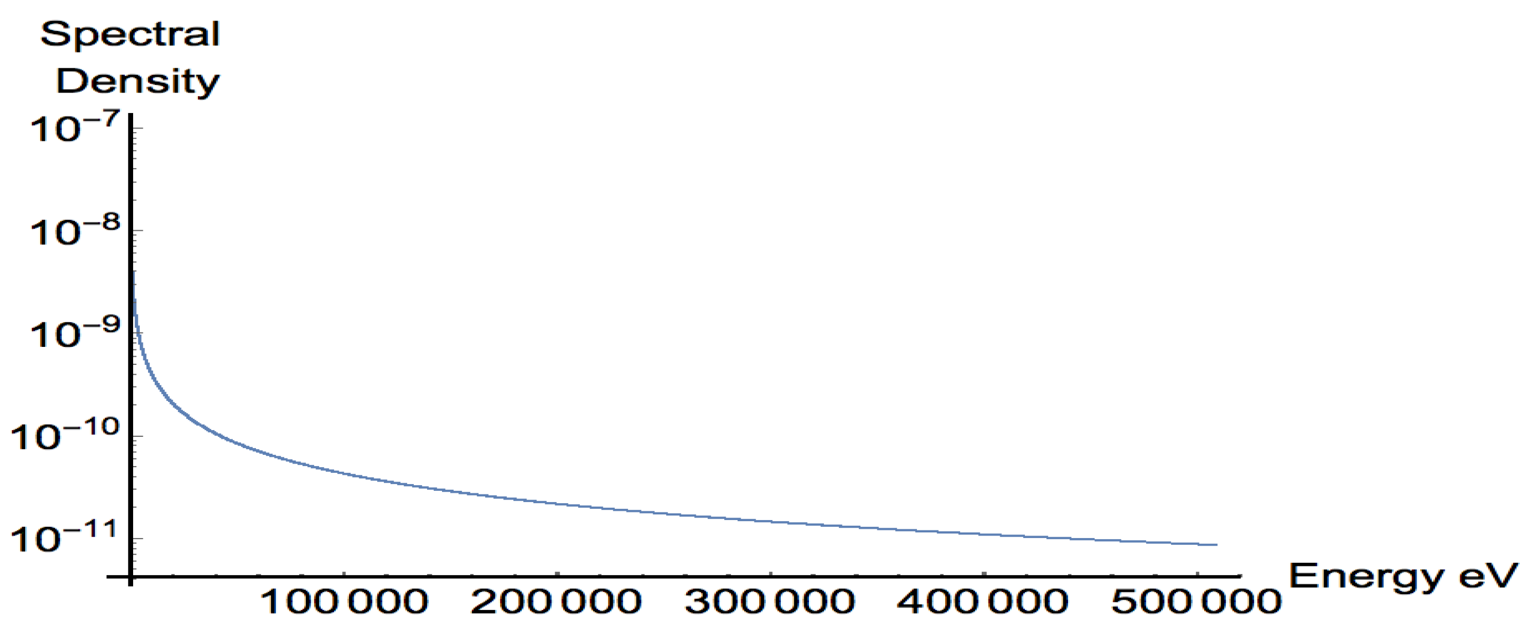
Figure 1 shows a logarithmic plot (ordinate is a log, abscissa is linear) of the spectral density $\frac{d\mathsf{\Delta }{E}_1}{dE}$ of the ground state Lamb shift with $Z=1$ over the entire range of energy E computed from Equation (29) using Mathematica. The spectral density is largest at the lowest energies, and decreases monotonically by about 4 orders of magnitude as the energy increases to 511 keV. The ground state shift is the integral of the spectral density from energy 0 to 511 keV.

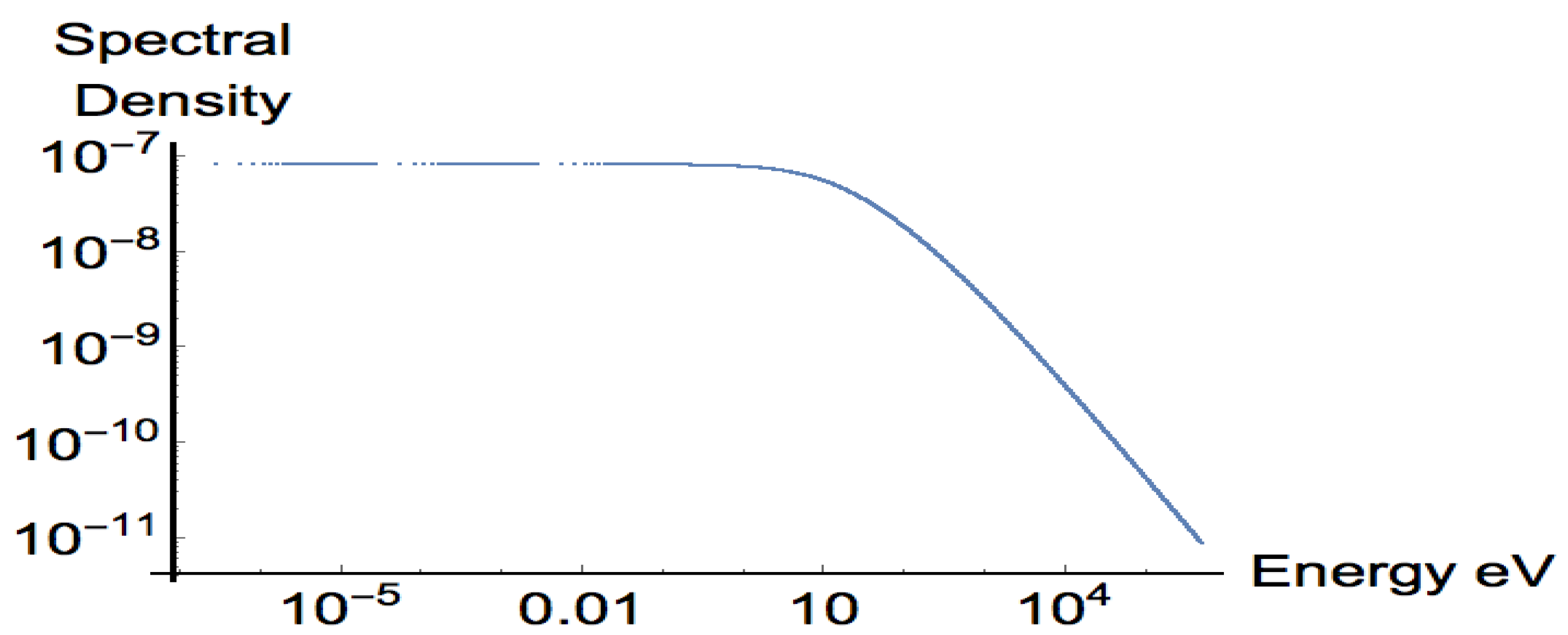
Figure 2 is a log-log plot of the same information. The use of the log-log plot expands the energy range for each decade, revealing that for energy above about 1000 eV the slope is approximately −1, indicating that the spectral density is nearly proportional to $1/E$. For energy below about 10 eV, the spectral density in Figure 2 is almost flat, corresponding to a linear decrease with E, with a maximum at the lowest energy computed, as shown in Figure 3. Figure 2 shows that there are essentially two different behaviors of the spectral density, one for values of the energy E of the vacuum field that are less than 10 eV, which is less than $E_m-E_n$, the energy difference for all bound state transitions, and another region where E is much larger than the bound state energies, and the spectral density goes as $1/E$. The origin of this behavior is clear mathematically from the factor $B=1/(E_m-E_n+E)$. In the expression for the spectral shift (6) for $E<E_m-E_n$, $B\propto 1-E/(E_m-E_n)$ and for $E>E_m-E_n$, $B\propto 1/E$.

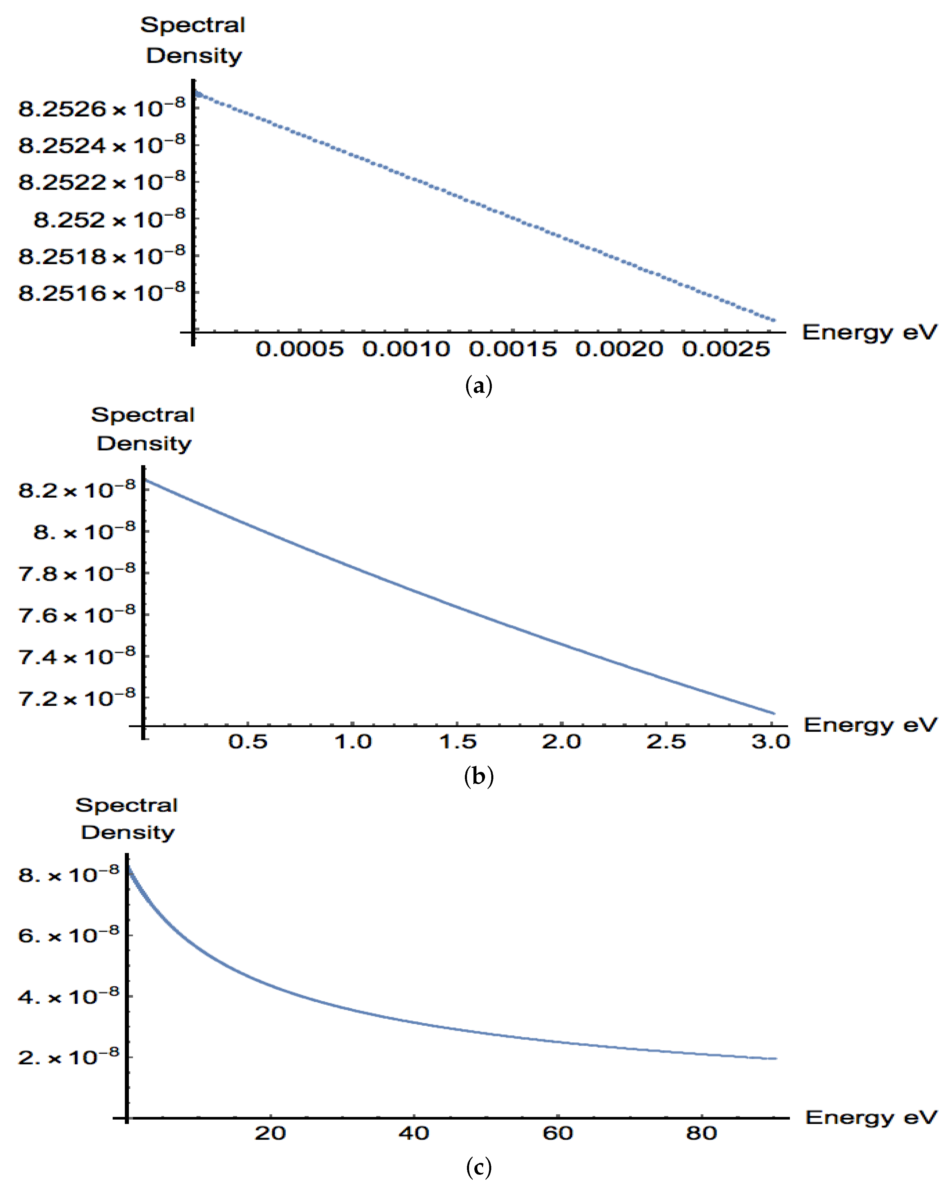
Figure 3 shows linear plots of the spectral density of the shift for the ground state computed from Equation (29) for several lower energy regions. Figure 3a shows a linear increase in the spectral density as the energy decreases over the small energy interval plotted. Figure 3b show a linear increase of about 15% as the energy decreases from 3 eV to 0 eV. Figure 3c shows that the spectral density increases by a factor of about 4 as the energy decreases from 100 eV to 0 eV. In the low-frequency limit, the spectral density increases linearly to a constant value as the energy is reduced.

From explicit evaluations, Section 4 shows that for shifts in S states with principal quantum number n, the asymptotic spectral density for large E is proportional to $\alpha {\left(Z\alpha \right)}^4(1/n^3)/E$, and Section 5 shows that as the energy E goes to zero, the spectral density increases linearly, reaching a maximum value that is proportional to $\alpha {\left(Z\alpha \right)}^2(1/n^2)$. An approximate fit to the ground state data in Figure 1 is

$$\frac{d\mathsf{\Delta }{E}_1^{\mathrm{fit}}}{dE}=D\frac{(1+e^{-HE})}{(E+C)},$$

(30)

where $D=4.4008\times {10}^{-6}$, $H=0.08445/$ eV, $C=106.79$ eV. The fit is quite good at the asymptotes and within 10% over the entire energy range.

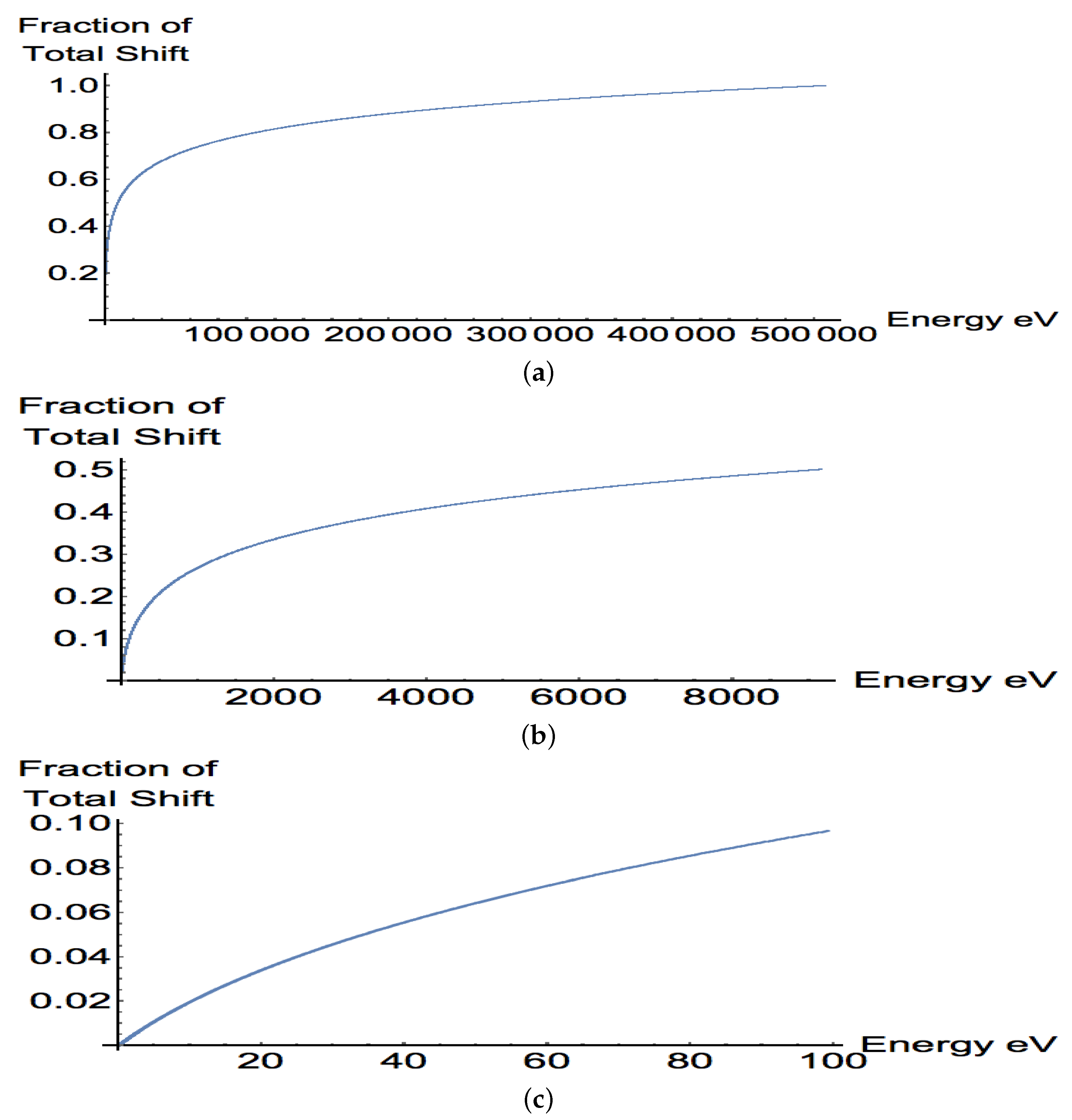
The spectral density shown in Figure 1 or Figure 2 can be used to determine the contribution to the total ground state shift from different energy regions. Integrating the spectral density from 0 eV to energy E gives the value of the partial shift ${\mathsf{\Delta }}_1\left(E\right)$ that these energies (0 eV to E eV) contribute to the total shift $\mathsf{\Delta }{E}_1$ for the ground state. In Figure 4, ${\mathsf{\Delta }}_1\left(E\right)/\mathsf{\Delta }{E}_1$, which is the fraction of the total shift $\mathsf{\Delta }{E}_1$ due to the contributions from energies below E, is plotted as a function of E. Figure 4a shows that almost 80% of the shift comes from energies below about 100,000 eV. Figure 4b shows that about half the total shift is from energies below 9050 eV. Figure 4c shows that energies below 100 eV contribute about 10% of the total shift. Energies below 13.6 eV contribute about 2.5% while energies below 1 eV contribute about 1/4% of the total. As Figure 4c shows, the fraction of the total shift increases linearly for $E<10$ eV, corresponding to the nearly horizontal portion of the shift density for $E<10$ eV, as shown in Figure 2. The contribution to the total 1S shift for the visible spectral interval 400–700 nm (1.770 eV to 3.10 eV) is about $1.00342\times {10}^{-7}$ eV or about 3/10 % of the total shift.

The relative contribution to the total shift per eV is much greater for lower energies. For example, half the 1S shift corresponds to energies 0 to 9000 eV, but only about 0.2% corresponds to 500,000 to 509,000 eV. The largest contribution to the shift per eV is at the lowest energies, which have the steepest slope of the spectral density curve in Figure 1, about 1000 times greater than the slope for the largest values of the energy. However, the total range for the large energies, from 9050 to 510,000 eV is so large that the absolute contribution to the total shift for large energies is significant.

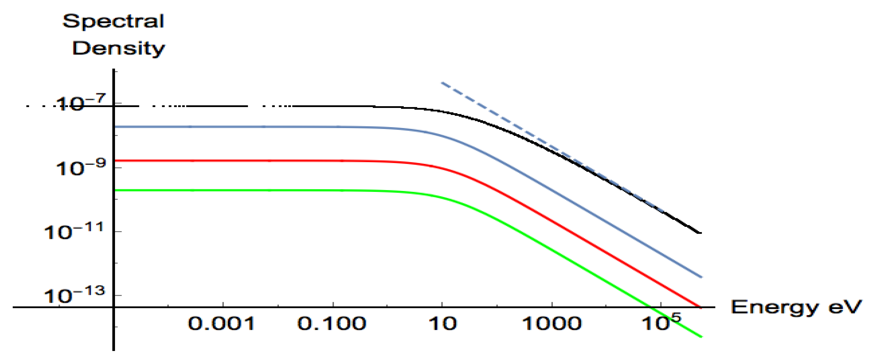
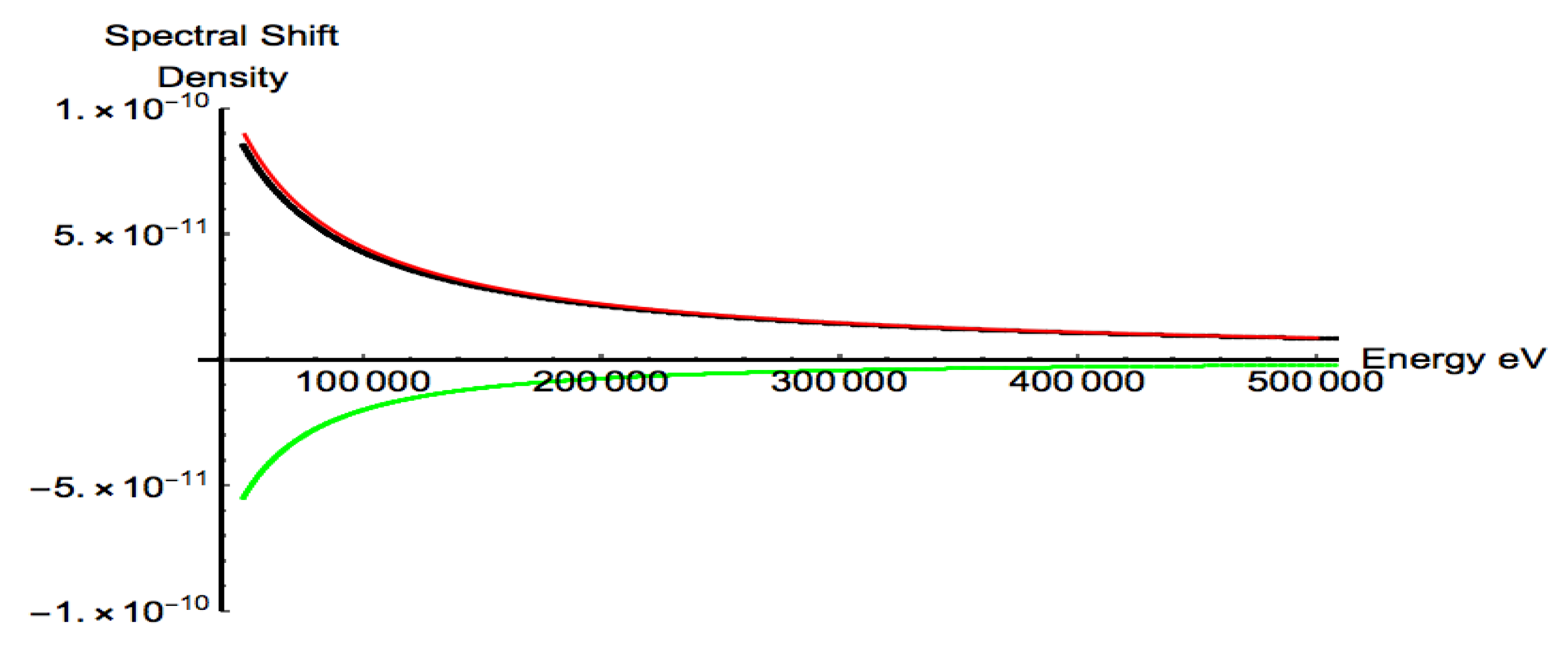
For the ground state, Figure 5 shows how the dominant terms for different m in the Bethe sum over states in Equation (6) contribute to the full spectral density obtained from group theory Equation (29). Each such term in the Bethe sum could be interpreted as corresponding to the shift resulting from virtual transitions from state n to state m occurring due to the vacuum field. Each term shown has a behavior similar to that of the full spectral density, but the magnitudes decrease as the transition probabilities decrease.

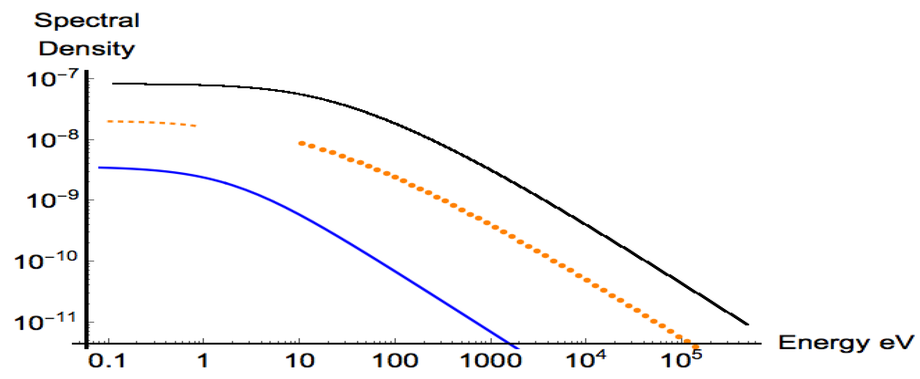
Figure 6 shows the spectral densities for 1S (black) and 2S (orange) shifts. The shapes are similar but the spectral density for the 1S shift is about eight times as large at high frequencies and about four times as large at low frequencies, factors that are derived explicitly in Section 4 and Section 5 by considering the asymptotic forms of the spectra density for S states with different principal quantum numbers. Both S states have a $1/E$ high-frequency behavior. The s-integration in the group theoretical calculation for the 2S state diverges for energies below 10.2 eV due to a non-relativistic approximation, but the spectral density of the shift can be obtained from a low-energy approximation (48) to the group theory result, which is derived in Section 5.

The spectral density $d\mathsf{\Delta }{E}_n/dE$ for a state n can be defined in a convenient form suggested by Equation (29),

$$\frac{d\mathsf{\Delta }{E}_n}{dE}=\frac{4{\alpha }^3}{3\pi }{\int }_0^{\infty }ds{W}_n(s,{\varphi }_n),{\varphi }_n=ln\left[1+\frac{E}{|E_n|}\right],$$

(31)

where the energy for state n is $E_n=-m{c}^2{\left(Z\alpha \right)}^2/2n^2$. The group theoretical results give a spectral density for the 2S–2P Lamb shift [27]:

$$W_{2S-2P}(s,{\varphi }_2)=\frac{4e^{(2s{e}^{-{\varphi }_2}+{\varphi }_2)}{sinh}^3\left({\varphi }_2\right){\csc \mathrm{h}}^2\left(\frac{s}{2}\right)}{{\left[cosh\left({\varphi }_2\right)+coth\left(\frac{s}{2}\right)\right]}^5},$$

(32)

and for the 2P shift [27]:

$$W_{2P}(s,{\varphi }_2)=-\frac{e^{(2s{e}^{-{\varphi }_2}+{\varphi }_2)}sinh\left({\varphi }_2\right){\csc \mathrm{h}}^4\left(\frac{s}{2}\right)[cosh\left({\varphi }_2\right)sinh\left(s\right)+cosh\left(s\right)-3]}{2{\left[cosh\left({\varphi }_2\right)+coth\left(\frac{s}{2}\right)\right]}^5}.$$

(33)

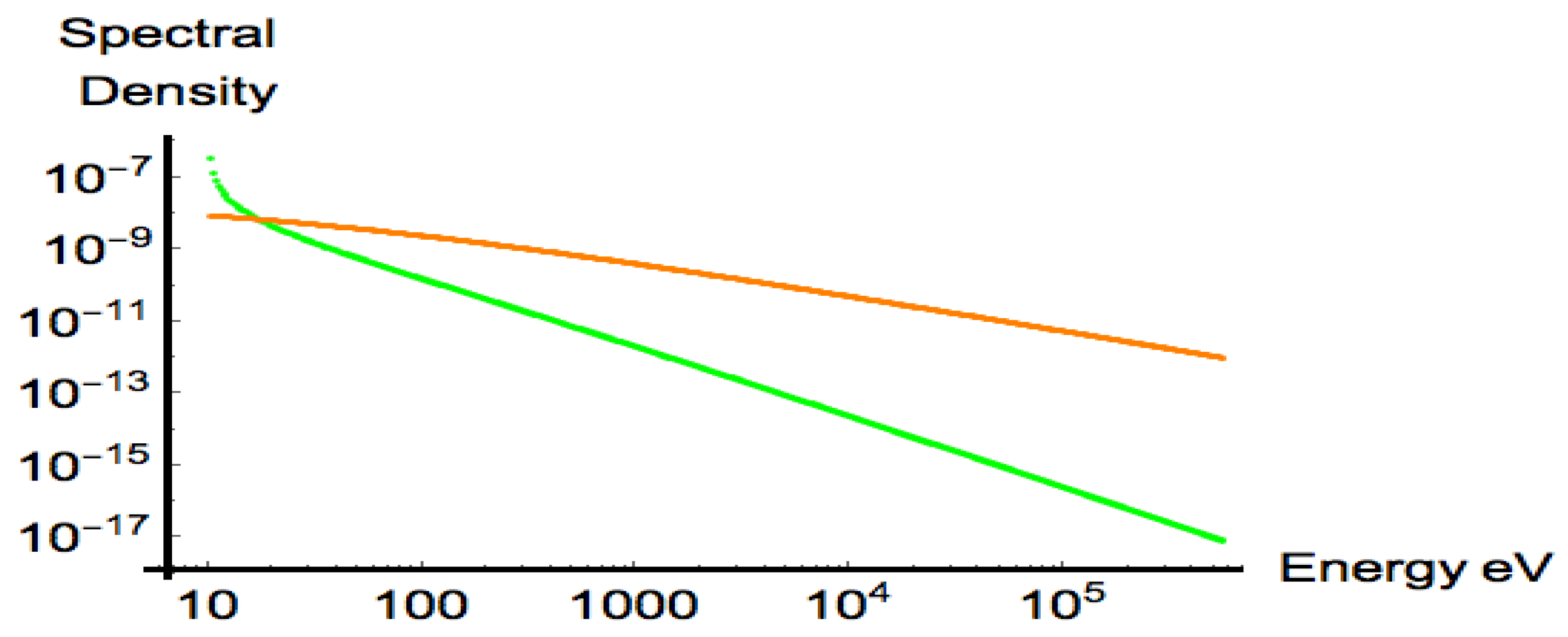
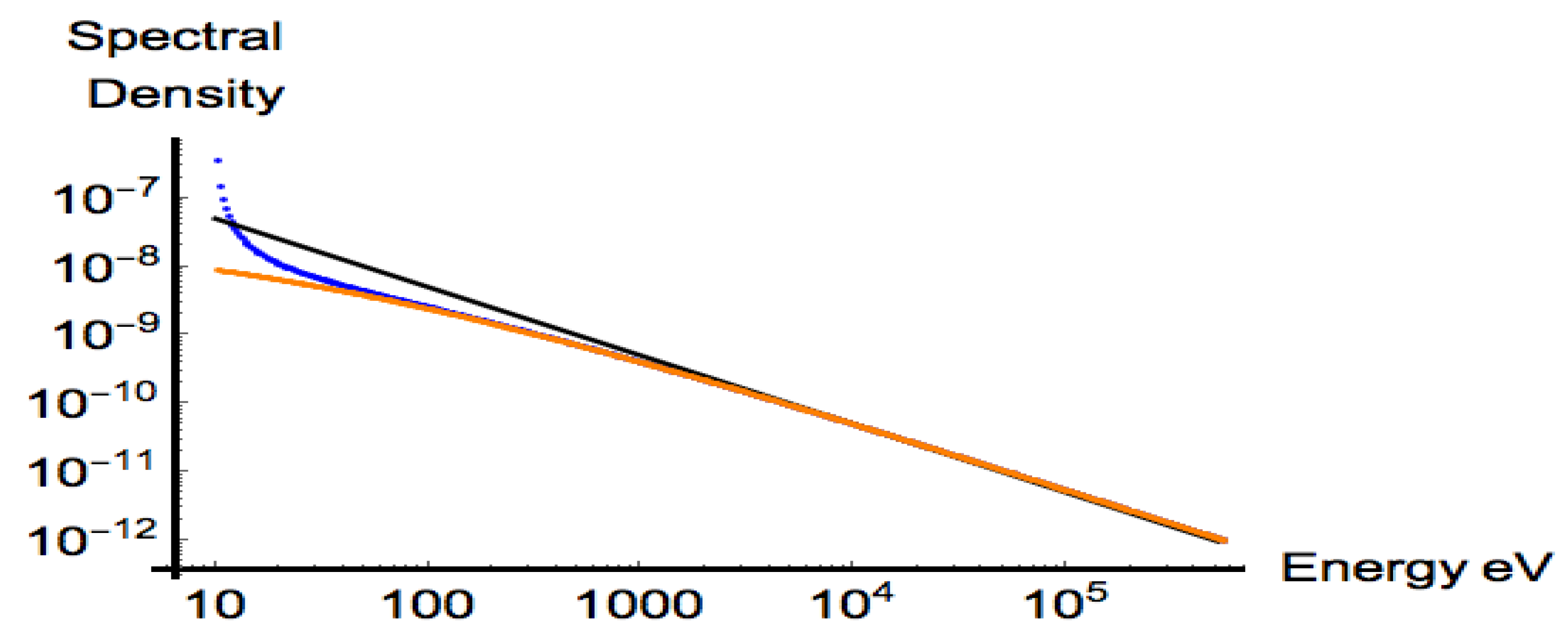
The spectral density of the 2P shift has a very different behavior from the spectral density of the 2S shift (Figure 7). It is negative and and it falls off as $1/E^2$. The shift is negative because the dominate contribution to the shift is from virtual transitions from the 2P state to the lower 1S state, with an energy difference of about 10.2 eV. For energies below about 20 eV, the absolute value of the spectral density of the 2P shift increases rapidly in magnitude as the energy is reduced and is much bigger than the spectral density for the 2S shift. The 2S shift cannot have a negative contribution from the lower 1S state since the transition 2S→1S is forbidden by the conservation of angular momentum. The classic Lamb shift arises from the difference between the two spectral densities, so the negative 2P spectral density actually increases the 2S–2P Lamb shift as the energy decreases (Figure 8). In effect, the 2S–2P shift is dominated by vacuum energies below about 100 eV. The total 2P shift is about 0.3% percent of the 2S shift. Bethe also computed a negative contribution for the shift from the 2P state [30].

Comparing the Ground State Group Theoretical Lamb Shift Calculations to Those of Bethe, Welton, and Feynman

Integrating the group theoretical spectral density Equation(29) from near zero energy $(5.4\times {10}^{-7}$ eV) to 511 keV, about the rest mass energy of the electron, gives the 1S shift of $3.4027\times {10}^{-}5$ eV, in agreement with the numerical result of Bethe and Salpeter summing over states and using the Bethe log approximation, $3.392\times {10}^{-}5$ eV, to about $0.3\%$ [8].

Bethe and Salpeter [30] reported that the ground state Bethe log, as defined in Equation 13, which is a logarithmically weighted average value of the excitation of the energy levels contributing to the radiative 1S shift, was equivalent to $|E_m-E_n{|}_{ave}$ of 19.77 Ry or 269 eV [30]. Because of the weighting, it is not clear how to interpret this value, other than it indicates that high-energy photons and scattering states contribute significantly to the shift. The group theoretical method does not provide an equivalent weighted average value for direct comparison.

Although the methods of Bethe, Welton, and Power as defined all give approximately the same value for the 1S shift, which equals the integral of the spectral density, they differ significantly in their frequency dependence, which is examined in Section 4.

4. The Spectral Density of The Lamb Shift at High Frequency

The form for $d\mathsf{\Delta }{E}_n/dE$, which is the Lamb shift spectral density for level n, can be obtained at high energies from (i) the classic calculation by Bethe using second-order perturbation theory; (ii) the calculation by Welton of the Lamb shift; (iii) the calculation by Power of the Lamb shift based on Feynman’s approach; and (iv) the group theoretical calculation.

The spectral density for level n can be written from Bethe’s expression (6):

$$\frac{\mathsf{\Delta }{E}_n^{\mathrm{Bethe}}}{\mathsf{\Delta }E}=\frac{2\alpha }{3\pi }{\left(\frac{1}{mc}\right)}^2\sum _m{\left|{\mathbf{p}}_{mn}\right|}^2(E_n-E_m)\frac{1}{E_n-E_m-E}.$$

(34)

For the ground state spectral density $n=1$, $Z=1$, $E_1=-13.613$ eV, and for the bound states with principal quantum number m, $E_m=-13.613$ eV/m². For scattering states, $E_m$ is positive. Hence the denominator is negative for all terms in the sum over m and never vanishes, and the spectral density is positive so the ground state shift is positive as it must be. For large values of E, we can make the approximation,

$$\frac{\mathsf{\Delta }{E}_n^{\mathrm{Bethe}}}{\mathsf{\Delta }E}{|}_{E\to \infty }=\frac{2\alpha }{3\pi }{\left(\frac{1}{mc}\right)}^2\sum _m{\left|{\mathbf{p}}_{mn}\right|}^2(E_m-E_n)\frac{1}{E}.$$

(35)

The summation can be evaluated using the dipole sum rule (9)–(11) for the Coulomb S state wavefunction, obtaining the final result for the high-frequency spectral density for S states with the principal quantum number, n:

$$\frac{d\mathsf{\Delta }{E}_n^{\mathrm{Bethe}}}{dE}{|}_{E\to \infty }=\frac{4m{c}^2}{3\pi }\alpha {\left(Z\alpha \right)}^4\frac{1}{n^3}\frac{1}{E}.$$

(36)

The result highlights the $1/E$ divergence at high frequencies and shows the presence of a coefficient proportional to $1/n{}^3$. To put a scale on the coefficient, the high-frequency spectral density can be written as $(8/3\pi )(\alpha {\left(Z\alpha \right)}^2/n)(E_n/E)$.

The spectral density for all frequencies from Welton’s qualitative model, Equation (17), is identical to this high-frequency limit of Bethe’s calculation. Thus, at low frequencies, the spectral density for Welton’s semi-quantitative calculation diverges as $1/E.$ Because of the expectation value of the Laplacian, Welton’s approach predicts a shift only for S states. Its appeal is that it gives a physical picture of the primary role of vacuum fluctuations in the Lamb shift and shows the presence of the $1/E$ characteristic behavior. Its treatment of bound states at low energies is incomplete and inaccurate. To obtain a level shift, it requires providing a low-energy limit for the integration. As noted previously, if the lower limit is Bethe’s log average excitation energy, 269 eV for n = 1, and the upper limit $m{c}^2$ then Welton’s total 1S shift agrees with Bethe’s. A choice of this type works since: (i) it does not include any contributions from energies below 269 eV and (ii) it gives a compensating contribution for energies from 269 eV to about 1000 eV that is larger than the actual spectral density, as shown in Figure 4 and (iii) above about 1000 eV, Welton’s model gives the same $1/E$ spectral density as Bethe.

The spectral density for Power’s model can be obtained from Equation (24):

$$\frac{\mathsf{\Delta }{E}_n^{\mathrm{Power}}}{dE}=-\frac{2\alpha }{3\pi }\frac{1}{{\left(mc\right)}^2}\sum _m{\left|{\mathbf{p}}_{mn}\right|}^2(E_m-E_n)\frac{E}{{(E_m-E_n)}^2-E^2}.$$

(37)

Letting E become large gives a result identical to the high-frequency limit (35) for the Bethe formalism and the Welton model, namely

$$\frac{\mathsf{\Delta }{E}_n^{\mathrm{Power}}}{dE}{|}_{E\to \infty }=\frac{4m{c}^2}{3\pi }\frac{\alpha {\left(Z\alpha \right)}^4}{n^3}\frac{1}{E}.$$

(38)

Thus, the models of Bethe, Welton, and Power predict S states with the same $1/E$ dependence of the high-frequency spectral density, corresponding to the logarithmic divergence at high-frequency. The asymptotic theoretical result can be written in a form allowing convenient comparison to the calculated group theoretical spectral density

$$\frac{d\mathsf{\Delta }{E}_n^{\mathrm{Bethe}}}{dE}{|}_{E\to \infty }=\frac{4m{c}^2}{3\pi }\frac{\alpha {\left(Z\alpha \right)}^4}{n^3}\frac{1}{E}.$$

(39)

The spectral density goes as $1/n^3$ for S states. For the ground state $n=1,Z=1$, this gives:

$$\frac{d\mathsf{\Delta }{E}_1^{\mathrm{Bethe}}}{dE}{|}_{E\to \infty }=4.488\times {10}^{-6}\frac{1}{E}.$$

(40)

A fit to the last two data points near 510 keV in the group theoretical calculations (GTcalc) gives:

$$\frac{d\mathsf{\Delta }{E}_1^{\mathrm{GTcalc}}}{dE}{|}_{E\to \infty }=4.4008\times {10}^{-6}\frac{1}{E}.$$

(41)

The coefficients differ by about $2\%$. Figure 9 is a plot of the ground state group theoretical calculated spectral density (red) from Equation (29) and the theoretical asymptotic behavior from Bethe, Power and Welton, Equation (40) (black), and the difference times of a factor of 10. The asymptotic theoretical result agrees with the full group theoretical calculation from Equation (29) to within about $2\%$ at 511 keV, and to about $6\%$ at 50 KeV. It is notable that the high-frequency form is a reasonable approximation down to 50 keV. Indeed, the Welton qualitative approach is based on this observation; it has the same $1/E$ energy dependence at all energies.

5. Spectral Density of the Lamb Shift at Low Frequency

To obtain a low-frequency limit of the spectral density of the Lamb shift from the Bethe spectral density (34), expand the spectral density to first-order in E, giving

$$\frac{\mathsf{\Delta }{E}_n^{\mathrm{Bethe}}}{dE}{|}_{E\to 0}=\frac{2\alpha }{3\pi }{\left(\frac{1}{mc}\right)}^2\sum _m{\left|{\mathbf{p}}_{mn}\right|}^2\left(1-\frac{E}{E_m-E_n}\right).$$

(42)

Since the sum is over a complete set of states m, including scattering states, the first term in parenthesis can be evaluated using the sum rule,

$$\sum _m{\left|{\mathbf{p}}_{mn}\right|}^2=-2m{E}_n={\left(mc\right)}^2\frac{{\left(Z\alpha \right)}^2}{n^2}.$$

(43)

To evaluate the second term, Equation (22) and the Thomas–Reiche–Kuhn sum rule [31] can be used, giving

$$\sum _m{\omega }_{mn}{\left|{\mathbf{d}}_{mn}\right|}^2=\frac{3e^2\hslash }{2m}.$$

(44)

The final result for $E\to 0$ is

$$\frac{\mathsf{\Delta }{E}_n^{\mathrm{Bethe}}}{dE}{|}_{E\to 0}=\frac{2\alpha }{3\pi }\frac{{\left(Z\alpha \right)}^2}{n^2}-\frac{\alpha }{\pi m{c}^2}E.$$

(45)

The corresponding spectral density for $n=1,Z=1$, is

$$\frac{d\mathsf{\Delta }{E}_1^{\mathrm{Bethe}}}{dE}{|}_{E\to 0}=\frac{4\alpha \times 13.6}{3\pi m{c}^2}\left(1-\frac{3E}{4\times 13.6}\right)=8.253\times {10}^{-8}(1-0.0551E).$$

(46)

As E decreases to zero, the spectral density increases linearly to a constant value,

$$4\alpha |E_n|/3\pi m{c}^2=2{\alpha }^3{Z}^2/3\pi n^2=8.253\times {10}^{-8}/n^2.$$

The intercept goes as $1/n^2$, but the slope is $\alpha /\pi m{c}^2$, which has a remarkably simple form and is independent of n.

Taking the low-frequency limit of the group theoretical result analytically gives exactly the same result as Equation (45) from the Bethe formulation:

$$\frac{d\mathsf{\Delta }{E}_1^{\mathrm{GTcalc}}}{dE}{{|}_{E\to 0}=\frac{d\mathsf{\Delta }{E}_1^{\mathrm{Bethe}}}{dE}|}_{E\to 0}=\frac{2\alpha }{3\pi }\frac{{\left(Z\alpha \right)}^2}{n^2}-\frac{\alpha }{\pi m{c}^2}E.$$

(47)

Figure 3 shows the results of group theoretical calculations of the spectral density of the ground state Lamb shift for different energy regions, showing the near linear increase in the spectral density as the frequency decreases from 80 eV to ${10}^{-5}$ eV. For low values of E, the slopes and intercept agree with Equation (47) within about two tenths of a percent.

To explore Power’s approach at low frequencies, let E become small in the spectral density Equation (37), giving

$$\frac{\mathsf{\Delta }{E}_n^{\mathrm{Power}}}{dE}{|}_{E\to 0}=-\frac{2NV}{3\pi c^3}\sum _m{\left|{\mathbf{p}}_{mn}\right|}^2\frac{E}{E_m-E_n},$$

(48)

which is identical to the second term in the low E approximation to the Bethe result (45) so

$$\frac{\mathsf{\Delta }{E}_n^{\mathrm{Power}}}{dE}{|}_{E\to 0}=-\frac{1}{\pi }\frac{\alpha }{m{c}^2}E.$$

(49)

The result Equation (49) is identical to the frequency-dependent term in Equation (47) which is the low-frequency spectral density from the Bethe approach and from the group theoretical expression. However, in the low-frequency limit based on Power’s expression for the spectral density, the constant term that is present in the other approaches does not appear. This is a consequence of the form used for the index of refraction, which assumes that real photons are present that can excite the atom with resonant transitions. More sophisticated implementations of Feynman’s proposal may avoid this issue.

6. Comparison of the Spectral Energy Density of the Vacuum Field and the Spectral Density of the Radiative Shift

The theory of Feynman proposes that the vacuum energy density in a large box containing H atoms, which are assumed to be in the 1S ground state, increases uniformly with the addition of the atoms. Feynman maintains that the total vacuum energy in the box increases by the Lamb shift times the number of atoms present [6,10]. If there were only one atom in a very large box, one would not expect the change in energy density to be spatially uniform but more concentrated near the atom. To develop a model of the spatial dependence of the change in energy density for one atom, the close relationship between the vacuum field and the radiative shift can be used. The spectral densities of the ground state shift and of the quantum vacuum with no H atoms present are both known. In the box, the vacuum field density must increase so that the integral gives the 1S Lamb shift. The spectral energy density of the vacuum field with no H atom present is equal to [6]

$${\rho }_0\left(\omega \right)=\frac{\hslash {\omega }^3}{2{\pi }^2{c}^3},$$

(50)

where c is in cm/sec and $\omega$ is in sec⁻¹. If frequency is measured in eV, so $\hslash \omega =E$, then the vacuum spectral energy density in 1/$cc$ is

$${\rho }_0\left(E\right)=\frac{E^3}{2{\pi }^2{\hslash }^3{c}^3},$$

(51)

and ${\int }_{E_1}^{E_2}{\rho }_0\left(E\right)dE$ would be the energy density eV/$cc$ in the energy interval $E_1$ to $E_2$. The question being addressed is: what volume of vacuum energy of density ${\rho }_0\left(E\right)$ is required to supply the amount of energy needed for the radiative shift? The total radiative shift $\mathsf{\Delta }{E}_1$ be expressed as the integral of the vacuum energy density ${\rho }_0\left(E\right)$ over an effective volume $V_1\left(E\right)$,

$$\mathsf{\Delta }{E}_1={\int }_0^{m{c}^2}dE{\rho }_0\left(E\right)V_1\left(E\right),$$

(52)

where the same upper limit for E is used as in previous calculations. Recall the definition (28) of the spectral shift:

$$\mathsf{\Delta }{E}_1={\int }_0^{m{c}^2}dE\frac{\mathsf{\Delta }{E}_1}{dE}.$$

(53)

Comparing Equations (52) and (53) and insuring the energy balance at each energy E, gives the effective spectral volume $V_1\left(E\right)$

$$V_1\left(E\right)=\frac{d\mathsf{\Delta }{E}_1}{dE}\frac{1}{{\rho }_0\left(E\right)}.$$

(54)

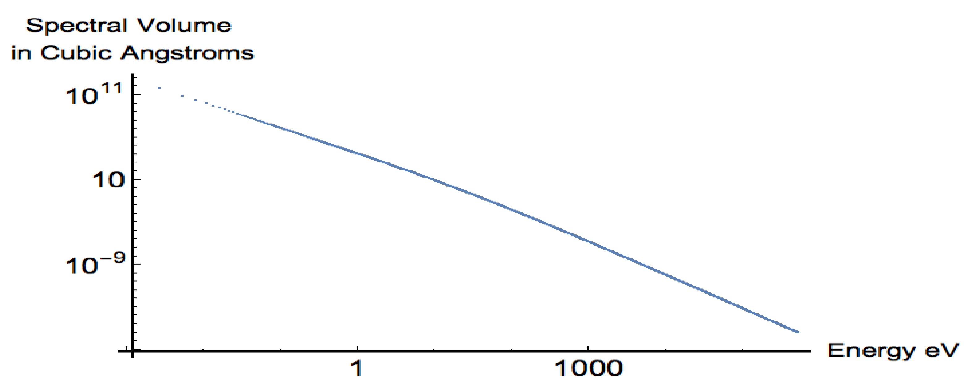
The spectral volume $V_1\left(E\right)$ has the dimensions of $cc$ and contains the amount of vacuum energy at energy value E that corresponds to the ground state spectral density at the same energy E. In Figure 10, for the 1S ground state radiative shift, the log of the spectral volume $V_1\left(E\right)$, in cubic Angstroms (Å${}^3$), is plotted versus the log of the energy, E.

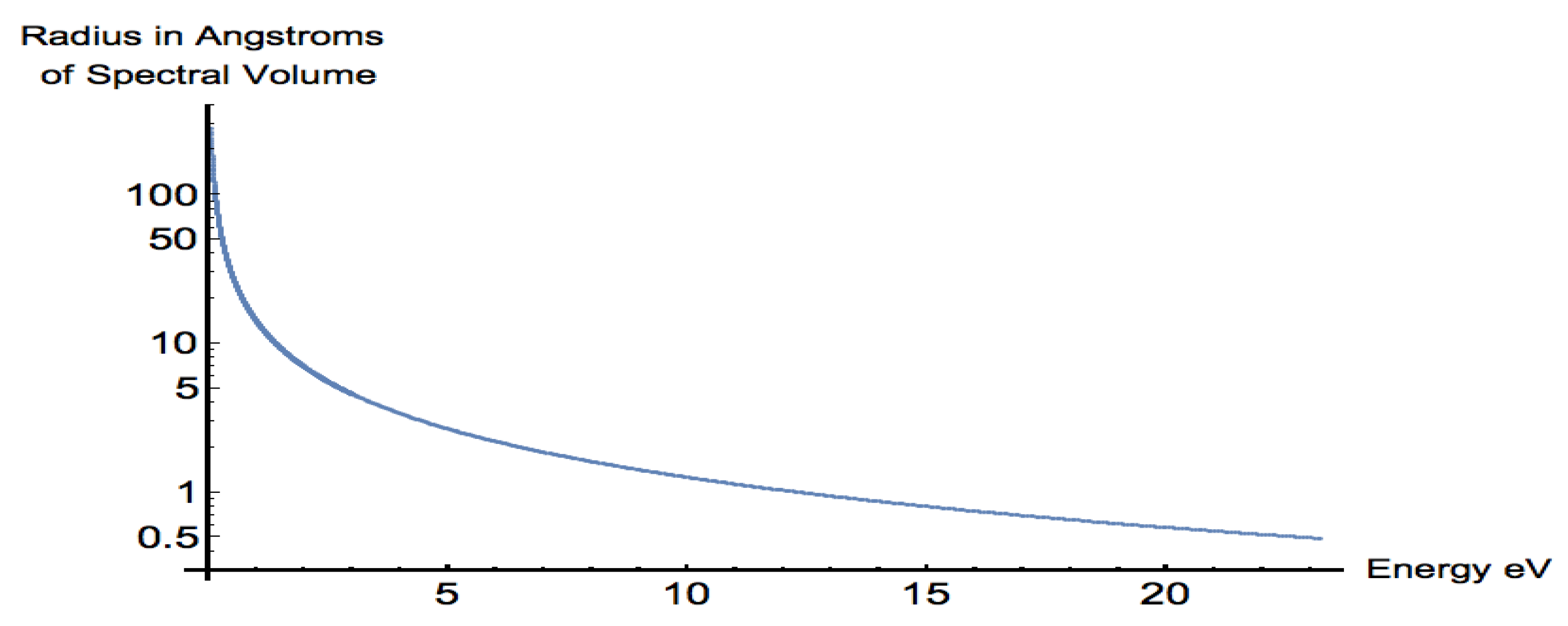
For energies above about 100 eV, the spectral volume is less than 1 Å${}^3$, approximately the volume of the ground state wavefunction. For an energy of 1 eV, the spectral volume is 11850 Å${}^3$, corresponding to a sphere of radius about 14 Å. This calculation predicts that there is a sphere of positive vacuum energy of radius 14 Åaround the atom corresponding to the 1 eV shift spectral density. Figure 11 shows the radius of the spherical spectral volume $V_1\left(E\right)$ for energies from 0.05 eV, with spectral radius of 278 Å, to 23 eV, with radius 0.49 Å.

7. Conclusions

The non-relativistic Lamb shift can be interpreted as due to the interaction of an atom with the fluctuating electromagnetic field of the quantum vacuum. We introduce the concept of a spectral shift density which is a function of frequency $\omega$ or energy $E=\hslash \omega$ of the vacuum field. The integral of the spectral density from $E=0$ to the rest mass energy of an electron, 511 keV, gives the radiative shift. We report on calculations of the spectral density of the level shifts for 1S, 2S and 2P states based on a group theoretical analysis and compare the results to the spectral densities implicit in previous non-relativistic calculations of the Lamb shift by Bethe, Welton, and Power. The group theoretical calculation provides an explicit form for the spectral density over the entire spectral range with no summation over intermediate states. Bethe’s approach requires a summation over an infinite number of states, including all bound and all scattering states, to obtain a comparable spectral density. The different approaches for asymptotic cases, for very large and very small energies E, are compared.

The calculations of the shift spectral density provide a new perspective on radiative shifts. The group theory approach as well as the approaches of Bethe, Power, and Welton all show the same $1/E$ high-frequency behavior for S states above about $E=\hslash \omega$ = 1000 eV to 511 keV, namely an asymptotic spectral density for S states equal to $(4/3\pi )(\alpha {\left(Z\alpha \right)}^{4}m{c}^2/n^3)(1/E)$ for principal quantum number n. The group theory calculation shows that about 76% of the ground state 1S shift is contributed by E above 1000 eV, which is essentially why all the approaches give approximately the same result for the 1S Lamb shift.

Only the Bethe and group theory calculations have the correct low-frequency behavior. For S states the spectral density increases linearly as E decreases to zero. Its maximum value is at $E=0$ and for S states equals $(2\alpha /3\pi ){\left(Z\alpha \right)}^2/\left(n^2\right)$. This maximum value is about $1/{\left(Z\alpha \right)}^2$ or about $2\times {10}^4$ larger than the high-frequency spectral density at $E=511$ keV. Thus, low energies contribute much more to the shift for a given spectral interval than high energies. Energies below 13.6 eV contribute about 2.5 %. Because of the huge spectral range contributing to the shift, contributions to the shift from high energies are very important. Half the contribution to the 1S shift is from energies above 9050 eV.

The 2P shift has a very different spectral density from an S state: it is negative and has an asymptotic behavior that goes as $1/E^2$ rather than as $1/E$. Below about 20 eV, the absolute value of the 2P spectral density is much larger than the 2S spectral density and it dominates the 2S–2P shift spectral density, yet the total 2P shift is only about 0.3% of the total 2S shift.

References

- Choudhuri, A.R. Astrophysics for Physicists; Cambridge University Press: Cambridge, UK, 2010. [Google Scholar]
- Carroll, S.M. Addressing the quantum measurement problem. Phys. Today 2022, 75, 62–64. [Google Scholar] [CrossRef]
- D’Espagnat, B. Veiled Reality: An Analysis of Present-Day Quantum Mechanical Concepts; CRC Press/Taylor & Francis Group: Boca Raton, FL, USA, 2013. [Google Scholar] [CrossRef]
- Beyer, A.; Maisenbacher, L.; Matveev, A.; Pohl, R.; Khabarova, K.; Grinin, A.; Lamour, T.; Yost, D.C.; Hänsch, T.W.; Kolachevsky, N.; et al. The Rydberg constant and proton size from atomic hydrogen. Science 2017, 358, 79–85. [Google Scholar] [CrossRef] [PubMed] [Green Version]
- Berestetskii, V.B.; Lifshitz, E.M.; Pitaevskii, L.P. Quantum Electrodynamics. Course of Theoretical Physics: Volume 4, Second Edition; Pergamon Press: Oxford, UK, 1982. [Google Scholar] [CrossRef] [Green Version]
- Milonni, P.W. The Quantum Vacuum. An Introduction to Quantum Electrodynamics; Academic Press, Inc.: San Diego, CA, USA, 1994. [Google Scholar] [CrossRef]
- Lamb, W.E.; Retherford, R.C. Fine tructure of the hydrogen atom by a microwave method. Phys. Rev. 1947, 72, 241–243. [Google Scholar] [CrossRef]
- Bethe, H.A. The electromagnetic shift of energy levels. Phys. Rev. 1947, 72, 339–341. [Google Scholar] [CrossRef]
- Welton, T.A. Some observable effects of the quantum-mechanical fluctuations of the electromagnetic field. Phys. Rev. 1948, 74, 1157–1168. [Google Scholar] [CrossRef]
- Power, E.A. Zero-point energy and the Lamb shift. Am. J. Phys. 1966, 34, 516–518. [Google Scholar] [CrossRef]
- Compagno, G.; Passante, R.; Persico, F. Atom-Field Interactions and Dressed Atoms; Cambridge University Press: Cambridge, UK, 1995. [Google Scholar] [CrossRef]
- Maclay, G.J. History and some aspects of the Lamb shift. Physics 2020, 2, 105–149. [Google Scholar] [CrossRef] [Green Version]
- Dyson, F.J. The electromagnetic shift of energy levels. Phy. Rev. 1948, 73, 617–626. [Google Scholar] [CrossRef]
- French, J.B.; Weisskopf, V.F. The electromagnetic shift of energy levels. Phys. Rev. 1949, 75, 1240–1248. [Google Scholar] [CrossRef]
- Kroll, N.M.; Lamb, W.E., Jr. On the self-energy of a bound electron. Phys. Rev. 1949, 75, 388–398. [Google Scholar] [CrossRef]
- Weinberg, S. The Quantum Theory of Fields. Volume 1: Foundations; Cambridge University Press: Cambridge, UK, 1995. [Google Scholar] [CrossRef]
- Erickson, G.W.; Yennie, D.R. Radiative level shifts, I. Formulation and lowest order Lamb shift. Ann. Phys. 1965, 35, 271–313. [Google Scholar] [CrossRef]
- Schwinger, J. Quantum electrodynamics. I. A covariant formulation. Phy. Rev. 1948, 74, 1439–1461. [Google Scholar] [CrossRef]
- Feynman, R.P. The development of the space-time view of quantum electrodynamics. Phys. Today 1966, 19, 31–44. [Google Scholar] [CrossRef] [Green Version]
- Dyson, F.J. The radiation theories of Tomonaga, Schwinger, and Feynman. Phys. Rev. 1949, 75, 486–502. [Google Scholar] [CrossRef]
- Akhiezer, A.I.; Berestetskiĭ, V.B. Quantum Electrodynamics; Interscience Publishers/John Wiley and Sons, Inc.: New York, NY, USA, 1965; Available online: https://archive.org/details/akhiezer-berestetskii-quantum-electrodynamics/page/n7/mode/2up (accessed on 30 August 2022).
- Itzykson, C.; Zuber, J.-B. Quantum Field Theory; McGraw-Hill Inc.: New York, NY, USA, 1980. [Google Scholar]
- Grotch, H. Status of the theory of the Hydrogen Lamb shift. Found. Phys. 1994, 24, 249–272. [Google Scholar] [CrossRef]
- Feynman, R.P. The present status of quantum electrodynamics. In Proceedings of the 12th La Théorie Quantique des Chomps. Douziéme Conseil de Physique, Brussels, Belgium, 9–14 October 1961; Stoops, R., Ed.; Interscience Publishers/John Wiley and Sons, Inc.: New York, NY, USA, 1962; pp. 61–99. Available online: http://www.solvayinstitutes.be/html/solvayconf_physics.html (accessed on 30 August 2022).
- Lieber, M. O(4) symmetry of the hydrogen atom and the Lamb shift. Phy. Rev. 1968, 174, 2037–2054. [Google Scholar] [CrossRef]
- Huff, R.W. Simplified calculation of Lamb shift using algebraic techniques. Phys. Rev. 1969, 186, 1367–1379. [Google Scholar] [CrossRef]
- Maclay, G.J. Dynamical symmetries of the H atom, one of the most important tools of modern physics: SO(4) to SO(4,2), background, theory, and use in calculating radiative shifts. Symmetry 2020, 12, 1323. [Google Scholar] [CrossRef]
- Brown, L.S. Bounds on screening corrections in beta decay. Phys. Rev. 1964, 135, B314–B319. [Google Scholar] [CrossRef]
- Schweber, S.S. QED and the men who made it: Dyson, Feynman, Schwinger, and Tomonaga; Princeton University Press: Princeton, NJ, USA, 1994. [Google Scholar]
- Bethe, H.A.; Salpeter, E.E. The Quantum Mechanics of One- and Two-Electron Atoms; Springer-Verlag: Berlin/Heidelberg, Germany, 1957. [Google Scholar] [CrossRef]
- Sakurai, J.J. Modern Quantum Mechanics; Addison-Wesley Publishing Company, Inc.: New York, NY, USA, 1994; Available online: https://www.fisica.net/mecanica-quantica/Sakurai%20-%20Modern%20Quantum%20Mechanics.pdf (accessed on 30 August 2022).
- Morse, P.M.; Feshbach, H. Methods of Theoretical Physics; McGraw-Hill Book Company, Inc.: New York, NY, USA, 1953; Volume 2. [Google Scholar]
Figure 1.
Plot of the log of the spectral density of the ground state Lamb shift from the group theoretical expression (29) versus the energy from 0 to 510 keV.
Figure 2.
Log-log plot of the spectral density of the ground state shift from the group theoretical expression (29) versus the energy. For energies above about 1000 eV, the behavior is dominated by a 1/energy dependence. From about 10 eV to 0 eV, there is a slow linear increase in the spectral density.
Figure 3.
Linear plots of the ground state spectral density calculated from group theory as a function of energy for low and mid energies. From about 10 eV to 0 eV, the spectral density increases linearly to its maximum value. The value of the abscissa at the origin is 0 eV for all graphs. (a): Linear change in ground state spectral density at very low energies. (b): Near linear change in ground state spectral density for visible and near infra-red energies. The contribution to the total shift for energies below 3 eV is about 0.7%. (c): Ground state spectral density calculated for energies below 80 eV, which contribute about to the total shift.
Figure 4.
The ordinate is the fraction of the ground state shift due to vacuum field energies between 0 and E, plotted as a function of E. This plot is obtained by integration of the spectral density Equation (29), shown in Figure 1. The plot is linear in the ordinate and abscissa. The origin corresponds to (0,0) for all plots. (a): Fraction of the 1S shift due to energies from 0 to E for keV. (b): Fraction of the 1S shift due to energies below E, for eV. (c): Fraction of the 1S shift due to energies from 0 to E, for eV. Energies below 30 eV account for about 0.05 of the total shift. The variation is linear for eV.
Figure 5.
Log-log plot of the 1S spectral density from group theory Equation (29) in black, and the contributions to this shift in the Bethe formalism for the transition (blue), (red), (green). The dashed blue line shows the high-frequency asymptote. The black line is the complete spectral density which is the summation of the contributions from all transitions.
Figure 6.
A log-log plot of the group theoretical spectral density for the 1S (black) and 2S (orange) shifts versus energy. The dashed orange curve below 1 eV is a 2S low-energy approximation (47) from group theory or the Bethe formula. The blue is the largest single contribution in the Bethe formalism to the 2S shift for the transition .
Figure 7.
Log-log plot of the absolute value of the spectral density versus the energy for the 2S shift (orange), which goes as for large E, and for the 2P shift (green), which goes as for large E. At 511 keV, the 2P spectral density is about 5 orders of magnitude smaller than the 2S spectral density. Below 20 eV, the absolute value of the 2P spectral density is greater than the 2S spectral density. Note that the 2P spectral density is actually negative and the 2S spectral density is positive.
Figure 8.
Log-log plot of the spectral density for the 2S shift (orange) and the 2S–2P Lamb shift (blue) versus energy. The solid black line is the asymptote.
Figure 9.
Top red curve is the 1S group theoretical calculated spectral density (29), slightly lower black curve is the asymptotic model Equation (39), and the bottom green curve is the difference times 10, plotted for the interval 50–510 keV. Both axes are linear.
Figure 10.
Log-log plot of the spectral volume as a function of E. The spectral volume contains the free field vacuum energy at energy value E that corresponds to the ground state shift spectral density at the same energy E.
Figure 11.
Log of the radius of the spherical spectral volume , as a function of the vacuum field energy E, from 0.05 eV to 23 eV.
Publisher’s Note: MDPI stays neutral with regard to jurisdictional claims in published maps and institutional affiliations. |
© 2022 by the author. Licensee MDPI, Basel, Switzerland. This article is an open access article distributed under the terms and conditions of the Creative Commons Attribution (CC BY) license (https://creativecommons.org/licenses/by/4.0/).
Share and Cite
MDPI and ACS Style
Maclay, G.J. New Insights into the Lamb Shift: The Spectral Density of the Shift. Physics 2022, 4, 1253-1277. https://doi.org/10.3390/physics4040081
AMA Style
Maclay GJ. New Insights into the Lamb Shift: The Spectral Density of the Shift. Physics. 2022; 4(4):1253-1277. https://doi.org/10.3390/physics4040081
Chicago/Turabian StyleMaclay, G. Jordan. 2022. "New Insights into the Lamb Shift: The Spectral Density of the Shift" Physics 4, no. 4: 1253-1277. https://doi.org/10.3390/physics4040081