
Assessing Quantum Calculation Methods for the Account of Ligand Field in Lanthanide Compounds

1
Institute of Physical Chemistry, Splaiul Independentei 202, 060041 Bucharest, Romania
2
Department of Physics, Ovidius University of Constanta, 900527 Constanta, Romania
*
Author to whom correspondence should be addressed.
Physchem 2023, 3(2), 270-289; https://doi.org/10.3390/physchem3020019
Submission received: 5 May 2023
/
Revised: 1 June 2023
/
Accepted: 7 June 2023
/
Published: 16 June 2023
(This article belongs to the Section Theoretical and Computational Chemistry)
Abstract
:We obtained thorough insight into the capabilities of various computational methods to account for the ligand field (LF) regime in lanthanide compounds, namely, a weakly perturbed ionic body and quasidegenerate orbital multiplets. The LF version of the angular overlap model (AOM) was considered. We intentionally took very simple idealized systems, the hypothetical [TbF]2+, [TbF2]+ and [Tb(O2NO)]2+, in order to explore the details overlooked in applications on complex realistic systems. We examined the 4f and 5d orbital functions in connection to f–f and f–d transitions in the frame of the two large classes of quantum chemical methods: wave function theory (WFT) and density functional theory (DFT). WFT methods are better suited to the LF paradigm. In lanthanide compounds, DFT faces intrinsic limitations because of the frequent occurrence of quasidegenerate ground states. Such difficulties can be partly encompassed by the nonstandard control of orbital occupation schemes. Surprisingly, we found that the simplest crystal field electrostatic approximation, reconsidered with modern basis sets, works well for LF parameters in ionic lanthanide systems. We debated the largely overlooked holohedrization effect that inserts artificial inversion symmetry into standard LF Hamiltonians.
1. Introduction
In this study, we considered computational experiments in different technical settings, investigating the title problem and retaining the conceptual beacon ideas of ligand field (LF) theories. The LF represents a class of phenomenological models, proposing parameters for the split of atomic orbitals (d for transition metal compounds [1] or f-type for lanthanide ions [2]) in specific environments from molecules and crystals. Initially, in historical versions, due to Bethe and van Vleck [3,4], it was thought that perturbation can be estimated from first principles if it is considered to be mostly electrostatic. Practice, acquired mostly from the spectroscopy of transition metal ions [5], showed that the electrostatic simple hypothesis did not work well, but the LF models were fruitful after making all parameters adjustable, fitted from experimental spectra. The term ‘ligand field’ is also encountered under another name, ‘crystal field’ (CF) [2]. Here, we would like to use the term ‘CF’ for situations when the parameters are taken by electrostatic models, similar to early ideas.
Long before the computer era of molecular or solid-state electronic structure codes, the LF paradigm was the sole route to the examination of the quantum effects of d or f electrons. Currently, the LF is used as a tool for interpreting and validating the results of brute-force calculations [6,7].
The LF Hamiltonian in the Wybourne formulation [8] is as follows:
Here, Yk,q = Yk,q(θ, φ) are spherical harmonics, the explicit dependence on polar angles being dropped in the above description. The LF potential operator takes a matrix representation on the basis of the considered atomic orbitals (i.e., l = 2 for transition metals, or l = 3 for lanthanides):
Instead of complex spherical harmonics, we can work with the real angular parts of the orbitals, converting the and conjugate couples into the real sine and cosine components, and , respectively.
Designs with spherical harmonics are convenient because these Hamiltonian matrices must be integrated with atomic orbitals (AOs) that pertain to a shell with a given secondary quantum number, l. Then, the integrals from Equation (2) contain Y*l,m·Yk,q·Yl,m’ products, with the left- and right-side factors coming from AO definitions (the “bra” and “ket” functions); the middle factor comes from the Hamiltonian matrix. The use of even k indices, k = 0, 2, … 2l is determined via algebraic rules in order to have nonvanishing integrals [9]. The k = 0 component, which causes an overall shift in the diagonal of the LF Hamiltonian matrix and the resulted eigenvalues, is omitted from Equation (1), where the summation starts at k = 2. This means that the Hamiltonian representation is traceless, with the sum of diagonal elements and eigenvalues being zero, i.e., having the energy spectrum shifted in its barycenter, as a matter of convention.
The somewhat complicated expansion of Equation (1) pays tribute to the historical development of this field. Otherwise, the above formulation is quite trivial because it generally proposes just as many parameters as in a Hamiltonian matrix written for a given l shell. For instance, with f orbitals, the LF matrix has 7 × 7 dimensions and 7·8/2 = 28 general elements (i.e., taking the diagonal and half of the matrix from below or above the diagonal because the transposed elements are the complex conjugate of the selected set). Making the matrix traceless reduces the general degrees of freedom to 27, in the absence of any symmetry (C1 point group). In Equation (1), the k = 2, 4 and 6 sums comprise 2k + 1 elements, having the 5, 9, and 13 lengths, respectively, leading to a total of 27 general parameters. When the problem has symmetry, the number of effective parameters is reduced, imposing certain ratios between the values and determining the vanishing of the other ones.
We do not discuss the subtleties of Wybourne-type LF Hamiltonians here but simply state that the number of expected independent parameters is equal to the number of totally symmetric representations selected from the reduction of k = 2, … 2l spherical harmonic sets in the given point group. This is a basic requirement because a well-designed effective Hamiltonian should remain invariant to group operations. As an example, let us consider the Oh point group. Here, k = 2 (quadrupole) behaves as Eg + T2g, yielding no contribution to the LF operator because no A1 is included. k = 4 (hexadecapole) yields A1g + Eg + T1g + T2g; k = 6 (64-pole) corresponds to A1g + A2g + Eg + T1g + 2T2g. These two sets contribute equally, with an independent parameter [10]. Here, there is an established proportionality between parameters such that only can be taken as an independent term. Similarly, the k = 6 set ends with only two LF parameters for the f shell in octahedral symmetry, and . For the d shell, which is confined to the k = 4 set, there is only one LF parameter, , proportional to the well-known 10Dq gap. In the absence of symmetry, the active k-type spherical harmonic operators are trivially decomposed in (2k + 1)·A1 totally symmetric elements, making each an independent parameter.
There are several other versions of the LF beyond the above-described Wybourne parameterization, a very intuitive one being the angular overlap model (AOM) [11,12,13,14,15,16,17,18,19]. The AOM was enthusiastically embraced by chemists dealing with d-type coordination chemistry and spectroscopy given its transparency virtues. For the f electrons, it was pioneered by W. Urland [20], which remained lesser known because of the more complicated algebraic apparatus and confinement to the somewhat exotic lanthanide chemistry. The AOM does not make the Hamiltonian operator explicit, directly parameterizing the LF matrix with the help of parameters assigned to the ligand L and bonding type (λ = σ, π, …):
where the D values are functions of φL and θL polar coordinates of the coordinated ligand (in a frame centered on the metal ion), having well-defined expressions for the l-type shell to which the LF problem refers. An alternative model was advanced by Malta [21], mixing AOM-like terms assigned to chemical bonding with electrostatic terms. Recent works and reviews [22,23] have proven the current interest in AOM on lanthanide compounds in connection with modern applications of these materials in new light-emission technologies [24,25,26].
Because we revisit the LF ideas with modern tools, the following part of the Introductory is devoted to state-of-the-art computational chemistry. There are two distinct classes of theoretical approaches: wave function theory (WFT) [27] and density functional theory (DFT) [28]. For the following discussion, the former is closer to the physics of LF split, because the spectral terms encountered in spectroscopy and magnetism have a multiconfigurational and quasidegenerate nature, tractable with complete active space self-consistent field (CASSCF) [29] (sometimes followed by second-order perturbations’ correction (PT2) [30,31,32]) and spin orbit (SO) [33,34] coupling. On the contrary, DFT is limited, by the grounding principles, to nondegenerate states and, via Kohn–Sham [35,36] techniques, to single-determinant functions. Then, we must adopt certain techniques to circumvent the limitations of the DFT.
Although conceptually simple, because mononuclear lanthanide compounds, having one ion with fn configuration, can be treated with a CASSCF(n,7) keyword, meaning an active space of seven orbitals lodging n electrons, the technical realization may be difficult because the calculations must be initiated with well-controlled guess orbitals, having a pure or an almost-pure atomic orbital (AO) f characteristic [37]. Converged molecular orbitals (MOs) are expected to retain quasiatomic f preponderance. In this study, e applied the guidelines outlined in Chapters 5 and 7 of the structural chemistry textbook by Putz, Ferbinteanu and Cimpoesu [38] and in debated studies [39,40], where these authors pioneered the use of CASSCF for realistic lanthanide compounds. In detail, the strategy consists of performing separate calculations of lanthanide fragment (CASSCF on naked ion) and single-determinant procedures on ligands, merging the resulting orbitals in a common block, initially placing zero nondiagonal values for the inter-fragment mixing coefficients. It is advisable to perform the LF calculations in state-averaged mode, including a number of states equal to the degeneracy of the ground state of the free lanthanide ion. In the case of polynuclear systems, the WFT procedures are more complicated but still similarly possible. In a previous instance, one of us applied this computational protocol to magnetochemical problems in a series of lanthanide complexes, now revisiting the methodology in its basic aspects in this study [41].
Remarkable results in the WFT electronic structure of lanthanide compounds were reported by Neese and Atanasov [42] in their code, Orca [43,44], which has a set of keywords dedicated to the interpretation of ligand field theory [45]. Because the final WFT solutions retain a small mixing of lanthanide f-type orbitals, the guess from merged fragments is well suited as a start. Otherwise, the common practice would be to trigger a CASSCF calculation by the orbitals obtained, in the preamble, through lower-level single-determinant calculations. However, this routine is faulty in lanthanide complexes, with such attempts facing severe convergence problems.
Although DFT calculations on lanthanide compounds can converge in routine mode using an unrestricted frame (i.e., with independent sets of molecular orbitals for α and β electrons), the results may break the physical meaning, being particularly incompatible with the LF phenomenology [46]. In nonroutine modes, we may obtain meaningful results, with a rational method being the use of the fractional population n/7 on the seven molecular orbitals akin to the f-atomic functions (in the case of mononuclears with fn lanthanide ions) [47,48,49,50,51,52,53,54,55,56]. This somewhat resembles the state-averaged procedures from CASSCF, emulating an artificial object having a well-defined single-determinant state in DFT, avoiding the spurious results obtained from the orbital optimization of a single-determinant configuration accidentally selected among the quasidegenerate configurations possible, in general, for a lanthanide compound. The population-averaged DFT also enables the use of the restricted mode (i.e., a unique orbital set for both α and β electrons), a situation more compatible with the LF-oriented interpretation.
The above-cited works produced good results in terms of electronic structure in both WFT [37,39,41] and DFT [47] branches, a directly approaching compounds with a realistic level of complexity, as demanded by the debated practical problems. Here, we revisit these methods on extremely simple systems, aiming to critically examine their capabilities to obtain systematic insight that, to the best of our knowledge, was not realized until now given the current hurry to obtain direct relevance for practical respects.
2. Methods
Multiconfigurational calculations were performed with General Atomic and Molecular Electronic Structure System (GAMESS) code [57], using the SARC-ZORA basis for lanthanides and cc-pVTZ for ligand atoms [58]. The DFT calculations were realized with Amsterdam Density Functional (ADF) code [59,60] using the built-in ZORA/TZ2P basis sets. The developed analyses and graphical representations were conducted with the original codes written in the Matlab-Octave environment [61,62]. Analytic formula derivation was realized with the help of MathematicaTM symbolic algebra code [63,64].
3. Results and Discussion
3.1. The Multiconfigurational Account of Ligand Field Problems
We intentionally considered very simple model calculations in order to identify and clearly express the factors and problems in this domain. LF parameterization refers to one-electron quantities, partly due to two-electron interactions being borrowed from atomic theory (Slater-Condon [65,66] or Racah-type [67] parameters, adjusted by certain factors, with respect to the values resulting from the free-atom spectroscopy data). An LF model describes how the f-orbitals split in a given environment (as a consequence of effective one-electron factors), with the complete application to spectral states being the technical problem of applying the given LF scheme to the poly-electronic context. To effectively deal with the LF part only, ignoring the electron–electron interactions for acceptable reasons, we may conveniently choose systems showing, as the free-ion ground state, an F-type term, as is the case of Tb(III). In such a situation, the split of the poly-electronic 7F term is parallel with the conceivable pattern of f-type orbitals in the corresponding LF scheme.
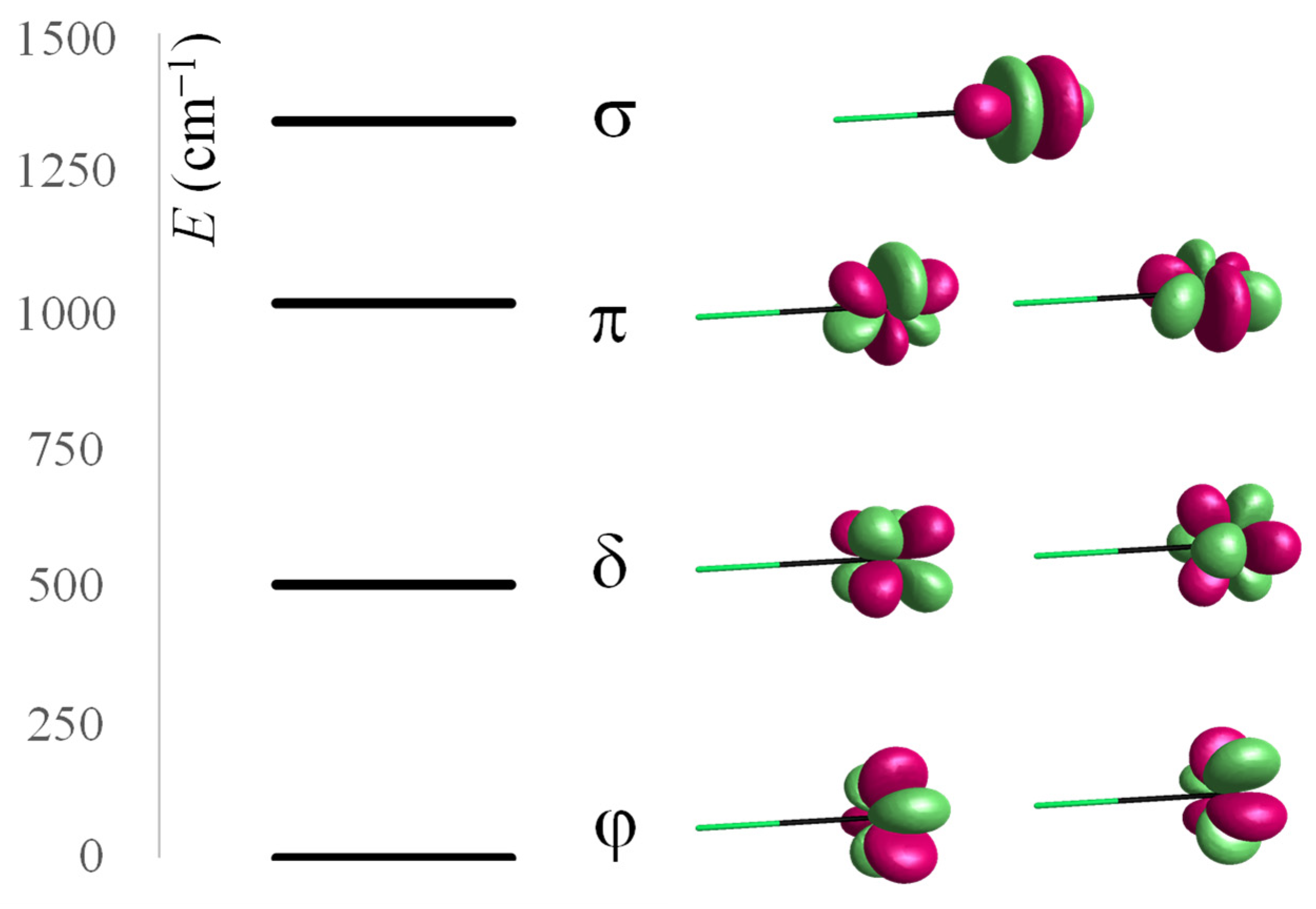
Let us consider some Tb(III)-based model systems in CASSCF calculations, including eight electrons in seven orbitals, CASSCF(8,7). [TbF]+2 does not correspond to any experimentally known species but offers a first glance into LF parameterization. The Tb–F distance is conventionally set to 2.35 Å, corresponding to the range encountered in various solid-state fluorides [68,69,70]. The CASSCF-computed states assignable to the 7Φ, 7Δ, 7Π, and 7Σ spectral terms, ordered in this sequence, have the relative energies 0.0, 497.5, 1008.7, and 1339.8 cm−1, respectively. Figure 1 depicts the computed levels and suggests the relationship with the orbital LF scheme, depicting the canonical MOs, which is practically almost pure AOs, which can be described as the location of the β electron for the given spectral term. In this simple case, the terms are parallel to the itinerant fβ component from the f8 ≡ f7αfβ configuration of Tb(III). The scheme also suggests the meaning of the AOM-type parameterization, namely, the relative magnitudes of the efσ, efπ, and efδ perturbations for f electrons, after conventionally setting the efφ = 0 energy origin. The above energy levels were obtained in the primary active space of CASSCF(8,7), related to the f8 configuration. Extending the space to also comprise the five d-type virtual orbitals to CASSCF(8,12), the split of 7F term is slightly modified, with the results being interpreted as the following AOM parameters: efσ(F) = 1175.0 cm−1, efπ(F) = 910.2 cm−1, and efδ(F) = 466.5 cm−1, in addition to the imposed efφ = 0.
Note that the eδ parameter is not negligible, as customary in the established AOM practice, presuming efδ and efφ are null, because the ligands are not expected to be able to exert δ and φ true orbitals overlap. Let us ignore this apparent discrepancy for the moment, debating the available details of the proposed computational experiments.
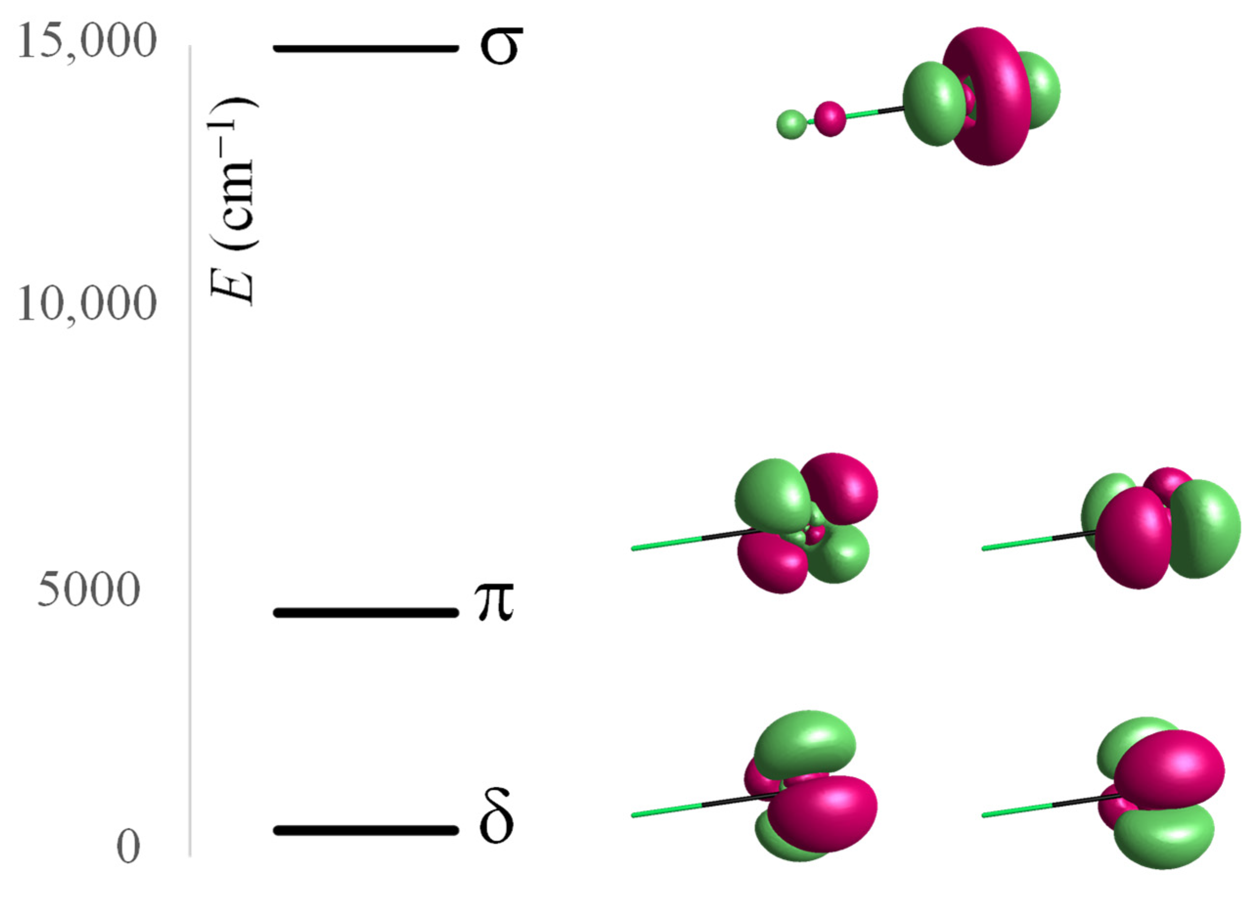
The Tb(III) ion is also well suited to discuss the d-type ligand field in lanthanides, analyzing the f8 → f7d orbital promotions (implying 5d empty AOs) in the CASSCF(8,12) setting. The f7 subconfiguration is spherically symmetric, the set of f7d excited states then has D representation, and the spectrum is parallel with the LF scheme of d electrons. In more detail, there is a 7D term arising from the f7αdβ configuration and a 9D term arising from the spin swap to f7αdα. The high-spin states are lower in energy, benefiting from stabilization by the f–d inter-hell exchange coupling. In the following, as a measure of the d-type LF split, we consider the spin-septet terms, keeping the same multiplicity as in the 7F ground state. To be distinguished from the d-type LF encountered in transition metal complexes, here, we deal with an excited-state d orbital population. In linear symmetry, the 7D term splits into 7Δ, 7Π, and 7Σ levels. Shifting the 7Δ orbital doublet to zero, namely, imposing edδ = 0, the relative gaps can be assigned to the d-type AOM parameters, resulting in edσ(F) = 14,959.7 cm−1 and edπ(F) = 4518.9 cm−1. Figure 2 shows the discussed spectral terms and the assigned d-type orbitals from the f7d orbital promotions. In debating the effective one-electron parameters, the overall shift in the 7Δ is ignored because it is due to non-LF effects. As expected, the d-type LF split is sensibly larger than the f-type LF split because, having a larger radial extension, the 5d orbitals are closer to the ligand sites, undergoing a larger perturbation.
Considering that an LF scheme has the meaning of orbital energies in a given environment, there is a naïve expectation that computed canonical orbital levels may directly provide this scheme. Strictly speaking, this is not generally true, and is particularly not expected in the case of CASSCF techniques, where the orbitals are merely intermediate objects used to set the many-electron problem, their energies being subject to certain conventions (MO canonicalization [27]). However, we can verify that, in our case, the relative energies of f-type optimized orbitals, corresponding to φ, δ, π, and σ labels, {0.0, 482.8, 987.6, 1448.5} cm−1, parallel the computed gaps between the 7Φ, 7Δ, 7Π, and 7Σ spectral terms. This regularity also occurs with respect to the d-type sequence, with the corresponding molecular orbitals having relative energy gaps similar to those of the D spectral terms: {0.0, 5464.9, 14,704.8} cm−1. Recall that in the axial symmetry, the σ or Σ labels correspond to nondegenerate states, while the other ones represent doubly degenerate couples.
After conducting a thorough investigation on the grounds of simplified systems, we now consider the artificial [TbNe]+3 molecule to produce a measure of LF perturbation in the absence of charge. The neon atom is roughly similar as an electronic structure to the structure of a fluoride anion. The AOM parameters extracted from computed 7F spectral terms are efσ(Ne) = 264.5 cm−1, efπ(Ne) = 148.1 cm−1, and efδ(Ne) = 66.5 cm−1, with imposed efφ = 0.0; those of the 7D origin are edσ(Ne) = 2342.9 cm−1, edπ(Ne) = 661.3 cm−1 while setting edδ(Ne) = 0.0. The values are sensibly smaller than those of the fluoride ligand, indicating, in a semiquantitative sense, the important contribution of the electrostatic part.
We next considered linear [TbF2]+ in the next computer experiment, observing similar spectral terms, because the molecule now spans the D∞h symmetry, having the previous C∞v of the asymmetric linear molecule as a subgroup. Then, for the same series of spectral terms, 7Φ, 7Δ, 7Π, and 7Σ, from the atomic 7F state, the calculation produces the 0.0, 1044.5 cm−1, 2109.1 cm−1, and 2926.9 cm−1 gaps, namely, about double values, in comparison with those of [TbF]+2. In this way, for f electrons, we reasonably retrieved the additivity hypothesis intrinsic to LF models. For the d shell, the split in [TbF2]+ is 0.0, 7764.5 cm−1 and 15,033.9 cm−1 for 7Δ, 7Π, and 7Σ. Then, quite intriguingly, when the π-type perturbation in [TbF2]+ is roughly twice that in [TbF]+2, the d-type σ perturbations are similar in [TbF]+2 and [TbF2]+. We suppose that because of the stronger interaction between the 5d shell and the ligand, the simple premises of LF are not strictly followed, particularly not in the σ overlap, achieving an advanced intercept of the ligand near the maximum 5d radial zone. As in the previous case, the relative f-type orbital energies are quite similar to the spectral terms: {0.0, 1031.5, 2041.1, and 3006.8} cm−1 for the {φ, δ, π, and σ} sequence of f-type orbitals, respectively. In turn, the orbital energies are not a good measure for the d-based LF sequence, with the relative values for {δ, π, and σ} being {0.0, 9986.1, and 20,455.0} cm−1, respectively.
Given the good parallelism between the spectral terms corresponding to the f-based LF scheme and f-type orbital energies, we may suggest that these can be taken as approximations in situations where the relationship with the spectral term energies is not simply defined. Thus, for a Gd(III) free ion, having a nondegenerate 8S ground state, with the higher spectral terms being only spin sextets, the {φ, δ, π, and σ} relative orbital energies in [GdF]+2 are {0.0, 482.8, 943.7, and 1316.8} cm−1, respectively, quite similar to those of the [TbF]+2 case. The same regularities hold for [GdF2]+, which has {0.0, 1009.6, 1997.2, and 2875.1} cm−1 f-type orbital gaps, approximately double the values of the single-ligand model molecule.
The following numeric experiment demonstrates the variation in the computed spectral terms in the [TbF2]+ unit as function of the F–Tb–F angle, which we performed to check whether the geometry dependence follows the pattern of the angular overlap model version of ligand field theory. Figure 3a shows the computation data with open circles and the fitted AOM variation with a continuous line. The adjusted parameters, accounting for the whole variation, are efσ(F) = 1341.7 cm−1, efπ(F) = 1018.6 cm−1, and efδ(F) = 514.3 cm−1. The CASSCF and AOM data were fitted in their barycenters for better visualization. The fit is quite good in the 90°–180° domain of the F–Tb–F angles, with the deviation at lower angles being pardonable because it enforces the strong ligand–ligand repulsion, and the small inter-ligand angles are avoided in real lanthanide chemistry. The conclusion that the AOM pattern is satisfactorily obtained with the calculation also holds for the d-type LF, represented in Figure 3b. The parameters giving an overall satisfactory fit to the d-LF angular variation are edσ(F) = 8356.6 cm−1 and edπ(F) = 3690.5 cm−1, with a constrained edδ(F) = 0.0.
Imposing F–Tb–F = 90° allows us to debate a subtle issue of ligand field models. One may observe that, at this point, two pairs of emulated AOM states are crossing, as if degeneracies are occurring. The TbF2+ unit has C2v symmetry in all geometries when it is nonlinear, not admitting degenerate states. Indeed, the computed points are not superposed in a state-crossing situation, although the corresponding pairs of values are mutually close. In this situation, we observe a hidden feature of LF models, called holohedrization. The term was coined by Schäffer [71,72], being a definite feature of LF models, but it is largely ignored in common practice. It arises because the expansion of LF potential in Equation (1) is based only on even spherical harmonics, k = 2, 4, and 6, in the case of an f shell. Thus, it cannot account for asymmetric LF maps. In other words, this creates, for every perturbation coming from a given ligand, a ghost image at its antipode. Then, the perturbation of a ligand L is actually divided into two halves, one generated from its real position, say at {xL, yL, zL} Cartesian coordinates; and another from the {−xL, −yL, −zL} inverted point. This artificial effect of LF models is tacitly inherited in AOM too. Then, in AOM as well, the perturbation due to the Tb–F contact is smeared as if produced by two-halves of fluorine ions in diametrically opposed placement, (F/2)–Tb–(F/2). By the same reason, a [TbF2]+ unit with F–Tb–F = 90° behaves as a square of four ligand halves. Therefore, the LF potential and AOM matrix artificially acquire the D4h symmetry of the square, where the representation of the f orbitals is a2u + b1u + b2u + 2eu. The two doubly degenerate eu elements are the crossing points described in the above discussion. The d-type LF scheme, shown in Figure 3b, shows a single crossing due to holohedrization, because the representation of d orbitals in D4h, a1g + b1g + b2g + eg, contains one doubly degenerate component.
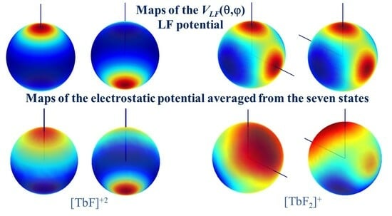
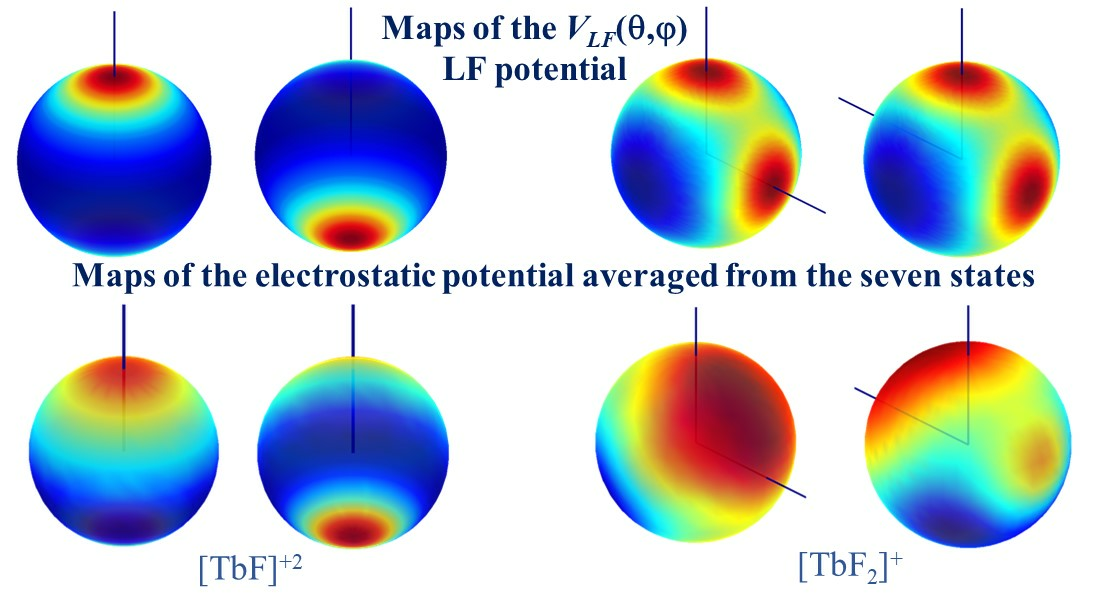
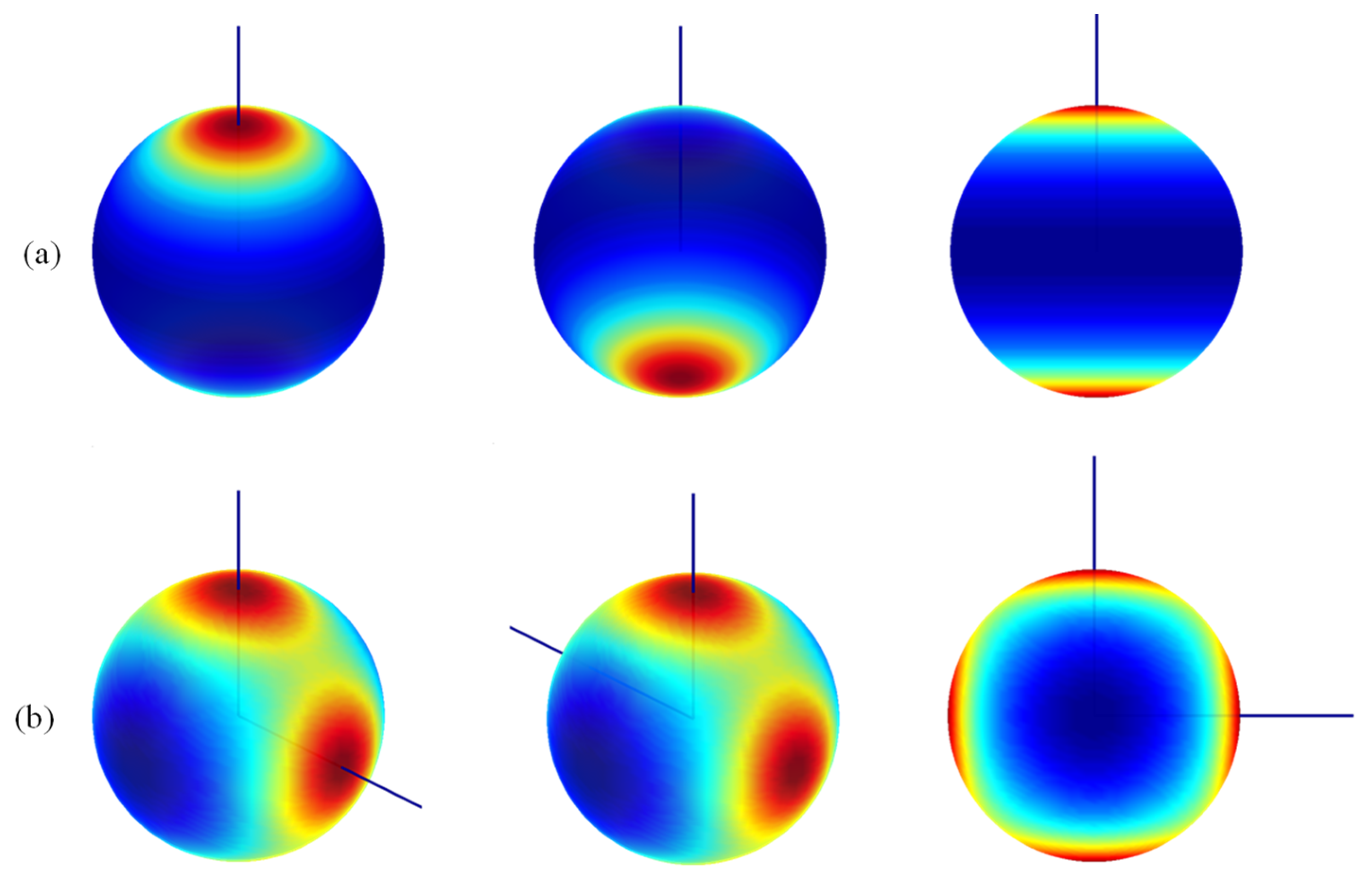
An illustration of the holohedrization is represented using the color map of Equation (1). If the θ and φ variables are drawn as the parallels and meridians of a sphere, the variation in the VLF(θ, φ) potential is qualitatively suggested by the color shading, taking deep blue for the lowest values, purple-red for maxima, and the orange-yellow-green palette for the in-between range. The sphere is taken on an arbitrary scale with respect to the molecular skeleton.
One can observe in Figure 4 that the action of the ligand is mirrored at its inversion center. For instance, in panel 4a, the ligand is placed at the north pole, but the caps of red coloring, marking the positive perturbation from the negative ligand against the negative electrons, show an equal size at the south pole. With the same factor and the holohedrization effect, the LF potential of the angular [TbF2]+ unit at F–Tb–F = 90° has four-fold symmetry. The actual C2v symmetry of the system has an artificial inversion center, generally becoming D2h and particularly D4h at the rectangular geometry. The artificial-square-like symmetry is clearly seen in the inset in the right-bottom corner.
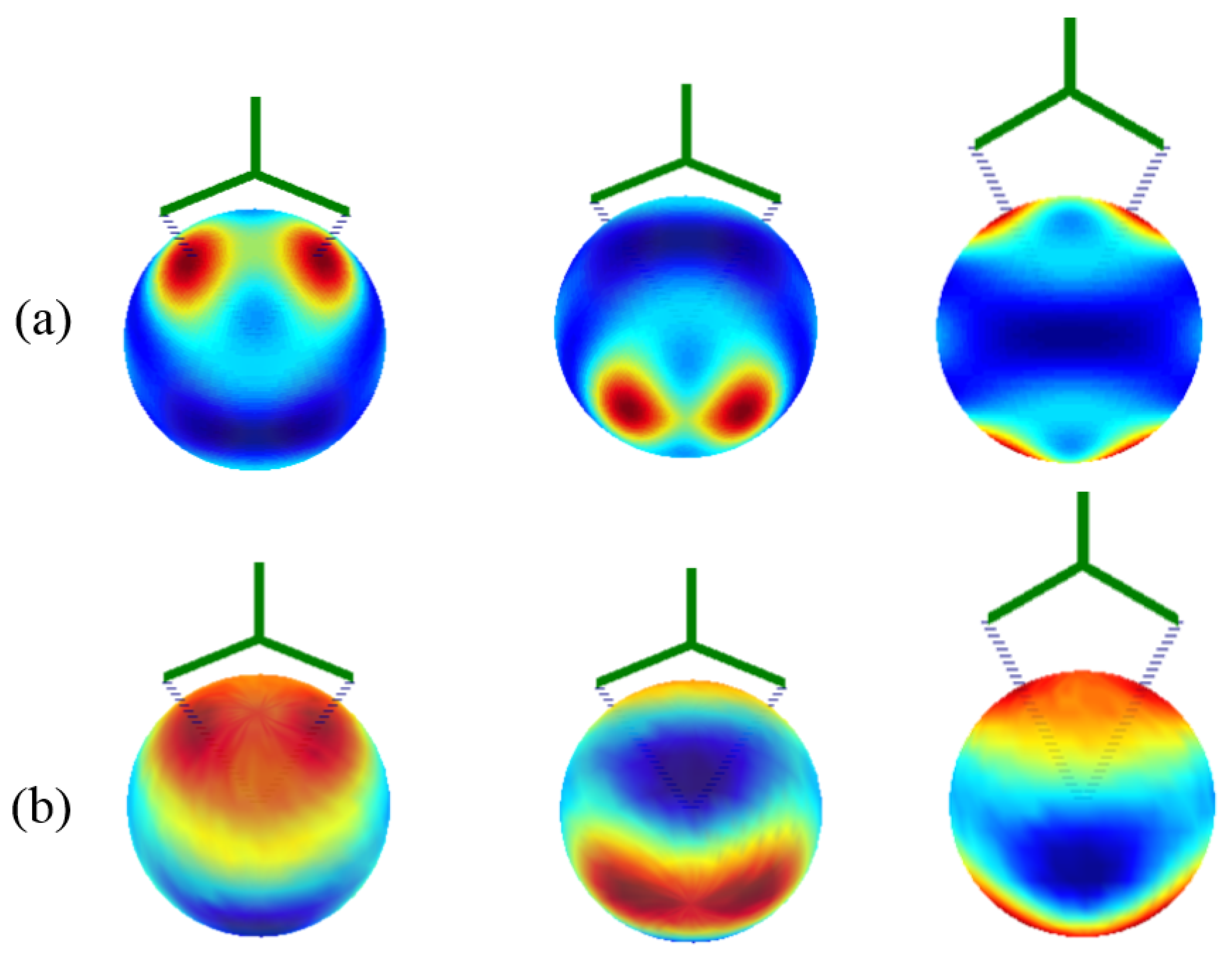
In this intriguing situation, we proceeded to the examination of the ab initio computed electrostatic potential. Figure 5 shows the same systems with electrostatic potential drawn on a sphere with radius 0.5 Bohr, corresponding to the maximum of the radial profile of the f shell in the given atomic basis. To improve visibility, the spheres represented here are scaled in arbitrary mode. In more detail, we rendered the averaged electrostatic potential collected from the seven states of the state-averaged CASSCF calculations of the discussed systems.
In the upper half of Figure 5, somewhat surprisingly, a map suggesting the partial subsistence of the holohedrization effect appears in the case of the [TbF]+2 diatomic molecule. A red area marking the axial penetration of the LF perturbation at the antipode of the Tb-F bond is clearly visible but is smaller than those appearing under the ligand. The map of [TbF2]+ in the lower half of Figure 5 more substantially differs from the emulated LF map in Figure 4, showing only small spots at the antipodes of the Tb-F bonds and an absolute maximum between ligands along the line bisecting the F–Tb–F angle.
We may conclude that the holohedrization, although due to the limitations of the LF models is in part a true phenomenon for the f-shell compounds. This is an important result of this work, with the issue deserving further debate. As previously noted, holohedrization is largely overlooked in the current LF practices. Graphical LF mapping, as we show here, has not been exploited despite the relevance of this issue.
We could not check the above-discussed LF quantities against experimental data, because the selected case studies are artificial, given our aim of extreme simplicity to obtain academic insight. However, one may attempt a step toward more realistic objects considering the octahedral [TbF6]−3 unit. As a stand-alone molecule, this molecule is not fully realistic, but similar units can be found as doped sites in elpasolites [73,74,75].
The AOM equates the octahedral LF eigenvalues as follows:
Inserting previously ascribed the efλ(F) values from the CASSCF(8,12) calculation on [TbF]+2, we predicted values of 916.3 cm−1 and 409.5 cm−1 for the and gaps, respectively. The calculation of the [TbF6]−3 unit, in settings similar to those of the diatomic metal–ligand system, gives Δ1 = 762.9 cm−1 and Δ2 = 291.9 cm−1, which are roughly comparable to the result assuming the transferability of the AOM parameters. The discrepancy is explained by the different balances in the non-LF effects subsisting in the positively charged artificial diatomic system versus the negatively charged larger system. The AOM practice does not consider the octahedral gaps with the full set of {eσ, eπ, eδ, eφ} parameters, being confined only to the {eσ, eπ} couple, first by the empirical assumption that the effects of δ and φ are not chemically intuitive and then by the pragmatic reason that the available data do not allow obtaining a full parametric scheme. Thus, if we consider that the two gaps for the [TbF6]−3 unit are fitted only in the σ-π scheme, we obtain eσ = 293.9 cm−1 and eπ = 116.7 cm−1, which is in a range compatible with the experimental spectroscopy [42,76]. Although the chemical intuition may refute the φ and δ bonding effects, the electrostatics support their underground action. However, we leave this matter as a challenge open to further debate. We honestly admit that the calculations have certain limitations; from a different perspective, they can offer more details than are available from experiments.
Let us now take a polyatomic ligand, maintaining the simplicity; a relevant case study is the nitrate coordinated in chelate symmetric mode. The Tb-O distances are conventionally imposed at 2.35 Å. The CASSCF calculation results in the full split of the 7F term into seven distinct levels (though with very small spacing between first and second states) with the following relative energies: 0.0, 1.7, 451.1, 488.8, 499.6, 765.0, and 1184.5 cm−1. Via the handling of the Hamiltonian matrix of the CASSCF calculations, these values are fitted by the parameters from Equation (1), as follows: = 1410.8 cm−1, = −203.2 cm−1, = −465.9 cm−1, = 179.4 cm−1, = 376.6 cm−1, = 885.5 cm−1, = 44.3 cm−1, = −19.5 cm−1, and = −1.9 cm−1. We observe that in the given symmetry, only parameters with non-negative and even q indices do not vanish.
The determination of the parameters enabled the drawing of the VLF(θ, φ) ligand field potential map, shown in the upper part in Figure 6. The LF maps undergo holohedrization, with the two maxima due to coordinated oxygen atoms being reflected exactly at the opposite pole. Interestingly, holohedrization is also visible in the ab initio electrostatic potential, averaged over the seven CASSCF states, as illustrated in the bottom half in Figure 6. The potential contours under the ligand and those recorded at antipodes are not perfectly similar but are comparable, again emphasizing that the identification of holohedrization in this numeric experiment is a nontrivial finding.
The previously outlined parameters are not transparent in their physical meaning. To attempt a more intuitive interpretation, we considered the AOM scheme. Here, the classical AOM knowledge indicates a limited set of parameters. One efσ(O) is assignable to the lone-pair oriented toward the metal, with the π effects dichotomized in one due to the nominal π orbitals, with lobes perpendicular to the ligand plane efπ⊥(O), and another acting in plane efπ||(O), which may be negligible. The two oxygen atoms are equivalent, receiving equivalent parametric definitions.
Judging by the degrees of freedom available in the given C2v symmetry, the parametric leverage proposed by intuition-driven AOM is too constrained, having three variables, while the approach in Equation (1) produces nine adjustable terms. To verify the available degrees of freedom, we counted the repetitions of the A1-irreducible component in the representation of k = 2, 4, and 6 sets of spherical harmonics in C2v. Thus, we picked two from k = 2 (2A1 + A2 + B1 + B2), three from k = 4 (3A1 + 2A2 + 2B1 + 2B2), and four from k = 6 (4A1 + 3A2 + 3B1 + 3B2), acquiring the nine-dimensional parametric variance.
The attempt to fit the simplest AOM scheme gives parameters that seem acceptable: efσ(O) = 835.2 cm−1, efπ⊥(O) = 438.4 cm−1, and efπ||(O) = 264.0 cm−1 (the in-plane π was not vanishing, as hoped) and a sequence of LF energies {0, 14.5, 352.4, 369.3, 507.4, 650.38, 1181.2} cm−1, which very roughly reproduce the computed values. Allowing more parameters, such as efδ⊥(O), efδ||(O), efφ⊥(O), and efφ||(O), improves the match of the LF spectrum (although it does not make it perfect) at the cost of nonvanishing values for these terms, which do not belong to the classical canon of the AOM.
3.2. Density Functional Account of Ligand Field Problems
In the following, as case studies, we use the same objects as in the previous section, devoted to multiconfigurational calculations. Because the fn configurations, except the f7, have degenerate ground states, and their compounds (within the expected weak LF) are quasidegenerate systems, DFT should not be applied without special caution and wise techniques. Considered in an unrestricted self-consistent version, i.e., allowing different molecular orbitals for α and β spins, one may obtain convergent solutions, which should be considered with precaution [46]. Unrestricted calculations are not well-suited because the energies of the f-type orbitals may drastically differ in α versus β series, which is a situation incompatible with the LF paradigm. On the other hand, restricted-type DFT calculations are prone to severe convergence problems, a situation that can be described as due to the non-Aufbau configuration of lanthanide ions in compounds [37]. As illustrated, we briefly mention the unrestricted DFT attempt (with BLYP functional) of the [TbF]+2 system in the same GAMESS code used for the previous CASSCF calculations. The simplest unrestricted calculation with no educated guess does not reach convergence. Inserting a guess provided by the CASSCF calculation (with the same MOs initially doubled for the α and β sets), we obtained a convergent solution containing seven f-type α functions in the range −0.902 to −0.857 Hartrees, i.e., with a gap of 9690 cm−1, which is too large for the LF scale. There are two β f-type orbitals instead of the expected one fβ component, whose energies, at −0.770 and −0.777 Hartree, are very distant from the range of fα orbitals by about 29,000 cm−1. The restricted calculation attempt was a total failure. It is clear then that the brute-force DFT approach is not satisfactory.
In order to assess the density functional theory (DFT) approach to LF, we employed the Amsterdam density functional (ADF) code [59,60], which allows a rather wide range of computational experiments based on the control of orbital populations, a feature usually not available in many codes.
The advanced ADF controls allow restricted-type calculations, enforcing fractional occupation with 8/7~1.1428 on each of the seven f-type orbitals expected to emulate the LF sequence. It is important to note that fractional occupations are conceptually allowed in DFT [77,78] and are technically enabled in the ADF environment. Averaging the population of the fn configuration to n/7 for each f-type orbital, we can overcome the ban on using DFT for quasidegenerate ground states. Taking the concrete case of Tb(III) with an f8 configuration, where we must have a doubly occupied f-type orbital, it is expected that, in principle, small energy differences occur if different configurations are prepared with the doubly occupied MO moving along the seven f-type orbitals; this is outside the validity of DFT according to its basic theorems [79]. If, in turn, the content of the double-occupied orbital is smeared on the components of the LF-type set, this dilemma disappears because we consider an object having a singly defined, though artificially devised, state. From another perspective, the orbital averaged scheme is somewhat similar to the state-averaged calculations performed in multiconfigurational mode.
The population control in ADF is also helped by symmetry, making it possible to organize the orbitals by their point-group representation. Thus, in the C∞v symmetry of the [TbF]+2 molecule, there is a core due to the [Xe] and [Ne] configurations of the inner Tb(III) shells and fluoride anion, with occupation [Xe-Ne] = σ28π28δ8. The LF part has the fractional populations φ16/7δ16/7π16/7σ8/7.
We took the orbital energies of the restricted calculation with this definition, and we interpreted the gaps as akin to f-type AOM parameters, with efφ = 0 fixed at zero. The results are shown in the first row in Table 1. In comparison with the results from CASSCF, it seems that this computational setting overestimates the LF parameters. We can explain this by the slightly faulted description of the f characteristic in the MOs determining the LF sequence. In the multiconfigurational calculations from the previous section, the canonical orbitals were obtained with almost 100% content in f AOs; in the above-described DFT calculation, this happens only for the δ and φ orbitals. The π functions were obtained with only 74% f and the σ with about 89% f, with the remainder being due to the ligand. This creates a nonphysical asymmetry in the shape of the f-type components, leading to the overestimation of the LF parameters. On the other hand, although improperly balanced, we comment that this situation is in the spirit of AOM, i.e., driven by weak covalency occurring on σ and π channels but not on the δ and φ components.
Here, we comment on the expected dependence on the choice of the density functional. For instance, conducting the calculation with the B3LYP hybrid form, we obtain efσ(F) = 6121.9 cm−1, efπ(F) = 1645.4 cm−1, and efδ(F) = 3008.5 cm−1, noticing a nonphysical swap of π vs. δ orbital energies.
The leverages of the ADF code allow the emulation of excited orbital configurations. In the following numeric experiments, the doubly occupied MO from the f8 configuration was successively placed in different LF-type orbitals, i.e., among functions with a preponderant f characteristic. The orbitals were kept frozen as a result of the above-discussed averaged-population result. The second line in Table 1 lists the total energy of the φ3δ2π2σ1 configuration as zero of the energy scale, with the relative energies of the φ2δ3π2σ1, φ2δ2π3σ1 and φ2δ2π2σ2 states assimilated to the efδ, efπ and efσ perturbations, respectively. As such, we break the rule that DFT is not enabled for excited states. However, in this particular case, we may invoke a symmetry-sustained dispense. The above-outlined configurations span different representations of their Slater determinants, 7Φ, 7Δ, 7Π, and 7Σ. Then, we state that each configuration acts as a ground state on the different symmetry channels, providing validity to the population-controlled calculation in the DFT frame. The numeric values do not well reflect the expected LF pattern. The negative efδ(F) means that φ2δ2π3σ1 is a ground configuration, instead of the initial expectation of a φ2δ3π2σ1 configuration. Although this numeric experiment is, in principle, more advanced than the assimilation of orbital energies with the LF diagram, it did not lead to an actual improvement. The third line in Table 1 illustrates a tentative refinement by taking iterative calculations on the tuned configurations, with the results remaining unsatisfactory.
The fourth line in Table 1 addresses a specialized handling implemented in ADF, called frozen density embedding (FDE) [80,81]. Although not specifically aimed at ligand field problems, the FDE approach serves this idea well because, in our case, the calculation is performed only on the electrons of the metal ion, with the ligand counting only as surrounding electron density. The approach is not confined only to the classical electrostatic field because it also accounts for the exchange and kinetic energy effects from the frozen electronic cloud of the ligands, taken as fragments described in the preamble from free anions. The FDE-DFT calculation is then performed only on the Tb(III) ion, selecting the energies of the perturbed f orbitals. The frozen ligand density result seems to be in the correct range, being close to the CASSCF data reported in the previous section.
In the following, we discuss the results obtained in unrestricted mode. Now, population averaging occurs only for one electron in β-type orbitals, while the α f-type orbitals are filled with seven electrons, i.e., [φ2αδ2απ2ασα] φ2β/7δ2β/7π2β/7σβ/7, corresponding to the f7αfβ/7 formulation of the f8 configuration of Tb(III). In this case, we selected two series of orbital energies for the two spin polarizations. We remark on the persistence of parametric overestimations and on a strange swap of efσ vs. efπ ordering for the α-type orbitals. The numeric experiments with the imposed orbital occupation schemes considered the following configurations: [φ2αδ2απ2ασα]φβ, [φ2αδ2απ2ασα]δβ, [φ2αδ2απ2ασα]πβ, and [φ2αδ2απ2ασα]σβ, with the energy of the first taken as a relative reference. The results of the configurations for the frozen MOs were catastrophic; it is hard to explain why. However, the results improved if orbital iterations were allowed for each configuration, with a quite good eσ but poor eπ and eδ values. The unrestricted FDE approach must consider two sets of orbital energies. As in the restricted version, this technique, which is an approximation, yields a result compatible with that of the LF paradigm. Particularly, the FDE β-type efλ parameters show a resemblance to the CASSCF results.
Table 2 shows the results of the same series of calculations applied to the linear [TbF2]+ molecule. In this case, all computed energy gaps were divided by two with the idea of obtaining LF perturbations assignable to one fluoride ligand.
In the [TbF2]+ system, although a general overestimation of LF parameters occurs, it has a smaller amplitude than that of the [TbF]+2 system (except for the well-behaved FDE estimation). We tentatively explain this by the symmetric characteristic due to the F–Tb–F axis. Although this does not reduce the overestimated metal–ligand mixing, the orbital shapes with inversion symmetry better account for the effective LF phenomenology than the polarized bonds along the diatomic Tb–F line.
Let us briefly examine the DFT results on the [TbF6]−3 unit that were obtained using the symmetry and occupation keywords. The energies of the restricted f-type MOs with eight electrons smeared on the seven orbitals spanning the a2u + t1u + t2u composition gave gaps of Δ1 = 1855.1 cm−1 and Δ2 = 709.8 cm−1 (see notations for Equations (4)–(6)), which were about twice larger than those produced with the CASSCF estimation. The unrestricted calculation is puzzling, yielding spurious results for α-type MOs of Δ1 = −2242.3 cm−1 and Δ2 = −685.6 cm−1, while producing semiquantitatively acceptable results for β-type MOs of Δ1 = 1371.2 cm−1 and Δ2 = 524.3 cm−1. Connecting the points, it seems that DFT generally overestimates the LF perturbations, which is curiously attenuated in larger systems: severe in [TbF]+2, large in [TbF2]+, and partly acceptable in [TbF6]−3. This can be understood by the fact that in larger systems, the central ion feels an averaged field closer to the quasispherical situation in which the LF paradigm is constructed. The quantitative lapses in the smaller systems deserve, however, to be kept under observation, signaling an unbalanced interplay of factors inside the black box of DFT computation. As a conclusion, we state the caveat about the general problems with DFT in describing the LF parameters, emphasizing however, the reliability of the FDE approach, at least for the situation of the f shell in ionic lanthanide complexes.
3.3. Revisiting the Crystal Field Electrostatic Approximation
Let us now consider the calculation results with standard LF Hamiltonian from Equation (1), taking the simplest case of the [TbF]+2 model molecule, as described in Section 3.1. As outlined in the Introduction, Equation (1) should obey the symmetry of the problem, taking the combinations of the spherical harmonics that render total symmetric representation in the given point group. In the case of linear systems, such as [TbF]+2, in the C∞v point group, the total symmetric representations are simply the Yk,0 components in each spherical harmonic set. In other words, only the parameters are retained, and all the other ones, with q ≠ 0, vanish. The ab initio results on [TbF]+2 from Section 3.1 were fitted with = 2037.7 cm−1, = 662.3 cm−1, and = 232.4 cm−1. According to convention, the eigenvalues are placed with their barycenter in the zero of the energy scale. If we add an overall shift, with = 386.9 cm−1, the eigenvalues are the same as interpreted in the AOM parameterization, with a fixed eφ = 0.0 cm−1. We here relabel the parameters . For the one-ligand case, in the C∞v point group, the eigenvalues of the Hamiltonian from Equations (1) and (2) in terms of parameters, classified by (σ, π, δ, ϕ) symmetry labels, are:
Note that the sum of the eigenvalues is , with the standard LF scheme imposing b0 = 0. In the AOM, we postulate or, equivalently, .
If the LF Hamiltonian is taken in the crudest electrostatic definition, determined by a qL point charge at distance RL from the lanthanide center, the bk parameters are
where r is the radial coordinate of the electron, and R(r) is the radial function of the atomic orbitals undergoing the LF perturbation. This expression comes from the multipolar expansion of the electrostatic potential [1,2]. Although it quickly became clear that this estimation was not working, tacitly referring to the d-type LF frame, we revisited this issue because, to the best of our knowledge, it has not been re-examined in the modern age of computation with a focus on the lanthanides case.
The evaluations with the above equation do not depend on a dedicated calculation method: they are determined merely by the basis set of the LF shell. Because we worked in the Gaussian-type orbital (GTO) based frame in Section 3.1 and we used a Slater-type orbital (STO) set, specific to the ADF infrastructure, in Section 3.2, we exploited the opportunity to check the idea of first-principles electrostatic approximation using these different definitions.
The radial part of the LF shell is taken as a linear combination:
where ni and ζi are the power and exponent parameters of the primitive χ functions defining the basis, respectively; ci are the coefficients resulting from the self-consistent calculation; and Ni are the normalization factors.
In the GTO case, the primitives are
with the normalization factors
expressed in terms of the gamma incomplete function.
In the STO frame, the primitives and normalization factors are:
In both cases, the general formulation of the pure electrostatic LF parameters is:
The Pij and Qij terms have specific expansions in GTO vs. STO instances. With the help of MathematicaTM [63,64] computer-algebra code, we were able to derive closed analytical formulas, being close in the GTO case:
For STO, we obtained:
Let us apply the GTO formulas for the free Tb(III) ion, taken on the SARC-ZORA basis [82] with a ζ = {32.1811, 10.727, 3.57568, 1.19189, 0.397298, 0.132433} sequence of exponent parameters in Bohr−2 units, and all ni = 4. The state-averaged CASSCF calculation on the 7F ground state defines the set of c= {0.405816, 0.614349, 0.227727, −0.0382306} coefficients. Inserting these values into the above formulas, we obtain electrostatic parameters b0 = 49,464.5 cm−1, b2 = 1964.1 cm−1, b4 = 189.2 cm−1, and b6= 49.7 cm−1, which determine the relative eigenvalues eσ = 1207.8 cm−1, eπ = 1028 cm−1, eδ = 601.4 cm−1, and eφ = 0 (equivalent to the AOM definitions), respectively. The b0 parameter, usually ignored in the LF expansion, is very close to the classic point-charge potential, 1/RL = 0.225182 a.u. ≡ 49,421.7 cm−1. The bk parameters are in the same range as those fitted from the ab initio spectral terms, but they do not match perfectly. On the other hand, the relative eigenvalues are very similar in the two schemes.
In the following, we check the pure electrostatic approximation of the LF parameters for the STO-type ZORA/TZ2P basis used in the calculations in Section 3.2. This basis is defined by ζ = {10.2, 4.9, 2.15, 1.65} exponent parameters in Bohr−1 and the n = {4,4,4,5} sequence of power factors. The BLYP calculation of the free Tb(III) ion provides c = {0.405816, 0.614349, 0.227727, −0.0382306} coefficients. The STO-based estimation yields b0 = 49,421.5 cm−1, b2 = 2257.0 cm−1, b4 = 271.2 cm−1, and b6 = 67.3 cm−1, which are just a bit larger than the results from GTO. With this, we derive the following parameters: eσ = 1395.3 cm−1, eπ = 1176.3 cm−1, and eδ = 675.64 cm−1 if conventionally considering eφ = 0. The results are fully comparable to those for GTO.
We obtained, via the crudest crystal field approximation, results that are compatible with those of high-level multiconfigurational calculations. This contradicts the long-standing belief about the failure of pure electrostatic estimation. Actually, the description of pure electrostatic paradigm was pronounced about d-type LF systems, where partial covalent bonds truly occur in coordination compounds. Sed contra, lanthanide compounds are more ionic and are therefore better suited for the original ideas of electrostatic ligand fields. This situation deserves further debate; here, the limitation is that the results may be due to the very simplified nature of the discussed cases, with the imposed idealization having yet insightful value and even practical connotations, suggesting that if proven that we can rely on a simpler level of approximation in applications.
4. Conclusions
We performed an unprecedented examination of the computational methods used for the LF-dedicated description. The deliberate use of extremely idealized case studies produced details usually hidden in calculations on large-scale systems, which deserve to be considered in further explorations and exploitations of current practical problems.
Comparing the methods pertaining to wave function theory (WFT) versus those of density functional theory (DFT), we clearly concluded that the former is better suited for LF problems, while adapting the rather unsystematic DFT to this aim may be a useful quest.
Strikingly, revisiting the early hypothesis of the electrostatic nature of LF perturbation, we found it suited for the ionic complexes of lanthanides. We produced very similar LF parameters using crude estimations with the point-charge perturbation of the atomic f shell via multiconfigurational WFT methods and by the DFT, confined to the frozen density embedding (FDE) approximation. These corroborated results hint at the possible design of simplified approaches that are usable in complicated situations, specific to property-design challenges in the search for new materials. Here, LF can be a valuable ancillary tool in luminescence problems.
Here, we confined our study to hard-base ionic ligands. The conclusions are valid as extrapolation for large classes of solid-state systems with such characteristics (e.g., fluorides, oxides, phosphates, and silicates). We acknowledge that the factors may change if we consider systems in the opposed extreme, i.e., neutral and soft-base ligands, creating a challenge open to debate for the outlined issues.
Author Contributions
Conceptualization, A.M.T. and M.C.B.; software, B.F.; validation, A.M.T., B.F., C.I.O. and M.C.B.; formal analysis and investigation, A.M.T., B.F., C.I.O. and M.C.B.; resources, A.M.T. and M.C.B.; data curation, A.M.T., B.F., C.I.O. and M.C.B.; writing—original draft preparation, A.M.T. and M.C.B.; writing—review and editing, B.F. and C.I.O. All authors have read and agreed to the published version of the manuscript.
Funding
This research was funded by the National Romanian Office for Research, UEFISCDI, grant No. PN-III-P4-PCE-2021-1881, contract No. 123/2022.
Data Availability Statement
Details are available from the corresponding authors.
Conflicts of Interest
The authors declare no conflict of interest.
References
- Ballhausen, C.J. Introduction to Ligand Field Theory; McGraw-Hill Book Co.: New York, NY, USA, 1962. [Google Scholar]
- Newman, D.J.; Ng, B.K.C. Crystal Field Handbook; Cambridge University Press: Cambridge, UK, 2000. [Google Scholar]
- Bethe, H. Termaufspaltung in Kristallen. Ann. Der Phys. 1929, 395, 133–208. [Google Scholar] [CrossRef]
- Van Vleck, J.H. Theory of the variations in paramagnetic anisotropy among different salts of the iron group. Phys. Rev. 1932, 41, 208–215. [Google Scholar] [CrossRef]
- Solomon, E.I.; Lever, A.B.P. Inorganic Electronic Structure and Spectroscopy: Methodology Volume I Edition; Wiley-Interscience: New York, NY, USA, 1999. [Google Scholar]
- Singh, S.K.; Eng, J.; Atanasov, M.; Neese, F. Covalency and chemical bonding in transition metal complexes: An ab initio based ligand field perspective. Coord. Chem. Rev. 2017, 344, 2–25. [Google Scholar] [CrossRef]
- Zadrozny, J.M.; Xiao, D.J.; Atanasov, M.; Long, G.J.; Grandjean, F.; Neese, F.; Long, J.R. Magnetic blocking in a linear iron(I) complex. Nat. Chem. 2013, 5, 577–581. [Google Scholar] [CrossRef] [PubMed]
- Wybourne, B.G. Spectroscopic Properties of Rare Earths; Wiley Interscience: New York, NY, USA, 1965. [Google Scholar]
- Griffith, J.S. The Theory of Transition-Metal Ions Reissue Edition; Cambridge University Press: London, UK, 1980. [Google Scholar]
- Cotton, F.A. Chemical Applications of Group Theory; John Wiley & Sons: New York, NY, USA, 1990. [Google Scholar]
- Jørgensen, C.K.; Pappalardo, R.; Schmidtke, H.H. Do the “ligand field” parameters in lanthanides represent weak covalent bonding? J. Chem. Phys. 1963, 39, 1422–1430. [Google Scholar] [CrossRef]
- Schäffer, C.E. Two symmetry parametrizations of the angular overlap model of the ligand field: Relation to the crystal field model. Struct. Bond. 1973, 14, 69–110. [Google Scholar]
- Deeth, R.J.; Gerloch, M. A cellular ligand-field study of the CuCl42− ion in Cs2[CuCl4]. J. Chem. Soc. Dalton Trans. 1986, 8, 1531–1534. [Google Scholar] [CrossRef]
- Schönherr, T.; Atanasov, M.; Adamsky, H. Angular overlap model. In Lever ABP; McCleverty, J.A., Meyer, T.J., Eds.; Comprehensive Coordination Chemistry II; Elsevier: Oxford, UK, 2003; Volume 2, pp. 443–455. [Google Scholar]
- Bridgeman, A.J.; Gerloch, M. A cellular ligand-field model for ‘l-l’ spectral intensities. Mol. Phys. 1993, 79, 1195–1213. [Google Scholar] [CrossRef]
- Gerloch, M.; Guy Woolley, R. The Functional Group in Ligand-Field Studies: The Empirical and Theoretical Status of the Angular Overlap Model. Progr. Inorg. Chem. 1984, 31, 371. [Google Scholar]
- Schonherr, T. Angular overlap model applied to transition metal complexes and dN-ions in oxide host lattices. Top. Curr. Chem. 1997, 191, 87–152. [Google Scholar]
- Bridgeman, A.J.; Gerloch, M. The interpretation of ligand field parameters. Progr. Inorg. Chem. 1997, 45, 179–281. [Google Scholar]
- Schonherr, T.; Atanasov, M.; Adamsky, H. Comprehensive Coordination Chemistry; Elsevier: Amsterdam, The Netherlands, 2003; Volume II, pp. 433–455. [Google Scholar]
- Urland, W. The assessment of the crystal-field parameters for f”-electron systems by the angular overlap model: Rare-earth ions in LiMF4. Chem. Phys. Lett. 1981, 77, 58–62. [Google Scholar] [CrossRef]
- Malta, O.L. A simple overlap model in lanthanide crystal-field theory. Chem. Phys. Lett. 1982, 87, 27–29. [Google Scholar] [CrossRef]
- García-Fuente, A.; Baur, F.; Cimpoesu, F.; Vega, A.; Jüstel, T.; Urland, W. Properties Design: Prediction and Experimental Validation of the Luminescence Properties of a New EuII-Based Phosphor. Chem. Eur. J. 2018, 24, 16276–16281. [Google Scholar] [CrossRef] [Green Version]
- Suta, M.; Cimpoesu, F.; Urland, W. The angular overlap model of ligand field theory for f elements: An intuitive approach building bridges between theory and experiment. Coord. Chem. Rev. 2021, 441, 213981. [Google Scholar] [CrossRef]
- Höppe, H.A. Recent developments in the field of inorganic phosphors. Angew. Chem. Int. Ed. 2009, 48, 3572–3582. [Google Scholar] [CrossRef]
- Dutczak, D.; Jüstel, T.; Ronda, C.; Meijerink, A. Eu2+ luminescence in strontium aluminates. Phys. Chem. Chem. Phys. 2015, 17, 15236–15249. [Google Scholar] [CrossRef] [Green Version]
- Suta, M.; Wickleder, C. Synthesis, Spectroscopic Properties and Applications of Divalent Lanthanides Apart from Eu2+. J. Lumin. 2019, 210, 210–238. [Google Scholar] [CrossRef]
- Jensen, F. Introduction to Computational Chemistry; John Wiley & Sons: West Sussex, UK, 2007. [Google Scholar]
- Koch, W.; Holthausen, M.C. A Chemist’s Guide to Density Functional Theory; Wiley-VCH: Berlin, Germany, 2001. [Google Scholar]
- Roos, B.O. The Complete Active Space Self-Consistent Field Method and its Applications in Electronic Structure Calculations. In Advances in Chemical Physics: Ab Initio Methods in Quantum Chemistry Part 2; Lawley, K.P., Ed.; John Wiley & Sons, Inc.: Hoboken, NJ, USA, 2007; Volume 69. [Google Scholar]
- Nakano, H.; Nakayama, K.; Hirao, K.; Dupuis, M. Transition state barrier height for the reaction H2CO → H2 + CO studied by multireference Mo/ller–Plesset perturbation theory. J. Chem. Phys. 1997, 106, 4912. [Google Scholar] [CrossRef]
- Roos, B.O.; Andersson, K.; Fulscher, M.K.; Malmqvist, P.-A.; Serrano-Andres, L.; Pierloot, K.; Merchan, M. Multiconfigurational perturbation theory: Applications in electronic spectroscopy. Adv. Chem. Phys. 1996, 93, 219. [Google Scholar]
- Angeli, C.; Borini, S.; Cestari, M.; Cimiraglia, R. A quasidegenerate formulation of the second order n-electron valence state perturbation theory approach. J. Chem. Phys. 2004, 121, 4043–4049. [Google Scholar] [CrossRef] [PubMed]
- Bytautas, L.; Matsunaga, N.; Nagata, T.; Gordon, M.S.; Ruedenberg, K. Accurate ab initio potential energy curve of F2. II. Core-valence correlations, relativistic contributions, and long-range interactions. J. Chem. Phys. 2007, 127, 204301. [Google Scholar] [CrossRef] [PubMed] [Green Version]
- Bytautas, L.; Ruedenberg, K. Ab initio potential energy curve of F2. IV. Transition from the covalent to the van der Waals region: Competition between multipolar and correlation forces. J. Chem. Phys. 2009, 130, 164317. [Google Scholar] [CrossRef] [PubMed]
- Kohn, W.; Sham, L.J. Self-consistent equations including exchange and correlation effects. Phys. Rev. 1965, 140, A1133. [Google Scholar] [CrossRef] [Green Version]
- Nalewajski, R.F. Kohn-Sham description of equilibria and charge transfer in reactive systems. Int. J. Quantum Chem. 1998, 69, 591–605. [Google Scholar] [CrossRef]
- Paulovic, J.; Cimpoesu, F.; Ferbinteanu, M.; Hirao, K. Mechanism of Ferromagnetic Coupling in Copper(II)-Gadolinium(III) Complexes. J. Am. Chem. Soc. 2004, 126, 3321–3331. [Google Scholar] [CrossRef]
- Putz, M.V.; Cimpoesu, F.; Ferbinteanu, M. Structural Chemistry, Principles, Methods, and Case Studies; Springer: Cham, Switzerland, 2018; pp. 389–675. [Google Scholar]
- Ferbinteanu, M.; Kajiwara, T.; Choi, K.-Y.; Nojiri, H.; Nakamoto, A.; Kojima, N.; Cimpoesu, F.; Fujimura, Y.; Takaishi, S.; Yamashita, M. A Binuclear Fe(III)Dy(III) Single Molecule Magnet. Quantum Effects and Models. J. Am. Chem. Soc. 2006, 128, 9008–90009. [Google Scholar] [CrossRef]
- Cimpoesu, F.; Dahan, F.; Ladera, S.; Ferbinteanu, M.; Costes, J.-P. Chiral Crystallization of a Heterodinuclear Ni-Ln Series: Comprehensive Analysis of the Magnetic Properties. Inorg. Chem. 2012, 51, 11279–11293. [Google Scholar] [CrossRef]
- Gao, Y.; Viciano-Chumillas, M.; Toader, A.M.; Teat, S.J.; Ferbinteanu, M.; Tanase, S. Cyanide-bridged coordination polymers constructed from lanthanide ions and octacyanometallate building-blocks. Inorg. Chem. Front. 2018, 5, 1967–1977. [Google Scholar] [CrossRef]
- Aravena, D.; Atanasov, M.; Neese, F. Periodic Trends in Lanthanide Compounds through the Eyes of Multireference ab Initio Theory. Inorg. Chem. 2016, 55, 4457–4469. [Google Scholar]
- Neese, F. The ORCA program system. Wiley Interdiscip. Rev. Comput. Mol. Sci. 2012, 2, 73–78. [Google Scholar] [CrossRef]
- Neese, F.; Wennmohs, F.; Becker, U.; Bykov, D.; Ganyushin, D.; Hansen, A.; Izsak, R.; Liakos, D.G.; Kollmar, C.; Kossmann, S.; et al. An Ab Initio, DFT, and Semiempirical SCF-MO Package-Version 3.0.; Design and Scientific Directorship; Max Planck Institute for Bioinorganic Chemistry: Mulheim an der Ruhr, Germany, 2012. [Google Scholar]
- Atanasov, M.; Ganyushin, D.; Sivalingam, K.; Neese, F. A Modern First-Principles View on Ligand Field Theory through the Eyes of Correlated Multireference Wavefunctions. In Molecular Electronic Structures of Transition Metal Complexes II in Structure and Bonding; Mingos, D.M.P., Day, P., Dahl, J.P., Eds.; Springer: Berlin/Heidelberg, Germany, 2012; Volume 143, pp. 149–220. [Google Scholar]
- Ferbinteanu, M.; Stroppa, A.; Scarrozza, M.; Humelnicu, I.; Maftei, D.; Frecus, B.; Cimpoesu, F. On the Density Functional Theory Treatment of Lanthanide Coordination Compounds: A Comparative Study in a Series of Cu-Ln (Ln = Gd, Tb, Lu) Binuclear Complexes. Inorg. Chem. 2017, 56, 9474–9485. [Google Scholar] [CrossRef] [PubMed]
- Atanasov, M.; Daul, C.A. Modeling properties of molecules with open d-shells using density functional theory. C. R. Chim. 2005, 8, 1421–1433. [Google Scholar] [CrossRef] [Green Version]
- Atanasov, M.; Daul, C.A.; Rauzy, C. Optical Spectra and Chemical Bonding in Inorganic Compounds. In Structure and Bonding; Mingos, D.M.P., Schonherr, T., Eds.; Springer: Berlin/Heidelberg, Germany, 2004; Volume 106, pp. 97–125. [Google Scholar]
- Ramanantoanina, H.; Cimpoesu, F.; Gottel, C.; Sahnoun, M.; Herden, B.; Suta, M.; Wickleder, C.; Urland, W.; Daul, C. Prospecting Lighting Applications with Ligand Field Tools and Density Functional Theory: A First-Principles Account of the 4f7-4f65d1 Luminescence of CsMgBr3:Eu2+. Inorg. Chem. 2015, 54, 8319–8326. [Google Scholar] [CrossRef] [PubMed]
- Ramanantoanina, H.; Urland, W.; Herden, B.; Cimpoesu, F.; Daul, C. Tailoring the optical properties of lanthanide phosphors: Prediction and characterization of the luminescence of Pr3+-doped LiYF4. Phys. Chem. Chem. Phys. 2015, 17, 9116–9125. [Google Scholar] [CrossRef] [PubMed] [Green Version]
- García-Fuente, A.; Cimpoesu, F.; Ramanantoanina, H.; Herden, B.; Daul, C.; Suta, M.; Wickleder, C.; Urland, W. A ligand field theory-based methodology for the characterization of the Eu2+ [Xe]4f65d1 excited states in solid state compounds. Chem. Phys. Lett. 2015, 622, 120–123. [Google Scholar] [CrossRef]
- Ramanantoanina, H.; Sahnoun, M.; Barbiero, A.; Ferbinteanu, M.; Cimpoesu, F. Development and applications of the LFDFT: The non-empirical account of ligand field and the simulation of the f-d transitions by density functional theory. Phys. Chem. Chem. Phys. 2015, 17, 18547–18557. [Google Scholar] [CrossRef] [Green Version]
- Ramanantoanina, H.; Urland, W.; Garcia-Fuente, A.; Cimpoesu, F.; Daul, C. Ligand Field Density Functional Theory for the prediction of future domestic lighting. Phys. Chem. Chem. Phys. 2014, 16, 14625–14634. [Google Scholar] [CrossRef] [Green Version]
- Ramanantoanina, H.; Urland, W.; Cimpoesu, F.; Daul, C. The Angular Overlap Model extended for two-open-shell f and d electrons. Phys. Chem. Chem. Phys. 2014, 16, 12282–12290. [Google Scholar] [CrossRef] [Green Version]
- Ramanantoanina, H.; Urland, W.; García-Fuente, A.; Cimpoesu, F.; Daul, C. Calculation of the 4f1 → 4f0d1 transitions in Ce3+-doped systems by Ligand Field Density Functional Theory. Chem. Phys. Lett. 2013, 588, 260–266. [Google Scholar] [CrossRef]
- Ramanantoanina, H.; Urland, W.; Cimpoesu, F.; Daul, C. Ligand field density functional theory calculation of the 4f2 → 4f15d1 transitions in the quantum cutter Cs2KYF6:Pr3+. Phys. Chem. Chem. Phys. 2013, 15, 13902–13910. [Google Scholar] [CrossRef] [PubMed] [Green Version]
- Schmidt, M.W.; Baldridge, K.K.; Boatz, J.A.; Elbert, S.T.; Gordon, M.S.; Jensen, J.H.; Koseki, S.; Matsunaga, N.; Nguyen, K.A.; Su, S.; et al. General Atomic and Molecular Electronic Structure System. J. Comput. Chem. 1993, 14, 1347–1363. [Google Scholar] [CrossRef]
- Ditchfield, R.; Hehre, W.J.; Pople, J.A. Self-Consistent Molecular Orbital Methods. 9. Extended Gaussian-type basis for molecular-orbital studies of organic molecules. J. Chem. Phys. 1971, 54, 724. [Google Scholar] [CrossRef]
- te Velde, G.; Bickelhaupt, F.M.; Baerends, E.J.; Fonseca Guerra, C.; van Gisbergen, S.J.A.; Snijders, J.G.; Ziegler, T. Chemistry with ADF. J. Comput. Chem. 2001, 22, 931. [Google Scholar] [CrossRef]
- Baerends, E.J.; Ziegler, T.; Atkins, A.J.; Autschbach, J.; Baseggio, O.; Bashford, D.; Bérces, A.; Bickelhaupt, F.M.; Bo, C.; Boerrigter, P.M.; et al. ADF2019, SCM, Theoretical Chemistry; Vrije Universiteit: Amsterdam, The Netherlands, 2019. [Google Scholar]
- MATLAB; Version 6.0; The MathWorks Inc.: Natick, MA, USA, 2000.
- Eaton, J.W.; Bateman, D.; Hauberg, S.; Wehbring, R. GNU Octave, version 3.8.1; Samurai Media Limited: Portsmouth, UK, 2014. [Google Scholar]
- Wolfram Research, Inc. Mathematica; Wolfram Research, Inc.: Champaign, IL, USA, 2014. [Google Scholar]
- Wolfram, S. The Mathematica Book, 5th ed.; Wolfram-Media: Champaign, IL, USA, 2003. [Google Scholar]
- Slater, J.C. The theory of complex spectra. Phys. Rev. 1929, 34, 1293–1322. [Google Scholar] [CrossRef]
- Tondello, E.; De Michelis, G.; Oleari, L.; Di Sipio, L. Slater-Condon parameters for atoms and ions of the first transition period. Coord. Chem. Rev. 1967, 2, 53–63. [Google Scholar] [CrossRef]
- Racah, G. Theory of Complex Spectra II. Phys. Rev. 1942, 62, 438–462. [Google Scholar] [CrossRef]
- Jin, J.; Yu, H.; Guo, L.; Liu, J.; Wu, B.; Guo, Y.; Fu, Y.; Zhao, L. Crystallographic and Spectroscopic Evidence for Intrinsic Distortion in the Disordered Crystal β-NaGdF4. Phys. Chem. Chem. Phys. 2018, 20, 15835–15840. [Google Scholar] [CrossRef]
- Yamamoto, S.; Tatewaki, H. Assignment of electronic spectra of GdF by identifying families using the f-shell Omega decomposition method. Comput. Theor. Chem. 2012, 980, 37–43. [Google Scholar] [CrossRef]
- Tatewaki, H.; Yamamoto, S.; Moriyama, H. Low-Lying Excited States of Lanthanide Diatomics Studied by Four-Component Relativistic Configuration Interaction Methods. In Computational Methods in Lanthanide and Actinide Chemistry; Dolg, M., Ed.; John Wiley & Sons, Ltd.: Hoboken, NJ, USA, 2015; pp. 89–119. [Google Scholar]
- Schäffer, C.F. The Angular Overlap Model Applied to Chiral Chromophores and the Parentage Interrelation of Absolute Configurations. Proc. R. Soc. A 1967, 297, 96–133. [Google Scholar]
- Schäffer, C.F. A ligand field approach to orthoaxial complexes. Theoret. Chim. Acta 1966, 4, 166–173. [Google Scholar] [CrossRef]
- Richardson, F.S.; Reid, M.F.; Dallara, J.J.; Smith, R.D. Energy levels of lanthanide ions in the cubic Cs2NaLnCl6 and Cs2NaYCl6: Ln3+ (doped) systems. J. Chem. Phys. 1985, 83, 3813. [Google Scholar] [CrossRef]
- Tanner, P.; Duan, C.-K.; Cheng, B.-M. Excitation and Emission Spectra of Cs2NaLnCl6 Crystals Using Synchrotron Radiation. Spectrosc. Lett. 2010, 43, 431–445. [Google Scholar] [CrossRef]
- Schiffbauer, D.; Wickleder, C.; Meyer, G.; Kirm, M.; Stephan, M.; Schmidt, P.C. Crystal structure, electronic structure, and luminescence of Cs2KYF6: Pr3+. Z. Für Anorg. Allg. Chem. 2005, 631, 3046. [Google Scholar] [CrossRef]
- Urland, W. “Magnetochemical Series” for Lanthanoid Compounds. Angew. Chem. Int. Ed. Engl. 1981, 20, 210. [Google Scholar] [CrossRef]
- Perdew, J.P.; Parr, R.G.; Levy, M.; Balduz, J.L. Density-Functional Theory for Fractional Particle Number: Derivative Discontinuities of the Energy. Phys. Rev. Lett. 1982, 49, 1691–1694. [Google Scholar] [CrossRef]
- Gross, E.K.; Oliveira, L.N.; Kohn, W. Density-functional theory for ensembles of fractionally occupied states. I. Basic formalism. Phys. Rev. A 1988, 37, 2809–2820. [Google Scholar] [CrossRef]
- Hohenberg, P.; Kohn, W. Inhomogeneous Electronic Gas. Phys. Rev. 1964, 136, 864–871. [Google Scholar] [CrossRef] [Green Version]
- Wesolowski, T.A.; Warshel, A. Frozen Density Functional Approach for ab-initio Calculations of Solvated Molecules. J. Phys. Chem. 1993, 97, 8050. [Google Scholar] [CrossRef]
- Jacob, C.R.; Neugebauer, J.; Visscher, L. A flexible implementation of frozen-density embedding for use in multilevel simulations. J. Comput. Chem. 2008, 29, 1011. [Google Scholar] [CrossRef]
- Van Lenthe, E.V.; Snijders, J.G.; Baerends, E.J. The zero-order regular approximation for relativistic effects: The effect of spin–orbit coupling in closed shell molecules. J. Chem. Phys. 1996, 105, 6505–6516. [Google Scholar] [CrossRef] [Green Version]
Figure 1.
Computed relative energies of 7Φ, 7Δ, 7Π, and 7Σ spectral terms resulting from the LF split of the 7F ground state of Tb(III) in [TbF]+2 and relationship with the f-type LF scheme, labeled by φ, δ, π, and σ representations of f orbitals in the axial symmetry. The isosurfaces are drawn at a 0.1 e/Å3 threshold.

Figure 2.
Computed relative energies of 7Δ, 7Π, and 7Σ spectral terms resulting from the LF split of the 7D excited state of Tb(III) in [TbF]+2 and relationship with the d-type LF scheme, labeled with the δ, π, and σ representations of d orbitals in the axial symmetry. The isosurfaces are drawn at 0.1 e/Å3 threshold.

Figure 3.
The variation as a function of F–Tb–F angle of computed spectral terms (marked points) and fitted AOM eigenvalues (continuous lines) in the [TbF2]+ unit. (a) The left side represents the LF split of the 7F term and the f-type LF scheme; (b) the right side shows the 7D and d-type LF scheme. The energy sets are drawn with their barycenter in the origin of the energy scale.

Figure 4.
Color maps of VLF(θ, φ) ligand field potential for: (a) [TbF]+2 unit; (b) [TbF2]+ unit taken with F–Tb–F = 90° angle. Molecules are shown in different orientations to illustrate the holohedrization effect, namely, equal perturbations exerted at ligand positions and at their antipodes. The VLF(θ, φ) functions correspond to Equation (1), with parameters obtained by fitting Equation (2) with the Hamiltonian matrix resulting from CASSCF calculations.

Figure 5.
Color maps of the electrostatic potential averaged from the seven states resulting from the CASSCF calculation of LF split in: (a) [TbF]+2 unit; (b) [TbF2]+ unit taken with F–Tb–F = 90°. The potential was computed on a sphere with a radius of 0.5 Bohr around the lanthanide center, being represented with arbitrary scaling.

Figure 6.
(a) Color map of the VLF(θ, φ) ligand field potential for the [Tb(O2NO]+2 unit in different orientations. (b) Color map of the electrostatic potential drawn on a sphere with a radius of 0.5 Bohr around the lanthanide center.
Figure 6.
(a) Color map of the VLF(θ, φ) ligand field potential for the [Tb(O2NO]+2 unit in different orientations. (b) Color map of the electrostatic potential drawn on a sphere with a radius of 0.5 Bohr around the lanthanide center.


Table 1.
Numerical experiments on the [TbF]+2 molecular model, assessing the extraction of AOM-type ligand field parameters from various settings in the frame of DFT, performed with specific input controls from the ADF code. All values are in reported in cm−1.
Table 1.
Numerical experiments on the [TbF]+2 molecular model, assessing the extraction of AOM-type ligand field parameters from various settings in the frame of DFT, performed with specific input controls from the ADF code. All values are in reported in cm−1.
| [TbF]+2 | efδ(F) | efπ(F) | efσ(F) | |
|---|---|---|---|---|
| Restricted | MO energies | 2984.3 | 5750.9 | 6944.6 |
| Frozen LF configurations | −1202.6 | 6991.4 | 4948.3 | |
| Iterative LF configurations | −851.7 | 2710.1 | 5372.6 | |
| Frozen density MOs | 500.1 | 879.2 | 1032.4 | |
| Unrestricted | α MO energies | 2201.9 | 4549.1 | 4315.2 |
| β MO energies | 2387.5 | 3218.2 | 5258.9 | |
| Frozen LF configurations | −1857.5 | −738.0 | 5171.7 | |
| Iterative LF configurations | −1424.4 | −292.0 | 1554.3 | |
| Frozen density α MOs | 459.7 | 806.6 | 959.8 | |
| Frozen density β MOs | 540.4 | 951.8 | 1121.1 |
Table 2.
Numerical experiments on [TbF2]+ molecular model, assessing the extraction of AOM-type ligand field parameters from various settings in the frame of DFT and performed with specific input controls from the ADF code. All values are reported in cm−1.
Table 2.
Numerical experiments on [TbF2]+ molecular model, assessing the extraction of AOM-type ligand field parameters from various settings in the frame of DFT and performed with specific input controls from the ADF code. All values are reported in cm−1.
| [TbF2]+ | efδ(F) | efπ(F) | efσ(F) | |
|---|---|---|---|---|
| Restricted | MO energies | 1770.4 | 3722.3 | 4920.1 |
| Frozen LF configurations | −382.3 | 2189.05 | 4441.8 | |
| Iterative LF configurations | −128.25 | 2211.6 | 4218.4 | |
| Frozen density MOs | 556.5 | 988.1 | 1193.7 | |
| Unrestricted | α MO energies | 1290.5 | 2355.2 | 2661.7 |
| β MO energies | 1318.7 | 2621.4 | 3472.3 | |
| Frozen LF configurations | −846.9 | 740.4 | 2123.3 | |
| Iterative LF configurations | −572.3 | 831.6 | 1971.7 | |
| Frozen density α MOs | 512.2 | 907.4 | 1096.9 | |
| Frozen density β MOs | 604.9 | 1096.9 | 1330.8 |
Disclaimer/Publisher’s Note: The statements, opinions and data contained in all publications are solely those of the individual author(s) and contributor(s) and not of MDPI and/or the editor(s). MDPI and/or the editor(s) disclaim responsibility for any injury to people or property resulting from any ideas, methods, instructions or products referred to in the content. |
© 2023 by the authors. Licensee MDPI, Basel, Switzerland. This article is an open access article distributed under the terms and conditions of the Creative Commons Attribution (CC BY) license (https://creativecommons.org/licenses/by/4.0/).
Share and Cite
MDPI and ACS Style
Toader, A.M.; Frecus, B.; Oprea, C.I.; Buta, M.C. Assessing Quantum Calculation Methods for the Account of Ligand Field in Lanthanide Compounds. Physchem 2023, 3, 270-289. https://doi.org/10.3390/physchem3020019
AMA Style
Toader AM, Frecus B, Oprea CI, Buta MC. Assessing Quantum Calculation Methods for the Account of Ligand Field in Lanthanide Compounds. Physchem. 2023; 3(2):270-289. https://doi.org/10.3390/physchem3020019
Chicago/Turabian StyleToader, Ana Maria, Bogdan Frecus, Corneliu Ioan Oprea, and Maria Cristina Buta. 2023. "Assessing Quantum Calculation Methods for the Account of Ligand Field in Lanthanide Compounds" Physchem 3, no. 2: 270-289. https://doi.org/10.3390/physchem3020019