Amplitude Zone Plate in Adaptive Optics: Proposal of the Principle


Institute of Applied Physics RAS, 46 Ulyanov Street, 603950 Nizhny Novgorod, Russia
*
Author to whom correspondence should be addressed.
Photonics 2022, 9(3), 163; https://doi.org/10.3390/photonics9030163
Submission received: 29 November 2021
/
Revised: 14 February 2022
/
Accepted: 18 February 2022
/
Published: 7 March 2022
(This article belongs to the Special Issue Advances in Modern Photonics)
Abstract
:One of the main elements in hardware-based adaptive optics systems is a deformable mirror. There is quite a large number of such mirrors based on different principles and exhibiting varying performance. They constitute a significant portion of the cost of the final optical devices. In this study, we consider the possibility of replacing an adaptive mirror with the adaptive amplitude Fresnel zone plate, implemented using a digital light-processing matrix. Since such matrices are widely used in mass industry products (light projectors), their costs in large batches are 1–2 orders of magnitude lower than the cost of inexpensive deformable mirrors. Numerical modeling for scanning an optical coherence tomography system with adaptive optics is presented. It is shown that wavefront distortions with high spatial frequencies and large amplitudes can be corrected using an amplitude Fresnel zone plate. The results are compared with piezoelectric and microelectromechanical system mirrors.
1. Introduction
Until now, the main area of application of optical coherence tomography (OCT) systems has been the study of the human eye fundus. One of the main factors limiting the lateral resolution of OCT systems is eye optical aberrations. Adaptive optics made it possible to significantly increase the lateral resolution of OCT systems [1]. Recently, several methods were developed to compensate for aberration effects in postprocessing [2,3,4,5,6,7,8]. Such methods also have a number of disadvantages (either they may not work well enough, they require large calculations, or both). Compensation for aberrations is of particular importance in scanning OCT systems, which, at the moment, have the greatest applicability in practice [9]. In scanning systems, there is a confocal factor. This means that, at each moment in time, only those photons are registered that came from a certain area of the object. The presence of aberrations leads both to a decrease in the illumination of this region (probe beam aberrations) and to the loss of some of the photons when they enter the receiving system [10]. Therefore, for scanning OCT systems, the use of traditional adaptive optics (at least the use of wavefront correctors) turns out to be desirable and, possibly, the best option for obtaining high resolution and for the signal-to-noise ratio [11]. On the other hand, the cost of correctors is thousands and tens of thousands of dollars, which leads to an increase in the cost of OCT systems. In this study, we propose the use of adaptive amplitude diffraction lenses.
In addition to adaptive mirrors, it is worth mentioning the class of devices known as adaptive lenses [12,13]. Most of them can only change their focal length, which is not suitable for wavefront correction. However, the phase zone plate has been successfully implemented in liquid crystal devices [14,15,16], which allows for various effects, including compensation of aberrations. It is worth noting that the cost of liquid crystal devices is currently quite high and comparable to the cost of adaptive mirrors. In [17], an adaptive lens based on a silicone elastomer was demonstrated. The first few Zernike aberrations (astigmatism, coma, and spherical aberration of the third order) can be compensated with it.
In this study, we analyzed the possibility of using an adaptive Fresnel amplitude zone plate (AZP) based on a digital light-processing (DLP) matrix. This enabled the focusing of both the probed and the received radiation, and aberrations with large amplitudes and with high spatial frequencies could be compensated. The loss of light (on reflection and diffraction losses, which will be discussed below) on the DLP matrix was compensated by focusing the radiation when it was detected by the receiving system, thereby improving the overall signal-to-noise ratio and image quality.
Amplitude zone plates and photonic sieves are mainly used for focusing short-wave radiation or for obtaining polychromatic images [18,19,20,21]. In [22], photonic sieves were used instead of an array of microlenses in Shack–Hartmann sensors. The authors were not aware of any previous work using amplitude zone plates to compensate for aberrations in ophthalmic OCT at the time of writing.
2. Materials and Methods
2.1. Optical Scheme
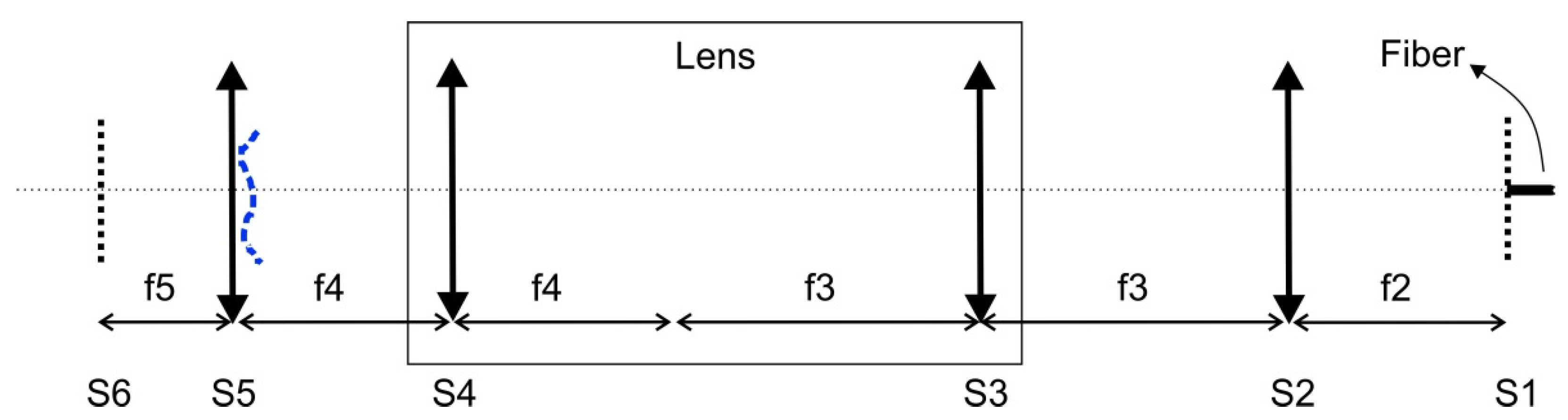
Consider the object arm of the spectral-domain OCT device (Figure 1). The radiation from the fiber exits the S1 plane and is focused in the S6 plane and is reflected and returned to the S1 plane. The fraction of power to the fiber mode was determined.
For simulation, a single-mode fiber with a mode field diameter of 10 microns was assumed at plane S1. Using the angular spectrum method [18], fields in parallel planes were calculated. Modeling was performed for monochromatic radiation. Let us denote the wavelength as , the spatial sampling rate , the distance between the planes , and the transverse size of the plane . Then, under the condition , the equation to calculate the field can be expressed as follows:
where is the impulse response function, ) are the transverse coordinates, is the wave number, is an imaginary unit, and and are forward and inverse Fourier transforms, respectively. In the case when , instead of Equation (1), the Fresnel transfer function is used:
where .
The lens, mirror, zone plate, or aberration action were simulated by multiplying the field by the corresponding two-dimensional function (see Section 2.2). In S2, the plane field was multiplied by the function of deformable mirrors of different types or by the DLP matrix. In the case of mirrors, the field in the S2 plane was additionally multiplied by the function of a collimating lens with a focal length of f2.
The system of lenses in the S3/S4 planes transferred the field from the S2 plane to the S5 plane with the necessary magnification. In the S5 plane, the field was multiplied by aberration (blue broken line in Figure 1) and lens functions. The aberrated image of the fiber was formed at plane S6. Then, the optical system was mirrored relative to plane S6, and the field was propagated from S6 back to S1. To find the energy returned to the fiber, the scalar product of the mode and the field was calculated as follows:
where is the field at the exit from the fiber (mode), is the complex field in the fiber plane, * denotes the complex conjugation, and is the fraction of energy returned to the fiber.
2.2. DLP Matrix and Amplitude Fresnel Zone Plate
An amplitude zone plate is an amplitude mask that divides the field into zones so that transmittance radiation is focused due to diffraction. Optical aberrations can be corrected with some modifications in the mask, in addition to focusing.
As is known, an ideal lens introduces a parabolic factor into the phase front:
where is the wave number, is the focal length of the lens, and are coordinates in the plane of the lens. Supposing that additional distortions are introduced into the wavefront (for example, by the human eye system), then:
where ) is the wave aberration function and is the total phase change. Then, using the function , the amplitude zone plate as a binary mask can be implemented according to this formula:
where .
The DLP matrix consists of micromirrors that can assume two positions: rotated through the angle and relative to the normal. Accordingly, rays incident on the matrix will be divided into 2 directions. If the optical system is placed in one of the directions, then the reflected light from the DLP can be considered as having passed through the binary amplitude mask. The principle of operation of DLP is illustrated in Section 3.2.
Consider the limitations associated with the pixel structure of DLP. We can easily find the equation for the distance between two zones for a lens with a focal length :. The zone size decreases as the radius (beam/aperture size) increases. For a DLP matrix with a certain element size, the maximum radius of the amplitude mask can be found. For radius , the Fresnel zone size will be less than the DLP element size. The DLP matrix DLP4500NIR from Texas Instruments with a square element size of 7.6 μm (with 912 × 1140 elements) was used in the study. The choice of this matrix was due to its design for infrared radiation, and it is a commercially available device. Using the equation above, the maximum beam diameter was approximately 17 mm, while the DLP size was about 7 × 8.7 mm. In addition, there are two effects: (1) Fresnel zones have circle geometry, while DLP elements are square. This leads to errors for the radii, including those less than ; (2) in real matrices, the size of the micromirror is about 10% less than the pixel size (there is a gap between the elements). To simulate the first effect, the field in the DLP matrix plane was sampled with a sample interval of equal to the DLP element size. The second effect was not taken into account at this stage. We assume that this will lead to a decrease in radiation intensity by about 20% due to the area of element reduction.
2.3. Focusing the Beam Using the Fresnel Plate
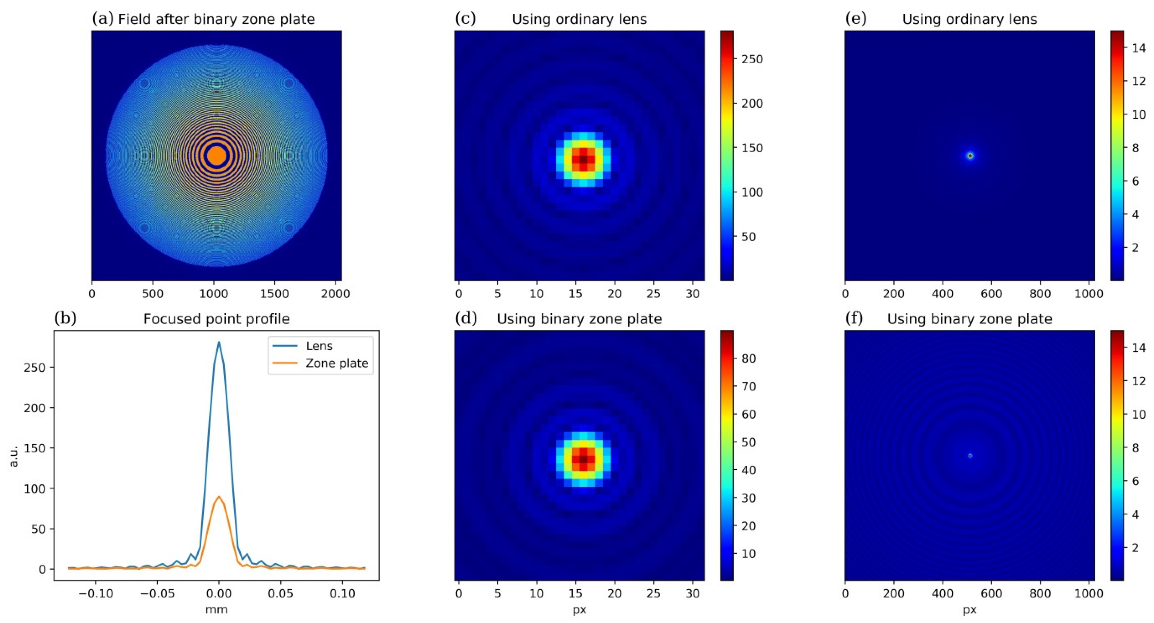
This section presents the results of modeling the focus of a Gaussian beam using a DLP matrix DLP4500NIR from Texas Instruments (the size of a square element was 7.6 μm with 912 × 1140 elements). A Gaussian beam was simulated, which was apertured by a circular diaphragm at a field level of and focused by a lens or zone plate with a focal length of 100 mm. The results are shown in Figure 2. The radiation wavelength was 850 nm.
As can be seen in Figure 2b, the beam focused by the zone plate has the same width as that focused by a conventional lens but has a field amplitude approximately 3 times smaller due to the properties of the amplitude zone plate [23]. As the power depends on the field amplitude quadratically, about 90% of the energy of the field incident on the plate is lost due to reflection and diffraction. In Figure 2f, we can see a wide “halo” around the point source image focused by the zone plate, which carries a significant amount of energy.
2.4. Modeling of Deformable Mirrors
Deformable mirrors differ in the number of actuators and the principle of their operation. In general, the greater the number of actuators, the more complex (spatially high frequency) the aberrations that can be modeled. Aberrations of the human eye are usually described by the number of Zernike polynomials from the 4th to the 8th radial degree [3,5], i.e., they contain from 12 to 45 orthogonal functions in the Zernike decomposition. The deformable mirror must have at least the same or a greater number of actuators. The typical number of actuators in deformable mirrors ranges from several tens to several thousand. As a rule, their price increases greatly with the increase in the number of actuators.
Using DLP, a binary amplitude mask can be simulated. The Fresnel zone size is a limitation in this case, which depends on the simulated lens focal length (see Section 2.2.) and, in fact, does not depend on the magnitude of the optical aberrations. Below, it will be experimentally shown that with the help of a DLP, not only can aberrations be compensated/introduced, but a holographic plate can also be realized.
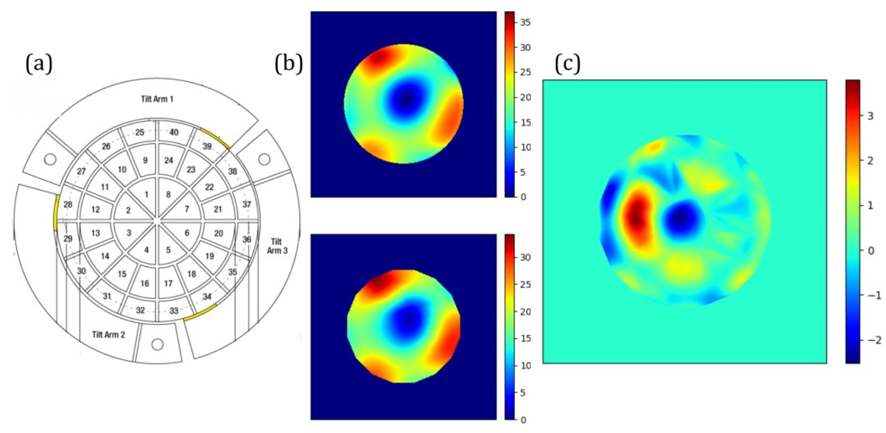
For mirror modeling, we considered that the aberration function was known in the center of each actuator. We constructed a new function which was equal in the centers of the actuators. In the case of the piezoelectric mirror (DMP40/M-F01), activation of one actuator deformed the entire mirror, so a cubic spline was applied between the actuators’ centers. In the case of the microelectromechanical system (MEMS) mirror (DM140A), according to the manufacturer’s documentation, the mirror’s pieces are individually locally sloped, so a linear spline was used. Links to the mirrors’ manufacturer’s documentation are provided in the supplementary section.
In Figure 3b,c are shown the functions , and the difference between them. The root-mean-square deviation (RMSD) of the original function was about 7 radians with an amplitude of approximately 35 radians. The RMSD of the difference between and was approximately 1 rad. For the demonstration, a large-scale aberration was taken from [24], corresponding to a numerical aperture of 0.2.
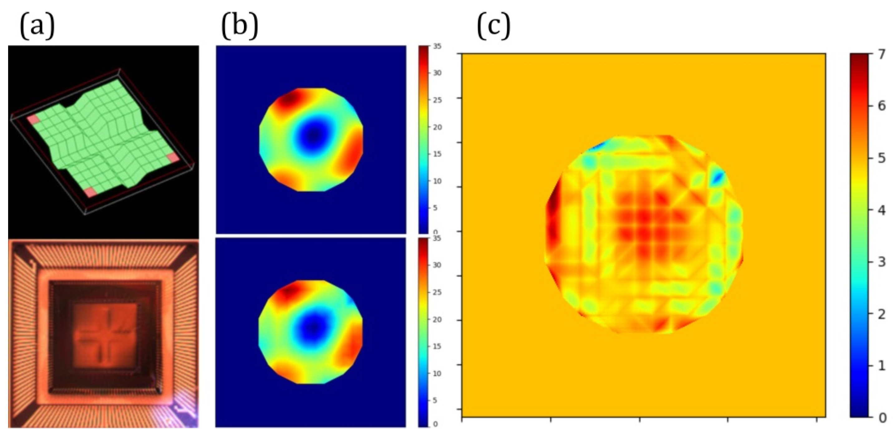
The MEMS mirror DM140A was an array of 12 × 12 elements. The tilt of each element could be set individually. As in the previous case, the phase value was found at the center of each element, after which the function was constructed using a linear spline. The results are shown in Figure 4b. The standard deviation of the function’s difference (Figure 4c) was 0.6 rad.
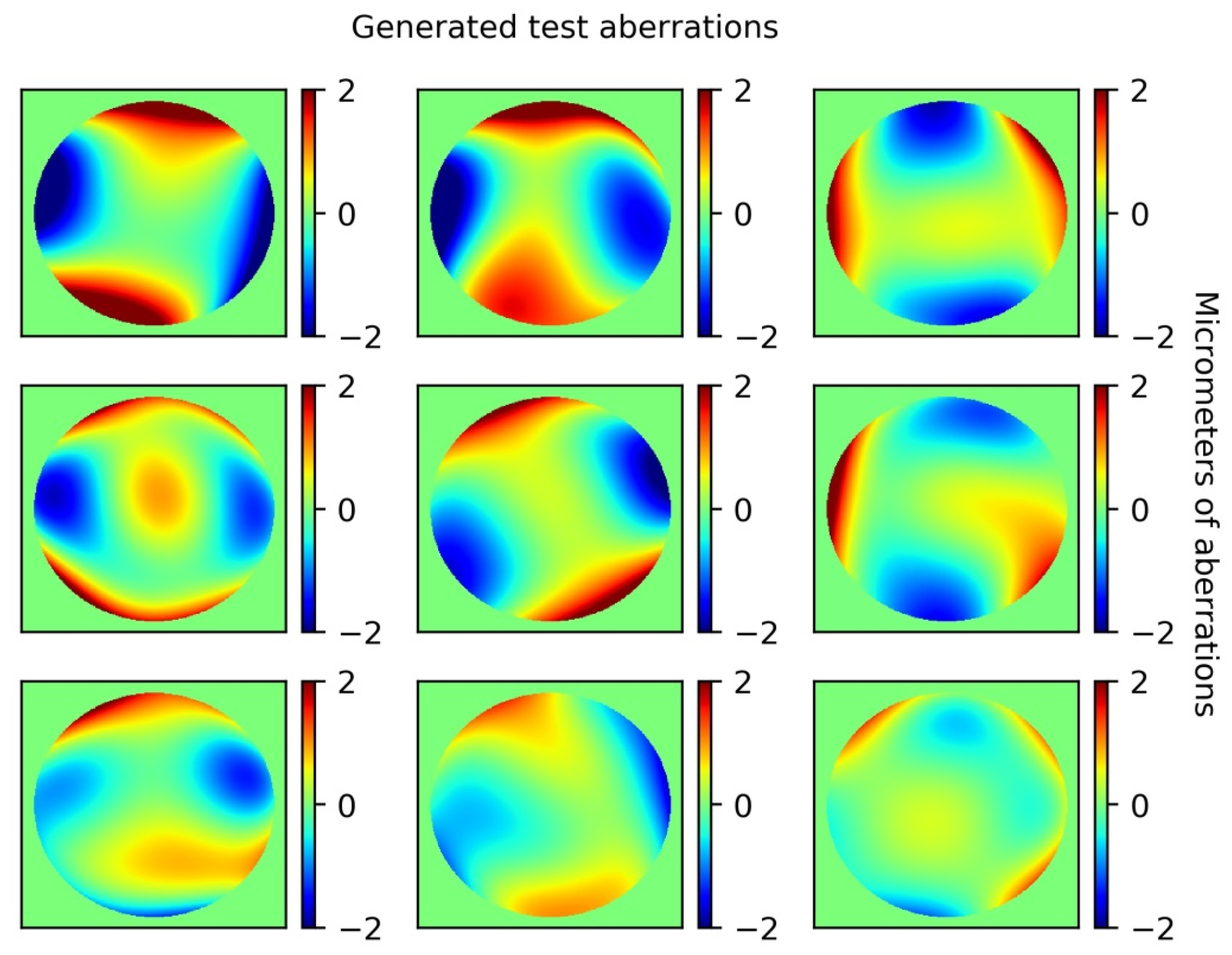
For modeling, the set of ten aberration functions was generated for a pupil with a diameter of 5.7 mm (numerical aperture ≈ 0.17). For the generation, the Zernike coefficients were used, the mean and variance of which were obtained from the study [25]. They are presented in Appendix A. Ten different aberration functions were generated.
3. Results
3.1. Simulation Results
Since the Zernike coefficients had a significant variance, the resulting aberrations were different. For each of these aberrations, the fraction of energy returned to the fiber was calculated (according to Equation (3)). The result was a set of 10 values for each of the different aberration compensators (mirrors or zone plate) and without them. For this set, the means and variances were calculated, which are presented in Table 1.
The table shows that the mirrors yielded results of comparable quality. With a piezo mirror, slightly better quality was obtained, as well as a greater variance. A MEMS mirror costs much more, but its quality, in this case, was comparable to the cheaper mirror. We found that this was due to: (a) the relatively low spatial frequency of aberrations; at a higher frequency, 40 piezoelectric actuators might not be sufficient to form a wavefront of proper quality; and (b) due to the square geometry of the MEMS mirror, only about 100 of the 144 actuators participated in the wavefront fitting.
The DLP matrix functioned noticeably worse than the mirrors. At the same time, the value of the returned energy had a relatively low dispersion. Thus, the efficiency of the DLP matrix weakly depended on the type and scale of the aberrations. With this sample and at this pupil size, such a system allowed an approximately five-fold increase in the effectiveness of reception. In addition, image defocusing was not taken into account during modeling (usually in OCT tomographs, it is compensated physically). However, in [25], an 80% RMS wavefront error was indicated. Residual defocusing can also be easily compensated with the help of the DLP matrix system, which increases its effectiveness.
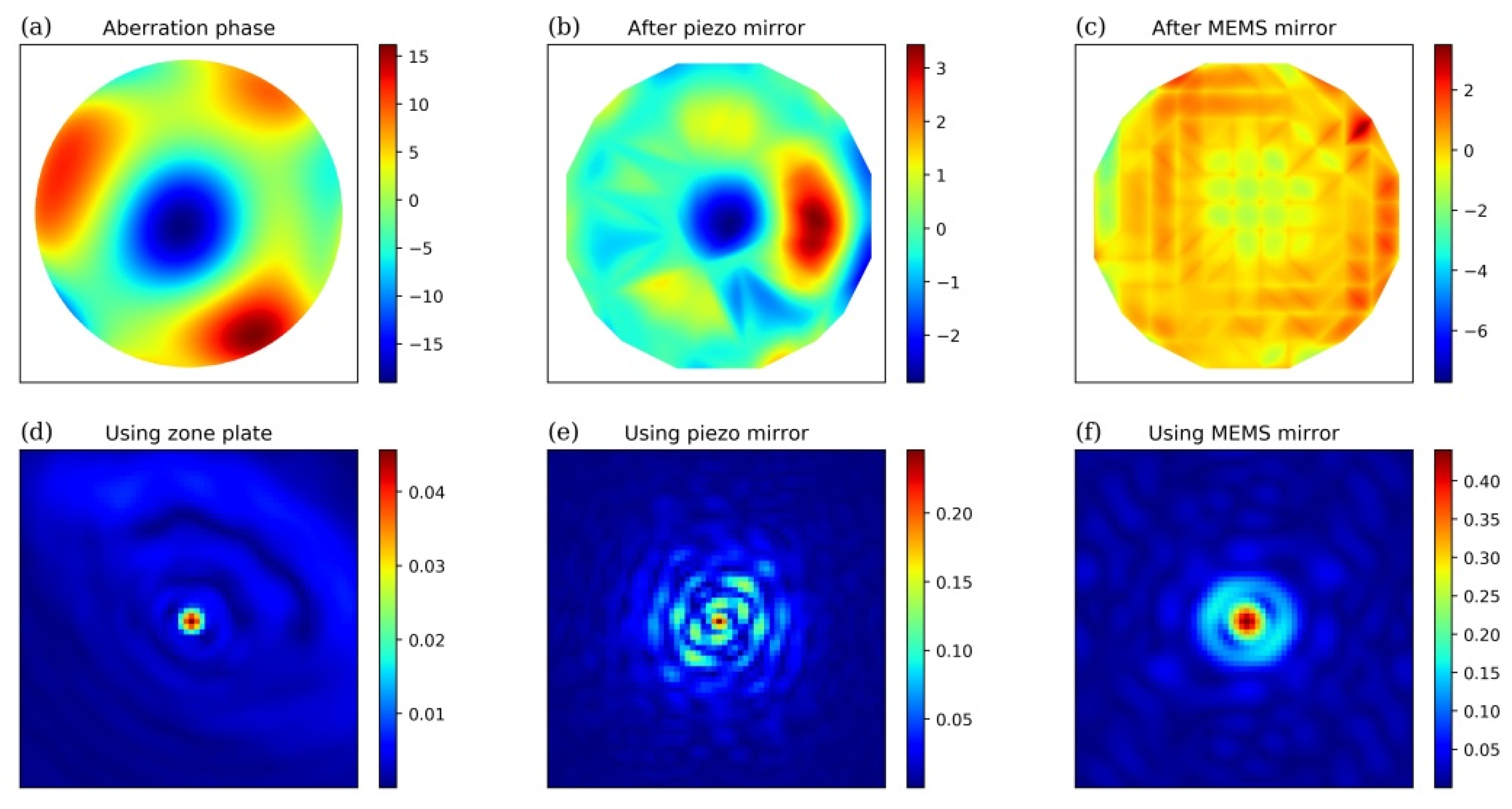
Figure 5 shows a simulation of the effect of wavefront correctors with an eye pupil of 7 mm and the aberration obtained from a previous study [24] (the generated amplitude zone plate to simulate image 5d is presented in Figure A3). Based on this, we can conclude that the zone plate produces an image of the point with the smallest width, but a large amount of energy is lost due to reflection and diffraction. In this case, the MEMS mirror showed a noticeably better result than the piezoelectric mirror, which was due to the presence of high-frequency components in the spatial aberration spectrum (the presence of high Zernike polynomials). The amount of energy returned to the fiber for the zone plate, piezo, and MEMS mirrors is 0.076, 0.122, and 0.46, respectively.
3.2. Experimental Results
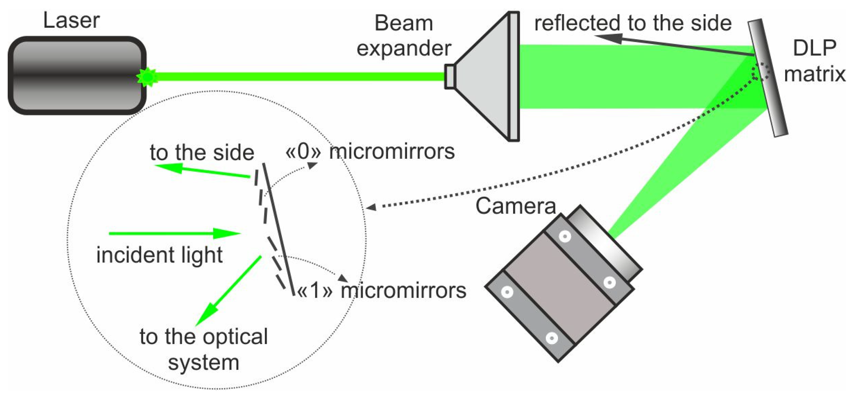
To demonstrate the possibility of using a DLP matrix for aberration compensation, an experimental apparatus was assembled, shown in Figure 6. For this apparatus, a green laser beam (Melles Griot LGR-025-450) with a wavelength of 544 nm was expanded on a beam expander and fell on the DLP matrix. A DLP with a driving unit was the commercially available projector (Philips PicoPix Micro). The diffraction pattern was sent to the HDMI input. The DLP matrix was taken out of the projector box but was driven by projector electronics. There were no markings on the case of the DLP, but based on its geometry, it was assumed to be a Texas Instruments DLP230GP with 960 × 540 square pixels of 5.4 × 5.4 µm. The images obtained using DLP were registered with a Thorlabs DCC1545M camera with 1280 × 1024 square pixels with a size of 5.2 µm.
The DLP matrix is a periodic structure with a specific gap between the micromirrors. Thus, it can be considered as a reflective diffraction grating with a period equal to the pixel size. Therefore, the DLP matrix was tilted at an angle so that the diffraction angle was equal to the reflection angle.
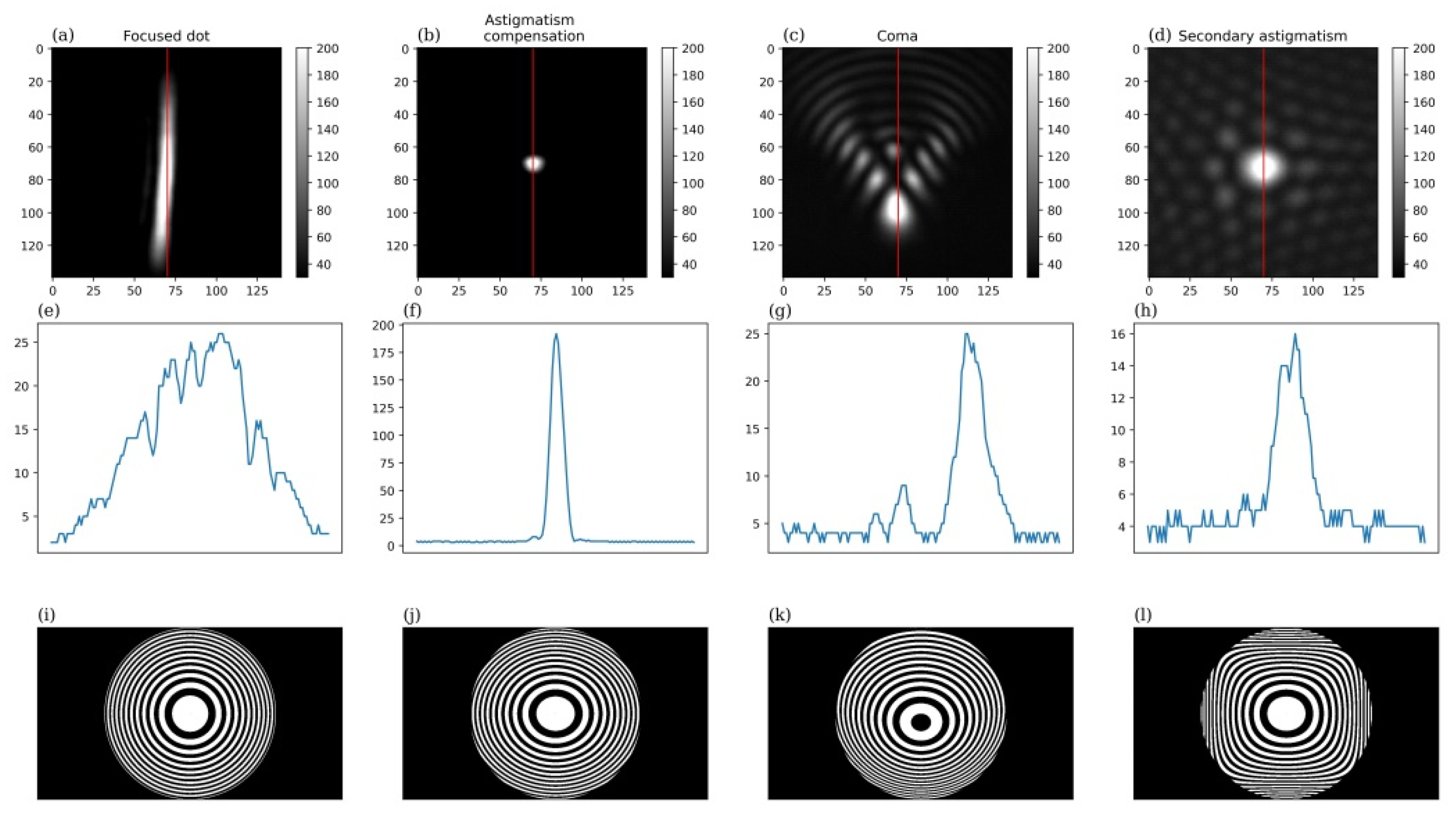
Figure 7 presents images of the AZP focused laser beam. There was significant astigmatism in this system, which can be seen in the first column of Figure 7. This was compensated by modifying the AZP by inserting an astigmatism term (the coefficient before the term was hand-fitted). The result is shown in the second column in Figure 7. In the third and fourth columns of Figure 7, coma and secondary astigmatism were additionally introduced, respectively, where 3 and 5 are coefficients before the polynomials. We see that the resulting images qualitatively correspond to the images of a point spread function with the coma/astigmatism aberrations.
The images in Figure 7a–d were obtained at different camera exposures. The brightness of the images was normalized between 0 and 255 for better visibility. The second row presents the intensities along the red lines in the images in the first row. However, in this case, exposure time was fixed (0.2 ms). The third row presents diffraction masks, corresponding to the images above.
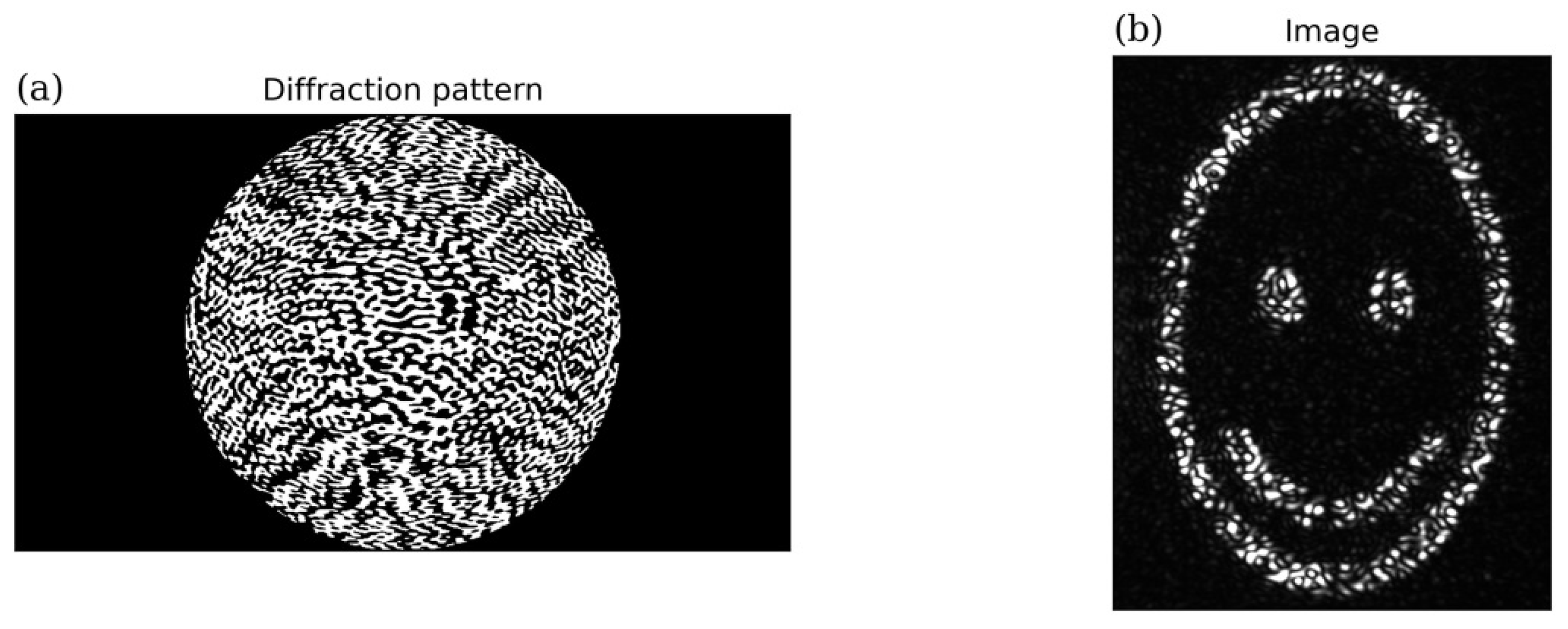
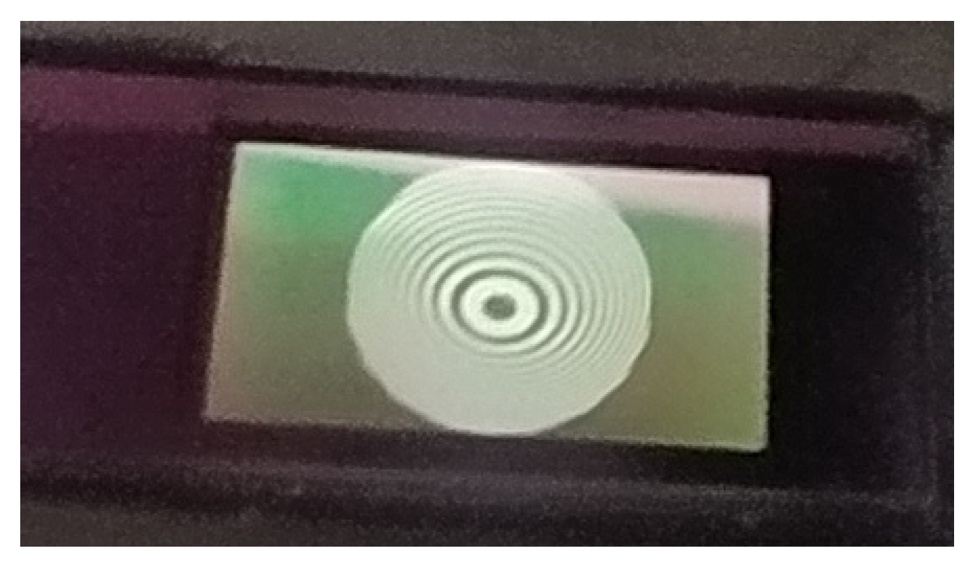
To show the possibility of phase control using DLP, a special pattern was synthesized that would produce an image in the focus area (which, in fact, is the implementation of a holographic plate). For this, an image (smile) was taken, and the argument of its Fourier transform was found. Then, the lens phase was added to the resulting function (Equation (4)). Based on the resulting function, using Equation (6), the diffraction pattern was synthesized, as shown in Figure 8a. The obtained image is shown in Figure 8b.
These experiments demonstrate that it is possible to introduce/correct very significant phase distortions with the assistance of DLP. At the same time, the experimental portion was performed on a device costing a total of approximately USD 250.
4. Discussion
This study provides a theoretical justification for the possibility of using a DLP matrix as an element of an adaptive optics system with spectral-domain OCT devices. Using a numerical simulation, it was possible to increase the amount of received radiation by approximately 5 times (for aberrations of a 5.7 mm eye pupil diameter) compared with the absence of aberration compensation. Numerical modeling showed that aberrations with large amplitudes can be compensated using an adaptive zone plate. With sufficiently large aberrations, the efficiency of the DLP matrix becomes comparable to the efficiency of traditional mirrors. Thus, in the image in Figure 5, DLP and the piezo mirror yielded efficiencies of 0.076 and 0.122, respectively. In addition, the zone plate led to a large loss of light; therefore, it was possible to increase the power of the probe beam without the risk of exceeding the permissible norms for the retina. Thus, the efficiency values of received radiation, when using a zone plate, can be doubled.
The larger the aberrations are, the greater the benefit of using a zone plate and the smaller the gap compared to traditional deformable mirrors. Taking into account the rather large variance in the aberrations (0.016 ± 0.012 in Table 1), in some cases, it is possible without compensation, and in some cases, there is almost no signal and compensation is necessary. Using DLP always returns the signal to a certain preset level, since the main power losses are due to diffraction and not to aberrations. Thus, the system efficiency does not depend on the presence of aberrations and becomes predictable.
It is also worth mentioning that the DLP matrix has a high speed of operation, which is important for adaptive optics systems.
From the presented study, it can be concluded that the use of an adaptive zone plate can make it possible to implement a relatively inexpensive system with adaptive optics, which will be especially useful for cases with large aberrations.
Author Contributions
Conceptualization, A.M. and G.G.; methodology, V.M., A.M. and P.S.; software, V.M.; validation, G.G., V.M. and P.S.; writing—original draft preparation, V.M.; writing—review and editing, G.G., A.M. and P.S. All authors have read and agreed to the published version of the manuscript.
Funding
The study was supported by the WorldClass Research Centre “Photonics Centre” under the financial support of the Ministry of Science and High Education of the Russian Federation (Agreement No. 075-15-2020-906).
Data Availability Statement
Data from the experimental setup can be found at the link https://github.com/vasilymat/article7.
Conflicts of Interest
The authors declare no conflict of interest. The funders had no role in the design of the study; in the collection, analyses, or interpretation of data; in the writing of the manuscript, or in the decision to publish the results.
Appendix A
In Figure A1, the blue lines represent the means and variances of the Zernike coefficients, corresponding to Figure 3 of [25].
Figure A1.
Generating sets of Zernike coefficients. Each of the ten sets is marked with different-colored circle markers. The blue vertical lines mark the variance value of the corresponding Zernike coefficient. The x-axis shows the numbers of the coefficients in Noll’s notation; the y-axis shows the values of the coefficients in micrometers.

Using these statistics, we generated 10 sets of Zernike coefficients. The values of the generated coefficients are presented in Figure A1 with round markers of various colors. Afterwards, using the set of coefficients, the set of aberration functions was generated (sums of Zernike polynomials with corresponding coefficients). The first nine of them are shown in Figure A2.
Figure A2.
Generated aberration functions using the Zernike coefficients sets. The first nine individual functions.
Figure A2.
Generated aberration functions using the Zernike coefficients sets. The first nine individual functions.

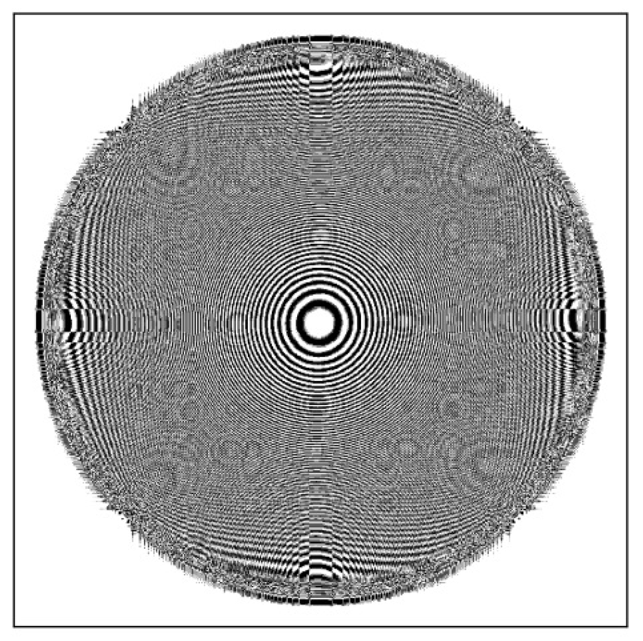
Figure A3.
AZP for aberration related to Figure 5d.
Figure A3.
AZP for aberration related to Figure 5d.

Figure A4 presents the photo of a DLP matrix with a binary mask of an aberrated lens.
Figure A4.
Photo of a binary mask, generated by the DLP matrix.

References
- Goncharov, A.S.; Iroshnikov, N.G.; Larichev, A.V. Retinal Imaging: Adaptive Optics. In Handbook of Coherent-Domain Optical Methods: Biomedical Diagnostics, Environmental Monitoring, and Materials Science; Tuchin, V.V., Ed.; Springer New York: New York, NY, USA, 2013; pp. 397–434. [Google Scholar]
- Kumar, A.; Drexler, W.; Leitgeb, R.A. Subaperture correlation based digital adaptive optics for full field optical coherence tomography. Opt. Express. OSA 2013, 21, 10850–10866. [Google Scholar] [CrossRef] [PubMed]
- Shemonski, N.D.; South, F.A.; Liu, Y.; Adie, S.G.; Carney, P.S.; Boppart, S.A. Computational high-resolution optical imaging of the living human retina. Nat. Photonics 2015, 9, 440–443. [Google Scholar] [CrossRef] [PubMed] [Green Version]
- Moiseev, A.A.; Gelikonov, G.V.; Shilyagin, P.A.; Gelikonov, V.M. Using phase gradient autofocus (PGA) algorithm for restoration OCT images with diffraction limited resolution. In Optical Coherence Tomography and Coherence Domain Optical Methods in Biomedicine; Proc. SPIE 7999, Saratov Fall Meeting 2010; SPIE: Bellingham, WA, USA, 2011. [Google Scholar]
- Hillmann, D.; Spahr, H.; Hain, C.; Sudkamp, H.; Franke, G.; Pfäffle, C.; Winter, C.; Hüttmann, G. Aberration-free volumetric high-speed imaging of in vivo retina. Sci. Rep. 2016, 6, 35209. [Google Scholar] [CrossRef] [PubMed] [Green Version]
- Hillmann, D.; Pfäffle, C.; Spahr, H.; Burhan, S.; Kutzner, L.; Hilge, F.; Hüttmann, G. Computational adaptive optics for optical coherence tomography using multiple randomized subaperture correlations. Opt. Lett. OSA 2019, 44, 3905–3908. [Google Scholar] [CrossRef] [PubMed]
- Matkivsky, V.A.; Moiseev, A.A.; Gelikonov, G.V.; Shabanov, D.V. Correction of aberrations in digital holography using the phase gradient autofocus technique. Laser Phys. Lett. 2016, 13, 35601. [Google Scholar] [CrossRef]
- Ginner, L.; Kumar, A.; Fechtig, D.; Wurster, L.M.; Salas, M.; Pircher, M.; Leitgeb, R.A. Noniterative digital aberration correction for cellular resolution retinal optical coherence tomography in vivo. Optica 2017, 4, 924–931. [Google Scholar] [CrossRef]
- South, F.A.; Kurokawa, K.; Liu, Z.; Liu, Y.Z.; Miller, D.T.; Boppart, S.A. Combined hardware and computational optical wavefront correction. Biomed. Opt. Express. OSA 2018, 9, 2562–2574. [Google Scholar] [CrossRef] [PubMed]
- Matveyev, A.L.; Matveev, L.A.; Moiseev, A.A.; Sovetsky, A.A.; Gelikonov, G.V.; Zaitsev, V.Y. Simulating scan formation in multimodal optical coherence tomography: Angular-spectrum formulation based on ballistic scattering of arbitrary-form beams. Biomed. Opt. Express. OSA 2021, 12, 7599–7615. [Google Scholar] [CrossRef] [PubMed]
- Pircher, M.; Zawadzki, R.J. Review of adaptive optics OCT (AO-OCT): Principles and applications for retinal imaging [Invited]. Biomed. Opt. Express. OSA 2017, 8, 2536–2562. [Google Scholar] [CrossRef] [PubMed]
- Bernet, S.; Harm, W.; Ritsch-Marte, M. Demonstration of focus-tunable diffractive Moiré-lenses. Opt. Express. OSA 2013, 21, 6955–6966. [Google Scholar] [CrossRef] [PubMed]
- Chen, L.; Ghilardi, M.; Busfield, J.J.C.; Carpi, F. Electrically Tunable Lenses: A Review. Front. Robot. AI Front. Media SA 2021. [Google Scholar] [CrossRef] [PubMed]
- Romero, L.A.; Millán, M.S.; Jaroszewicz, Z.; Kolodziejczyk, A. Programmable Diffractive Optical Elements for Extending the Depth of Focus in Ophthalmic Optics. In Proceedings of the 10th International Symposium on Medical Information Processing and Analysis. International Society for Optics and Photonics, Cartagena de Indias, Colombia, 14–16 October 2014; Volume 9287, p. 92871E. [Google Scholar]
- Li, G.; Mathine, D.L.; Valley, P.; Ayräs, P.; Haddock, J.N.; Giridhar, M.S.; Williby, G.; Schwiegerling, J.; Meredith, G.R.; Kippelen, B.; et al. Switchable electro-optic diffractive lens with high efficiency for ophthalmic applications. Proc. Natl. Acad. Sci. USA 2006, 103, 6100–6104. [Google Scholar] [CrossRef] [PubMed] [Green Version]
- Wang, P.; Mohammad, N.; Menon, R. Chromatic-aberration-corrected diffractive lenses for ultra-broadband focusing. Sci. Rep. 2016, 6, 1–7. [Google Scholar] [CrossRef] [PubMed] [Green Version]
- Ghilardi, M.; Boys, H.; Török, P.; Busfield, J.J.C.; Carpi, F. Smart Lenses with Electrically Tuneable Astigmatism. Sci. Rep. 2019, 9, 16127. [Google Scholar] [CrossRef] [PubMed] [Green Version]
- Kipp, L.; Skibowski, M.; Johnson, R.L.; Berndt, R.; Adelung, R.; Harm, S.; Seemann, R. Sharper images by focusing soft X-rays with photon sieves. Nature 2001, 414, 184–188. [Google Scholar] [CrossRef] [PubMed]
- Oktem, F.S.; Kamalabadi, F.; Davila, J.M. Analytical Fresnel imaging models for photon sieves. Opt. Express 2018, 26, 32259–32279. [Google Scholar] [CrossRef] [PubMed]
- Oktem, F.S.; Kar, O.F.; Bezek, C.D.; Kamalabadi, F. High-resolution multi-spectral imaging with diffractive lenses and learned reconstruction. IEEE Trans. Comput. Imaging 2021. [Google Scholar] [CrossRef]
- Hallada, F.D.; Franz, A.L.; Hawks, M.R. Fresnel zone plate light field spectral imaging. Opt. Eng. 2017, 56, 1–11. [Google Scholar] [CrossRef]
- Yang, Y.; Zhang, Y.; Zhang, J.; Li, Y.; Liu, D.; Zhu, J. Shack-Hartmann wavefront sensing with super-resolution photon-sieve array. In 4th Optics Young Scientist Summit (OYSS 2020); International Society for Optics and Photonics; SPIE: Bellingham, WA, USA, 2021; Volume 11781, p. 117810T. [Google Scholar]
- Breckinridge, J.B.; Voelz, D.G. Computational fourier optics: A MATLAB tutorial. In Society of Photo-Optical Instrumentation Engineers; SPIE Press: Bellingham, WA, USA, 2011. [Google Scholar]
- Matkivsky, V.; Moiseev, A.; Shilyagin, P.; Rodionov, A.; Spahr, H.; Pfäffle, C.; Hüttmann, G.; Hillmann, D.; Gelikonov, G. Determination and correction of aberrations in full field optical coherence tomography using phase gradient autofocus by maximizing the likelihood function. J. Biophotonics. 2020, 13, e202000112. [Google Scholar] [CrossRef] [PubMed]
- Porter, J.; Guirao, A.; Cox, I.G.; Williams, D.R. Monochromatic aberrations of the human eye in a large population. J. Opt. Soc. Am. A. Opt. Image Sci. Vis. 2001, 18, 1793–1803. [Google Scholar] [CrossRef] [PubMed] [Green Version]
Figure 1.
Optical scheme for the deformable mirror/Fresnel plate modeling. Radiation is emitted from the fiber in the center of the S1 plane. In the case of deformable mirror modeling, a combined phase mask (deformable mirror plus the lens with f2 focal length) is placed in the S2 plane. In the case of DLP modeling, a corresponding binary mask is placed in the S2 plane. The combination of lenses in the S3 and S4 planes transfers the field from the S2 to the S5 plane. A lens in the S5 plane focuses radiation in the S6 plane. Aberrations are inserted into the S5 plane (marked with a blue dotted line).

Figure 2.
Beam focusing. (a) The modulus of the field passed through the Fresnel zone plate; (b) point source in-focus profiles (x-axis is measured in millimeters). Orange line—using the zone plate, blue—using an ordinary lens of the same focal length; (c,d) images of a point source using the lens and the zone plate, respectively; (e,f) images matching images (c,d) but with large field of view (1024 px. instead of 32). The values of the color scales have been changed for wide “halo” highlighting in image (f) (the values of the modulus of the field themselves remained unchanged). The x-axes are measured in pixels, and the size of the x-axis is equal to the y-axis for all images except (b). Color bars are displayed as field strength in arbitrary units (a.u.). Pixel size is 3.8 µm.

Figure 3.
Piezoelectric mirror modeling. (a) Mirror actuators (according to the documentation from the manufacturer’s website); (b) initial phase and phase of the mirror obtained by simulation; (c) difference between the phases from Figure (b). Color bars are in radians.
Figure 3.
Piezoelectric mirror modeling. (a) Mirror actuators (according to the documentation from the manufacturer’s website); (b) initial phase and phase of the mirror obtained by simulation; (c) difference between the phases from Figure (b). Color bars are in radians.

Figure 4.
MEMS mirror modeling. (a) Mirror segments (according to the documentation from the manufacturer’s website); (b) initial phase and phase of the mirror obtained by simulation; (c) the difference between the phases from Figure (b). Color bars are in radians.
Figure 4.
MEMS mirror modeling. (a) Mirror segments (according to the documentation from the manufacturer’s website); (b) initial phase and phase of the mirror obtained by simulation; (c) the difference between the phases from Figure (b). Color bars are in radians.

Figure 5.
Residual aberrations and calculated field amplitude at the fiber end. (a) Initial aberration in radians; (b,c) residual aberrations for piezo and MEMS mirrors, respectively; (d–f) field amplitude at the fiber end when using zone plate, piezo, and MEMS correctors, respectively (in arbitrary units).

Figure 6.
Experimental apparatus. The dashed circle illustrates the principle of DLP matrix operation. Micromirror “0” reflects light to the side, and micromirror “1” reflects light into the camera/optical system.
Figure 6.
Experimental apparatus. The dashed circle illustrates the principle of DLP matrix operation. Micromirror “0” reflects light to the side, and micromirror “1” reflects light into the camera/optical system.

Figure 7.
Focusing a laser beam with the AZP. The first row (a–d) shows images of a beam, focused with the AZP patterns from the third row (i–l). In the first column, AZP has a focal length of 150 mm. In the second column, astigmatism was compensated. In the third and fourth columns, coma and secondary astigmatism were additionally introduced. In the second row (e–h) are graphs of the intensities along the red lines in the first row (at a fixed camera exposure).

Figure 8.
DLP as a holographic plate. (a) Diffraction pattern; (b) image in focal plane.


Table 1.
Comparison of return-to-fiber efficiency for different aberration-compensation methods.
| With Compensation | Without Compensation | |
|---|---|---|
| Piezoelectric mirror | 0.80 ± 0.15 | 0.016 ± 0.012 |
| MEMS mirror | 0.77 ± 0.07 | |
| DLP matrix | 0.077 ± 0.003 |
Publisher’s Note: MDPI stays neutral with regard to jurisdictional claims in published maps and institutional affiliations. |
© 2022 by the authors. Licensee MDPI, Basel, Switzerland. This article is an open access article distributed under the terms and conditions of the Creative Commons Attribution (CC BY) license (https://creativecommons.org/licenses/by/4.0/).
Share and Cite
MDPI and ACS Style
Matkivsky, V.; Moiseev, A.; Shilyagin, P.; Gelikonov, G. Amplitude Zone Plate in Adaptive Optics: Proposal of the Principle. Photonics 2022, 9, 163. https://doi.org/10.3390/photonics9030163
AMA Style
Matkivsky V, Moiseev A, Shilyagin P, Gelikonov G. Amplitude Zone Plate in Adaptive Optics: Proposal of the Principle. Photonics. 2022; 9(3):163. https://doi.org/10.3390/photonics9030163
Chicago/Turabian StyleMatkivsky, Vasily, Alexsandr Moiseev, Pavel Shilyagin, and Grigory Gelikonov. 2022. "Amplitude Zone Plate in Adaptive Optics: Proposal of the Principle" Photonics 9, no. 3: 163. https://doi.org/10.3390/photonics9030163
Note that from the first issue of 2016, this journal uses article numbers instead of page numbers. See further details here.