Linearity and Optimum-Sampling in Photon-Counting Digital Holographic Microscopy

Abstract

In the image plane configurations frequently used in digital holographic microscopy (DHM) systems, interference patterns are captured by a photo-sensitive array detector located at the image plane of an input object. The object information in these patterns is localized and thus extremely sensitive to phase errors caused by nonlinear hologram recordings (grating profiles are either square or saturated sinusoidal) or inadequate sampling regarding the information coverage (undersampled around the Nyquist frequency or arbitrarily oversampled). Here, we propose a solution for both hologram recording problems through implementing a photon-counting detector (PCD) mounted on a motorized XY translation stage. In such a way, inherently linear (because of a wide dynamic range of PCD) and optimum sampled (due to adjustable steps) digital holograms in the image plane configuration are recorded. Optimum sampling is estimated based on numerical analysis. The validity of the proposed approach is confirmed experimentally.

1. Introduction

Diverse optical-hybrid solutions have been developed in digital holographic microscopy (DHM) [1,2], from the simplest optical setups known as the lensless DHMs to the most frequently exploited imaging configurations. While the lensless DHM configurations are particularly attractive due to their compactness and robustness prospects [3,4], the later image plane setups are mostly preferred due to the flexibility and efficacy of (i) light collection, (ii) optical magnification, and (iii) pixel usage of local hologram data [5]. For real-world applications, quality recording of the entire hologram is a crucial operation since the object information is locally constrained rather than spread throughout the detector. When recording a sinusoidal fringe pattern, the continuous analog input is sampled to produce a discrete pattern which consequently suffers from various defects. We expect accurate phase information from the recorded digital hologram (DH). In obtaining the phase information, there are several problems, such as speckle [6,7] or shot noise [8]. Another effect, a rolling shutter aberration caused by the sequential readout nature of some detectors, has also been studied, and a method for compensating this effect in an image plane DHM has been proposed [9]. In temporal phase-shifting DHM, it was demonstrated that a partially coherent light source (LED) yields a lower phase noise than a coherent one (laser) [10]. In the field of electronic speckle pattern interferometry (ESPI), the periodic phase reconstruction errors were studied, and the noise reduction was proposed within the spatial phase-shifting technique [11]. Apart from these problems, for the correct phase calculation, special care should be focused on the deviation from linearity of the holographic grating (profiles such as saturated sinusoidal profile or square profile) and particularly on the sampling conditions.

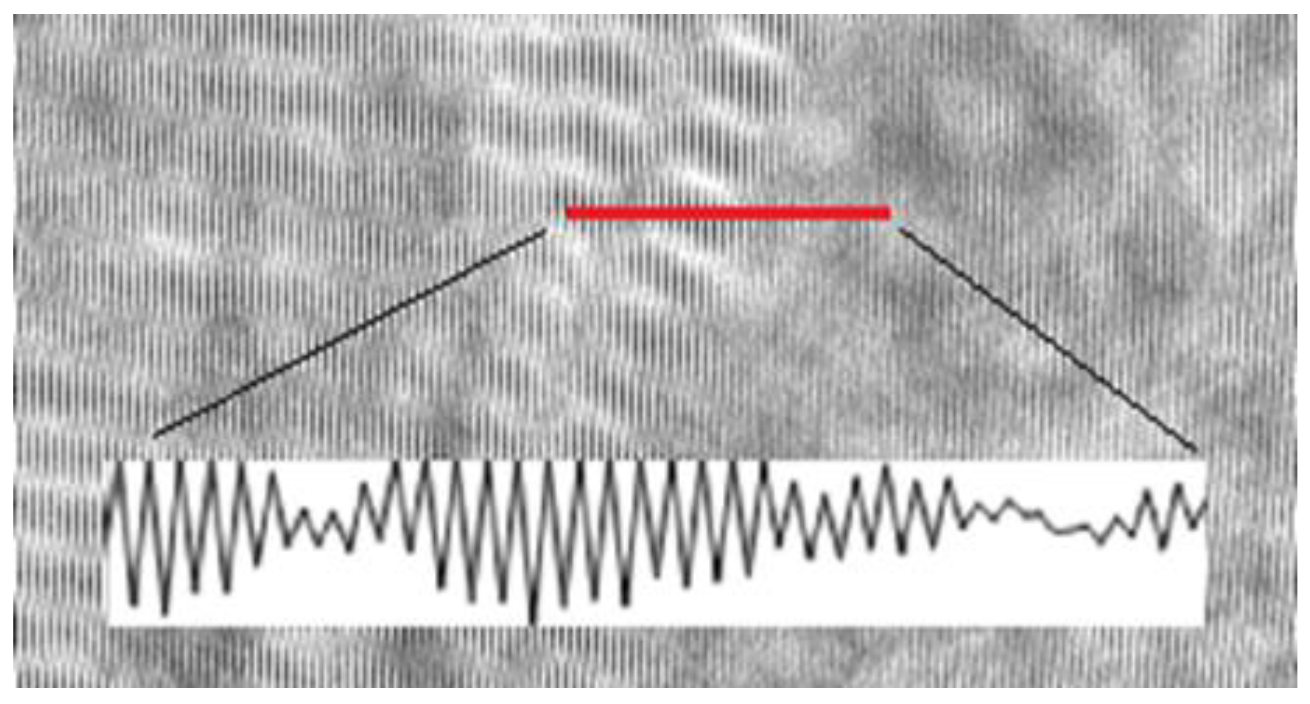
A typical sampling and nonlinearity problem that occurs in the image plane setups is illustrated in Figure 1. We show a part of an image plane hologram recorded at the Nyquist sampling rate with 8-bit gray levels. The areas with high contrast fringes and areas in which the interference pattern is lost (or having very low contrast due to the beating effect) can be easily spotted. The cross-section along the red line of Figure 1 shows the locations with the information loss that cannot be recovered for that part of the object.

Figure 1 demonstrates that in the image plane setups, where the object information is localized at the detector’s plane, the sampling necessary condition is not withal sufficient. In other architectures, such as Fresnel and Fourier setups, the Nyquist rate is usually sufficient for sampling data since the object wavefront information is non-localized (every point on the object potentially contributes to every hologram pixel), and thus the information is preserved. In addition to the loss of information, we can easily notice that the recorded grating is not of the sinusoidal profile, and it is saturated (at 255 gray level).

Nonlinear hologram gratings cause the appearance of not only the higher diffraction terms in the reconstructed field but also the phase errors [12,13,14]. Such experimental errors have been identified in phase-shifting interferometry [12] and well analyzed and compensated by an iterative algorithm in phase-shifting digital fringe projection profilometry [13]. In Ref. [14], the phase demodulation errors involved in analyzing single-frame fringe patterns were studied, and the advanced variational image decomposition technique proposed to reduce the errors such as random noise and nonlinearity, where for weaker noise, the nonlinearity was identified as the dominant source of phase errors. Therefore, nonlinearities persist in the DHM systems as a concomitant recording problem.

The sampling conditions have been well studied in the DH systems [15,16,17,18,19,20,21]. In brief, for a band-limited input optical signal with the size L and spatial frequency bandwidth W, the information density or its space-bandwidth product (SBP) can be defined as SBP = LW, where only one dimension is considered for simplicity. The cost-effective optical system ought to have its SBP capacity slightly greater or equal to the SBP of the signal. In the DH systems, there are differences between the SBPs of the input signal, the recording sensor, and the reconstructed signal. These differences are due to the wavefront propagation configuration (Fresnel, Fourier, or image plane), the object/reference beams geometry (on-axis or off-axis), and the resolution properties of the array detector, as discussed, for example, in Ref. [15]. The least demanding configuration concerning the recording sensor is the Fourier configuration, while the introduction of lenses should be generally avoided unless the object is too small, as is the case of the DHM. Although the phase information will not be reconstructed properly if the Nyquist condition is not satisfied, a variety of possibilities as well as techniques to overcome this limitation exist. The full recovery of the undersampled Fresnel diffraction patterns can be achieved for the finite-sized input objects by windowing the backpropagating field [16]. Also, in the off-axis quasi-Fourier setup, the effects of increasing the angle between the reference and object beams beyond the Nyquist limit on the hologram reconstruction were analyzed both theoretically and experimentally [17]. For a given input object bandwidth, it was shown that the reconstructed image of the object is repeatedly folding and inverting (passing through non-overlapping intervals) until the image faded out. It was also demonstrated that these non-overlapping intervals could be significantly extended by applying the subtraction digital holography method [17,18]. The influence of the pixel dimension for hologram recordings beyond the Shannon limits was also investigated [19]. The space bandwidth available for recording an object wave in an off-axis configuration was extended by intentionally setting the aliasing to the recorded hologram [20]. In yet another study, it was shown that the aliasing-free DHM with resolution equal to the diffraction limit of the lensless system could be achieved for partly coherent light [21].

In this paper, we present a new approach to holographic recordings that are (i) always linear (sinusoidal) and (ii) optimally sampled (minimum redundancy). The proposed approach employs a photon-counting detector (PCD) for recording digital holograms in a DHM system with an image plane configuration. The PCD was already used in the DH systems [22,23,24]. First, the recording of a digital hologram was demonstrated for the signal light intensity above the dark count noise of the detector [22]. Later, the recording of holograms was extended to the signal light levels that were significantly below dark count noise [23], as well as to the recording of time-averaged holograms [24]. Here, we take advantage of the PCD over a standard array detector such as a charge-coupled device (CCD) in terms of pixel size flexibility and inherent recording linearity. These properties are especially beneficial in physically constrained sample volumes with fixed fringe spacing at the sensor, as presented in a compact DHM system [25].

The conditions for optimum sampling are numerically evaluated in Section 2.1, where we first explain the role of the detector’s position relative to the input sinusoidal light distribution, and then find a parameter for optimum sampling. The experimental setup is described in Section 2.2. The results is presented in Section 3, while the concluding discussion is drawn in Section 4.

2. Methods

2.1. Optimum Sampling Conditions

To preserve information, the interference pattern is required to be sampled at the Nyquist limit, i.e., the maximum spatial frequency of the pattern is restricted by $f_{max}\le f_N$, where $f_N$ is the Nyquist frequency. $f_N$ is defined by the pixel size $\Delta x$ of the detector,$f_N=1/\left(2\Delta x\right)$. The limitation imposed by the pixel size $\Delta x$ can be managed by adjusting the distance between the detector and object, by the angle between the reference and object beams, and by the apertures in the system. Since the Fourier spectrum of the sinusoidal fringe pattern contains a Dirac impulse, the sampling efficacy (fidelity) depends not only on the pixel size but also on the relative position of the pixels in relation to the phase of the sinusoidal pattern.

A sinusoidal fringe pattern can be generally described by a continuous intensity function:

$$I\left(x\right)=a\left(x\right)+b\left(x\right)sin\left[\phi \left(x\right)\right]$$

(1)

where $a\left(x\right)$ and $b\left(x\right)$ are the background and modulation intensities, respectively, and $\phi \left(x\right)$ is the desired phase. We use the one-dimensional notation of generally two-dimensional spatial coordinates for simplicity. One of the most important measurables is the contrast of fringes or the fringe visibility,

$$V\left(x\right)=\frac{b\left(x\right)}{a\left(x\right)}=\frac{\left[I_M\left(x\right)-I_m\left(x\right)\right]}{\left[I_M\left(x\right)+I_m\left(x\right)\right]},$$

(2)

where $I_M\left(x\right)$ and $I_m\left(x\right)$ are the maximum and minimum intensities, respectively. $V\left(x\right)$ varies across the fringe pattern but has nearly constant value locally (as demonstrated in Figure 1).

For numerical simulations, we take the simplified discrete form of Equation (1), representing an input signal to the detector

$$I_S\left(j\delta x\right)=1+\sin \left(2\pi f_{0}j\delta x\right)$$

(3)

where the detector plane is sampled with sampling interval $\delta x$, j denotes the number of calculation points. In Equation (3), $f_0$ is the spatial carrier frequency, $f_0=1/X$, where X is the period of fringes in the spatial domain. The calculations are further simplified by taking $X=1$. Numerical simulations are performed assuming that the parameters of input sinusoidal distribution are fixed while the parameters of the pixelated detector are variable. Furthermore, for all calculations, we take many points per detector’s pixel, ${J_{\Delta x}}^{″}1$, where $J_{\Delta x}$ is the total number of points inside one pixel $\Delta x$.

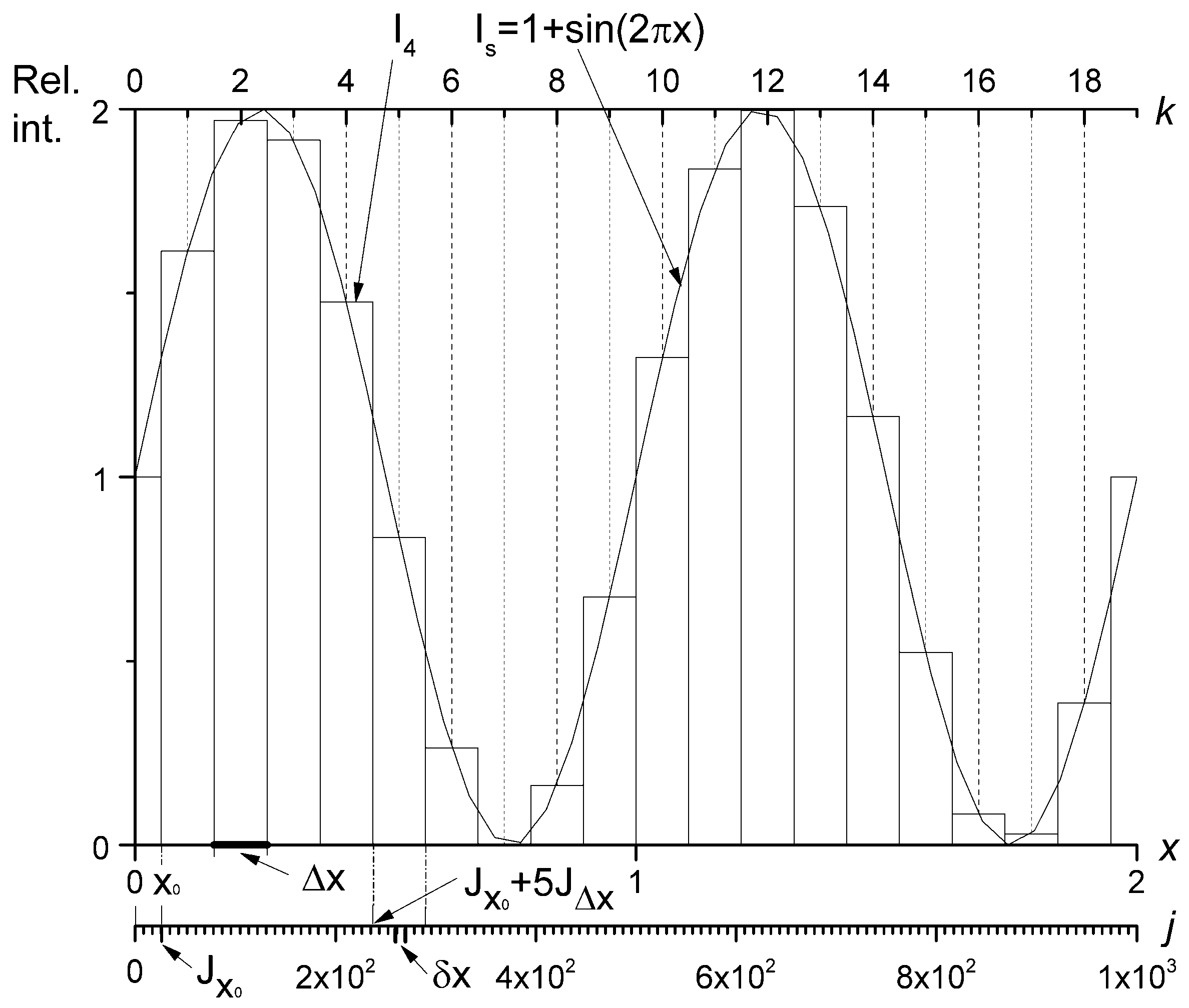
The output value recorded by the detector at the position of the k-th pixel of a size $\Delta x$ can be described by:

$$I_k\left(x_0+k\Delta x\right)=1+\frac{1}{J_{\Delta x}}{\displaystyle \sum }_{j_{k-1}}^{j_k}\sin \left[2\pi \left(x_0+j\delta x\right)\right]$$

(4)

where the summation limits are $j_{k-1}=J_{x_0}+\left(k-1\right)J_{\Delta x}$ and $j_k=J_{x_0}+k{J}_{\Delta x}$, and where $J_{x_0}$ is the total number of calculation points describing the phase shift of the detector regarding the fixed input sinusoidal signal. Thus, the output pattern has constant values across each pixel area $k\Delta x$ for the total of K pixels. This concept is illustrated in Figure 2.

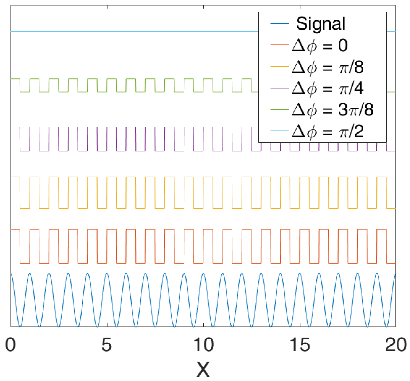
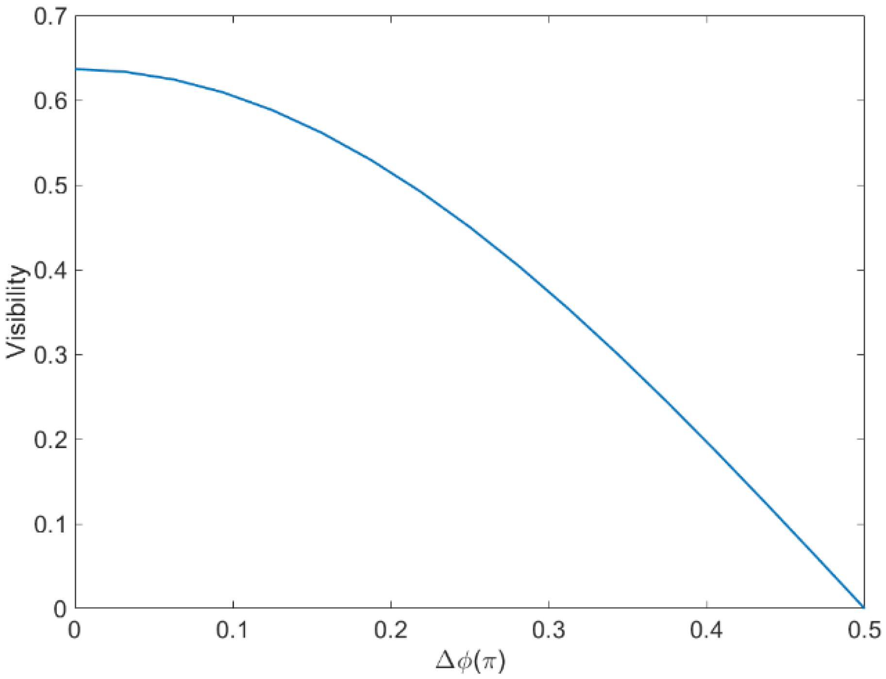
In Figure 3, the input signal is sampled under the Nyquist condition, where the effect of phase shifts between PCD pixels and the input signal is shown. The sine curve (the lowest one) represents the input signal to the detector, Equation (3), while other lines are readout signals acquired and digitized by the detector for the following $\Delta \phi =2\pi x_0$ values, $\Delta \phi =0, \pi /8, 2\pi /8, 3\pi /8, 4\pi /8$. As it can be expected, for $\Delta \phi =\pi /2$, the recorded pattern becomes flat. Therefore, a complete loss of visibility is possible under Nyquist conditions. Figure 4 shows the dependence of the fringe visibility function on the phase shift at the Nyquist frequency.

Since we generally have two spatial frequencies involved, one defined by the input pattern, $f_0=1/X$, and the other defined by the detector’s pixel size, $f=1/\left(2\Delta x\right)$, the beating effect occurs as demonstrated in DH previously [26]. In our case, the beating can be observed for

$$\left|2\Delta x-X\right|=\epsilon x, \epsilon x\ll 2\Delta x, X; \epsilon x\ne 0$$

(5)

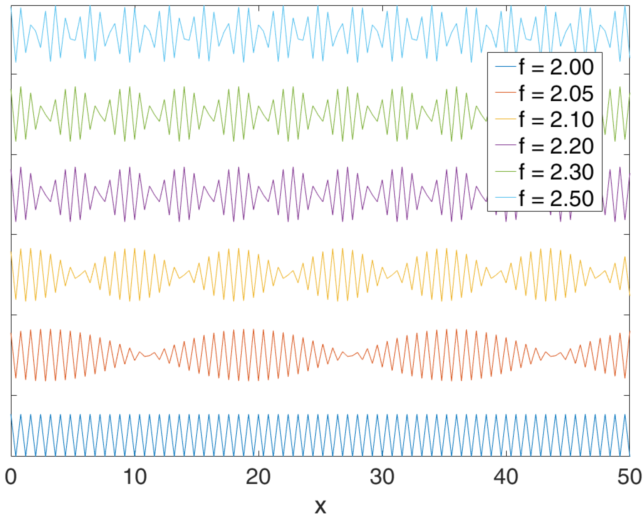
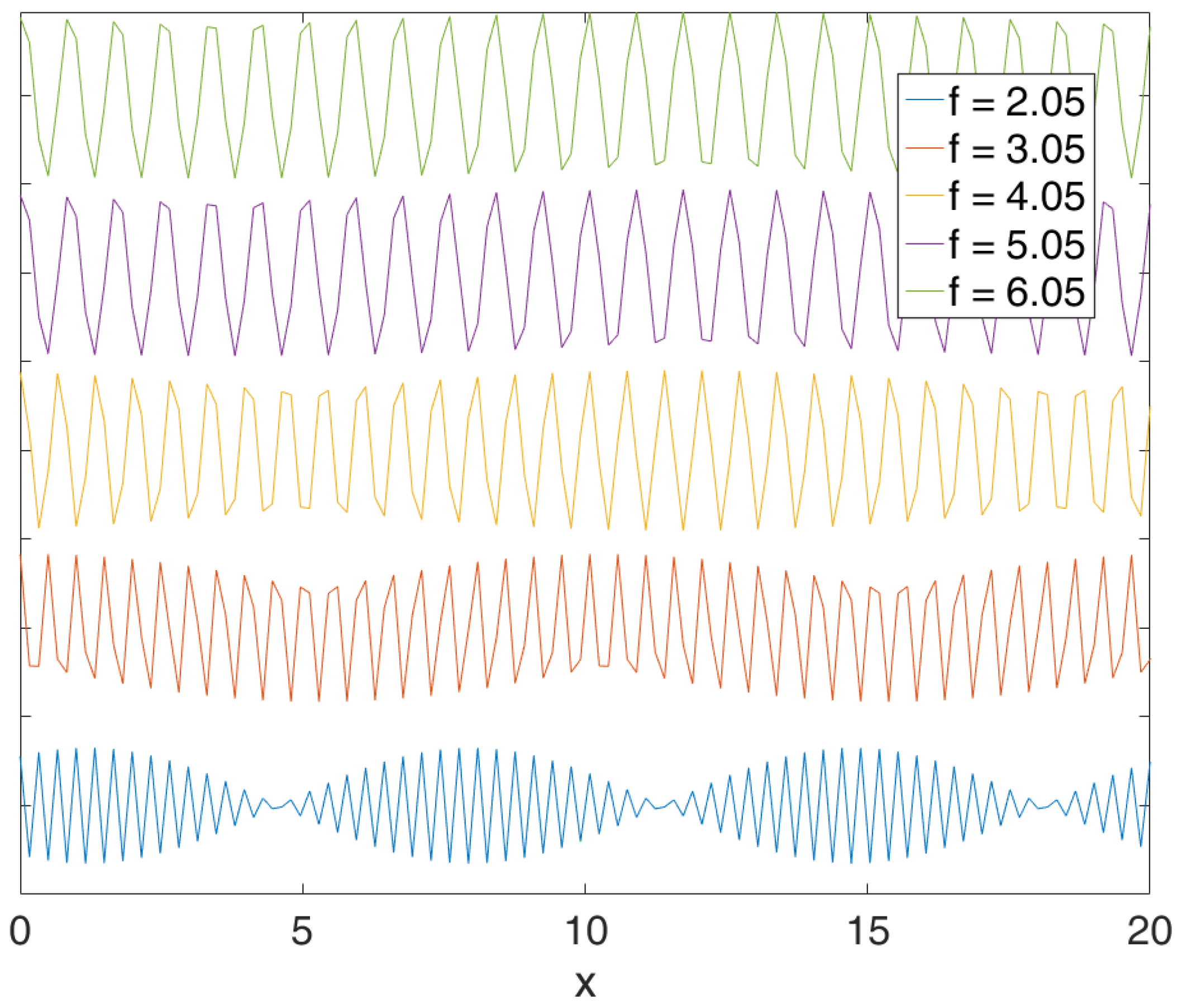
where $\epsilon x$ is the absolute value of the difference between the period of the sinusoidal input pattern and the period defined by the detector’s Nyquist condition. Thus, the readout signal is modulated by the beating frequency $f_B=\left|f-f_0\right|$ with a period $T_B=2\Delta xX/\epsilon x$. This effect is illustrated in Figure 5, where the recorded signal is calculated for several sampling frequencies f, near Nyquist frequency (f_N = 2). Changing f in simulations means that the pixel size of the detector is changing. From Figure 5, it can be seen that the highest beating amplitude occurs when the input signal and the detector’s pixel are in phase. Also, note that some of the patterns depicted in Figure 5 resemble patterns in the recorded hologram, shown in Figure 1. Of course, with the increase of the sampling rate, the beatings fade out. Figure 6 shows a decrease in the beating effect for higher frequencies ($f\ge 2.5 f_N$).

The local fringe visibility at the k-th pixel, $V\left(x_0+k\Delta x\right)$ can be calculated according to Equation (2) for two subsequent output intensity values. To measure the quality of the recorded pattern, we calculate the local signal-to-noise ratio (SNR) as:

$$SNR\left(k,j\delta x\right)=\frac{V\left(x_0+k\Delta x\right)}{{\left\{\frac{1}{J_{\Delta x}}{{\displaystyle \sum }}_{j=j_{k-1}}^{j_k}{\left[I_S\left(j\delta x\right)-I_k\left(x_0+k\Delta x\right)\right]}^2\right\}}^{1/2}}$$

(6)

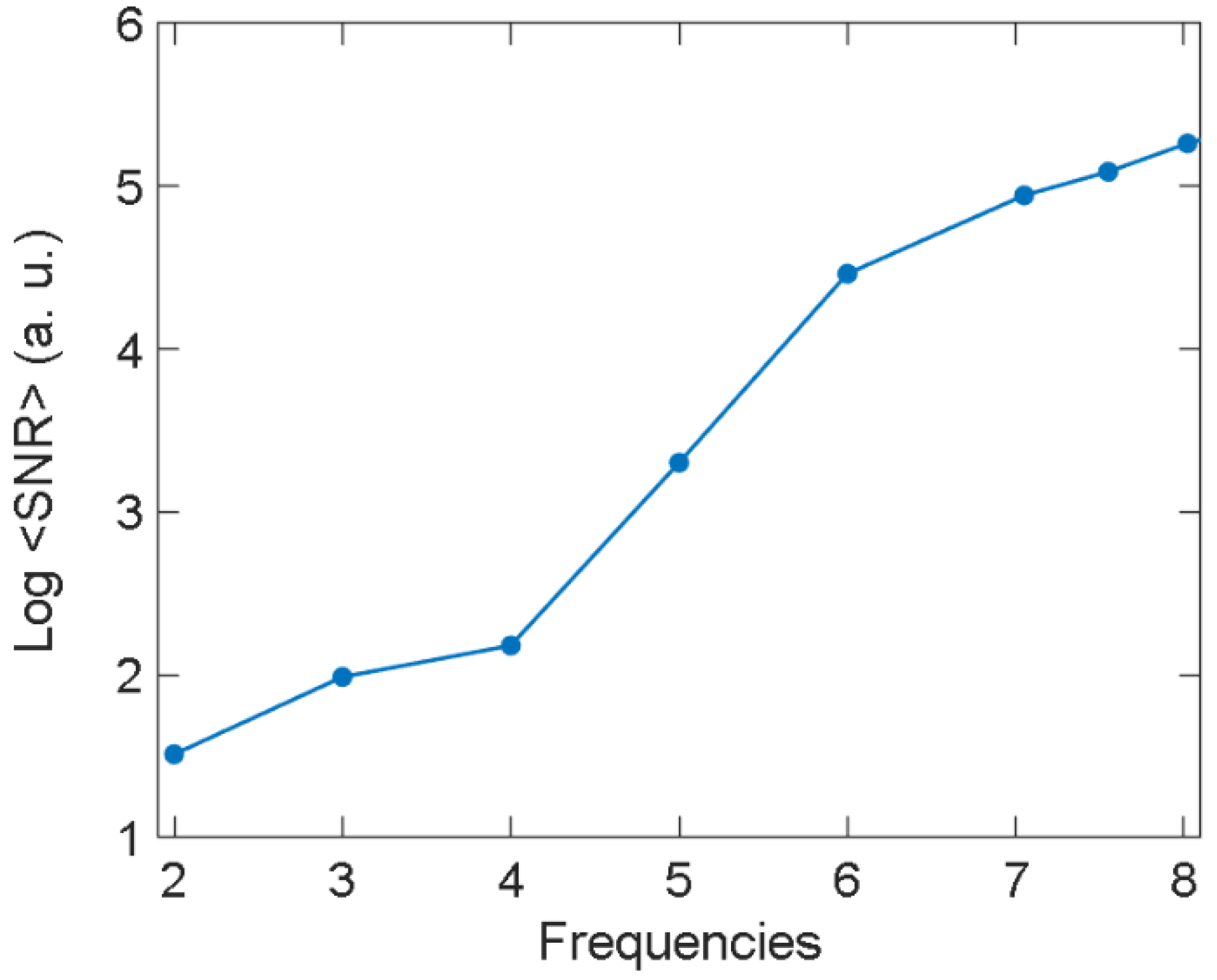
In Equation (6), the numerator is calculated according to Equation (2) and can take values between 0 and 1. The denominator is standard deviation, i.e., the square root of the average of the squared differences between the ideal sinusoidal signal described by Equation (3) and the output constant value detected at the position $\left(x_0+k\Delta x\right)$. In typical calculations, by taking at least 10 points per pixel size $\Delta x$, the standard deviation will always have some finite value greater than zero. Theoretically, the SNR can be indeterminate for an infinitesimally small pixel size ($\Delta x\to 0, SNR=0/0$) but such a situation cannot be realized in reality. The SNR values averaged over a period are shown in Figure 7, where it is evident that considerable rise is achieved for sampling frequencies above $f=2.5 f_N$.

The purpose of this section is to highlight the loss of information that occurs in the image plane DHM when holograms are recorded near the Nyquist frequency. We have simulated detection of an ideal sinusoidal pattern by a one-dimensional array which has the possibility of shifting and changing its pixel size. The patterns with beating effects (Figure 4 and Figure 5) are clearly shown, and the conditions for forming such patterns have been presented. The similarity of patterns in Figure 5 and the recorded hologram in Figure 1 is well established. Since the beating effect inevitably causes loss of information, an optimum sampling rate (i.e., optimum detector’s pixel size) should be estimated to avoid both beating and redundancy. The results shown in Figure 6 and Figure 7 may serve as a useful guide in setting the optimum frequency in practical setups. We have estimated the optimum frequency as $f=2.5 f_N$ and applied that value in a practical study.

2.2. Experimental Setup

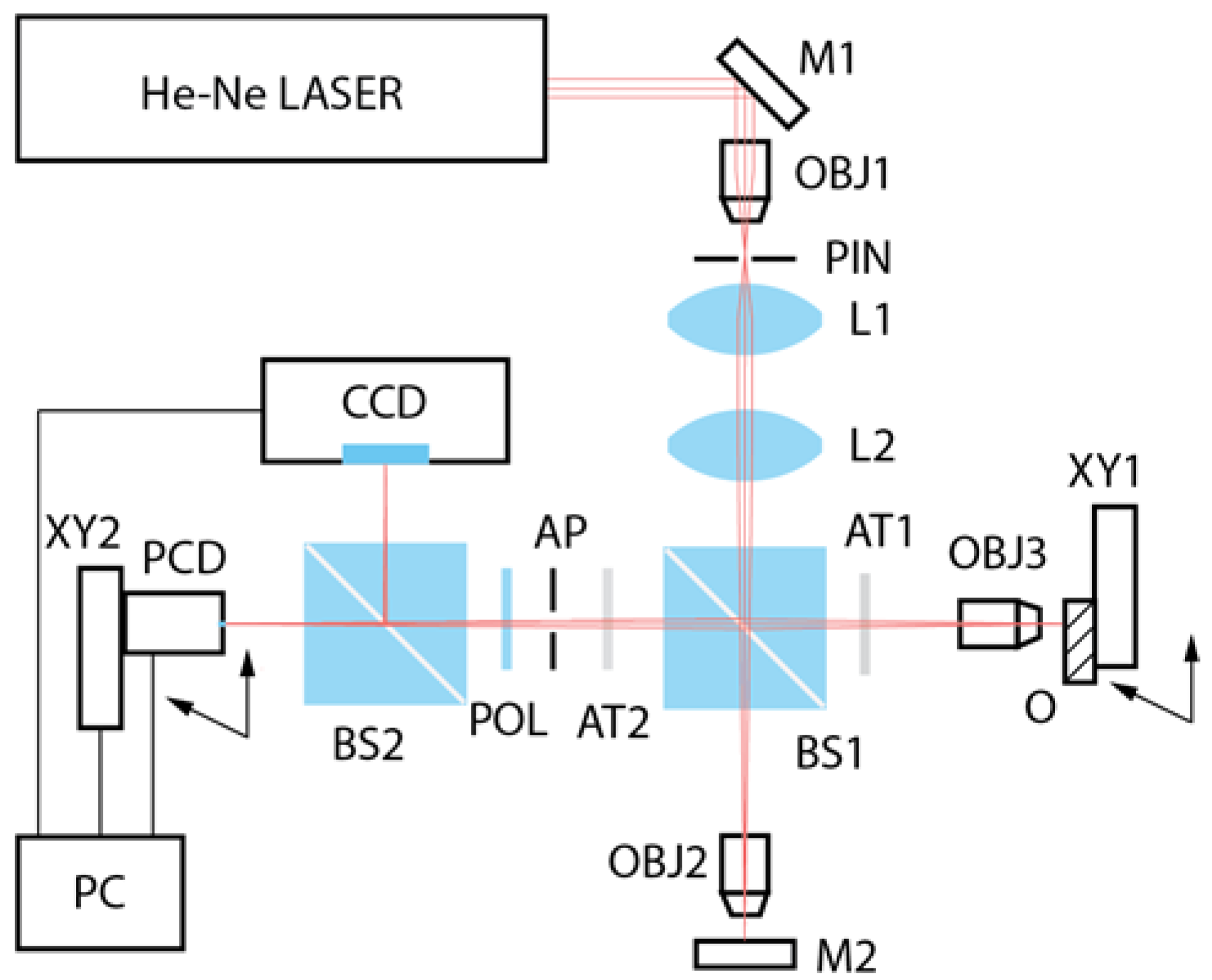
Figure 8 illustrates the experimental setup employed for all measurements. The used setup is a Twyman-Green interferometer with He-Ne laser (wavelength 632.8 nm) as a light source. Before entering the interferometer, the laser beam is spatially filtered by a microscope objective (40× magnification) and a pinhole (10 μm). After the spatial filtering, the beam is collimated by the first lens (100 mm) and slightly focused by the second lens (300 mm). Inside the interferometer on both sides are two equal microscope objectives (10× magnification). The object and the reference mirror (M2, λ/10 flatness) are tilted with respect to each other (not depicted on the scheme) to provide a certain spatial frequency of fringes. Manual XY translation stage (XY1) holds an object (O). For adjusting the intensity ratio of the reference to the object beam, various neutral density filters (AT1-2) are used. Two detectors, a CCD camera (Imperx IPX-4M15), and a PCD mounted on a motorized XY translation stage are located at the same distance from the object. We used the best available (regarding the signal-to-noise ratio) CCD camera with an active area of 16.67 × 16.05 mm², pixel size of 7.4 μm and full well capacity is 40,000 electrons. The PCD is a homemade one, based on a single-photon avalanche photodiode (SPAD) (model SAP500, LC) selected for low noise, cooled to −23 °C, and operated in Geiger mode. The detector features a maximum count rate of 10 Mcps and a dark count rate of 21 cps; for more details, see [27]. A small aperture was placed before the SPAD to increase the resolution. We used apertures of 1 μm and 2 μm which determined the resolution. Hologram recordings are made with the PCD during motorized movement of the translation stage. Thus, the pixel size is defined by the product of the speed at which the PCD moves and the integration time convoluted with the aperture size. Each line of a hologram was taken separately, always in the same direction, and during the transition to the next line, the recording was stopped. The maximum size of holograms taken with moving PCD was 3000 × 3000 pixels, and the recording time was 6 h. For smaller sizes, the recording time was shorter. The CCD camera recordings are used for comparison.

3. Results

For comparing the linearity of holograms captured by the CCD and the PCD, we used the 1951 USAF resolution target. We then applied the optimum sampling analysis and photon-counting approach to study the thin metallic film buckling.

3.1. Nonlinear Recording

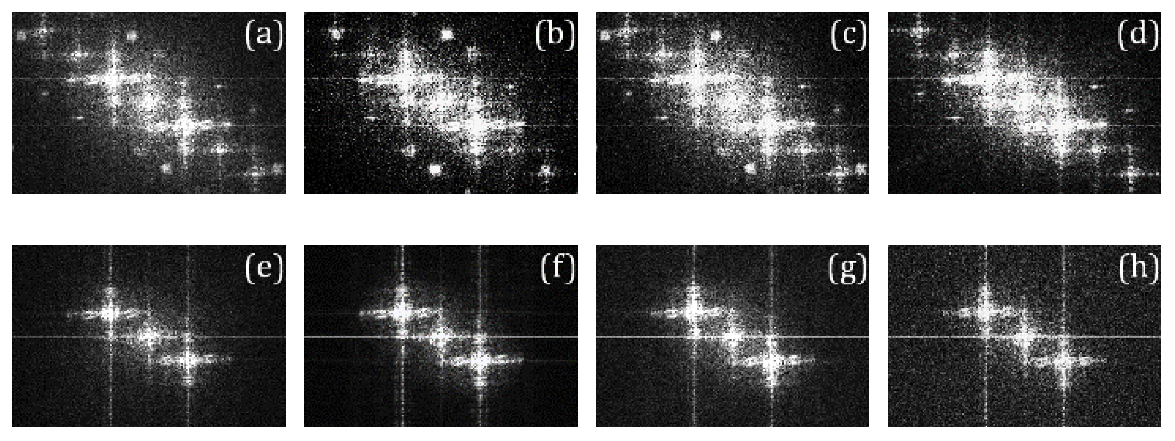
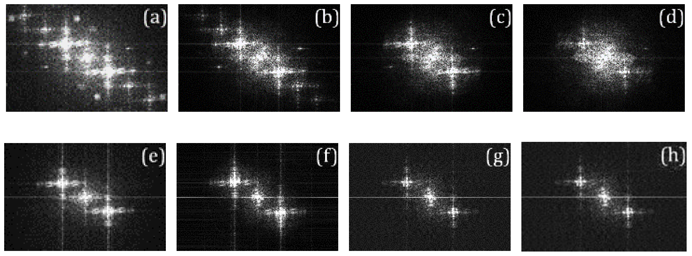
The linearity is best indicated in the Fourier domain since the first-order term is linear characteristics of the response, while the higher terms represent nonlinearities. Nonlinear recording of sinusoidal patterns is difficult to avoid by standard array detectors. Since the nonlinearity is best revealed in the frequency domain, we show the Fourier transform (FT) spectra of the recorded holograms. We compared the linearity of the recorded holograms obtained by the CCD sensor and the PCD in a Twyman-Green setup shown in Figure 8. For this analysis, the off-axis angle is chosen to be far from the Nyquist limit, and all experimental conditions are kept identical for the measurements to be compared. It should be noted that the acquisition time of the DHs recorded by the CCD is much shorter than the acquisition time of the corresponding DHs recorded by the PCD. The obtained results for various experimental conditions are presented in Figure 9 and Figure 10. First, the DHs are recorded by attenuating both the reference and the object beams by the same neutral density (ND) filter while adequately prolonging the exposure time of the DHs. Second, we repeated the procedure by attenuating only the object beam. The upper row of Figure 9 and Figure 10 (the CCD DHs) should be compared with the corresponding bottom row (PCD DHs). All PCD DHs have demonstrated linear recording even in considerably noisy conditions. As expected, the CCD DHs have shown linear recording only for higher reference to object beam intensity ratios (Figure 10c,d).

3.2. Thin Metallic Filmbuckling

As a model for testing hologram recording in DHM configuration with moving PCD, the thin film buckling structures were used. The topography of buckling patterns that can be observed on thin film during or after its delamination from thick substrate has been of considerable interest [28,29,30]. For deposition of tungsten thin films by magnetron sputtering, it is known that argon pressure significantly affects film internal stress. In the case of tensile residual stress, a network of through-thickness cracks forms in the film while the residually compressed thin films may delaminate from substrate and buckle. The buckling of thin tungsten film can result in several topographical patterns such as disordered surface wrinkles, regular herringbone, straight-sided or telephone cord buckles, and circular blisters. The associated mechanics have been studied for all types of buckles, but for the telephone cord (TC), more precise microscopic observation (complemented by topographic measurements) is still needed for testing the corresponding models [31]. In general, buckling profiles can be characterized depending on scale, by mechanical or laser-scanning profilometry, optical interferometer microscopy, or by using an atomic force microscope [31,32]. These objects were chosen because of their well-defined surface, stability over time, and reflectivity that was not too low. As already indicated, maximum care was taken to make the whole setup the most stable since the scanning procedure lasts long. For holograms presented here, we took 3000 × 3000 pixels which lasted about six hours per hologram.

The DHs were recorded by first employing the setup shown in Figure 8 and then reconstructed by a standard procedure for several topological structures. The fundamental fringe period, defined by the angle between the object and the reference beam, was around 17 μm, and the scanning step was chosen to be 3 μm according to the optimal sampling analysis. The standard numerical procedure for reconstructing image plane DHs can be described briefly as: (i) the recorded DH is Fourier transformed yielding for linear recordings three separated terms (zeroth, plus first, and minus first orders) in the frequency plane, (ii) one diffraction term (for example, plus first) is isolated, (iii) the resulting image with the isolated part is inverse Fourier transformed, and (iv) the obtained image is multiplied by its complex conjugate. Alternatively, the same procedure can be performed by optical means using a high-resolution liquid crystal display [33].

Along with the reconstruction of DHs, we calculated interferograms which helped us reveal the topological information about film buckling from a single recorded hologram. The interferograms were calculated by the following procedure. In the first step, the background hologram was numerically produced from the original hologram. The background should emulate the hologram of the surface without the object. For this procedure, it is important that a well-defined surface exists outside of the object. Each hologram consists of N horizontal lines, and each line is M pixels long. Every j-th line is represented with a simple cosine function in the form:

$$y_j\left(i\right)=A_{j }+B_{j }\cos \left(f_{x }i+{\delta }_{j }\right),\hspace{1em}i=1,2,\dots M,\hspace{1em}j=1,2,\dots N$$

(7)

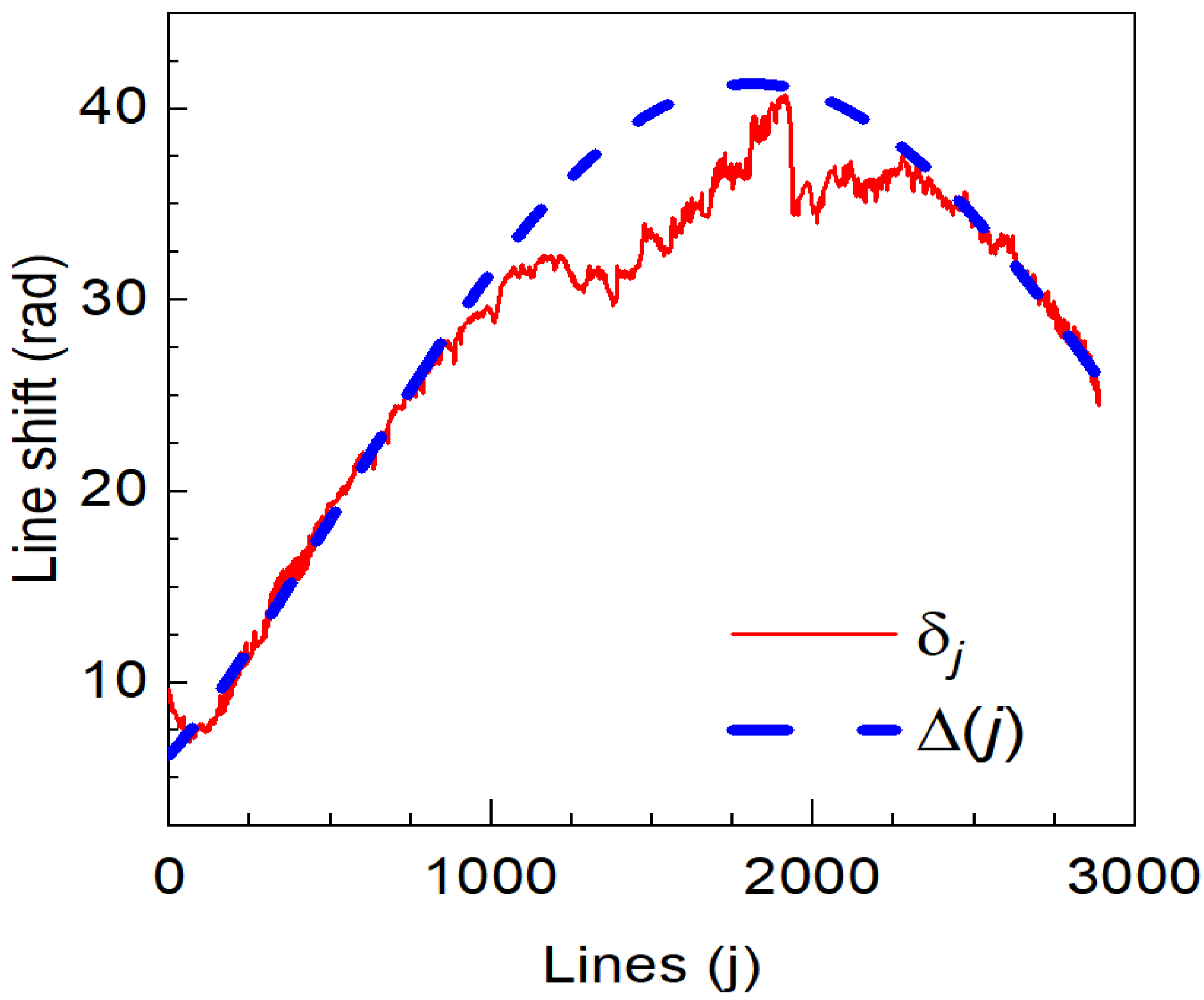
The fundamental fringe frequency, f_x, assumed to be the same for every line, is deduced from simple Fourier analysis. Then each line j is fitted separately one after another with fitting parameters: A_j the offset, B_j the amplitude, and δ_j the fundamental fringe shift of the line. For the start value regarding fitting the specific δ_j, the previous value, δ_j−1 is taken. In this way, we avoid the phase jumps and obtain δ_j value for each line. These values are smooth along the lines, except maybe at the region where the object is located. The overall smooth function of the shift, ∆(j), is then retrieved from the fitting of the δ_j for j = 1, 2, …, N. In this fitting procedure, more weight is given to the lines on the edges, i.e., the regions of the hologram outside the object. An example of finding ∆(j) as polynomial $\Delta \left(j\right)={\displaystyle \sum }_{k=0}^4{c}_k j^k$ is shown in Figure 11.

As can be seen, the smooth function fits almost perfectly the fringe shifts outside of the object. Finally, the background BH(i, j) was constructed as:

$$BH\left(i,j\right)={\displaystyle \sum }_j^M{\displaystyle \sum }_i^N\left[AA+BB \cos (f_{x}i+\Delta \left(j\right)\right]$$

(8)

where $AA={\displaystyle \sum }_{j=1}^M{A}_j/M$, and $BB={\displaystyle \sum }_{j=1}^M{B}_j/M$ are mean values of the offset and the amplitude, respectively, and their values are not so important for the procedure. Then the background was subtracted from the hologram and reconstructed.

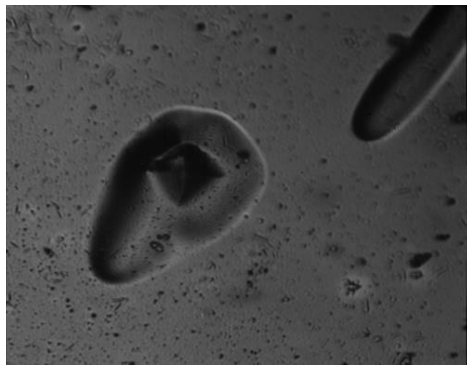
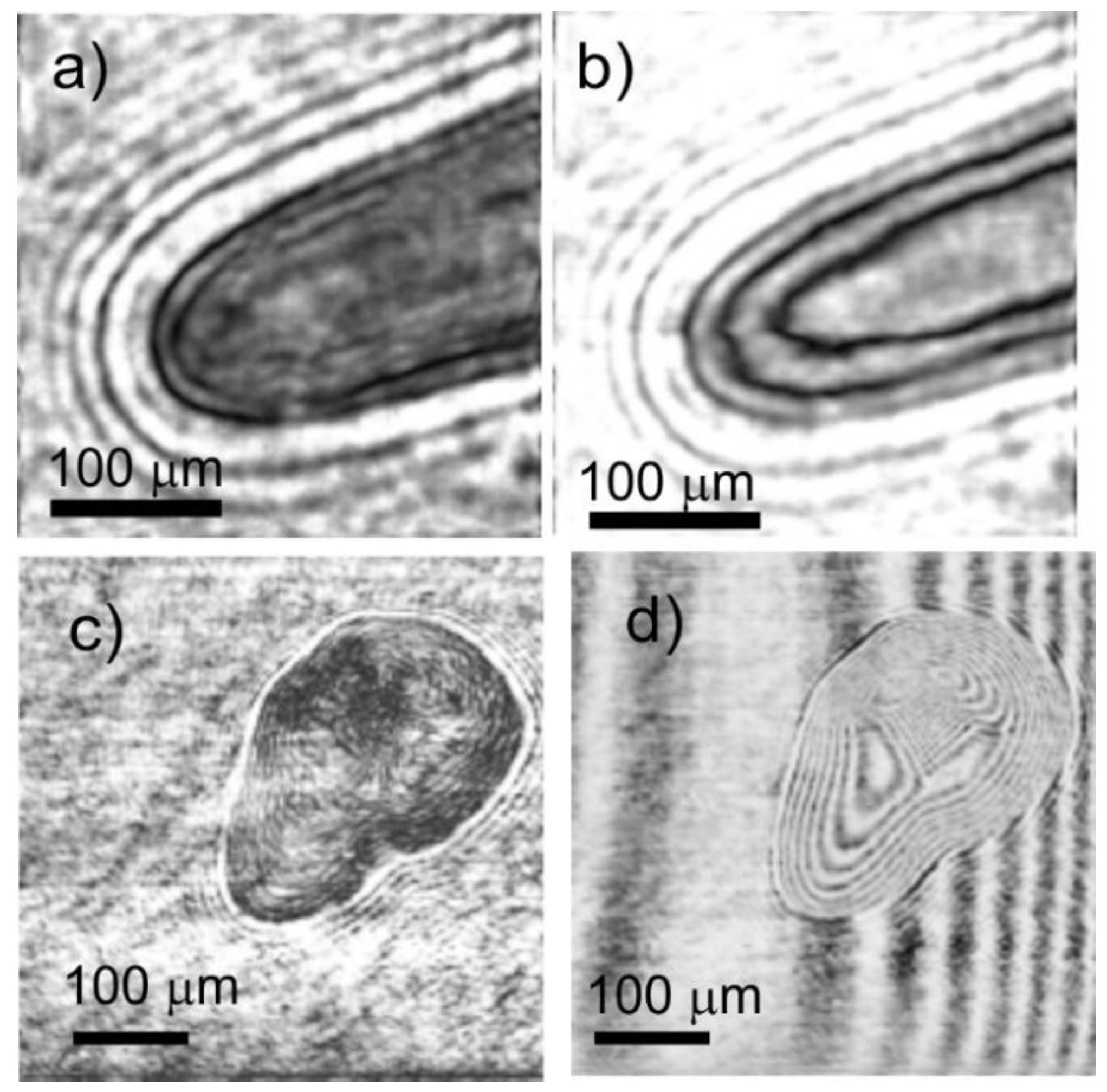
We demonstrate our approach by recording holograms of two objects that appear on the tungsten 4 μm thin film originally deposited by magnetron sputtering on a glassy substrate. The first object is a tip of the straight-line delamination buckling type structure formed by an in situ thermal gradient. The second buckling structure has been developed after poking the flat area by Vickers indentor (100 N force) due to local relaxation of the residual stress in the same thin film. Both of these two structures are shown by white-light microscopy in Figure 12.

The holographic analysis of the buckling and the blister is illustrated in Figure 13. The left columns in Figure 13 show amplitude reconstruction from holograms, obtained by the usual procedure. The right-hand side of Figure 13b–d are reconstructions of the interferograms generated by the above-mentioned method. The fringes which can be seen depict the iso-lines of the topological structure of those two microscopic objects, thus yielding obvious qualitative information of height distribution of the object.

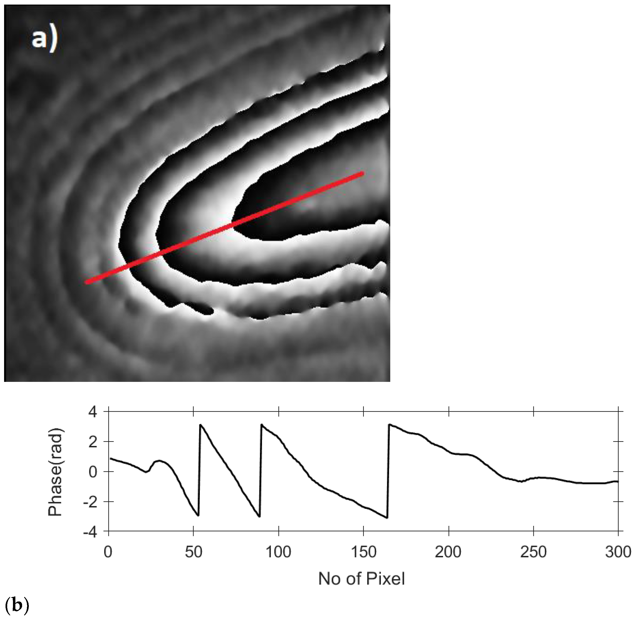
Quantitative information can be extracted from the phase, which is wrapped in the steps of 2π. There are many unwrapping algorithms described in the literature [34], but the core idea is to find true phase values and then map these values to the object height. In Figure 14a, we illustrate the modulo 2π phase distribution and the corresponding line profile in Figure 14b.

4. Discussion

Typically, holograms are recorded close to saturation to obtain large SNR. For hologram recording, this means that nonlinearities are often unavoidable. The presence of terms above the first-order in the Fourier domain, such as in Figure 9a–d and Figure 10a,b, indicate saturation in a digital recording of holograms. The signal recorded with a CCD camera is constrained by a limited dynamic range (mostly 256 gray levels). However, when using PCD as a recording device, the signal is always unsaturated, as shown in corresponding figures, e.g., Figure 9e–h and Figure 10e,f.

Although the values of the experimental parameters have been arbitrarily chosen, the obtained results are consistent concerning the linearity issue. We remark that when the hologram is recorded by the CCD in attenuated conditions, it would be possible to some extent to eliminate nonlinearities while having low noise by summing holograms to the same number of photons as acquired in a single hologram. We cannot say that a scanning PCD is a better solution than CCD or CMOS cameras, but fast emerging new devices based on an array of photon-counting photodiodes should show benefits in holography regarding linearity issues.

The issue with optimum sampling was studied with scanning PCD inserted in the Twyman-Green optical setup (shown in Figure 8) and used for recording digital holograms. As an input object, we used a stable structure of buckling patterns on tungsten thin film. We followed the procedure presented in Section 2.1 by, first by finding the Nyquist frequency and then by taking the spatial frequency 2.5 times the Nyquist frequency for recording digital holograms. To find the topology of objects from a single recorded hologram, we utilized the numerical procedure described in Section 3.2. The obtained results demonstrate successful recording of digital holograms as well as useful production of synthetic interferograms. Figure 13d shows smooth interferometric fringes describing most of the topology of the blister accurately. The area of low contrast fringes corresponds to the very steep slope of the blister.

We have demonstrated a method for recording perfectly linear and optimum sampled digital holograms particularly suited for efficient use of a PCD in the image plane DHM configurations. Aside from the general problem in the DHM of nonlinear hologram recording, image plane configurations are often suffering from inadequate sampling regarding the information content (undersampled or oversampled holograms). Namely, for holograms recorded near the Nyquist sampling rate, the frequency beatings occur due to the slight local phase shifts leading to a loss of hologram information. An obvious approach to increasing the sampling frequency to a safety zone (far above the Nyquist rate) is not always possible. To overcome that problem, we found an optimized sampling measure through numerical analysis and applied it in a practical DHM system. The PCD was mounted on a motorized XY translation stage, which enabled flexibility in changing the pixel size of the hologram recording (product of the speed at which the PCD moves and the integration time). Thus, by employing the PCD, hologram recordings were inherently linear, and the sampling rate was easily adjusted to an optimized value. Currently, this approach is feasible for stable measuring conditions and static objects because of long recording times. However, the presented work can be useful in future optimal use of more advanced PCD based systems for hologram recordings in the image plane DHM. This includes phase measurements not only of technical microstructures (particularly suitable are test structures obtained by 3D printing), but also of biological and biomedical specimens, as detailed in article reviews [35,36]. We emphasize the holographic tomography applications with beam rotation or sample rotation architectures, where variations in both the spatial frequency and beam ratio must be optimized, which our method offers.

References

- Kim, M.K. Digital Holographic Microscopy; Springer Series in Optical Sciences; Springer: New York, NY, USA, 2011; Volume 162, ISBN 978-1-4419-7792-2. [Google Scholar]
- Anand, A.; Chhaniwal, V.; Javidi, B. Tutorial: Common path self-referencing digital holographic microscopy. APL Photon. 2018, 3, 071101. [Google Scholar] [CrossRef]
- Bishara, W.; Su, T.-W.; Coskun, A.F.; Ozcan, A. Lensfree on-chip microscopy over a wide field-of-view using pixel super-resolution. Opt. Express 2010, 18, 11181. [Google Scholar] [CrossRef] [PubMed]
- Serabyn, E.; Liewer, K.; Lindensmith, C.; Wallace, J.; Nadeau, J. Compact, lensless digital holographic microscope for remote microbiology. Opt. Express 2016, 24, 28540. [Google Scholar] [CrossRef] [PubMed]
- Singh, M.; Khare, K. Single-shot full resolution region-of-interest (ROI) reconstruction in image plane digital holographic microscopy. J. Mod. Opt. 2018, 65, 1127. [Google Scholar] [CrossRef]
- Goodman, J.W. Speckle Phenomena in Optics Theory and Applications; Roberts and Company: Englewood, CO, USA, 2007; ISBN 978-1-9362-2114-1. [Google Scholar]
- Bianco, V.; Memmolo, P.; Leo, M.; Montresor, S.; Distante, C.; Paturzo, M.; Picart, P.; Javidi, B.; Ferraro, P. Strategies for reducing speckle noise in digital holography. Light. Sci. Appl. 2018, 7, 48. [Google Scholar] [CrossRef] [PubMed]
- Charriére, F.; Rappaz, B.; Kühn, J.; Colomb, T.; Marquet, P.; Depeursinge, C. Influence of shot noise on phase measurement accuracy in digital holographic microscopy. Opt. Express 2007, 15, 8818. [Google Scholar] [CrossRef]
- Monaldi, A.C.; Romero, G.G.; Cabrera, C.M.; Blanc, A.V.; Alanís, E.E. Rolling Shutter Effect aberration compensation in Digital Holographic Microscopy. Opt. Commun. 2016, 366, 94. [Google Scholar] [CrossRef]
- Remmersmann, C.; Stürwald, S.; Kemper, B.; Langehanenberg, P.; Von Bally, G. Phase noise optimization in temporal phase-shifting digital holography with partial coherence light sources and its application in quantitative cell imaging. Appl. Opt. 2009, 48, 1463. [Google Scholar] [CrossRef]
- Bothe, T.; Burke, J.; Helmers, H. Spatial phase shifting in electronic speckle pattern interferometry: Minimization of phase reconstruction errors. Appl. Opt. 1997, 36, 5310. [Google Scholar] [CrossRef]
- Styk, A.; Patorski, K. Identification of nonlinear recording error in phase shifting interferometry. Opt. Lasers Eng. 2007, 45, 265. [Google Scholar] [CrossRef]
- Pan, B.; Kemao, Q.; Huang, L.; Asundi, A. Phase error analysis and compensation for nonsinusoidal waveforms in phase-shifting digital fringe projection profilometry. Opt. Lett. 2009, 34, 416. [Google Scholar] [CrossRef] [PubMed]
- Cywińska, M.; Trusiak, M.; Zuo, C.; Patorski, K. Enhancing single-shot fringe pattern phase demodulation using advanced variational image decomposition. J. Opt. 2019, 21, 045702. [Google Scholar] [CrossRef]
- Claus, D.; Iliescu, D.; Bryanston-Cross, P. Quantitative space-bandwidth product analysis in digital holography. Appl. Opt. 2011, 50, H116. [Google Scholar] [CrossRef] [PubMed] [Green Version]
- Onural, L. Sampling of the diffraction field. Appl. Opt. 2000, 39, 5929. [Google Scholar] [CrossRef] [PubMed] [Green Version]
- Demoli, N.; Halaq, H.; Sariri, K.; Torzynski, M.; Vukicevic, D. Undersampled digital holography. Opt. Express 2009, 17, 15842. [Google Scholar] [CrossRef]
- Demoli, N.; Meštrović, J.; Sovic, I. Subtraction digital holography. Appl. Opt. 2003, 42, 798. [Google Scholar] [CrossRef]
- Leclercq, M.; Picart, P. Digital Fresnel holography beyond the Shannon limits. Opt. Express 2012, 20, 18303. [Google Scholar] [CrossRef]
- Tahara, T.; Awatsuji, Y.; Nishio, K.; Ura, S.; Matoba, O.; Kubota, T. Space-Bandwidth Capacity-Enhanced Digital Holography. Appl. Phys. Express 2013, 6, 22502. [Google Scholar] [CrossRef] [Green Version]
- Agbana, T.E.; Gong, H.; Amoah, A.S.; Bezzubik, V.; Verhaegen, M.; Vdovin, G. Aliasing, coherence, and resolution in a lensless holographic microscope. Opt. Lett. 2017, 42, 2271. [Google Scholar] [CrossRef] [Green Version]
- Yamamoto, M.; Yamamoto, H.; Hayasaki, Y. Photon-counting digital holography under ultraweak illumination. Opt. Lett. 2009, 34, 1081. [Google Scholar] [CrossRef]
- Demoli, N.; Skenderović, H.; Stipčević, M. Digital holography at light levels below noise using a photon-counting approach. Opt. Lett. 2014, 39, 5010. [Google Scholar] [CrossRef]
- Demoli, N.; Skenderović, H.; Stipčević, M. Time-averaged photon-counting digital holography. Opt. Lett. 2015, 40, 4245. [Google Scholar] [CrossRef]
- Wallace, J.K.; Rider, S.; Serabyn, E.; Kühn, J.; Liewer, K.; Deming, J.; Showalter, G.; Lindensmith, C.; Nadeau, J.L. Robust, compact implementation of an off-axis digital holographic microscope. Opt. Express 2015, 23, 17367. [Google Scholar] [CrossRef] [Green Version]
- Demoli, N. Real-time monitoring of vibration fringe patterns by optical reconstruction of digital holograms: Mode beating detection. Opt. Express 2006, 14, 2117. [Google Scholar] [CrossRef]
- Stipčević, M.; Skenderović, H.; Gracin, D. Characterization of a novel avalanche photodiode for single photon detection in VIS-NIR range. Opt. Express 2010, 18, 17448. [Google Scholar] [CrossRef] [Green Version]
- Freund, L.B.; Suresh, S. Thin Film Materials; Cambridge University Press: Cambridge, MA, USA, 2003; pp. 86–153. ISBN 978-0-5215-2977-8. [Google Scholar]
- Mondal, K.; Liu, Y.; Shay, T.; Genzer, J.; Dickey, M.D. Application of a Laser Cutter to Pattern Wrinkles on Polymer Films. ACS Appl. Polym. Mater. 2020, 2, 1848. [Google Scholar] [CrossRef]
- Tang, J.; Qiu, Z.; Li, T. A novel measurement method and application for grinding wheel surface topography based on shape from focus. Measurement 2019, 133, 495. [Google Scholar] [CrossRef]
- Faou, J.-Y.; Parry, G.; Grachev, S.; Barthel, E. How Does Adhesion Induce the Formation of Telephone Cord Buckles? Phys. Rev. Lett. 2012, 108, 116102. [Google Scholar] [CrossRef]
- Moon, M.; Jensen, H.; Hutchinson, J.; Oh, K.; Evans, A. The characterization of telephone cord buckling of compressed thin films on substrates. J. Mech. Phys. Solids 2002, 50, 2355. [Google Scholar] [CrossRef]
- Demoli, N.; Halaq, H.; Vukicevic, D. White light reconstruction of image plane digital holograms. Opt. Express 2010, 18, 12675. [Google Scholar] [CrossRef]
- Zappa, E.; Busca, G. Comparison of eight unwrapping algorithms applied to Fourier-transform profilometry. Opt. Lasers Eng. 2008, 46, 106. [Google Scholar] [CrossRef]
- Park, Y.; Depeursinge, C.; Popescu, G. Quantitative phase imaging in biomedicine. Nat. Photon. 2018, 12, 578. [Google Scholar] [CrossRef]
- Balasubramani, V.; Kujawińska, M.; Allier, C.; Anand, V.; Cheng, C.-J.; Depeursinge, C.; Hai, N.; Juodkazis, S.; Kalkman, J.; Kuś, A.; et al. Roadmap on Digital Holography-Based Quantitative Phase Imaging. J. Imaging 2021, 7, 252. [Google Scholar] [CrossRef] [PubMed]
Figure 1.
Image plane hologram of the 1951 USAF resolution target recorded using the experimental setup described in Section 3. The inset shows the signal along one line of the hologram.
Figure 2.
The concept used for numerical simulations (as described in the text).
Figure 3.
Numerical model of the signal digitization at Nyquist frequency. The lowest curve represents the original signal, the other curves from the bottom to the top are recordings for the phase shifts 0, π/8, π/4, 3π/8, and π/2.
Figure 4.
Fringe visibility at Nyquist frequency as a function of the phase.
Figure 5.
The beating effect shown for the sampling frequencies around Nyquist frequency. The graphs show signals for f = 2.00, 2.05, 2.10, 2.20, 2.30, and 2.50 (from the bottom to the top).
Figure 6.
The signals for the sampling frequencies above Nyquist show a decrease in beatings. From the bottom to the top: f = 2.05, 3.05, 4.05, 5.05, and 6.05.
Figure 7.
The average SNR vs. sampling frequency in the lin-log scale.
Figure 8.
Twyman-Green experimental setup. He-Ne, Helium-neon; M1and M2, mirrors; OBJ1-3, microscope objectives; PIN, pinhole; L1 and L2, lenses; BS1-2, beam splitters; AT1-2, neutral density filters; O, object; POL, polarizer; AP, aperture; PCD, single-photon counting detector; XY1, manual translation stage; and XY2, motorized translation stage.
Figure 9.
(a–d): FT spectra recorded with CCD using ND filters on both beams with OD = 0, 1.0, 2.0 and 3.0, respectively. (e–h): FT spectra recorded with PCD using ND filters on both beams with OD = 0, 1.0, 2.0 and 3.0, respectively.
Figure 10.
(a–d): FT spectra recorded with CCD using ND filters to attenuate the object beam with OD = 0, 0.6, 1.3, and 2.0, respectively. (e–h): FT spectra recorded with PCD using ND filters to attenuate the object beam with OD = 0, 0.6, 1.3, and 2.0, respectively.
Figure 11.
Fitting of δj for an object located between lines 1000 and 2500.
Figure 12.
Microscopic image of a blister and a tip of a filmbuckling structure.
Figure 13.
Object reconstruction from the hologram (a,c), and object reconstruction from the interferogram (b,d). Pictures (a,b) depict the end of the telephone cord buckle, and (c,d) depict a poke in the thin film that caused inflation of the structure.
Figure 14.
(a): Phase picture of the object shown in Figure 13b, and (b): phase values along the red line.
Publisher’s Note: MDPI stays neutral with regard to jurisdictional claims in published maps and institutional affiliations. |
© 2022 by the authors. Licensee MDPI, Basel, Switzerland. This article is an open access article distributed under the terms and conditions of the Creative Commons Attribution (CC BY) license (https://creativecommons.org/licenses/by/4.0/).
Share and Cite
MDPI and ACS Style
Demoli, N.; Abramović, D.; Milat, O.; Stipčević, M.; Skenderović, H. Linearity and Optimum-Sampling in Photon-Counting Digital Holographic Microscopy. Photonics 2022, 9, 68. https://doi.org/10.3390/photonics9020068
AMA Style
Demoli N, Abramović D, Milat O, Stipčević M, Skenderović H. Linearity and Optimum-Sampling in Photon-Counting Digital Holographic Microscopy. Photonics. 2022; 9(2):68. https://doi.org/10.3390/photonics9020068
Chicago/Turabian StyleDemoli, Nazif, Denis Abramović, Ognjen Milat, Mario Stipčević, and Hrvoje Skenderović. 2022. "Linearity and Optimum-Sampling in Photon-Counting Digital Holographic Microscopy" Photonics 9, no. 2: 68. https://doi.org/10.3390/photonics9020068
Note that from the first issue of 2016, this journal uses article numbers instead of page numbers. See further details here.