Thermal Fringe Formation during a Hologram Recording Using a Dry Photopolymer †

Covestro Deutschland AG, D-51365 Leverkusen, Germany
*
Author to whom correspondence should be addressed.
†
In memoriam Dalibor Vukicevic.
Photonics 2021, 8(12), 589; https://doi.org/10.3390/photonics8120589
Submission received: 30 November 2021
/
Revised: 14 December 2021
/
Accepted: 15 December 2021
/
Published: 18 December 2021
(This article belongs to the Special Issue Materials, Methods and Models for Holographic Optical Elements)
Abstract
:In this study we investigated the undesired but possible fringe formation during the recording of large size holographic optical elements (HOE) using a dry photopolymer. We identified the deformation of the recording element during hologram exposure as the main source for this fringe formation. This deformation is caused mainly by the one-sided heating of the recording element, namely, the dry photopolymer–recording plate stack. It turned out that the main source for this heating was the heat of polymerization in the dry photopolymer released during the exposure interval. These insights were translated into a physical model with which quantitative predictions about thermal fringe formation can be made depending on the actual HOE recording geometry, recording conditions and characteristics of the dry photopolymer. Using this model, different types of large size HOEs, used as components to generate a steerable confined view box for a 23” diagonal size display demonstrator, could be recorded successfully without thermal fringe formation. Key strategies to avoid thermal fringe formation deduced from this model include balancing the ratio of lateral recording plate dimension R to its thickness h, recording the power density P or equivalently the exposure time texp at a fixed recording dosage E, and most importantly recording the the linear coefficient of thermal expansion (CTE) of the recording plate material. Suitable glass plates with extremely low CTE were identified and used for recording of the above-mentioned HOEs.
1. Introduction
A holographic optical element (HOE) utilizes diffractive optics to redirect light and manage its spectral and polarization behavior. In contrast to traditional refractive optics (lenses and prisms) HOEs can be implemented as thin films and large area formats and are able to combine different optical functions in a single device (multiplexing). Thin film HOEs are of upmost importance for slim optical devices which have to facilitate very complex optical functions, for example augmented reality head up displays (AR-HUD) and transparent displays (TD) [1,2] in automotive applications, augmented reality transparent screens (TS) [3], head mounted displays (HMD) [4,5,6], diffractive-based virtual reality (VR) glasses [7], eye tracking systems [8], and autostereoscopic 3D displays (ASD) [9]. Especially regarding the increasing use of light emitting diodes (LED) and laser diodes (LD) as light sources, the advantages of HOEs realized as Volume Bragg Gratings (VBG) recorded in a dry photopolymer can be fully utilized.
In large size, one shot holographic recordings using dry photopolymers there is always the need to laminate the photopolymer on a supporting surface (recording plate). Usually, this supporting surface is a glass plate of a certain thickness h, width W, and height H. By increasing the ratio of and/or we observed that the chance that the hologram shows macroscopic dark and bright fringes instead of a homogeneous diffraction efficiency or homogeneous brightness increased dramatically.
This fringe formation simply spoils the function and the quality of the HOE. If the HOE is used to be looked into, for example if it serves as a view box, the fringe is simply visible as a dark area in the HOE plane. If the HOE is used to reconstruct, for example, the real image of a diffusor which could serve as a spatially well-defined light source, the fringe simply reduces the diffraction efficiency of the HOE.
It should be noted that this fringe formation is different from thickness fringes—often named wood grains—caused by interferences from Fresnel reflected beams at the recording plate surfaces. This fringe formation is also different from dark fringes caused by birefringence either in the recording support or the substrate of the photopolymer film. In this study no such birefringent materials were used and the fringe pattern observed was fixed in size and shape with a high repeatability to the recording plate, the recording geometry, and exposure conditions unlike the fringe pattern generated by birefringence.
Therefore, the need to properly understand for the first time this fringe formation in dry photopolymers in highly desirable in order to derive a means of how to avoid it. This article is organized as follows. First, we give an overview of the experimental evidence of a fringe formation in one shot, large size HOE recordings. From this, the possible reasons for fringe formation are narrowed down to the one-sided heating of the recording element. Therefore, from now on we refer to this as a thermal fringe. Second, we describe the materials used to record different types of HOEs and the respective exposure setups. In the third section we review the mechanics of thin plate deformations under certain boundary conditions—how the plate is fixed to the frame of the holder—and under the constraint of a one-sided heating of a plate surface. Fourth, an analysis of the temperature profile through the plate thickness, caused by one-sided heating, is completed. Fifth, we describe the relevant material properties and in a sixth section some case studies for realistic estimations of the final deformation amplitude of the recording element are listed. The seventh section finally describes a model for the thermal fringe formation as a local diffraction efficiency modulation, using the estimated recording element deformation in conjunction to the recording geometry. A detailed comparison of the model predictions to the experimental results and solutions implemented to avoid thermal fringe formation are given in the eighth section. We close the article with conclusions and a summary. Detailed mathematical matter to derive the quantitative physical model are given in the appendices.
2. Photopolymer Materials and HOE Recording Setups
To explain the methodology of how the different types of large size HOEs used in this study are generated, the respective exposure setups are depicted and explained in what follows. The recording element as well as the copy element was a layer stack of a 600 mm high (H) and 450 mm wide (W) glass plate (could be of a different type and thickness) and a photopolymer film (development grade of Bayfol® HX with a layer thickness of the photoactive layer of ~15 µm and an index modulation of Δn ~0.03 for reflection gratings) laminated onto the glass plate with the photoactive layer of the photopolymer film facing the glass surface and the 50 µm thick substrate—cellulose triacetate (TAC)—facing the air. Bayfol® HX is a product line of light sensitive holographic photopolymer films available as panchromatic and NIR sensitive photopolymers with a high dynamic range (up to Δn ≥ 0.06) and excellent optical clarity. These materials are used for light guiding applications via a recording of HOEs or NIR sensor applications. Besides the primary recording step, there is no need for any further thermal or wet-chemical pre- or post-processing to develop the diffraction efficiency of the HOE [10,11].
2.1. Panel (P)-HOE Recording and Recording Setup
This type of P-HOE serves to generate a horizontally narrow, but vertically large view box at a certain viewing distance for a 23” diagonal size display (16:9), if illuminated with a plane reference beam.
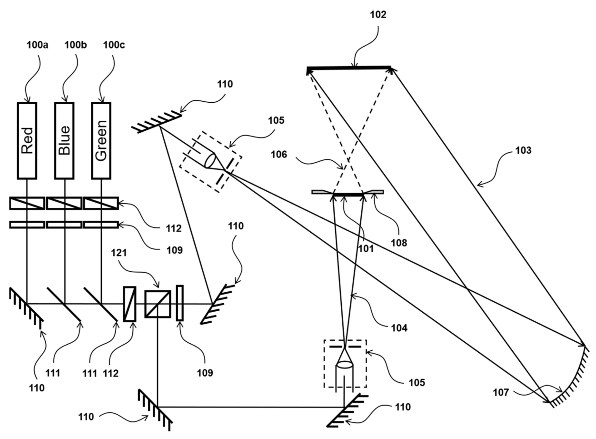
Figure 1 shows the scheme of the two-beam exposure setup of such a P-HOE as a transmission type HOE. An illuminated diffusor stripe forms the object beam and a plane wave forms the reference beam. The setup is able to expose RGB HOEs simultaneously. However, it could be also used for two wavelength spectral MUX or monochrome exposure by simply shutting off the respective lasers. A red laser is denoted by 100a, 100b denotes a blue laser, and 100c denotes a green laser as light sources. For the red laser a Krypton Ion laser (Coherent, Innova Sabre) with a specified output power of 2.1 Watt at λ = 0.647 µm was used. The green laser was a DPSS laser (Coherent Verdi V5) with a specified output power of 5 Watt at λ = 0.532 µm. Finally, the blue laser was an Argon Ion laser (Coherent, Innova 305) with a specified output power of 0.9 Watt at λ = 0.488 µm.
Furthermore, individual shutters 112 configured for blocking a laser beam were provided. In particular, each of these lasers can be blocked by individual shutters directly after the laser output. In addition, a main shutter exists. The main shutter was configured to control the simultaneous exposure time texp for up to all three laser wavelengths.
The beam ratios (BR) between the power density of the reference beam Pref and the object beam Pobj of each individual laser wavelength λ were adapted with the half wave plates 109 located after the individual shutters and the polarizing beam splitter 121. Thereby, BR is defined as follows:
Pref and Pobj were measured with photodiode sensors at the location of the recording element 102 with the sensor planes aligned parallel to the HOE plane. In the present example, the polarizations of all recording beams were set to S-polarization with respect to the plane of the recording table. The three laser beams were coaligned by the aid of one mirror 110 and two dichroic mirrors 111. The reference beam 103 was expanded by a spatial filter 105 and directed on a spherical mirror 107 with a focal length of 3000 mm. The pin hole of the spatial filter 105 was placed into the focal point of the spherical mirror to generate the collimated reference beam. The reference beam was directed at an incidence angle of 30° in the air towards the normal surface of the recording plate. The object beam 106 was generated by the diffusor 101 and apertured by frame 108, which was illuminated by a divergent beam 104, generated by another spatial filter. The main optical axis of the object beam was centered and oriented perpendicular towards the recoding element. The P-HOE itself was apertured to a height of 532 mm and a width of 312 mm and the diffusing object was apertured to a height of 65 mm and width of 500 mm. The distance between the diffusing object and the recording element was set to 1000 mm. The total power densities Pref + Pobj of ~100–200 µW/cm2 can be reached at an output power of the green laser in the range of 1 W to 2 W. To minimize the recording of intermodulation noise generated by the diffusing object the BR was set typically to ~13.
2.2. Beam (B)-HOE Recording and Recording Setup
The B-HOE serves to illuminate the full size of the P-HOE, if locally illuminated by a pencil of light which is a part of the plane reference beam used to expose the B-HOE. B-HOE and P-HOE have to be positioned to each other in such a way that the illumination direction of the P-HOE generated by the diffracted light of the B-HOE should be the direction—with respect to the polar angle of incidence of the reference beam—used to record the P-HOE. From this, the illumination point on the B-HOE together with the optional further collimating of films or sheets serves as an object point for the P-HOE. The view box generated with high efficiency by the P-HOE can be steered in one parallax depending on which local position the B-HOE is illuminated by the pencil of light under the proper angle.
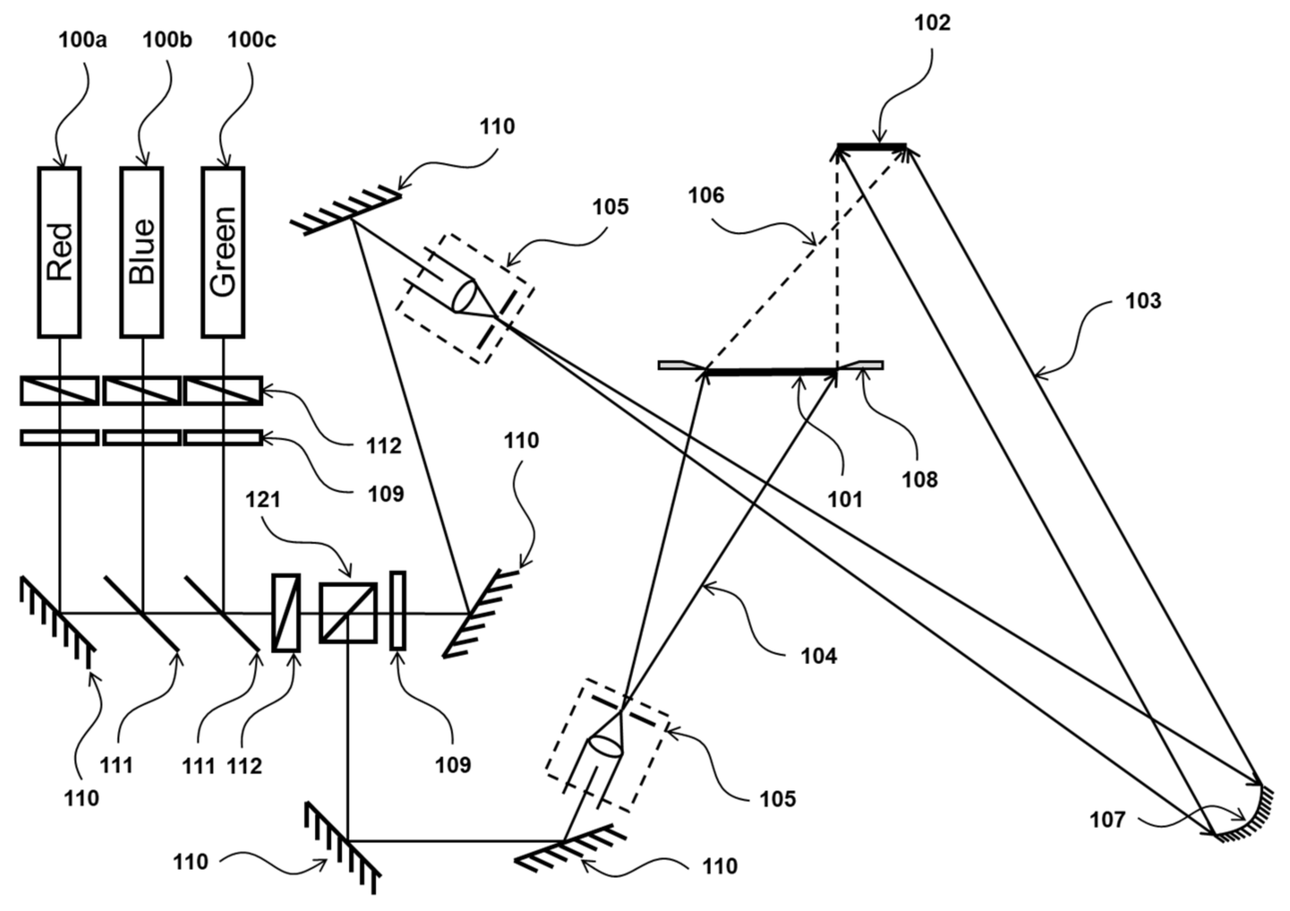
Figure 2 shows the scheme of the two-beam exposure setup of the B-HOE, a transmission type HOE from a rectangular shaped diffusor forming the object beam but offset with its center to the center of the recording element and a plane wave forming the reference beam.
The used components and their labelling were the same as used for the P-HOE recording as the incident angle of the reference beam was unchanged. However, the incident angle of the main optical axis of the object beam changed from 0° to −26°. Moreover, some dimensions changed. The recording element 102 of the B-HOE was apertured to a 560 mm height and a 100 mm width and the diffusing object 101 was apertured to a height of 560 mm and width of 346 mm. The distance between the diffusing object and the recording element was set to 700 mm. Moreover, the B-HOE and the diffusing object were decentered horizontally by 213 mm to generate the −26° incident angle of the object beam. The total power densities Pref + Pobj of ~85–150 µW/cm2 can be obtained at an output power of the green laser in the range of 1–1.5 W with BR set to ~10–14.
2.3. BS-HOE Recording and Recording Setup
The purpose of the BS-HOE was to reconstruct the real image of a rectangular diffusor if illuminated by a point source of high NA in a reflection hologram configuration. In combination with the P-HOE, the BS-HOE served the same steering function as the B-HOE. However, the optical path was folded, reducing the total depth. Moreover, the steering can be facilitated by a single pencil of light being deflected for example by a 1-axis rotating mirror at the position of the point source of the reference beam used to record the BS-HOE.
Given the geometrical size of the BS-HOE, the size and distance of the real image of the diffusor and as well the high NA and distance of the point source to the recording element of 600 mm, it was impossible to record this BS-HOE directly. To generate a respective (phase-conjugated) converging spherical beam, the sheer size of the available optical components, mainly the converging mirrors with the respective high NA of at least 0.42 was highly limited. In addition, the available output power of a single frequency laser is far too low to expose a photopolymer. We therefore used a copy scheme at a close distance between the master HOE and the copy element. The formerly recorded B-HOE (either green only or red and blue simultaneously) was reconstructed with its phase conjugated plane reference beam (in fact we used the original reference beam and flipped the B-HOE) to form the real image of the diffusor and the diverging spherical reference wave was generated with a high NA objective (ZEISS LD Plan-NEOFLUAR 63 x/NA = 0.75 Korr.). We accept that we may have recorded in addition a ghost HOE between the zero-order beam of the B-HOE and the spherical wave. However, this ghost HOE did not hurt the final application in this case.
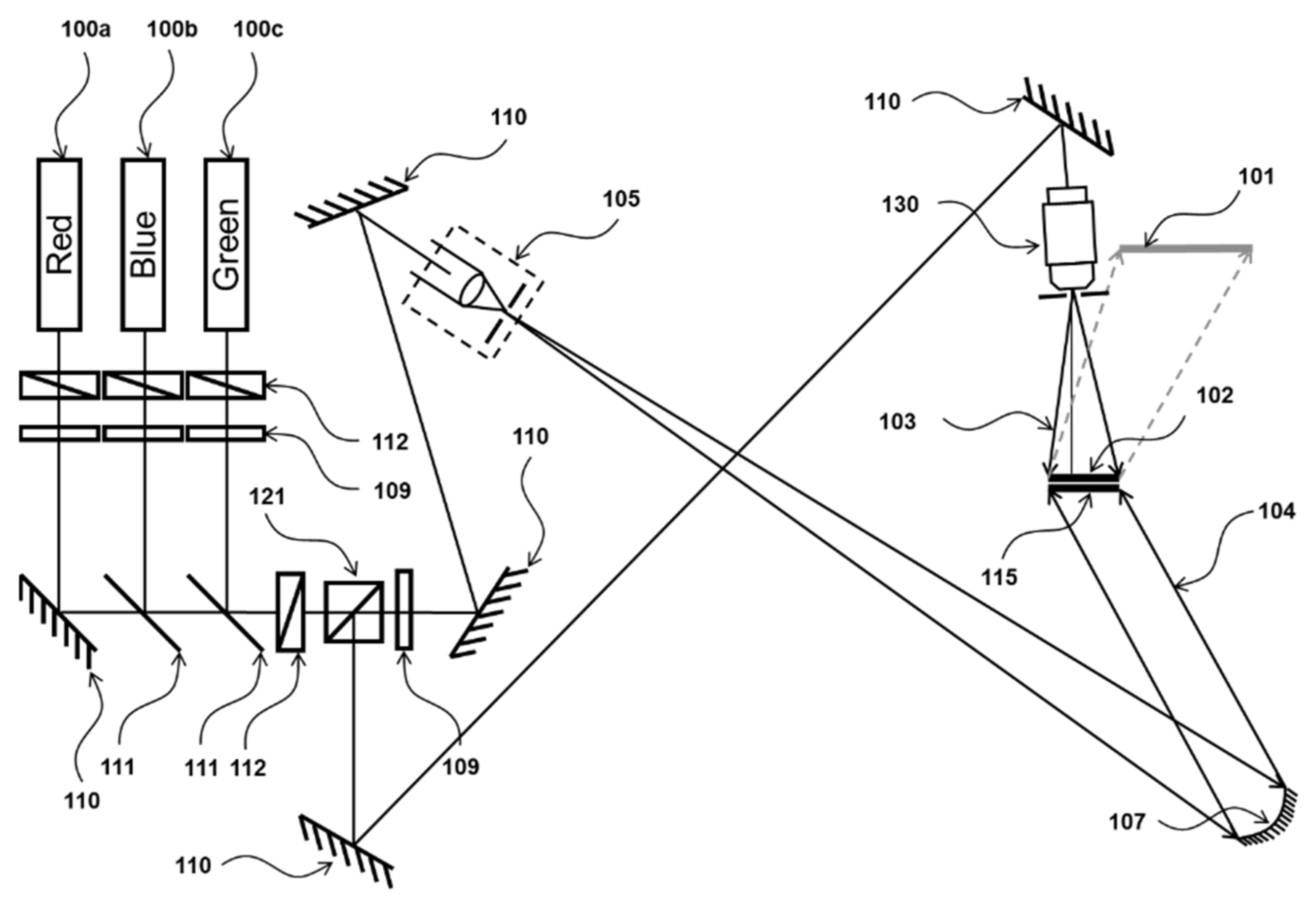
Figure 3 shows the scheme of the two-beam close distance copy exposure setup of the BS-HOE (stripe-like in shape) but offset with its center to the center of a high NA spherical wave forming the reference beam so that the optical axis with respect to the center of the copy element generated an incident angle of 8° in air.
In Figure 3, 115 denotes the flipped B-HOE now serving as a master HOE and 102 denotes the copy element instead of the recording element. The high NA objective is labeled 130 generating the new spherical reference beam 103. The grey part indicates the real image of the diffusor 101 emerging from the phase-conjugated replay of the B-HOE illuminated by the plane wave 104. All other components and their labelling are the same as for the P-HOE. The exit angle of the main optical axis of the real image was consequently −26°. The BS-HOE was recorded as either green only or red and blue simultaneously. In the first case the total power density Pref + Pobj of ~90 µW/cm2 can be reached at an output power of the green laser in the range of 1 W with BR set to ~2.5. In the second case the total power density Pref + Pobj of ~25 µW/cm2 can be reached at an output power of the red laser in the range of 0.77 W with BR set to ~4.3 Pref + Pobj of ~30 µW/cm2 for the blue laser at an output power in the range of 0.95 W with BR set to ~2.3.
As all setups were rather large and optical arm lengths were a few meters long, a fringe locker system was used to stabilize the setup for exposure times well above 600 s if needed. The recorded HOEs were bleached twelve hours on a light box to remove residual coloration from the photo-initiator system. To investigate the performance of the different types of the recorded HOEs with respect to the thermal fringe formation they were observed through the real images of the diffusors (the view boxes). In the case of the transmission-type HOEs, a strong white light source at a large distance (~5 m) was used. In the case of the reflection-type HOE, the spherical reference beam in the exposure setup was used.
3. Preliminary Experimental Analysis and Conclusions
In this section we describe the experimental evidence when thermal fringe formation occurs and when it does not occur. Thus, the problem can be further specified so that a physical model can be developed to describe the phenomenon quantitatively.
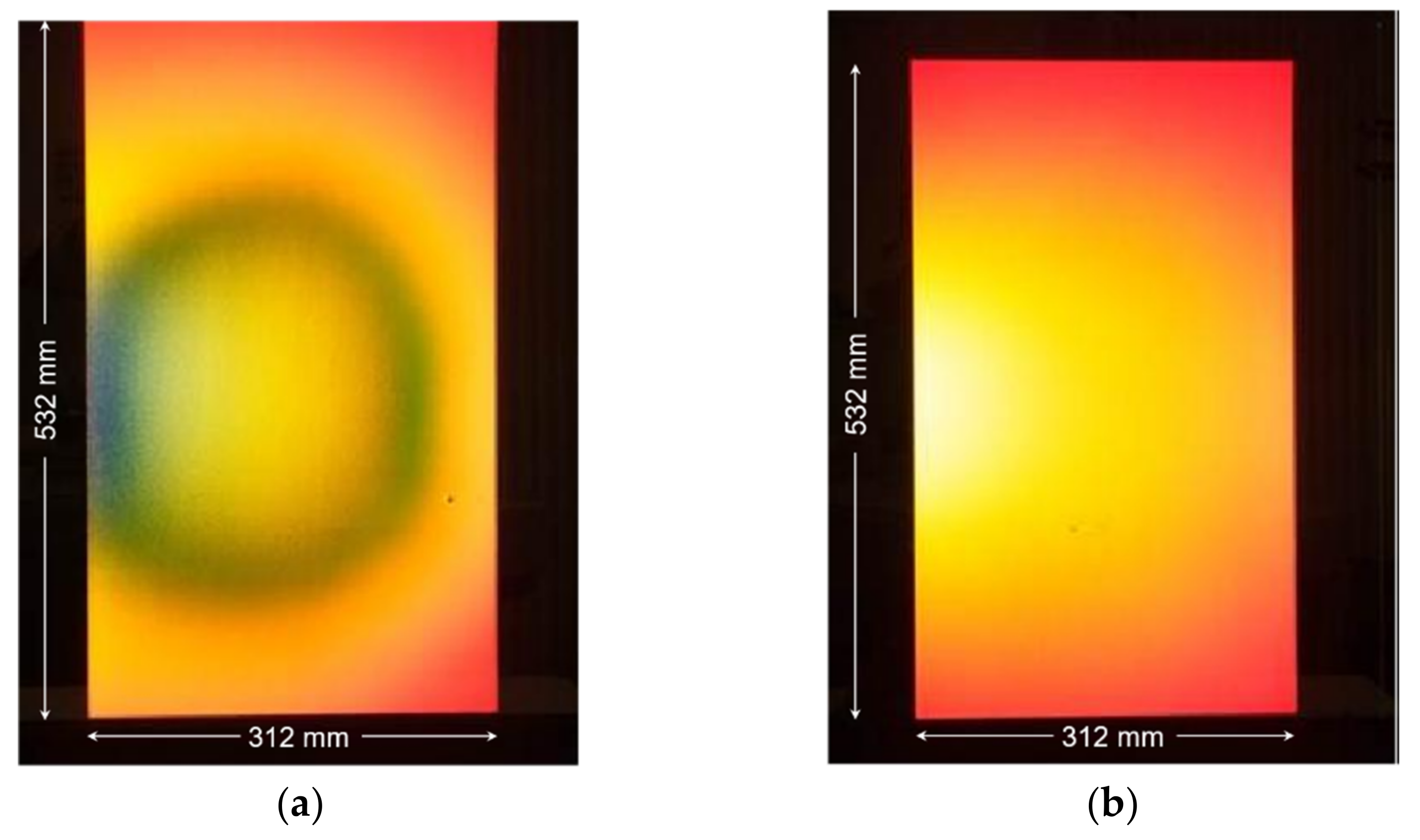
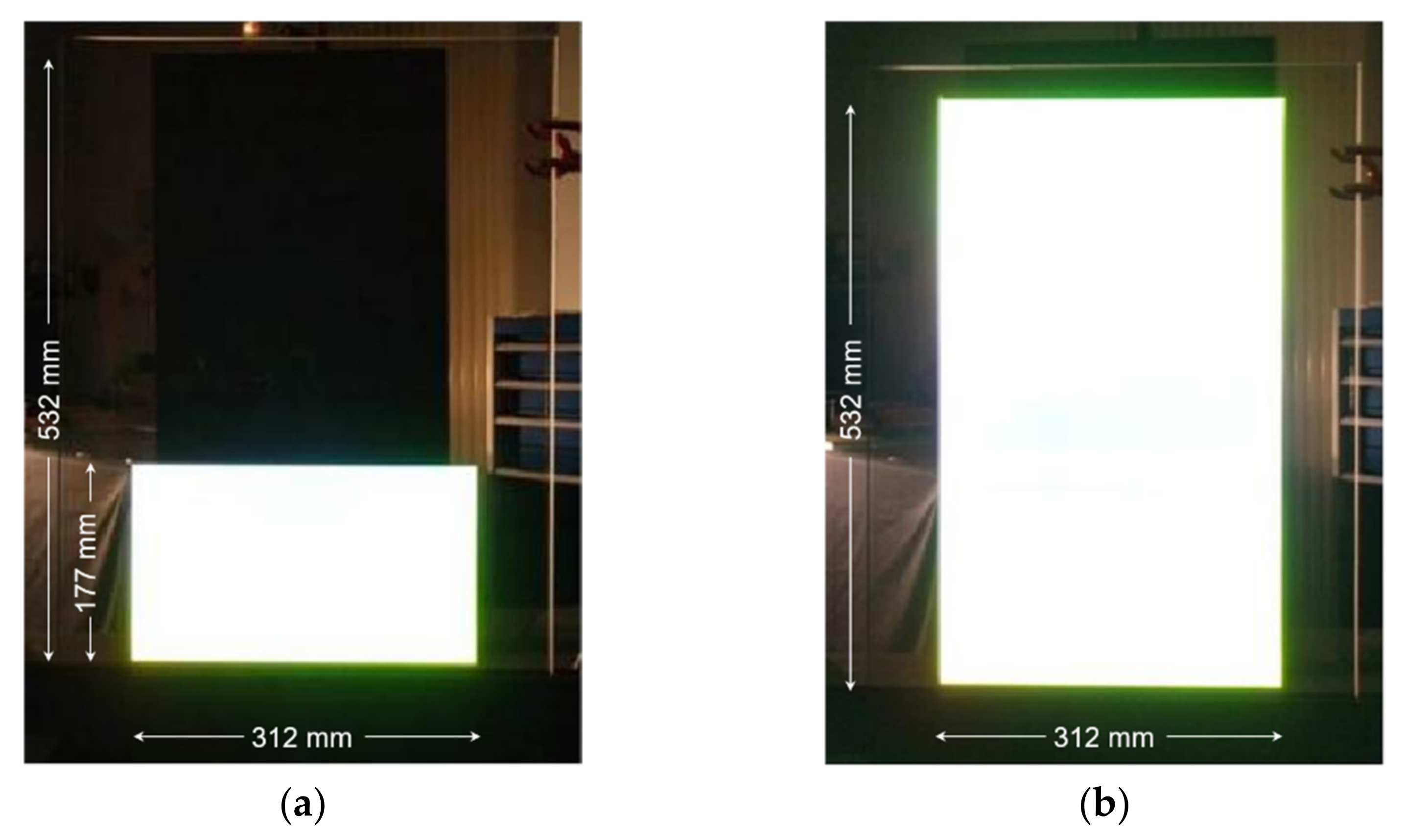
In Figure 4, examples are shown in which a thermal fringe appears or does not appear in a P-HOE. The pictures show the view into the P-HOE through the view box generated by phase conjugated reconstruction. Figure 4a shows a P-HOE in which the photopolymer was laminated on top of a 10 mm thick glass plate. Clearly a dark thermal fringe can be seen. Figure 4b shows the result of a repeated recording. However, in this case the photopolymer was sandwiched between two 10 mm thick glass plates, and clearly no fringe was observed. This suggests that if the recording happens in the mechanically “neutral” plane of a sandwiched recording element, no thermal fringe formation appears.
We have to note that the obvious solution of sandwiching the photopolymer film between glass plates is not a practical one. The sufficient mechanical contact is only given by chance and there is a high likelihood of generating defects in the HOE if the mechanical contact is given only locally (pressure marks).
The above observations imply that the fringe formation must have been caused by a movement and/or a bending of the recording element during the HOE recording. If the object (the diffusor) or the reference beam moved or changed their shape or wavefront, fringes should have appeared in the reconstructed real image or should be visible in the real time interferometric setup, which was not the case. The latter means that the virtual image or the reference beam can be observed by looking through the HOE and both—reference and object—beams are on. To further rationalize this phenomenon more experimental observations are listed below:
- Ratio of the glass plate lateral dimensions W or H over the glass plate thickness h.In the experiment described in Figure 4, the ratio of W/h is about 45 and the ratio of H/h was about 60. On average it was about 52.5. In earlier experiments in which we recorded a scaled HOE (66 mm by 110 mm) using a 3 mm thick glass plate of size of W = 90 mm by H = 120 mm, the respective average ratio was 35.0. In that case we never obtained a fringe during the P-HOE recording. On the contrary, when we replaced the large size recording experiment with the asymmetric recording element and the 10 mm thick glass plate with a 3 mm thick glass plate, we obtained two dark fringes within the recorded HOE area. Note that in this case the respective average ratio of lateral plate dimensions over plate thickness increased by up to 157.5.
- Fill factor of the recording plate.In the experiments above only part of the glass plate area was illuminated to record the HOE. We defined the fill factor as the ratio of the P-HOE area over the glass plate area (always smaller or equal to 1). In the large size HOE recording, the fill factor was ~0.647 and for the small size HOE recording it was ~0.672 and therefore was very similar to the fill factor in the large size HOE recording. We repeated the large size P-HOE recording using a 10 mm thick glass plate with a decentered exposure mask of 312 mm width and 177 mm height (only lower third of the original mask of 312 mm by 532 mm size). This means the fill factor was ~0.217. We further repeated this decentered recording with a reduced fill factor in sequence for the lower and for the upper third of the P-HOE in a first and in a second recording and in a third recording we exposed the full format. In both cases no fringe formation was observed (see Figure 5).
Figure 5.
The view into the partially (a) and consecutive (b) recorded P-HOEs from the position of the focal position of the real image of the diffusor (phase conjugated reconstruction). The fill factor was ∼0.217 for the partial exposures.
Figure 5.
The view into the partially (a) and consecutive (b) recorded P-HOEs from the position of the focal position of the real image of the diffusor (phase conjugated reconstruction). The fill factor was ∼0.217 for the partial exposures.

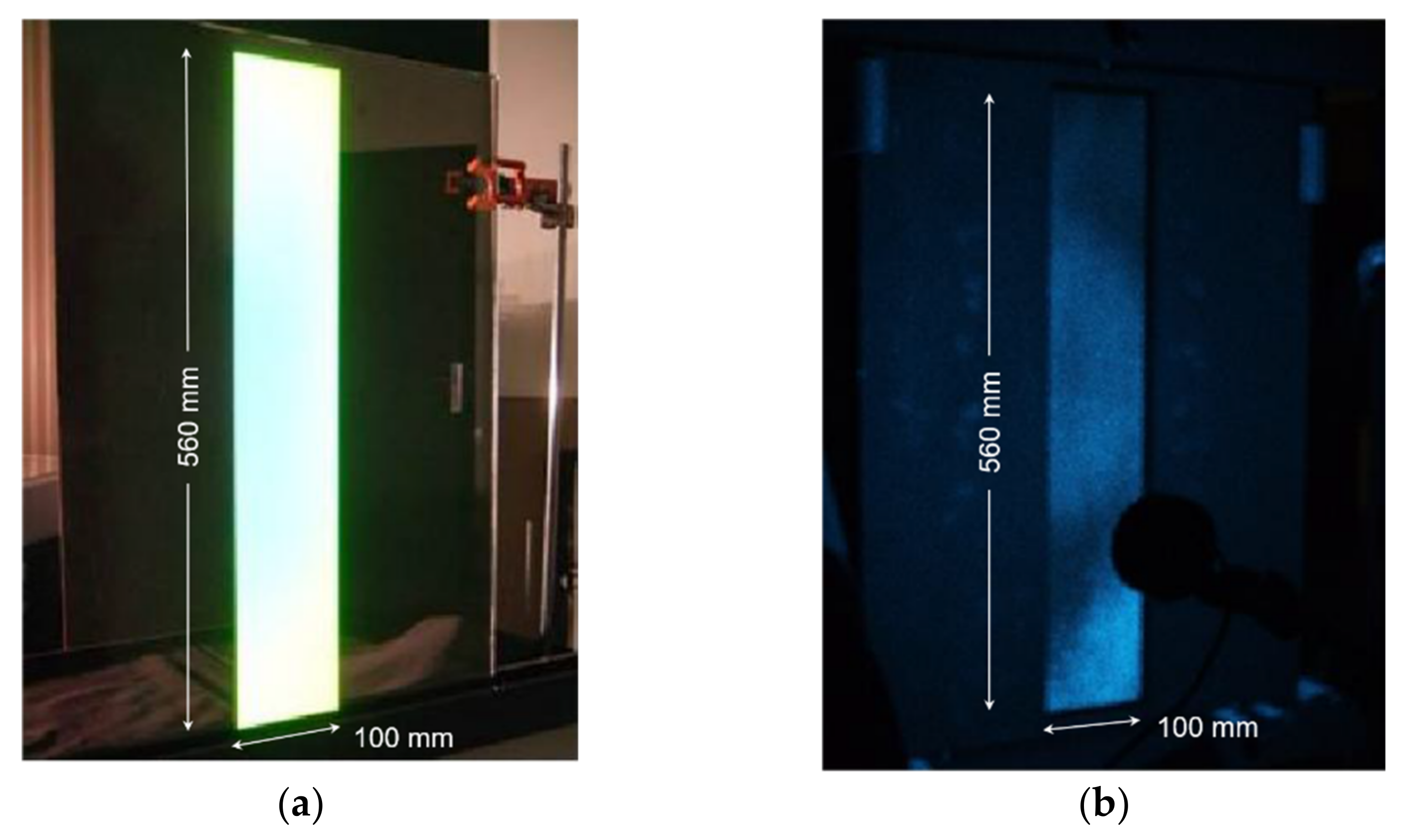
- Slant angle α (angle inside the photopolymer between the grating vector and the plate surface) of the recorded grating.The B-HOE, an almost non-slanted transmission hologram of a diffusor with α = 1.2°, was observed from the focal position of the real image of the diffusor (phase conjugated reconstruction) and showed no fringe. The same glass plate as above was used for the recording element but with a thickness h of 3 mm only. No fringe was observed (see Figure 6a). The BS-HOE was a reflection hologram generated by a two-beam copy process using the B-HOE as a master hologram. In this case the slant angle α was about 84°. The thickness of the glass plate h was 10 mm. This reflection hologram showed strong fringe formation (see Figure 6b).
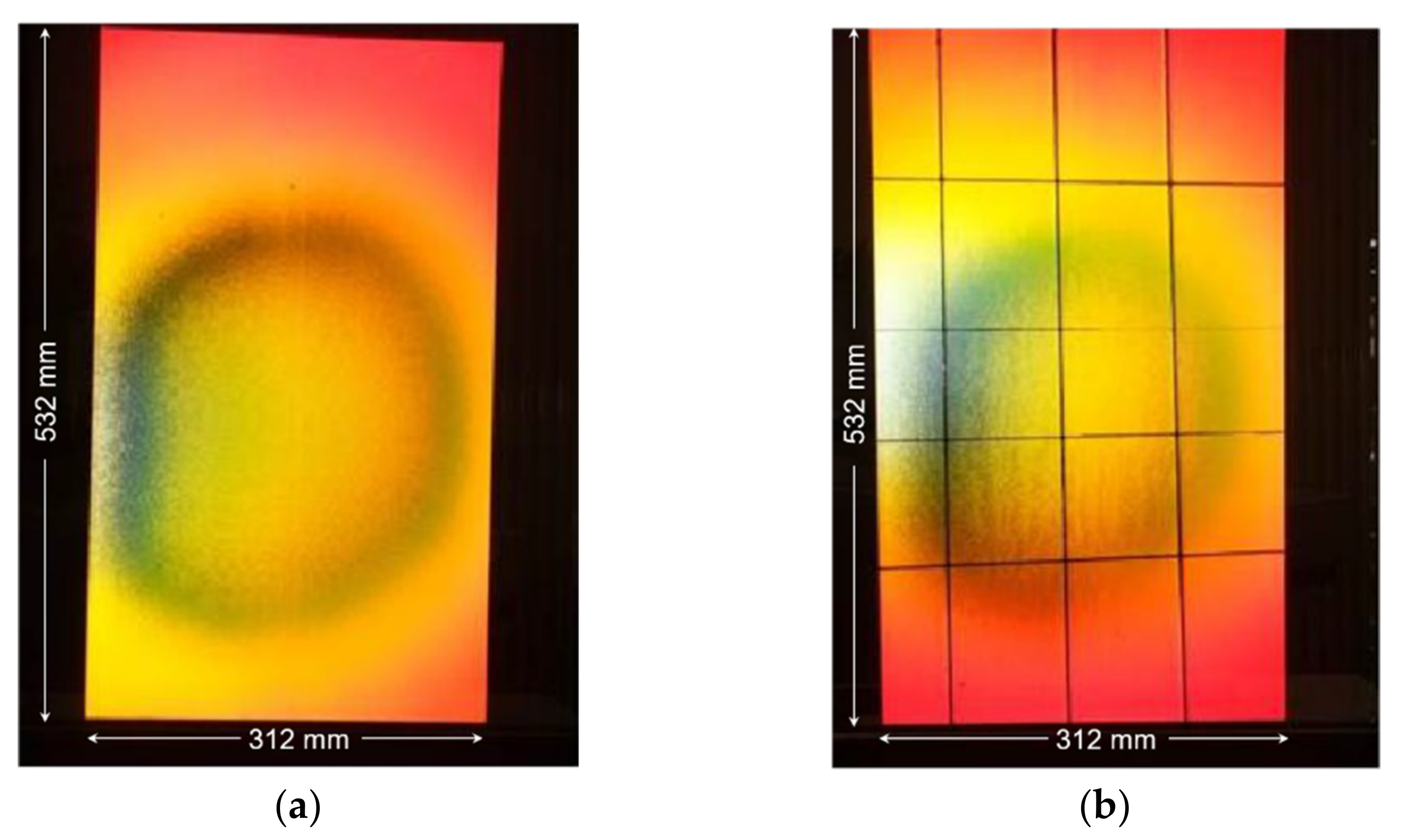
- Shrinkage s of the photopolymer during the exposure interval.Shrinkage is caused due to the volume reduction by photopolymerization in acrylate-based photopolymers. In the recording stack setup, the photopolymer was adhered to the glass and the substrate, the volume shrinkage was completely transferred by a thickness shrinkage s. However, at the edges of the HOE area the translational symmetry along the plate surface was broken and shear stresses might have occurred which give raise to torques that finally could bend the full recording element. To investigate this in more detail we again used the large size P-HOE recording experiment. However, in this case we crosscut the laminated photopolymer layer through the substrate down to the glass into small rectangles (similar size of the small size P-HOE recording) before exposure. Still the fringe formation occurred (see Figure 7).
Figure 6.
(a) The view into the B-HOE from the position of the focal position of the real image of the diffusor (phase-conjugated reconstruction). (b) The view into the BS-HOE, a two beam reflection copy of the B-HOE. Recording was performed with 0.647 µm and 0.488 µm simultaneously and the reconstruction was performed with 0.488 µm only.

Figure 7.
View into the P-HOE from the position of the focal position of the real image of the diffusor (phase-conjugated reconstruction). (a) A P-HOE in which the photopolymer was laminated on top of a 10 mm thick glass plate. (b) The result of a repeated recording. In this case the photopolymer was crosscut into small rectangles before recording and was still laminated onto the glass substrate.

From the above experimental results, we can conclude the following: First, we can exclude shrinkage as a primary source of this fringe formation because if shrinkage was decisive, the crosscut photopolymer layer would not show fringe formation. The exclusion of shrinkage would be also physically reasonable, as in the case of Bayfol® HX film the photopolymer is a soft rubber with a relatively low storage modulus but a non-zero loss modulus, and therefore has the ability to creep. This material might not be able to exert a large enough torque to bend the recording element.
Second, as shrinkage is excluded the only possibility to bend the recording plate is by asymmetric heating. This means that by the interaction with the recording light one surface of the recording element has a different temperature than the second surface during the exposure period. By thermal expansion, this temperature difference over the thickness of the glass plate can lead to a bending of the recording element.
Third, asymmetric heating during the HOE recording can only happen either by conversion of the absorbed light into heat and/or by the heat of polymerization, always during the exposure interval of duration texp.
Fourth, the fringe formation can be influenced by the ratio of the lateral plate dimension H or W over the plate thickness h and the fill factor of the HOE area versus the plate area .
Fifth, the fringe formation at a given fill factor and a given ratio of the lateral plate dimension over the plate thickness depends heavily on the slant angle α and the grating spacing or equivalent to all of this if we record a transmission or a reflection hologram. Obviously, fringe formation is more severe for reflection holograms which have subwavelength grating spacings and grating layers that are more or less perpendicular to the potential movement direction of the deforming recording element.
Therefore, the bending of the recording element by a heating of the photopolymer layer has to be understood through an appropriate quantitative physical model. If this is achieved, all parameters involved will be immediately identified and measures against this fringe formation can be found and implemented very easily.
4. Bending Deformation of a Thin Disc by Thermal Imbalance
In this section we derive the bending behavior of a thin, elastic disk under the constraint that on one surface heat is generated by the interaction of a photopolymer layer with the recording light.
To describe our holographic recording situation in which a rectangular plate was used and at the same time to simplify the mathematics, we made the assumption that our plate had a circular shape of effective radius R and a thickness h. The ratio R/h was simply approximated by the largest value of the ratios and . Moreover, should be much larger than 1 (which is usually the case for our large size HOE recording), so that our plate or disc could be considered to be a thin, elastic plate or disc. Let us describe the disc bending deformation by the deviation ξ(r; t) of the z-coordinate from 0, in dependence of the radial position r and the time t as a parameter. To find the solution for ξ(r; t), first the free energy F of such a deformed disc has to be minimized with respect to ξ(r; t), including the contribution of the heating on one surface. This will give us the equation of motion for ξ(r; t), namely . This equation of motion can then be solved using the appropriate boundary conditions. Note, that the contribution of heating on one side of the disc to its free energy F enters into F via the boundary conditions at r = R. How to solve this variation problem, with the help of [12], is described in [13].
We will treat two specific cases for the boundary conditions.
- A clamped disc case:
- and a supported disc case:where σ is the Poisson ratio of the disc material. There were two additional boundary conditions which are not listed here, as they were identical for both cases. One contains the Young’s modulus materials EY and the Poisson ratio materials σ and the heating term on one surface. The heating should occur at the surface located at z = 0, whereas the second surface is located at z = h. None of the two specific cases describes our recording situation completely, as the recording element is usually fixed to the holder by three pins, which would be very complicated to handle analytically. However, they should be good enough to obtain an estimation of the deformation, as we can expect that any real fixation should fall somehow in between these two cases.
4.1. Theoretical Treatment of the Deformation on a Clamped Disc Case
If we introduce the scaled radius coordinate = r/R the solution for the bending deformation ξ can be expressed as:
The term includes all material parameters and the influence of the heating on the one surface. It can be expressed as follows:
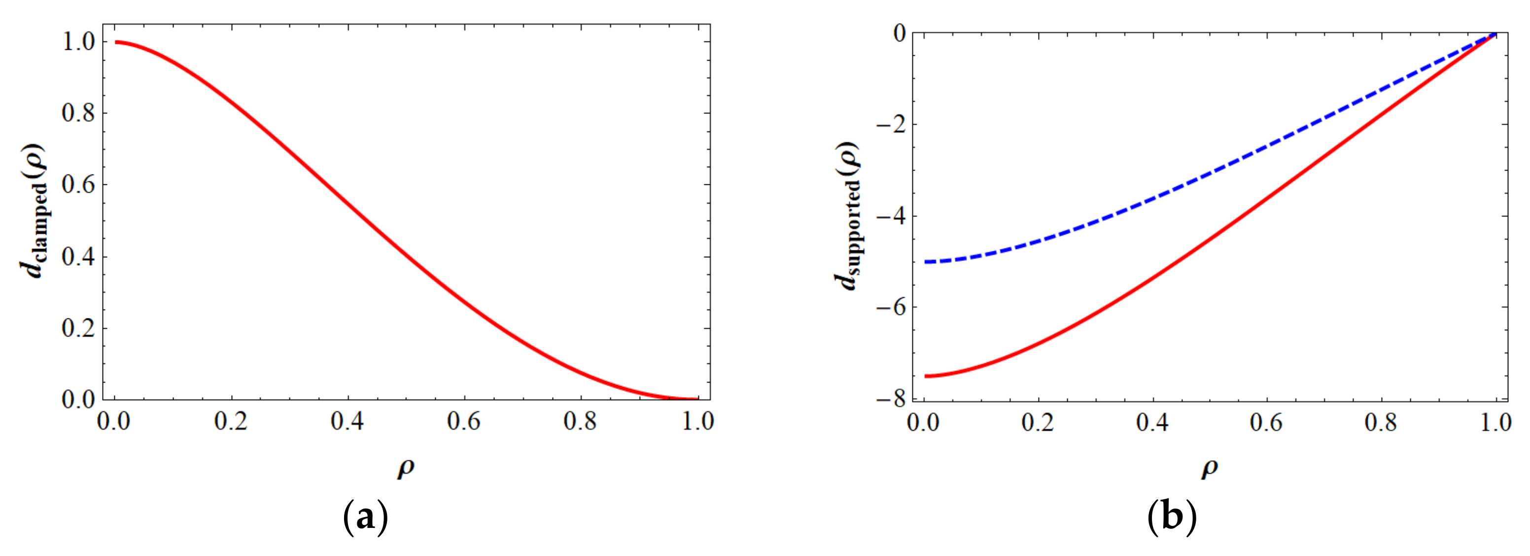
CTE is the coefficient of linear thermal expansion of the disc material and ζ is the normalized thickness coordinate , which is centered on the neutral plane of the disc. T(z; t) is the solution of the thermal diffusion equation between and , with the one-sided heating at the surface at . Finally, is the thermal imbalance caused by the heating from only one surface. The normalized bending deformation function of the clamped disc dclamped is given below as Equation (7) and as a plot in Figure 8a.
As expected in the center of the disc we will have the largest deformation.
4.2. Theoretical Treatment of the Deformation on a Supported Disc Case
In the case of a supported disc the deformation can be expressed as:
The normalized bending deformation function of the supported disc dsupported is given below as Equation (9) and as a plot in Figure 8b.
As expected, again in the center of the disc we will have the largest deformation. However, the polarity was different compared to the case of the clamped disc. Note that a smaller Poisson ratio σ is in favor of a smaller absolute deformation. The supported disc will be always worse in terms of the absolute deformation compared to the clamped disc, even at the unrealistic value of σ = 0.
This analysis shows that at a fixed thermal imbalance the bending deformation ξ would scale as . This implies that for a large HOE recording in which R has to be increased for example linearly, the plate or disc thickness h would have to be increased quadratically to keep the deformation on the same level. This would lead to the necessity of using very thick glass plates to avoid fringe formation. The weight of such thick glass plates would become impractical for manual handling. For example, a 600 mm by 450 mm by 10 mm glass plate already has a mass of almost 7 kg.
As the thermal imbalance is caused by heating on one of the disc surfaces and this heat is dissipated mainly by thermal diffusion, the transient temperature behavior could also depend significantly on the thickness h. This could change the scaling behavior of ξ by drastically. Therefore, the term γ(t) has to be investigated more in detail. This will be carried out in the next section by solving the thermal diffusion equation for the appropriate boundary conditions.
5. Temperature Profile Evolution across the Thickness of the Recording Element
In this section we evaluate the transient behavior of the temperature profile across the thickness h of the disc if heating occurs just at one surface. This heating term A shall occur at the surface located at z = 0 and can be written as:
In Equation (10), ES describes the absorbed or generated energy per volume within a thin layer of thickness d. As the photopolymer layer is the active layer, d can be identified as the photopolymer layer thickness. It was also assumed that this energy is deposited homogenously within the exposure interval of length texp. In reality, this process will be much more non-linear [14]. However, within the framework of this study we will stick to this linear heat generation process with time. cP is the heat capacity per volume at constant pressure of the disc material. To have a more useful measure of the amount of heat generated, one can replace by ΔTad which is then the adiabatic temperature increase caused by ES within the photopolymer layer of thickness d. As the photopolymer layer and the substrate are very thin compared to the disc, heat conduction will be very quick (for a typical photopolymer layer the thermal diffusion time is ~0.2 ms and for a typical substrate it is ~2 ms). So, the photopolymer and substrate could be treated as one layer (with a larger thickness but also a larger heat capacity). For the other surface at z = h we can have two different boundary conditions. Either this surface is thermally isolated or it is maintained at a fixed temperature say 0 °C for convenience. Therefore, we have:
- a thermally isolated surface case:
- an isothermal surface case:
5.1. Theoretical Treatment of a Thermally Isolated Surface Case
The disk is heated on one side by either the heat of polymerization and/or the absorbed recording light. The other side should be thermally isolated. We then can write (see [15]):
D is the thermal diffusion coefficient which is related to the thermal conductivity ΛT and the heat capacity cP via . By a separation of the variables and Fourier expansion the solution of Equation (13) can be found easily (see Appendix A).
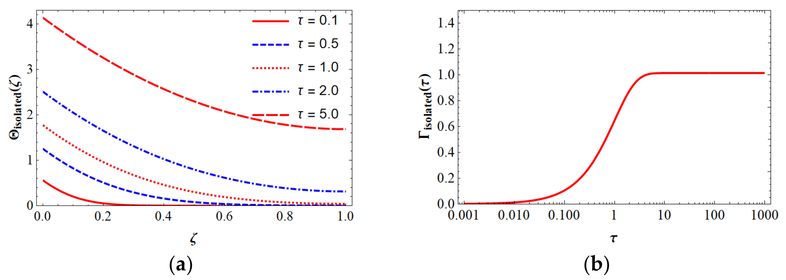
whereas is the dimensionless thickness coordinate and is the dimensionless time in units of the thermal diffusion (or relaxation) time . Some examples of Θisolated(; τ) are depicted in Figure 9a. At τ ~1 the temperature profile reaches the non-heated surface. At τ > 2 the curve simply moves up linearly in time without further changing its shape and curvature. To calculate the solution in Equation (14) has to be taken at T( + ½; τ). The result of the total integration is:
5.2. Theoretical Treatment of an Isothermal Surface Case
The solution can be found by the same procedure as in the thermally isolated case and is depicted in Appendix B. In the dimensionless and scaled spatial and temporal coordinates ζ and τ we find:
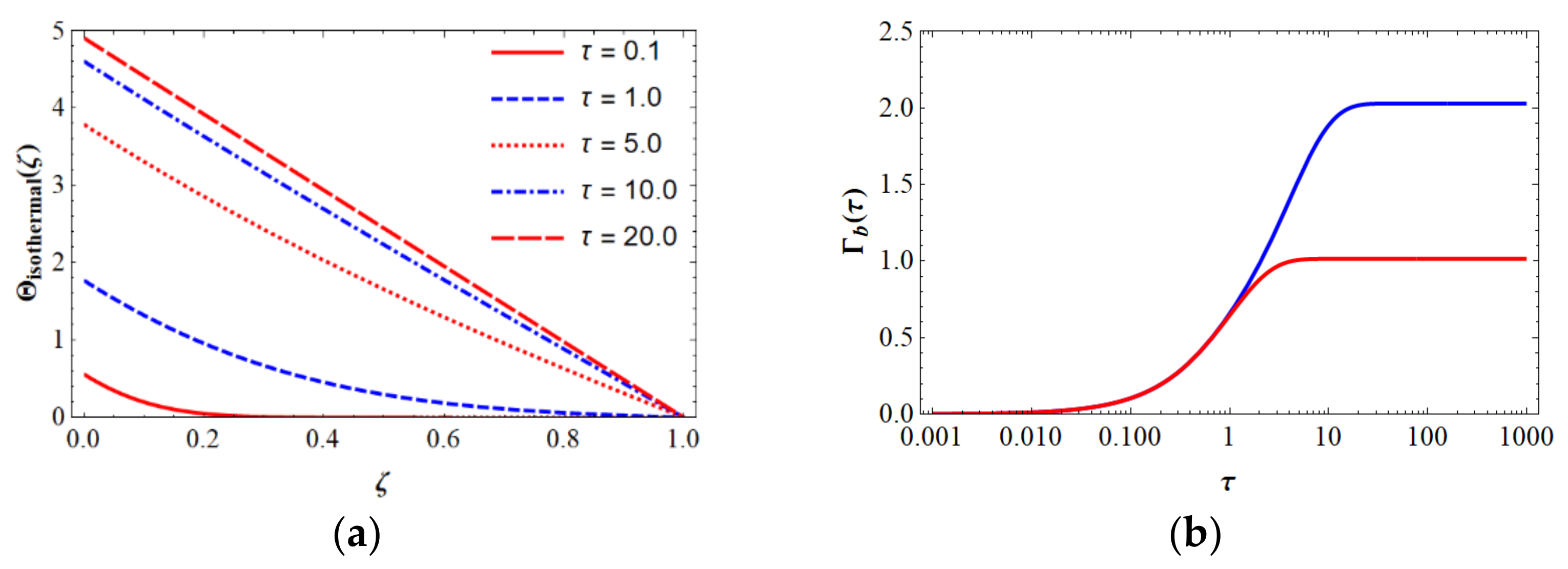
Some examples of Θisothermal(ζ; τ) are depicted in Figure 10a. Again, at τ ~ 1 the temperature profile reaches the non-heated surface. At τ > 10 the curve simply does not change further and there is a constant flux of heat from z = 0 to z = h. The thermal imbalance for this case is given as:
In Figure 10b the shape of Γisothermal(τ) is displayed versus the normalized time τ (blue line). Moreover, from Figure 10b it is obvious that there is no difference in the universal thermal imbalance term Γ—either isolated or isothermal—given in the scaled time τ as long as we have τ < 1. This is clear, as in the isolated case and in the isothermal case as well for scaled times τ < 1 the temperature profile does not see the non-heated surface at z = h and therefore behaves as it would develop in a semi-infinite media. However, beyond τ = 1 the universal thermal imbalance term Γ in the isothermal case can achieve twice the value as that of the isolated case. This is immediately clear if we look at the transient development of the temperature profiles given in Figure 9a and Figure 10a. So, that means it is preferential to have the non-heated surface isolated instead of thermalized to a fixed temperature, e.g., by cooling plates, bad heat transfer to air, etc.
In general, we end up with the expression for the local, transient bending deformation of a one-sided heated disc with:
where a can be identified with clamped or supported and b can be identified with isolated or isothermal. Equation (18) gives some immediate insights. The spatial and transient shape of ξa,b shows universal behavior and depends on the scaled coordinates in space and τ in time. Both scaled coordinates are separated in individual functions. There are three factors that serve as amplitude factors determining the absolute bending deformation if the scaled coordinates in space and time are fixed.
- The first amplitude factor describes the influence of the active recording layer when it interacts with the recording light within the exposure period . That means that at a fixed exposure dosage E (which will be determine the level of ) the deformation will be lower if the dosage is reached at a longer exposure time; this will be similar if the recording is performed at a lower power density P. If τ0 is small this will reduce the deformation further. Therefore, glass with a high thermal diffusion coefficient D will be beneficial. To reduce the excitation , photopolymer formulations with low absorptions and a low heat of polymerization will show smaller bending deformations.
- The second amplitude factor describes the response of the glass disc on the temperature gradient over the disc thickness via the CTE. Therefore, glass with very low CTE can bring down the deformation to an uncritical level. It is important to recognize that this factor is totally decoupled from the disc geometry and the properties of the photopolymer formulation. Hence a low CTE glass will reduce the bending deformation in all circumstances.
- The third factor describes the ratio of the lateral dimension R to the thickness h of the disc. Now the scaling looks more relaxed because if we double R we should have to double h only to keep this ratio fixed. However, note that h enters into the scaled time via τ0. Therefore, the scaling of the bending deformation ξ with the ratio could be far from a quadratic function under certain circumstances.
As we have seen, Γ is a monotonically increasing function with τ. As for the fringe formation in holographic recordings, the local, maximum achievable bending deformation is decisive if we are interested in investigating ξ at the time of τexp.
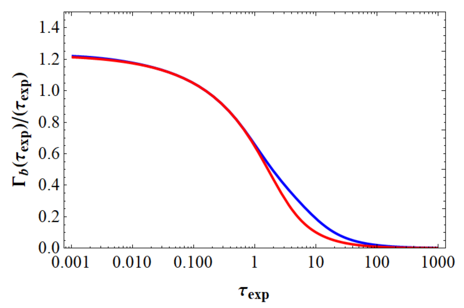
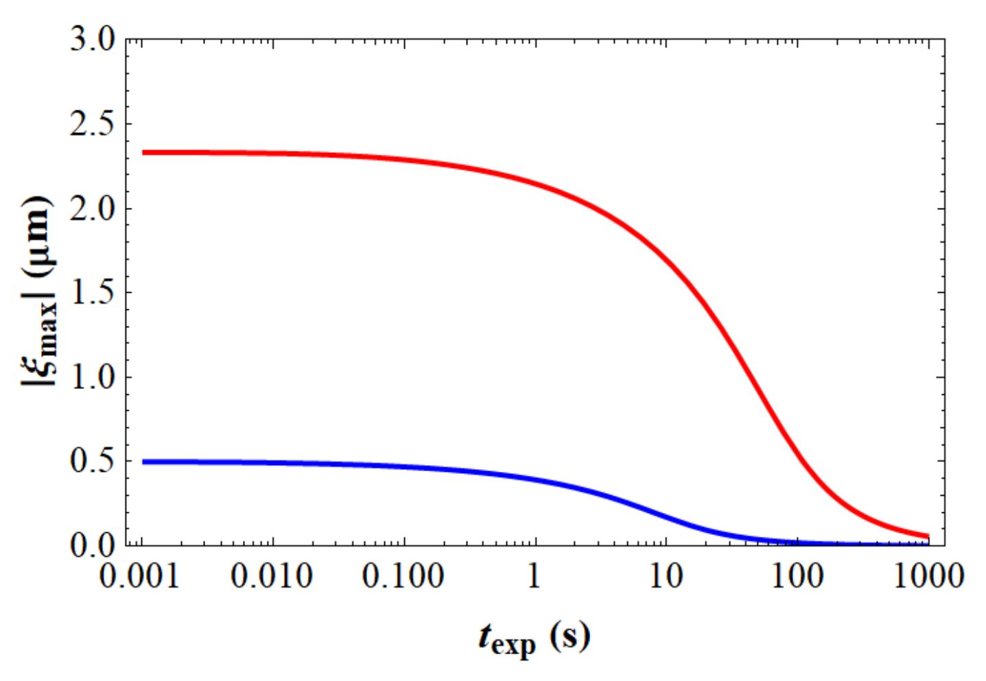
Equation (19) reveals that the term dictates the part of the local, maximum achievable bending deformation ξa,b that depends solely on the reduced exposure time τexp. is plotted versus τexp in Figure 11.
Figure 11 shows again that recording at a low power density for which the exposure time texp is much larger than the thermal diffusion time τ0 should effectively reduce the local, maximum bending deformation ξa,b. Moreover, here an isolated non-heated surface is preferred instead of a isothermal non-heated surface kept at a fixed temperature.
Equations (18) and (19) are the most general formulations of the heat-induced bending deformation within scaled variables in time and space and the separation in geometrical properties of the disc, the material properties of the photopolymer layer, and the material properties of the glass support. However, we have stated already that the thermal diffusion time τ0 still includes the disc thickness h and the thermal diffusion coefficient D of the glass support. Therefore, concrete estimations of the bending deformation ξ and the resulting fringe formation can be performed only after reviewing some material properties and recording parameters. This review will be completed in the next section.
6. Material Properties and Recording Parameters of Practical Relevance
In this section we list all relevant material properties and parameters of the recording and recording setup which are of importance.
6.1. Material Properties
In Table 1 a list of the material parameters of each layer of a recording element is given. The most important derived parameters are the thermal diffusion coefficient D and the thermal diffusion time of each layer τ0.
From Table 1 we can clearly see that τ0 within the photopolymer layer and the substrates are orders of magnitude smaller than those in the glass substrate. Therefore, thermal effects within the photopolymer layer and/or the substrate might only be important for CW holographic printers. For usual one-shot recordings in which for large size HOEs the exposure times are beyond 1 s, the photopolymer layer and/or the substrate can be thought of as behaving as a layer with zero thickness.
In Table 2, further material properties are listed. ∆HP is the exothermic heat of the polymerization of the photopolymer layer and Tini is its initial transmission at the recording wavelength λ. σ is the Poisson ratio and G denotes the elastic shear modulus.
6.2. Recording Parameters
For holographic recordings, the total energy dosage E which is necessary to record the sample to a satisfactory diffraction efficiency is usually decisive. This dosage E relates via the total power density P to the exposure time texp as follows:
E is given in mJ/cm2 and P is given in mW/cm2. For a photopolymer used in this study we take ~15 mJ/cm2 as a typical value for E.
6.3. Estimation of the Adiabatic Heating
As stated above, the only source for plate bending would be the heating of the photopolymer layer by the exothermic polymerization reaction and/or the absorption of the recording light. In the case of the exothermic heat of polymerization, the adiabatic temperature increase ∆Tad can be estimated by:
denotes the fraction to full conversion which can be achieved during the exposure interval. As a reasonable estimation we can set it to . In Equation (21) we can use ∆HP in J/cm3 and cP in J/(cm3·K) to obtain ∆Tad directly in K. In the case of the absorption of the recording light we first assume the worst case, that the sample does not bleach during texp. Then the absorption is fixed during the exposure to about (100%—Tini—Fresnel losses). Only this part of the total recording dosage E has to be considered as being responsible for heating. As the Fresnel losses are about 10%, the absorption is ∼50% if we take the value of Tini from Table 2. We can then write:
The factor 10 in Equation (22) enables us to obtain E in mJ/cm2, d in µm, and cP in J/(cm3 ·K) to obtain ∆Tad directly in K. Inserting the values listed in Table 1 and Table 2 into Equations (21) and (22) we immediately obtain:
- For the effect caused by the heat of polymerization:
- For the effect caused by the recording light absorption:
As we can see, the effect of the heat of polymerization is more than 13 times larger than that of the absorption of the recording light. Therefore, it would be more fruitful to avoid fringe formation by concentrating on photopolymer formulations with a low ∆HP or keeping f(texp) small, which means profiting from a long-lasting dark reaction to achieve a high efficiency.
7. Some Parameter Case Studies for the Bending Deformation
In this section we simulate the real maximum bending deformation ξmax of the disc for some typical recording conditions of large sized HOEs. As the source for heating, we will consider only the heat of polymerization represented by ∆Tad = 33.25 K. The photopolymer layer thickness d was fixed to 15 µm. We will focus on the clamped disc case and the isolated thermal boundary condition of the non-heated surface. In the clamped disc case, is the maximum value. In this case we can reveal Equation (19) as:
7.1. Variation of Disc Thickness h and Disc Radius R and CTE
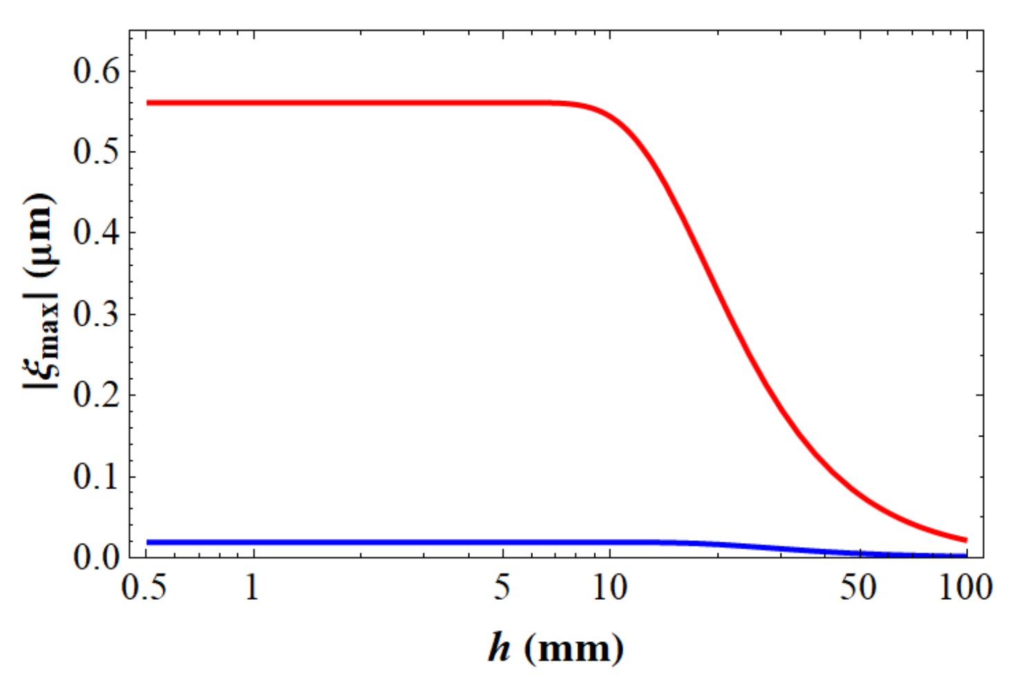
At first the dependency of ξmax on the disc thickness h was investigated for two different glass types of the recording element. We assumed that the recording dosage E was 15 mJ/cm2 and texp = 100 s which corresponds to a power density P = 150 µW/cm2. This is a typical value at the upper level that can be achieved if a large size P-HOE of dimensions depicted in Figure 4 is recorded with a laser with an output power of 1–2 Watts. If we take R as the maximum recording element extension, we end up with R = 600/2 mm. In Table 3 we list the guiding properties in dependence of the disc thickness h.
As can be seen for small h, the ξmax value does not depend at all on h, whereas after a certain cross over value of h, ξmax starts to decay with an increase in h. This crossover occurs around τexp~1 as expected. Therefore, increasing the plate thickness will not reduce plate bending in all cases but only if a critical value of h has been overcome. Below this critical value of h, the saturation level then depends solely on the CTE and the R2 if the exposure time texp is fixed! The influence of the CTE on the ξmax, its behavior with disc thickness h is compared between float glass and Nextrema® in Figure 12.
As an illustration of the influence of R on the ξmax, the behavior with a disc thickness h is given in Table 4 for the smaller sized P-HOEs for exactly the same other conditions as used in Table 3.
Clearly, we can see that for small format P-HOEs recording, the plate bending is reduced considerably. Even if we use very thin glass plates, their bending is so low at the exposure time of texp = 100 s that it will not cause any fringe formation. We have investigated in this section the influence of the geometry of the recording element, its CTE and the bending deformation ξmax. We will have a look at the influence of the recording time texp or the equivalent recording power density P in the following section.
7.2. Variation of Exposure Time texp or Recording Power Density P
For this case study we assumed again that the recording dosage E was fixed at 15 mJ/cm2. If we then vary texp this means that the recordings will be carried out at different power densities P. The disc thickness h was set to 10 mm for a float glass support and R = 600/2 mm was used for the large size P-HOE recording. We assumed limiting values for texp = 0.001 s and texp = 1000 s. The low value is characteristic for holographic printing, in which the high-power density is achieved by focusing down the laser beams to a small area. At the latest in this case the thin plate approximation may break down as the sub-hologram size R is comparable to a realistic HOE support thickness h. Further, this exposure time is already in the range of the thermal diffusion time in the substrate. So below this value we can no longer assume that the heating in the photopolymer film can be treated as if it would happen in a layer of zero thickness. The high value would translate into a power density of p = 15 µW/cm2. At this low power density level recording starts to fail because oxygen inhibition cannot be overcome. Note that the dissolved oxygen in the substrate will diffuse into the photopolymer layer at a comparable or higher rate as it is consumed by the initiation step. In this case the polymerization will not start anymore. In Table 5 the results of this investigation are listed. Again, at exposure times texp which are much lower than τ0, the disc bending ξmax is rather large and saturated. If texp is much larger than τ0, ξmax quickly decays with increasing exposure time. So, at a given geometry and material of the glass substrate, ξmax and therefore the risk for fringe formation can be reduced if the exposure time can be increased by recording at low power density P. The influence of the CTE on the ξmax and its behavior with the exposure time texp are compared between float glass and Nextrema® with their typical thicknesses in Figure 13.
Obviously, even when using a low CTE glass, ξmax can reach values of ~0.5 µm if the exposure time is short enough. It is also interesting to see the cross over shift to smaller exposure times in the case of Nextrema® because its thermal diffusion time is much smaller as for the float glass. The reason for this is that Nextrema® has more than twice the thermal diffusion coefficient and almost half the thickness of the float glass, which shortens τ0 by a factor of ~6 compared to float glass. Again, an illustration of the influence of R on ξmax and its behavior with exposure time texp is given in Table 6 for the smaller sized P-HOEs for the same conditions as used in Table 5.
This time we can also see that for a small format P-HOE recording, the plate bending ξmax can reach high values above 1 µm. Namely, the recording was completed at a power density which was too high which led to an exposure time texp that was too low.
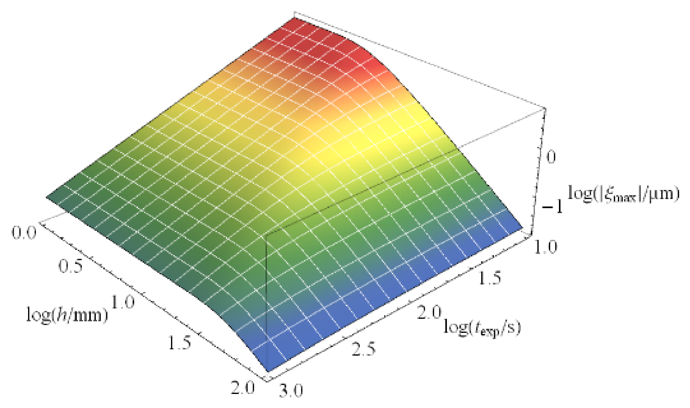
In the above case studies, we have seen that if fringe formation happens by plate or disk bending or not, the conditions could show quite complex behavior that is difficult to predict by looking at only one isolated parameter. For example, increasing only the thickness h at a fixed size R of the recording support could be totally inefficient to avoid the thermal fringe formation or changing the observed fringe pattern as it increases the thermal diffusion time τ0 in the glass substrate. As a consequence, ξmax may not change at all if texp is not already or cannot be brought in a favorable regime. Decreasing only the recording power density P or equivalently increasing the exposure time texp, keeping the exposure dosage E fixed, may also lead to a complete insensitivity of ξmax, if the thickness h of the recording support is too large. Lowering the CTE and increasing the thermal diffusion coefficient D of the glass substrate helps in any case to reduce ξmax. In Figure 14, ξmax is plotted versus h and texp in the case of the use of a float glass plate as a recording support with an equivalent radius of R = 300 mm, which should showcase the above-mentioned complex behavior.
7.3. Temperature Increase within the Photopolymer Layer
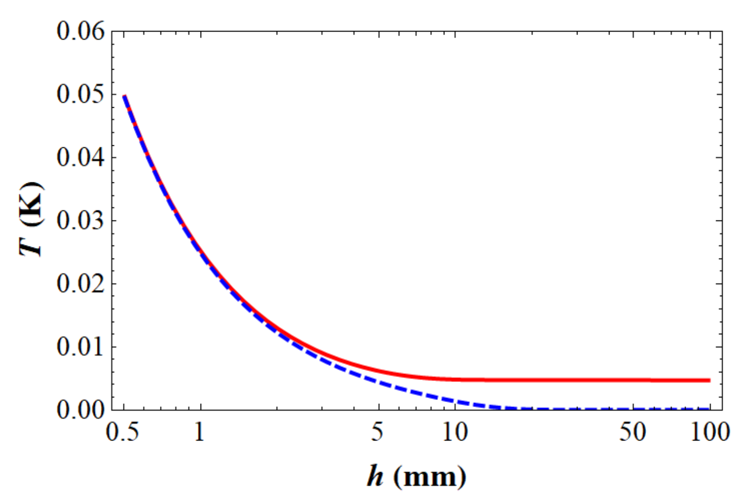
We estimated above that the adiabatic temperature increase ∆Tad could be in the range of 30 K just due to the exothermic heat of polymerization during the recording interval. As such, a high temperature increase would change the kinetic reaction constants dramatically and influence the diffusion of the monomers during grating formation. It would be interesting to estimate the realistic temperature increase taking into account the heat diffusion into the glass substrate. In addition, if the grating was formed at 30 K above the readout temperature later on there would be a large amount of Bragg detuning due to the finite CTE of the photopolymer. In the sections above we developed all the tools to estimate the realistic temperature increase in the photopolymer layer now. Again, here we focus on the isolated, non-heated surface as before, using Equation (14) and R = 600/2 mm. In Figure 15 the temperature increase at the heated and non-heated surface of the float glass is shown in dependence of h for our standard exposure time of texp = 100 s at texp.
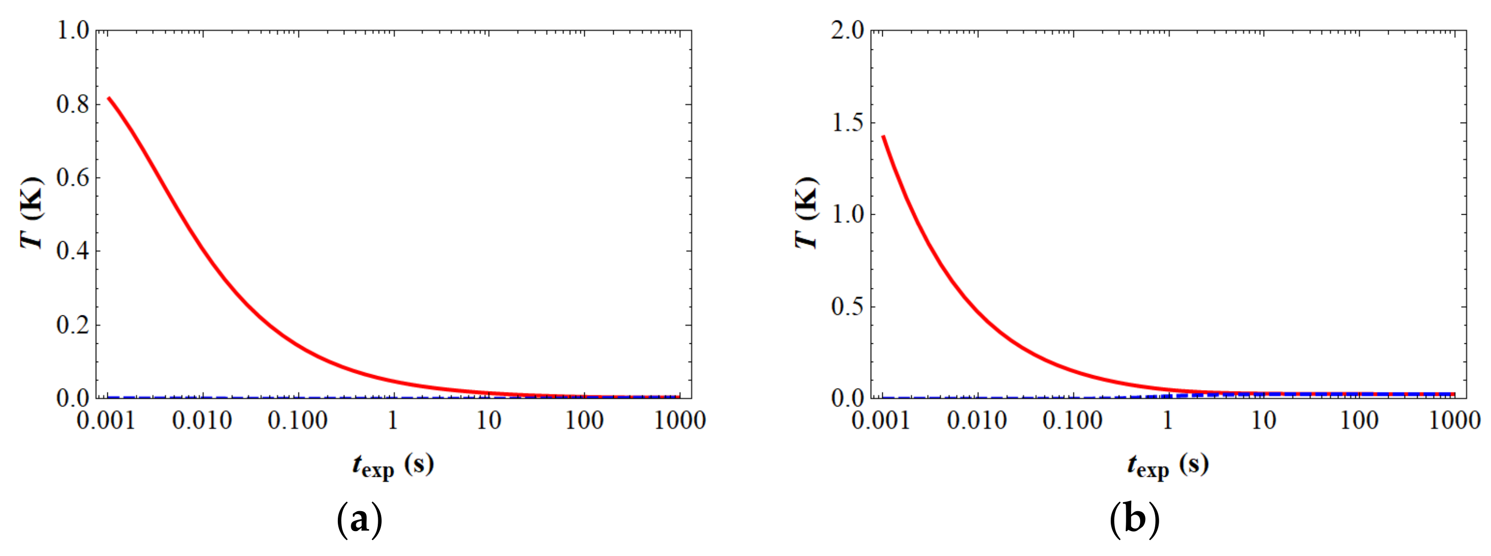
In this case, the expected increase in the temperature is less than 0.05 K at the heated side, which will be uncritical. In Figure 16 the temperature increase at the heated and non-heated surface of the float glass is shown in dependence of texp for h = 10 mm and h = 1 mm.
We can achieve ~1 K temperature increase at the heated surface if we record with power densities/exposure times which are typical for holographic CW-Laser operated printers. Therefore, for holographic CW-Laser printing the possibility of heating the photopolymer layer during recording has to be carefully considered, even if plate bending due to the small fill factor will not be a problem. However, at an exposure time of texp = 1 s the temperature increase is well below 0.1 K in both cases.
8. A Quantitative Model for Thermal Fringe Formation
In a holographic recording of an object with a plane or spherical reference wave, a main direction of the object and the reference wave can be identified. If we treat these main directions as interferences of two plane waves, the resulting normalized interference pattern of these two plane waves can be described as:
is the grating vector of this carrier interference fringe of the HOE and is formed as the difference of the wave vector of the main reference plane wave vector and the main object plane wave vector [16]. Its modulus is , whereas Λ is the carrier fringe period. V0 is the fringe visibility of the interference pattern. V0 is equal to 1 if the reference wave and the object wave have the same power density and the same polarization. If this is not the case, V0 is in the range between 0 and 1. If nothing moves during the exposure of this interference pattern to the photopolymer layer, an exact copy of this interference pattern is stored in the photopolymer layer with a maximum refractive index modulation Δnmax:
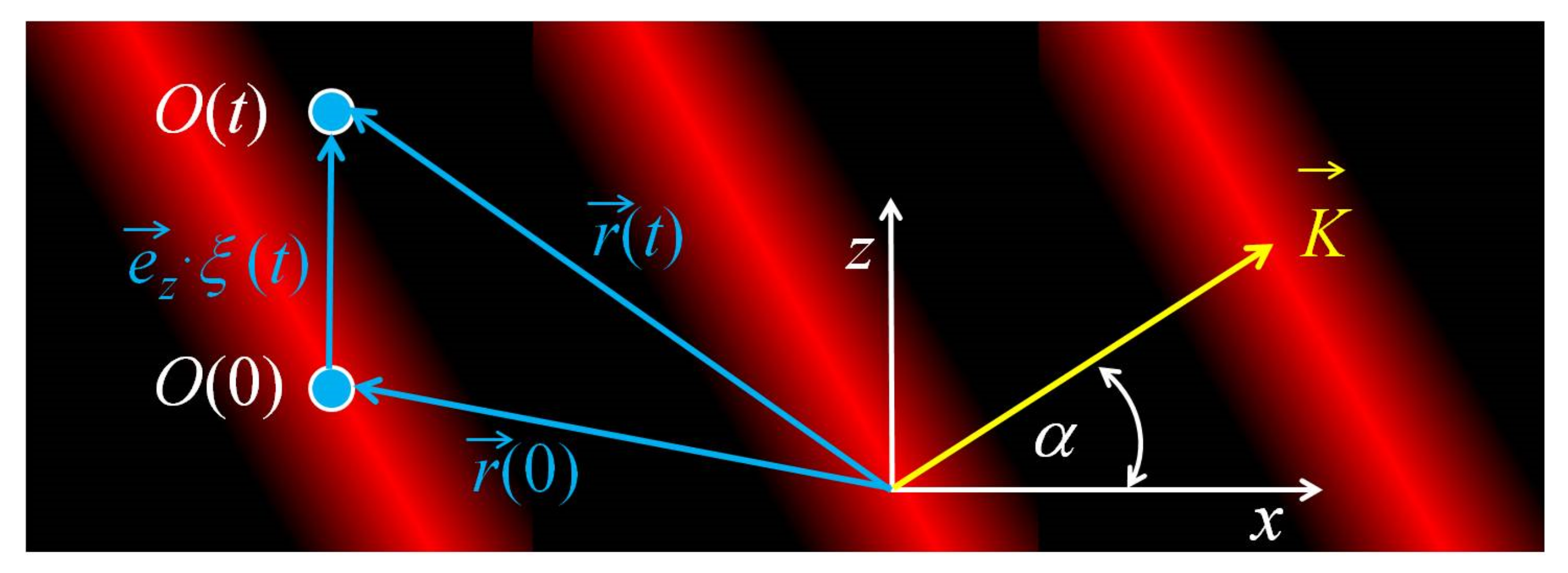
This is because the point O at the position in the photopolymer medium experiences a stationary phase Φ of this interference pattern (see Figure 17). In a dry photopolymer the grating formation is triggered by the photopolymerization of points O located in the bright fringe of the interference pattern. This means if O is located in the bright interference fringe of the interference pattern it experiences the stimulus for grating formation during the full exposure interval of duration texp.
8.1. Interference Fringe Pattern in a Bending Recording Element
If the point O however is moved due to the bending ξ(t) of the disc along the z-axis, (see also Figure 17) the transient interference pattern for the point O can be expressed as:
From Equation (26) it is obvious that the visibility of the original grating is reduced by a factor of for the point O and that in addition the point O sees the by π/2 phase shifted interference pattern.
As O was assumed to be located originally in the bright interference fringe of the carrier grating (), the phase shifted grating is that of the dark interference fringe. It will not contribute to the formation of the index modulation Δn of the hologram as no polymerization is trigged in the dark interference fringe. Therefore, the effective transient interference pattern can be assumed to be in the form:
8.2. Index Modulation in a Bending Recording Element
The form of the interference pattern in Equation (27) is now responsible for the formation of the index modulation Δn in the photopolymer which at the end represents the recorded hologram. As the fringe visibility of this pattern is not any more stationary for each point in the photopolymer layer if the recording element bends under the interaction with the recording light, the question arises as how to translate the transient visibility into the finally formed index modulation Δn. From reaction–diffusion modelling of the plane wave–plane wave recording mechanism in dry photopolymers [14] and the experimental results of plane wave–plane wave recordings [17], we can assume in a good approximation that the final index modulation Δn is linearly related to the fringe visibility V of the interference pattern during the exposure interval of duration texp.
Δnmax is the index modulation that can be achieved with a stationary non-bending recording element and at a fringe visibility V0 = 1. Knowing the relation between the fringe visibility V of the recording interference pattern and Δn given in Equation (28), it is obvious that for a bending recording element we have to consider the time averaged visibility according to Equation (29) during the exposure interval texp. The average fringe visibility V at each location of the bending recording element is given in dimensionless coordinates:
Equation (29) cannot be interpreted so easily. However, as ξ is a monotonically increasing function of the reduced time τ it has at least to reach the critical value of as otherwise the cosine function will not change its polarity.
8.3. Diffraction Efficiency η in a Bending Recording Element
To close this section, we still have to formulate the expression for the diffraction efficiency η For ηT of a transmission hologram [16], we set:
Assuming S-polarized light for the readout, and ηT = 1 if no bending of the recording element occurs, this would mean V = 1 and . For a reflection hologram [16] we set the diffraction efficiency ηR as:
8.4. The Panel-HOE (P-HOE)
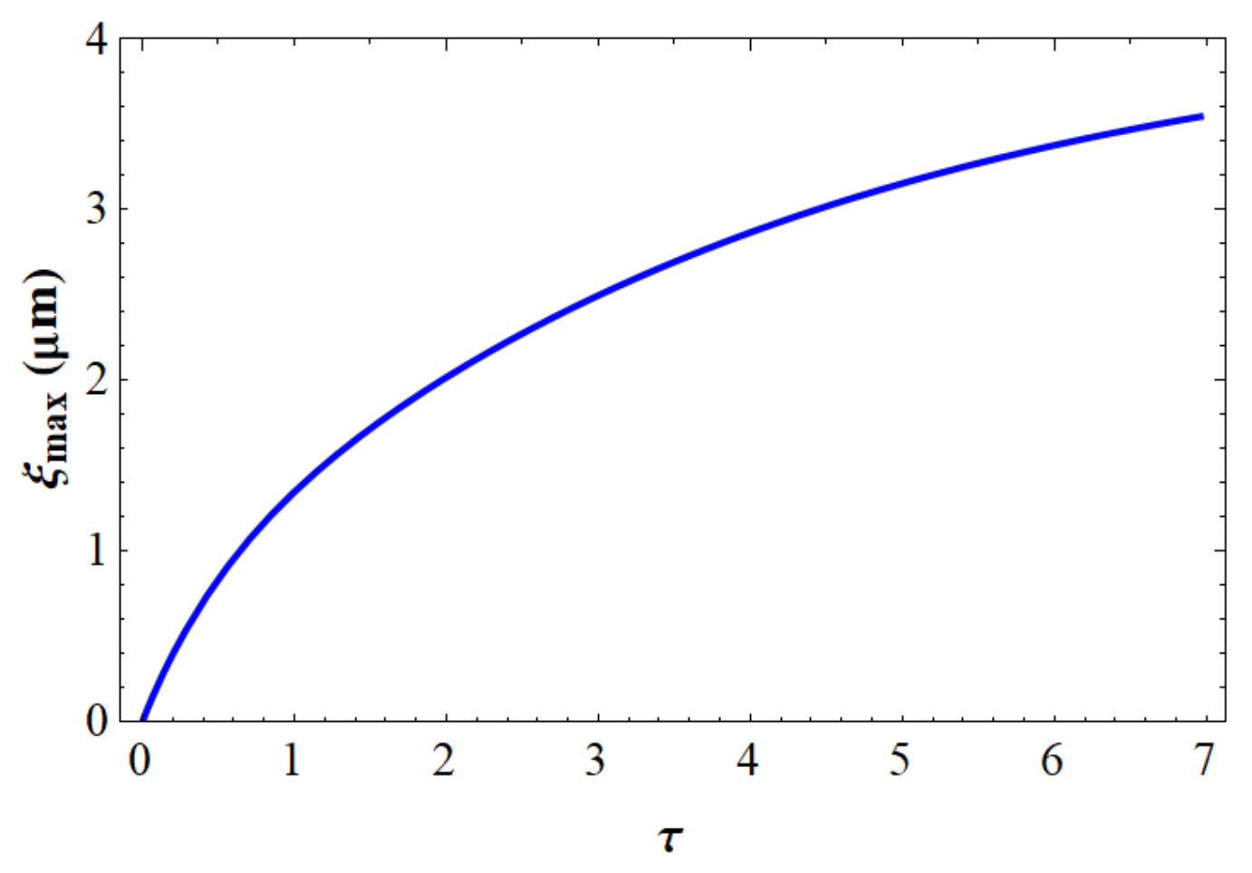
The wavelength of λ = 0.532 µm was used for the recording. If we take the average index of refraction of the photopolymer as 1.5, we can find Λ = 1.049 µm and the slant angle α = 9.7°. The thickness of the float glass plate was h = 10 mm and using the longest extension of the plate (H = 600 mm) allows for R = 600/2 mm. The CTE of the float glass is taken from Table 1 as 7 ppm/K. The typical exposure time was texp = 200 s, whereas τ0 for a float glass of the specified thickness h is 28.66 s (see Table 3) and therefore τexp = 6.98. The fixation of the recording element was completed only by three pins in a solid iron frame. Therefore, we chose the supported case for the bending deformation of the recording element. We chose the isothermal boundary condition for the non-heated surface. First, we calculated the absolute value of the bending deformation ξmax over the exposure interval in the center ( = 0) of the recording element to obtain an idea of the magnitude of the bending deformation.
The result is depicted in Figure 18.
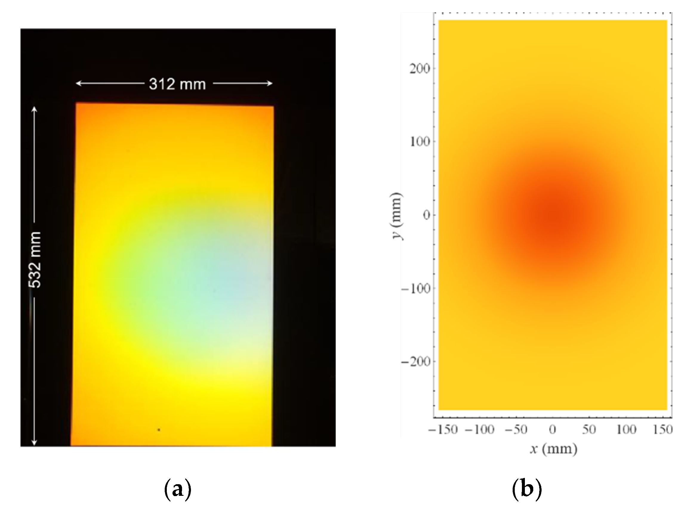
The final bending deformation in the center of the recording element is more than 3.5 µm. We then compared the diffraction efficiency ηT according to the effective visibility of the interference pattern formed by the recording beams. If we use the expression given in Equation (29) for the time averaged fringe visibility V we obtained for the diffraction efficiency ηT at each position and at τexp the Equation (33) below:
The experiment and prediction of our physical model according to Equation (31) are compared in Figure 19. Note that the eye perceives brightness on a logarithmic scale. This logarithmic scale did not apply on our simulation results. However, the experiment and prediction coincide excellently.
Using a 19 mm thick float glass plate for the P-HOE recording and also a lower power density P (increasing the texp from 200 s to 300 s) the fringe almost completely disappeared. If we used a thicker support in our model with a thickness of the glass plate h = 19 mm, τ0 for the float glass would then be 103 s (see Table 3). If we increased texp to 300 s by reducing the power density we obtain τexp = 2.88. The ratio R2/h2 will decrease by a factor of 3.6. From this, at the end the residual plate deformation will decrease clearly and from this the thermal fringe will decrease. We find in this case:
Figure 20 shows again the comparison of the experimental result and the model predictions. Moreover, it is noteworthy that we did not use any fitting parameter, which indicates that our model is able to make quantitatively correct predictions.
8.5. The Beam Shaping-HOE Master Hologram (B-HOE)
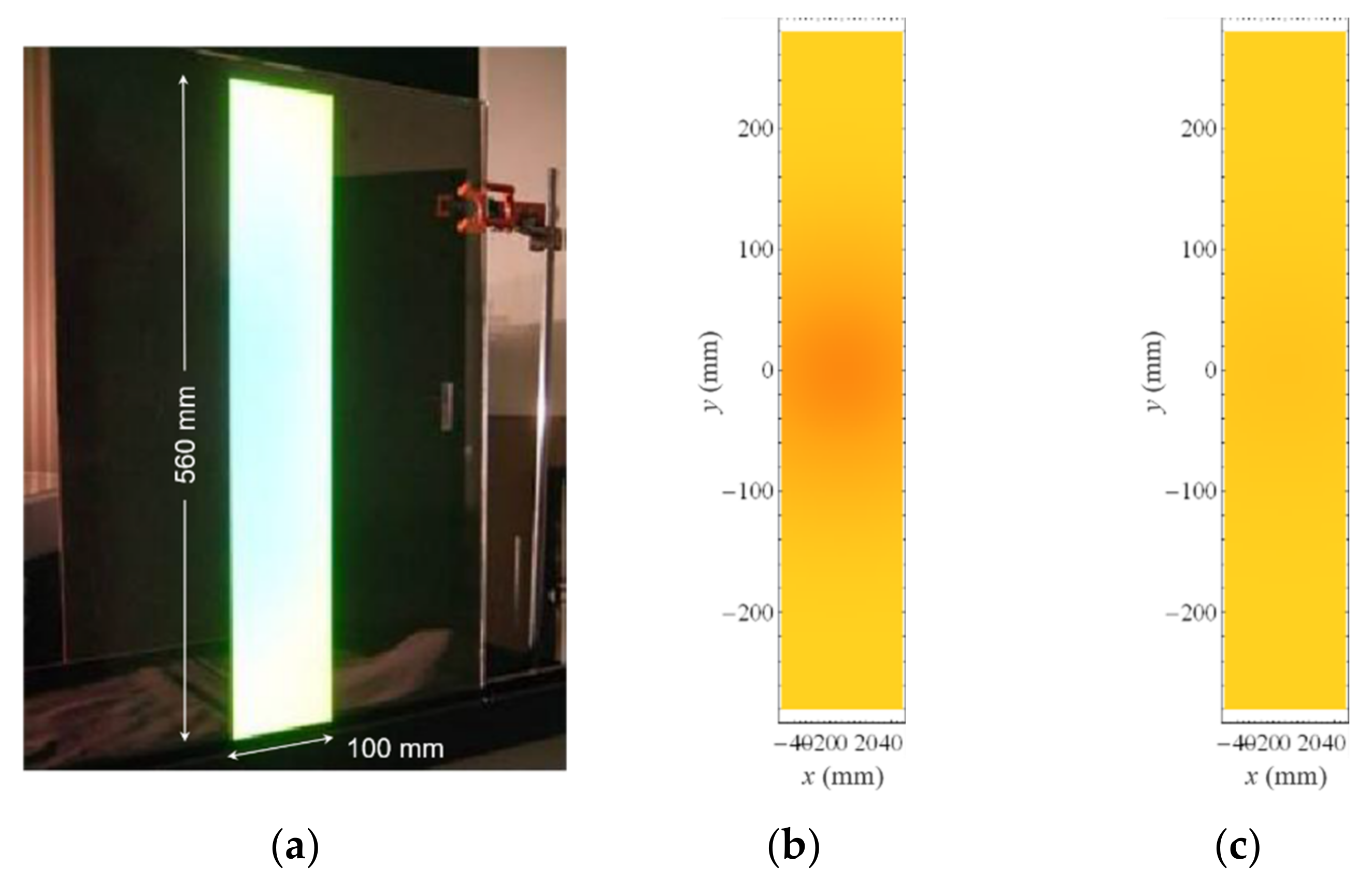
The wavelength of λ = 0.532 µm was used for recording. If we take the average index of refraction of the photopolymer as 1.5 we can find Λ = 0.567 µm and the slant angle α = 1.2°. The thickness of the float glass plate was set to h = 3 mm in this experiment and otherwise the measurements were the same as above. The exposure time was set to texp = 200 s again. τ0 for the float glass was then 2.605 s (see Table 3) and therefore τ = 76.8. We then find:
If we simulated the same recording using a 10 mm thick float glass plate, as in the exposure of the P-HOE the ratio R2/h2 will decrease by a factor of 11.1. Therefore, the increase in the ratio factor between the plate radius and plate thickness is almost completely compensated by the decrease in τexp to 6.98. From this, at the end the residual plate deformation will not change too much and also the ηsupported,isothermal;T will not change too much. We find in this case:
We found no (h = 10 mm) or only very slight (h = 3 mm) fringe formation in the simulation which is in excellent agreement with the experimental result. In Figure 21 we show the comparison of the experimental result and the model predictions.
8.6. The Beam Shaping-HOE Copy Hologram (BS-HOE)
The BS-HOE is a reflection hologram generated by a two-beam copy process from the B-HOE master hologram. In this copy process the boundary conditions for the plate fixation were more similar to the clamped case rather than the supported case, as the copy plate lies directly on the master hologram plate. The wavelength of the recording light λ was 0.532 µm. If we take the average index of refraction of the photopolymer as 1.5 we can find for Λ = 0.181 µm and for the slant angle α = 84.2°. The thickness of the glass plate was h = 10 mm and otherwise the measurements were the same as above. Again, a typical exposure time is texp = 200 s. We can assume that without fringe formation the grating strength would be large enough to maximize the efficiency η supported,isothermal;R. This gives:
The factor inside the cosine function in Equation (37) is quite large now. Even if we have the less sensitive clamped boundary conditions for the plate fixation we can expect strong fringes in the BS-HOE. Actually, we could observe these fringes experimentally (see Figure 6). To exactly fit the number of fringes seen in the experiment to the number of fringes in the simulation we had to reduce f(texp) from 0.5 to 0.17 meaning changing 9.451 in Equation (37) to 3.051 which would be equivalent for a smaller conversion. In a subsequent experiment we used Nextrema® plates instead of float glass, but with the same lateral dimensions R and the smaller thickness h = 6 mm (see Table 1) we found for τ0 = 4.62 s. Therefore τexp = 43.3. With f(texp) = 0.5 again this results in:
Now the factor in the cosine function decreases almost 30 times. Indeed, using these Nextrema® glass plates removed the fringes in the BS-HOE completely in the experiment and simulation. The comparison between the experiment and model predictions is shown in Figure 22.
Overall, the developed physical model predicted all experimental observations with respect to fringe formation with a high accuracy.
It was speculated in the past that fringe formation is also caused by the Gaussian intensity profile of the recording beams, which influences the recording in a circular symmetric but nonhomogeneous way over the exposed area. The roll off of the intensity profile in largely expanded beams can be avoided only via a big waste of laser power especially at a large HOE recording. However, it is important to rationalize that according to the model, fringe formation occurs even if the Gaussian intensity profile of the recording beams is completely flat. Experimentally we found that fringe formation happens irrespective if large size HOEs are recorded with a completely flat beam profiles or if Gaussian beam profiles are recorded with a roll off of more than 50%. Remembering our experience with a reduced fringe formation at a smaller filling factor, a Gaussian beam profile could even be advantageous in terms of reducing the fringe formation as the heating of the plate does not happen at the same time across the fully exposed area.
In case of contact, copy recording the copy film and the master hologram are usually attached to the same glass plate. Therefore, if this glass plate bends under the one-sided heating of the copy plate, the interference pattern should not move with respect to a point located in the photopolymer layer of the copy film. However, the curvature of the interference pattern will certainly change. Whether this could also have a negative effect on the brightness of the copy hologram should be investigated in a forthcoming study.
9. Conclusions
By careful analysis of the results of dedicated experiments on fringe formation in large size two beam HOE recordings in a dry photopolymer we were able to narrow down the route cause to a recording plate deformation that results from a one-sided heating of that recording plate. We rationalized that this heating was mainly caused by the heat of polymerization in the recoding medium.
Based on this, we developed for the first time a very powerful physical model (implemented in Mathematica [18]) that describes quantitatively the thermal fringe formation in large size HOE recordings into dry photopolymers. All relevant aspects were correctly included, such as photopolymer properties (heat of polymerization), recording plate geometry (size and thickness), recording parameters (power density, exposure time, plate fixation), HOE recording geometry (slant angle, transmission or reflection geometry) and support plate properties (CTE, thermal diffusion coefficient, Poisson ratio). The most powerful means to reduce the risk of fringe formation is to use glass support plates with an extremely low CTE. Having this physical model now developed and implemented allows two beam HOE recordings with an uncompromised homogeneous diffraction efficiency.
Author Contributions
Conceptualization, F.-K.B.; methodology, F.-K.B.; validation, F.-K.B., T.F. and T.R.; formal analysis, F.-K.B. and T.R.; investigation, F.-K.B., T.F. and T.R.; writing—original draft preparation, F.-K.B.; writing—review and editing, F.-K.B. and T.R.; visualization, F.-K.B. and T.R.; supervision, F.-K.B. All authors have read and agreed to the published version of the manuscript.
Funding
This research received no external funding.
Institutional Review Board Statement
Not applicable.
Informed Consent Statement
Not applicable.
Data Availability Statement
Data is contained within the article.
Acknowledgments
All the experimental holographic recordings were performed at the holographic laboratory of the Ecole Nationale Superieure de Physique Strasbourg (ENSPS) with the great help of Dalibor Vukicevic.
Conflicts of Interest
The authors declare no conflict of interest.
Appendix A
We first assume that T(z; t) is an even function in . Than we can expand the solution T(z; t) and the distribution δ(z) in a Fourier series of cosine functions as follows:
Note that the cosine function guarantees that the boundary condition at z = h in Equation (11) (thermally isolated surface) is fulfilled identically.
The Fourier coefficients bn are defined as [19]:
Therefore, we have:
Having this solved and with the help of Equation (13) we can define differential equations in time for the an(t). Note that we introduce the thermal diffusion (or relaxation) time :
Still, we have the option to use a time dependent function A(t) but for the moment we take it as a constant A. Then we can write:
At this stage the solution looks like this:
To identify the integration constants cn we have to consider the initial conditions T(z; 0). In our case this is a constant Φ.
Again, we use the identities given in [19] and find:
Inserting all cn and setting Φ = 0 we finally obtain the solution depicted in Equation (14).
Appendix B
Again we assume that T(z; t) is an even function in [−h, h]. Than we can expand the solution T(z; t) and the distribution δ(z) in a Fourier series of cosine functions as follows:
Note that the cosine function guarantees that the boundary condition at z = h in Equation (12) (isothermal surface) is fulfilled identically.
Consequently, we find for the an(t) with again τ0 = h2/(D·π2):
At this stage the solution looks like this:
To identify the integration constants cn we have to consider the initial conditions T(z; 0). In our case this is a constant Φ.
Again, we use the identities given in [19] and find:
Inserting all cn and setting Φ = 0 we finally obtain the solution depicted in Equation (16).
References
- IAA 2021 Innovation: WayRay Brings Immersion Experience to Holographic True Augmented Reality via New Deep Reality Display® System. Available online: https://wayray.com/press-releases/IAA-2021 (accessed on 26 November 2021).
- Ceres Holographic Optical Elements (HOEs) Enable New Transparent Display (TD) and Augmented Reality (AR) Applications That Transform How We See the World around Us. Available online: https://www.ceresholographics.com (accessed on 26 November 2021).
- Nakamura, T.; Tanaka, A.; Kaneko, T.; Iwasaki, M.; Kurihara, T.; Kato, N.; Kuramato, K.; Takanashi, H.; Nakahata, Y. Cylindrical Transparent Display with Hologram Screen. In Proceedings of the 26th International Display Workshops (IDW ′19), Sapporo, Japan, 27–29 November 2019. [Google Scholar]
- Yoshida, T.; Tokuyama, K.; Takai, Y.; Tsukuda, D.; Kaneko, T.; Suzuki, N.; Anzai, T.; Yoshikaie, A.; Akutsu, K.; Machida, A. A plastic holographic waveguide combiner for light-weight and highly-transparent augmented reality glasses. J. Soc. Inf. Disp. 2018, 26, 280–286. [Google Scholar] [CrossRef]
- Graf, T. Curved holographic optical elements from a geometric view point. Opt. Eng. 2021, 60, 035102. [Google Scholar] [CrossRef]
- Cakmakci, O.; Qin, Y.; Bosel, P.; Wetzstein, G. Holographic pancake optics for thin and lightweight optical see-through augmented reality. Opt. Express 2021, 29, 35206–35215. [Google Scholar] [CrossRef] [PubMed]
- Maimone, A.; Wang, J. Holographic optics for thin and lightweight virtual reality. ACM Trans. Graph. 2020, 39, 67. [Google Scholar] [CrossRef]
- Zhao, J.; Chrysler, B.D.; Kostuk, R.K. Design of a waveguide eye-tracking system operating in near-infrared with holographic optical elements. Opt. Eng. 2021, 60, 085101. [Google Scholar] [CrossRef]
- Hwang, Y.S.; Bruder, F.; Fäcke, T.; Kim, S.C.; Walze, G. Time-sequential autostereoscopic 3-D display with a novel directional backlight system based on volume-holographic optical elements. Opt. Express 2014, 22, 9820–9838. [Google Scholar] [CrossRef] [PubMed]
- Bruder, F.; Faecke, T.; Roelle, T. The Chemistry and Physics of Bayfol® HX Holographic Photopolymer. Polymers 2017, 9, 472. [Google Scholar] [CrossRef] [PubMed] [Green Version]
- Bruder, F.K.; Frank, J.; Hansen, S.; Lorenz, A.; Manecke, C.; Meisenheimer, R.; Mills, J.; Pitzer, L.; Pochorovski, I.; Rölle, T. Expanding the property profile of Bayfol® HX film towards NIR recording and ultra-high index modulation. In Optical Architectures for Displays and Sensing in Augmented, Virtual, and Mixed Reality (AR, VR, MR) II; SPIE: Bellingham, WA, USA, 2021; Volume 11765, p. 117650J. [Google Scholar]
- Landau, L.D.; Lifschitz, E.M. Theoretische Physik, Vol. VII, Elastizitätstheorie, 7th ed.; Akademie: Leipzig, Germany, 1991. [Google Scholar]
- Bruder, F.; Haese, W. Water absorption and transient tilt of polymeric substrates for optical data storage media. Jpn. J. Appl. Phys. 1999, 38, 1709. [Google Scholar] [CrossRef]
- Berneth, H.; Bruder, F.; Fäcke, T.; Hagen, R.; Hönel, D.; Jurbergs, D.; Rölle, T.; Weiser, M.S. Holographic recording aspects of high-resolution Bayfol® HX photopolymer. In Proceedings of the SPIE OPTO, San Francisco, CA, USA, 22–27 January 2011; Volume 7957, p. 79570H. [Google Scholar]
- Crank, M. The Mathematics of Diffusion, 2nd ed.; Oxford University Press: Oxford, UK, 1975. [Google Scholar]
- Hariharan, P. Optical Holography, 2nd ed.; Cambridge University Press: Cambridge, UK, 1996. [Google Scholar]
- Berneth, H.; Bruder, F.; Fäcke, T.; Hagen, R.; Hönel, D.; Rölle, T.; Walze, G.; Weiser, M.S. Holographic recordings with high beam ratios on improved Bayfol® HX photopolymer. In Holography: Advances and Modern Trends III; SPIE: Bellingham, WA, USA, 2013; Volume 8776, p. 877603. [Google Scholar]
- Mathematica; Version 7; Wolfram Research Inc.: Champaign, IL, USA, 2008.
- Boas, M.L. Mathematical Methods in the Physical Science, 2nd ed.; Wiley: New York, NY, USA, 1983. [Google Scholar]
Figure 1.
Schematic view of the P-HOE two-beam recording setup.

Figure 2.
Schematic view of the B-HOE two-beam recording setup.

Figure 3.
Schematic view of the BS-HOE two-beam close distance copy setup.

Figure 4.
(a) A P-HOE in which the photopolymer was laminated on top of a 10 mm glass. (b) The result of a repeated recording. However, in this case the photopolymer was sandwiched between two 10 mm thick glass plates.
Figure 4.
(a) A P-HOE in which the photopolymer was laminated on top of a 10 mm glass. (b) The result of a repeated recording. However, in this case the photopolymer was sandwiched between two 10 mm thick glass plates.

Figure 8.
(a) The deformation dclamped versus the normalized radial coordinate . (b) The deformation dsupported versus the normalized radial coordinate for a Poisson ratio σ = 0.3 (red line) and σ = 0.2 (blue dashed line).
Figure 8.
(a) The deformation dclamped versus the normalized radial coordinate . (b) The deformation dsupported versus the normalized radial coordinate for a Poisson ratio σ = 0.3 (red line) and σ = 0.2 (blue dashed line).

Figure 9.
(a) The temperature profile Θisolated(; τ) at values of τ = 0.1, 0.5, 1, 2 and 5. (b) The transient behavior of Γisolated(τ).
Figure 9.
(a) The temperature profile Θisolated(; τ) at values of τ = 0.1, 0.5, 1, 2 and 5. (b) The transient behavior of Γisolated(τ).

Figure 10.
(a) The temperature profile Θisothermal(ζ; τ) at values of τ = 0.1, 1, 5, 10, and 20. (b) The transient behavior of Γisothermal(τ) as blue line. For comparison Γisolated(τ) is given as a red line in this plot.
Figure 10.
(a) The temperature profile Θisothermal(ζ; τ) at values of τ = 0.1, 1, 5, 10, and 20. (b) The transient behavior of Γisothermal(τ) as blue line. For comparison Γisolated(τ) is given as a red line in this plot.

Figure 11.
This plot shows the behavior of as a blue line and for comparison is shown as a red line.
Figure 11.
This plot shows the behavior of as a blue line and for comparison is shown as a red line.

Figure 12.
This plot shows |ξmax| in dependence of h, at a fixed exposure time texp and R for float glass (red line) and Nextrema® (blue line).
Figure 12.
This plot shows |ξmax| in dependence of h, at a fixed exposure time texp and R for float glass (red line) and Nextrema® (blue line).

Figure 13.
This plot shows ξmax in dependence of texp at fixed thickness h and R for float glass (red line, h = 10 mm) and Nextrema® (blue line, h = 6 mm).
Figure 13.
This plot shows ξmax in dependence of texp at fixed thickness h and R for float glass (red line, h = 10 mm) and Nextrema® (blue line, h = 6 mm).

Figure 14.
|ξmax| versus and .

Figure 15.
Temperature increase versus h at the heated surface at z = 0 (red line) and the non-heated surface z = h (blue dashed line) of the supporting float glass. texp = 100 s is fixed.
Figure 15.
Temperature increase versus h at the heated surface at z = 0 (red line) and the non-heated surface z = h (blue dashed line) of the supporting float glass. texp = 100 s is fixed.

Figure 16.
Temperature increase T versus texp at the heated surface at z = 0 (red line) and the non-heated surface z = h (blue dashed line) of the supporting float glass. h = 10 mm (a) and h = 1 mm (b).
Figure 16.
Temperature increase T versus texp at the heated surface at z = 0 (red line) and the non-heated surface z = h (blue dashed line) of the supporting float glass. h = 10 mm (a) and h = 1 mm (b).

Figure 17.
Change of the phase of the point O during plate bending.

Figure 18.
Transient behavior of ξmax (blue line).

Figure 19.
(a) diffraction efficiency for the P-HOE reconstructed with slightly divergent white light source. (b) model predictions. A 10 mm thick float glass plate was used for the recording element.
Figure 19.
(a) diffraction efficiency for the P-HOE reconstructed with slightly divergent white light source. (b) model predictions. A 10 mm thick float glass plate was used for the recording element.

Figure 20.
(a) diffraction efficiency for the P-HOE. (b) model predictions. A 19 mm thick float glass plate was used for the recording element and the power density was reduced by a factor of 1.5.
Figure 20.
(a) diffraction efficiency for the P-HOE. (b) model predictions. A 19 mm thick float glass plate was used for the recording element and the power density was reduced by a factor of 1.5.

Figure 21.
(a) diffraction efficiency for the B-HOE recorded on a 3 mm thick glass plate. (b) model predictions for a 3 mm thick float glass plate. (c) model predictions for a 10 mm thick float glass plate.
Figure 21.
(a) diffraction efficiency for the B-HOE recorded on a 3 mm thick glass plate. (b) model predictions for a 3 mm thick float glass plate. (c) model predictions for a 10 mm thick float glass plate.

Figure 22.
(a) diffraction efficiency for the BS-HOE recorded on a 10 mm thick glass plate and reconstructed with divergent laser light of λ = 0.488 µm. (b) model predictions for a 10 mm thick float glass plate with f(texp) adapted. (c) model predictions for a 6 mm thick Nextrema® plate.
Figure 22.
(a) diffraction efficiency for the BS-HOE recorded on a 10 mm thick glass plate and reconstructed with divergent laser light of λ = 0.488 µm. (b) model predictions for a 10 mm thick float glass plate with f(texp) adapted. (c) model predictions for a 6 mm thick Nextrema® plate.


Table 1.
Thermal material properties. Nextrema® is a trademark of Schott Glas, Germany.
| Layer Material | ΛT (W/m·K) | cP (J/cm3·K) | D (cm2/s) | Layer Thickness (µm) | τ0 (s) | CTE (ppm/K) |
|---|---|---|---|---|---|---|
| Substrate | 0.2 | 2 | 0.001 | 50 | 0.0025 | 60 |
| Photopolymer | 0.2 | 2 | 0.001 | 15 | 0.0002 | 250 |
| Float glass support | 0.76 | 2.15 | 0.0035 | 10,000 | 28.66 | 7 |
| Nextrema® glass support | 1.6 | 2.032 | 0.0079 | 6000 | 4.62 | −0.54 |
Table 2.
Further specific material properties.
| Layer Material | ΔHP (J/cm3) | Tini (%) | σ | G (MPa) |
|---|---|---|---|---|
| Substrate | ~0.4 | ~660–1000 | ||
| Photopolymer | ~133 + | ~40 | 0.5 */20 ** | |
| Float glass support | 0.3 | 10000 | ||
| Nextrema® glass support | 0.25 | 6000 |
* Before exposure, ** fully cured, + estimated from the heat of polymerization of an acrylate group of ~604 J/g and the amount of acrylate groups in the Bayfol® HX development grade at full conversion.
Table 3.
Variation of the disc thickness h for float glass, R = 600/2 mm and texp = 100 s.
| h (mm) | 0.5 | 1 | 3 | 10 | 19 | 30 |
|---|---|---|---|---|---|---|
| τ0 (s) | 0.072 | 0.27 | 2.6 | 29 | 103 | 258 |
| τexp | 1389 | 370 | 39 | 3.5 | 0.97 | 0.39 |
| Γisolated(τexp)/τexp | 0.00071 | 0.0027 | 0.026 | 0.28 | 0.66 | 0.86 |
| R2/h2 | 360000 | 90000 | 10000 | 900 | 249 | 100 |
| ξmax (µm) | 0.56 | 0.56 | 0.56 | 0.54 | 0.35 | 0.18 |
Table 4.
Variation of the disc thickness h for float glass, R = 120/2 mm and texp = 100 s.
| h (mm) | 0.5 | 1 | 3 | 10 | 19 | 30 |
|---|---|---|---|---|---|---|
| τ0 (s) | 0.072 | 0.27 | 2.6 | 29 | 103 | 258 |
| τexp | 1389 | 370 | 39 | 3.5 | 0.97 | 0.39 |
| Γisolated(τexp)/τexp | 0.00071 | 0.0027 | 0.026 | 0.28 | 0.66 | 0.86 |
| R2/h2 | 14,400 | 3600 | 400 | 36 | 10 | 4.0 |
| ζmax (µm) | 0.022 | 0.022 | 0.022 | 0.022 | 0.014 | 0.0074 |
Table 5.
Variation of the exposure time texp for float glass, R = 600/2 mm and h = 10 mm.
| texp (s) | 0.001 | 0.01 | 0.1 | 1 | 10 | 100 | 1000 |
|---|---|---|---|---|---|---|---|
| τ0 (s) | 29 | 29 | 29 | 29 | 29 | 29 | 29 |
| τexp | 0.000035 | 0.00035 | 0.0035 | 0.035 | 0.35 | 3.5 | 35 |
| Γisolated(τexp)/τexp | 1.22 | 1.22 | 1.20 | 1.12 | 0.87 | 0.28 | 0.029 |
| R2/h2 | 900 | 900 | 900 | 900 | 900 | 900 | 900 |
| ζmax (µm) | 2.33 | 2.33 | 2.29 | 2.15 | 1.69 | 0.54 | 0.056 |
Table 6.
Variation of the exposure time texp for float glass, R = 120/2 mm and h = 3 mm.
| texp (s) | 0.001 | 0.01 | 0.1 | 1 | 10 | 100 | 1000 |
|---|---|---|---|---|---|---|---|
| τ0 (s) | 2.61 | 2.61 | 2.61 | 2.61 | 2.61 | 2.61 | 2.61 |
| τexp | 0.000384 | 0.00384 | 0.0384 | 0.384 | 3.84 | 38.4 | 384 |
| Γisolated(τexp)/τexp | 1.22 | 1.20 | 1.12 | 0.87 | 0.26 | 0.026 | 0.0026 |
| R2/h2 | 400 | 400 | 400 | 400 | 400 | 400 | 400 |
| ζmax (µm) | 1.03 | 1.02 | 0.95 | 0.74 | 0.22 | 0.022 | 0.0022 |
Publisher’s Note: MDPI stays neutral with regard to jurisdictional claims in published maps and institutional affiliations. |
© 2021 by the authors. Licensee MDPI, Basel, Switzerland. This article is an open access article distributed under the terms and conditions of the Creative Commons Attribution (CC BY) license (https://creativecommons.org/licenses/by/4.0/).
Share and Cite
MDPI and ACS Style
Bruder, F.-K.; Fäcke, T.; Rölle, T. Thermal Fringe Formation during a Hologram Recording Using a Dry Photopolymer. Photonics 2021, 8, 589. https://doi.org/10.3390/photonics8120589
AMA Style
Bruder F-K, Fäcke T, Rölle T. Thermal Fringe Formation during a Hologram Recording Using a Dry Photopolymer. Photonics. 2021; 8(12):589. https://doi.org/10.3390/photonics8120589
Chicago/Turabian StyleBruder, Friedrich-Karl, Thomas Fäcke, and Thomas Rölle. 2021. "Thermal Fringe Formation during a Hologram Recording Using a Dry Photopolymer" Photonics 8, no. 12: 589. https://doi.org/10.3390/photonics8120589
Note that from the first issue of 2016, this journal uses article numbers instead of page numbers. See further details here.