An Infrared DoLP Model Considering the Radiation Coupling Effect

Abstract

The polarization degree of objects in the marine background are affected by infrared radiation from sea surface. Taking into account the radiation coupling effect (RCE), a degree of linear polarization (DoLP) model is deduced. The DoLP of painted aluminum plates at different observation angles are simulated. The simulation results show the trend of the DoLP of the object decreases first and then increases as the observation angle ${\theta }_O$, with the minimum value at ${\theta }_O={53}^{\circ }$. Nevertheless, we get a monotonically increasing trend and the minimum value is at ${\theta }_O=0^{\circ }$ without considering RCE. The experimental results accord closely with those of the simulation with RCE. This conclusion is useful for the polarization detection and identification of infrared objects in the marine background.

1. Introduction

Compared with traditional infrared technology, polarization detection can obtain more information, such as the degree of linear polarization (DoLP) and the angle of polarization. Infrared polarization detection technology shows a promising application prospect in the field of remote sensing [1,2,3], and object detection and identification [4,5,6,7]. However, in the long-wave infrared (LWIR) band, the object polarization characteristics are strongly influenced by environmental factors [8,9]. When the emitted radiation is close to incident radiation, the polarization degrades and even disappears [10]. For objects in the marine background, the radiation from the sea surface and surroundings can be reflected into the detector by the object’s surface, coupling with the object’s radiation. Thus, the measured polarization characteristics can be remarkably changed. The radiation coupling effect (RCE) cannot be ignored for shore-based or low-altitude infrared polarization detection and identification in a marine background.

The reflection polarization characteristics of objects are usually described by the polarization bidirectional reflection distribution function model (pBRDF) [11]. In 2000, Priest and Germer [12] developed the first strictly pBRDF model based on the T-S microfacet model [13], which extended the scalar BRDF to a polarization vector model via the Mueller matrix. Hyde [14] improved the model established by Priest and Germer, and increased the geometric attenuation factor and the diffuse reflection component, which improved the simulation accuracy of the model, resulting in a relatively complete and accurate pBRDF model. Feng [15] and Liu [16] measured the pBRDF of materials such as E235B steel using a self-designed instrument. On the basis of the pBRDF model and Fresnel’s reflection law, many researchers have conducted studies on object polarization characteristics. Jordan [17], Wolff [18] and Gurton [19] measured the DoLP of object with different degrees of roughness. In 2014, Yan [20] studied the long-wave infrared polarization characteristics of typical metallic objects such as aluminum and iron coated aluminum plates, focusing on the effect of temperature on the polarization degree. In 2016, Liu [21] analyzed and discussed the influence of spatial geometric parameters such as detection distance and object shape on the object’s DoLP. In 2017, based on a three-component assumption, Liu [22] established the pBRDF model of the coating, and used satellite coating samples sr107 and s781 as examples to simulate and measure the polarization characteristics. In 2020, Chen [23] analyzed polarization models and polarization properties of human bodies and transparent objects. Zhang [24] investigated the optical polarization characteristics of low-earth-orbit space targets; Su [25] and Tuo [26] studied the ship target detection method based on polarization characteristics. Zhang [27] and Wei [28] proposed a new detection method based on the infrared polarization feature of the object. The studies above present models of DoLP, taking into account various factors, such as materials, observation angle, surface roughness, temperature, and so on. The polarization characteristics of the target are directly used for detection and recognition. However, the DoLP models for the objects in strong radiation and reflection backgrounds, such as the marine background, are found lacking; and few studies have been carried out concerning the polarization characteristics of objects in these backgrounds.

In this paper, the DoLP of an object in the marine background is modelled by considering the RCE, based on the Hyde model of pBRDF. The influence of the RCE on the infrared polarization characteristics of the object is analyzed, and an LWIR polarization measurement system is built to measure the DoLP of the object at different temperatures and observation angles. The experimental results are consistent with the simulation ones.

2. Materials and Methods

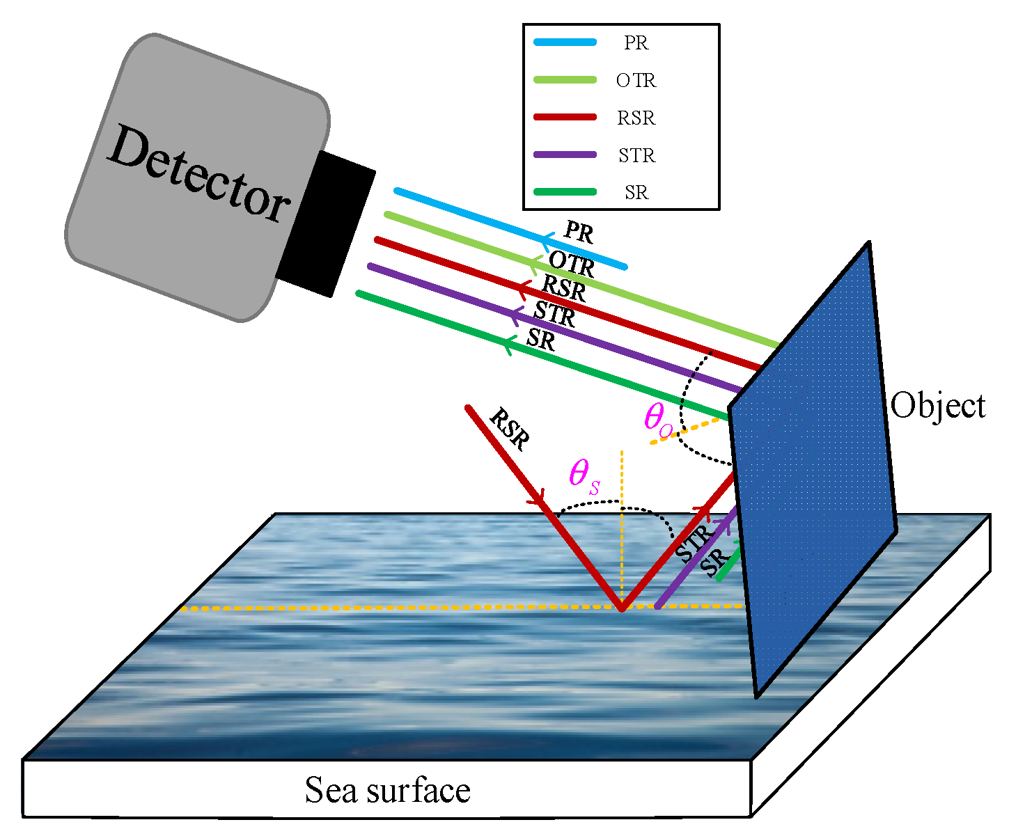
For objects in the marine background, the energy entering the detector consists of three components, i.e., the path radiation (PR) between the object and the detector, the object thermal radiation (OTR), and the reflected thermal radiation (RTR) from the object surface, including reflected surroundings radiation (RSR) from the sea surface, sea-surface thermal radiation (STR), and surroundings radiation (SR) into the object, as shown in Figure 1. Because the PR has little influence on the DoLP of object [29], only two factors are considered in the DoLP modeling, that is, the OTR and the RTR.

2.1. pBRDF Model

In this paper, a DoLP model is deduced based on the Hyde model [14], which assumes that the energy reflected by the rough surface includes specular reflection and diffuse reflection, so the pBRDF of object also includes two parts.

$$\begin{array}{ll}\mathit{f}(\theta ,{\theta }_i,{\varphi }_i,{\theta }_r,{\varphi }_r,\lambda )& ={\mathit{f}}^s+{\mathit{f}}^d\\ & =\left(\begin{array}{cccc}{f}_{00}& f_{01}& f_{02}& f_{03}\\ f_{10}& f_{11}& f_{12}& f_{13}\\ f_{20}& f_{21}& f_{22}& f_{23}\\ f_{30}& f_{31}& f_{32}& f_{33}\end{array}\right)\end{array}$$

(1)

Here, the specular reflection part ${\mathit{f}}^s$ can be obtained by micro-faced theory. When the microfacet element normal distribution satisfies the Gaussian distribution, its expression is

$${\mathit{f}}^s(\theta ,{\theta }_i,{\varphi }_i,{\theta }_r,{\varphi }_r,\lambda )=\frac{\exp (-{\tan }^2\theta /2{\sigma }^2)}{8\pi {\sigma }^2{\cos }^4\theta \cos {\theta }_i\cos {\theta }_r}G(\theta ,{\theta }_i,{\theta }_r)\mathit{M}({\theta }_i,{\theta }_r,{\varphi }_i,{\varphi }_r)$$

(2)

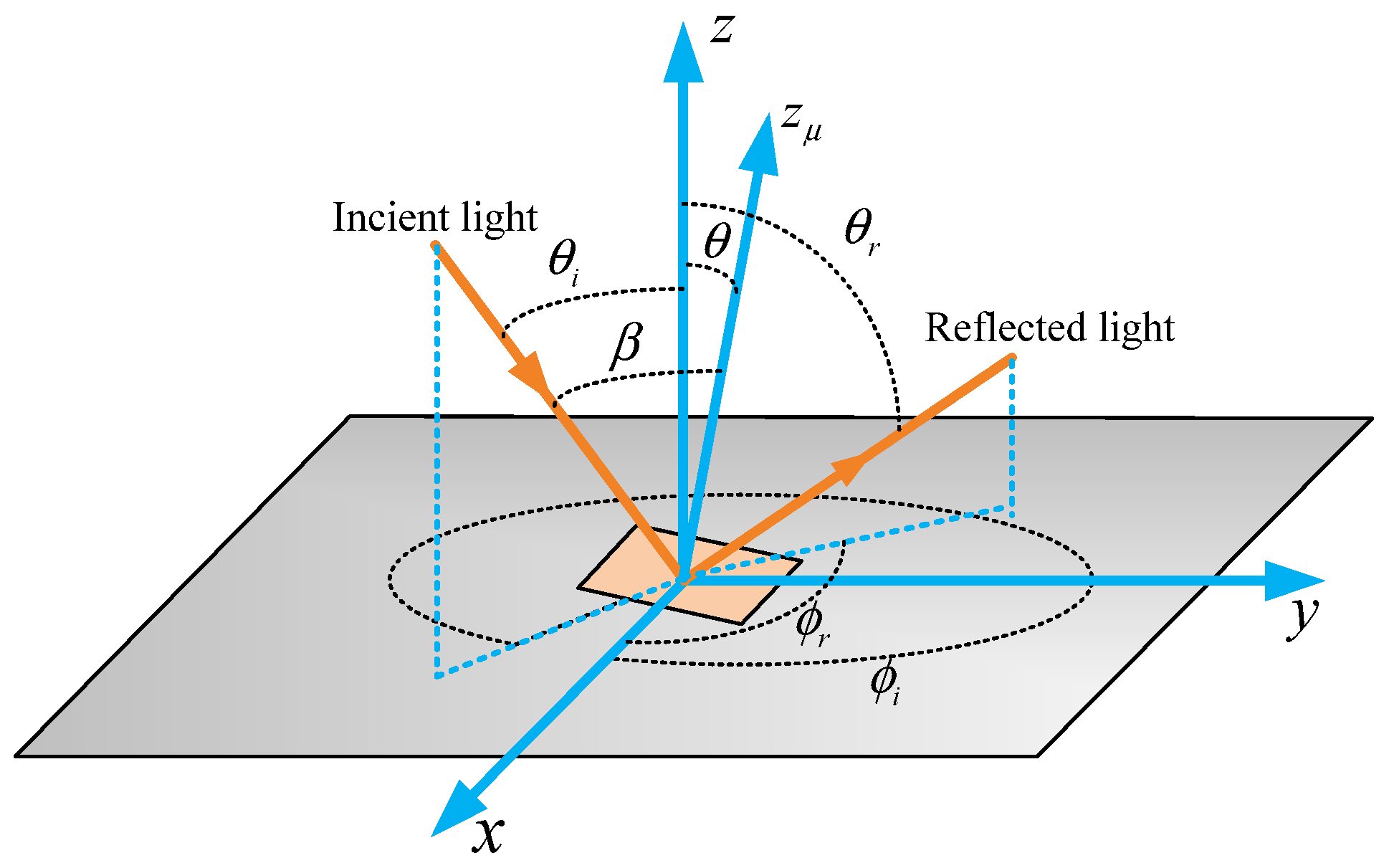
where $G(\theta ,{\theta }_i,{\theta }_r)$ is the shadowing and masking function. $\mathit{M}({\theta }_i,{\theta }_r,{\varphi }_i,{\varphi }_r)$ is a reflection Muller matrix of specular surface. ${\theta }_i$, ${\varphi }_i$, ${\theta }_r$ and ${\varphi }_r$ are the zenith and azimuth angle of incident light and reflected light, respectively, as shown in Figure 2. $\beta$ is the angle between incident light and the normal of the micro face. $\sigma$ is the slope variance of microfacet element, which is considered as surface roughness in this paper. $\theta$ is the angle between the normal of surface and the normal of the micro face. The expression of $G(\theta ,{\theta }_i,{\theta }_r)$ is as follows,

$$G(\theta ,{\theta }_i,{\theta }_r)=\min (1;\frac{2\cos \theta \cos {\theta }_r}{\cos \beta };\frac{2\cos \theta \cos {\theta }_i}{\cos \beta })$$

From the geometric relationship, the following equation can be derived

$$\{\begin{array}{l}\cos \theta =\frac{\cos {\theta }_i+\cos {\theta }_r}{2\cos \beta }\\ \cos 2\beta =\cos {\theta }_i\cos {\theta }_r+\sin {\theta }_i\sin {\theta }_r\cos ({\varphi }_r-{\varphi }_i)\end{array}$$

(3)

The specular reflection Mueller matrix $\mathit{M}({\theta }_i,{\theta }_r,{\varphi }_i,{\varphi }_r)$ can be solved by its correspondence with the Jones matrix [30].

$$\mathit{M}=\left(\begin{array}{cccc}{M}_{00}& M_{10}& 0& 0\\ M_{10}& M_{00}& 0& 0\\ 0& 0& M_{22}& j{M}_{32}\\ 0& 0& -j{M}_{32}& M_{22}\end{array}\right)$$

(4)

In which $M_{00}=\frac{R_s+R_p}{2},M_{10}=\frac{R_s-R_p}{2},M_{22}=\sqrt{R_s{R}_p}$, $R_s$ and $R_p$ represent reflectance of the s-polarized and p-polarized components, respectively, which can be calculated by Fresnel equations. For substances with complex refractive index $\tilde{n}=n+\mathrm{i}k$ [31],

$$\{\begin{array}{l}{R}_s(\beta ,\tilde{n})=\frac{{(\mathrm{A}-\cos \beta )}^2+B^2}{{(\mathrm{A}+\cos \beta )}^2+B^2}\\ R_p(\beta ,\tilde{n})=R_s\frac{{(\mathrm{A}-\sin \beta \tan \beta )}^2+B^2}{{(\mathrm{A}+\sin \beta \tan \beta )}^2+B^2}\\ \mathrm{A}=\sqrt{\frac{\sqrt{4n^2{k}^2+{\left(n^2-k^2-\sin {\beta }^2\right)}^2}+\left(n^2-k^2-\sin {\beta }^2\right)}{2}}\\ \mathrm{B}=\sqrt{\frac{\sqrt{4n^2{k}^2+{\left(n^2-k^2-\sin {\beta }^2\right)}^2}-\left(n^2-k^2-\sin {\beta }^2\right)}{2}}\end{array}$$

(5)

Here, $\beta$ is the incidence angle. The directional hemispherical reflectance (DHR) can be obtained from the pBRDF [29].

$${\rho }_{DHR}^s={\displaystyle {\int }_0^{2\mathsf{\pi }}{\displaystyle {\int }_0^{\mathsf{\pi }/2}{f}_{00}^s(\theta ,{\theta }_i,{\varphi }_i,{\theta }_r,{\varphi }_r)}}\cos {\theta }_r\sin {\theta }_{r}d{\theta }_{r}d{\varphi }_r$$

(6)

Considering that the diffuse reflection component ${\mathit{f}}^d$ is obtained after multiple reflections on the object surface and is usually non-polarized, it can be solved by the DHR and the law of energy conservation.

$$f_{00}^d({\theta }_r,{\varphi }_r)=\frac{1}{\mathsf{\pi }}(1-{\displaystyle {\int }_0^{2\mathsf{\pi }}{\displaystyle {\int }_0^{\mathsf{\pi }/2}{f}_{00}^s(\theta ,{\theta }_i,{\varphi }_i,{\theta }_r,{\varphi }_r)}}\cos {\theta }_r\sin {\theta }_{r}d{\theta }_{r}d{\varphi }_r)$$

(7)

where $f_{00}=f_{00}^s(\theta ,{\theta }_i,{\varphi }_i,{\theta }_r,{\varphi }_r)+f_{00}^d({\theta }_r,{\varphi }_r)M_{00}$. Therefore,

$$\begin{array}{ll}\mathrm{d}{\mathit{S}}_r({\theta }_r,{\varphi }_r)& =\mathit{f}\cdot \mathrm{d}{\mathit{S}}_i({\theta }_i,{\varphi }_i)\\ & =\left(\begin{array}{cccc}{f}_{00}^s+f_{00}^d{M}_{00}& f_{01}^s& f_{02}^s& f_{03}^s\\ f_{10}^s& f_{11}^s& f_{12}^s& f_{13}^s\\ f_{20}^s& f_{21}^s& f_{22}^s& f_{23}^s\\ f_{30}^s& f_{31}^s& f_{32}^s& f_{33}^s\end{array}\right)\left(\begin{array}{c}{S}_{i,0}\\ S_{i,1}\\ S_{i,2}\\ S_{i,3}\end{array}\right)\end{array}$$

(8)

Here, ${\left(\begin{array}{cccc}{S}_{i,0}& S_{i,1}& S_{i,2}& S_{i,3}\end{array}\right)}^{\mathrm{T}}$ is the Stokes vector of incident light, whose common expression is $\mathit{S}={\left(\begin{array}{cccc}{S}_0& S_1& S_2& S_3\end{array}\right)}^{\mathrm{T}}$, where $S_0$ represents the total intensity of radiation, $S_1$ represents the difference between the radiation intensities in the horizontal direction and vertical direction, and $S_2$ and $S_3$ represent the modulation relationship between the amplitude and phase of horizontal light wave and vertical light wave. In polarization detection, component $S_3$ can usually be omitted as being small. Therefore, the DoLP can be solved according to Stokes vector.

$$DoLP=\frac{\sqrt{S_1^2+S_2^2}}{S_0}$$

(9)

2.2. DoLP Model Considering the RCE

2.2.1. Reflection DoLP Model of Rough Surface

In the marine background, the energy entering the detector mainly consists of two parts: the OTR and the RTR, as shown in Figure 1. As the RCE needs to be taken into account, the RTR includes the SR, RSR and STR. Therefore, the Stokes vector of incident light can be written as,

$${\mathit{S}}_i={\mathit{S}}_{SR}+{\mathit{S}}_{RSR}+{\mathit{S}}_{STR}$$

(10)

Because the SR is non-polarized, the Equation (10) can be written as,

$$\left(\begin{array}{c}{S}_{i,0}\\ \begin{array}{l}{S}_{i,1}\\ S_{i,2}\end{array}\\ S_{i,3}\end{array}\right)=\left(\begin{array}{c}{I}_{SR}\\ \begin{array}{l}0\\ 0\end{array}\\ 0\end{array}\right)+\left(\begin{array}{c}{S}_{RSR,0}\\ \begin{array}{l}{S}_{RSR,1}\\ S_{RSR,2}\end{array}\\ S_{RSR,3}\end{array}\right)+\left(\begin{array}{c}{S}_{STR,0}\\ S_{STR,1}\\ S_{STR,2}\\ S_{STR,3}\end{array}\right)$$

(11)

Approximating the calm sea surface as an ideal mirror surface, the spontaneous STR and the RSR can be solved using Fresnel’s law of reflection.

$$\left(\begin{array}{c}{S}_{STR,0}\\ S_{STR,1}\\ S_{STR,2}\\ S_{STR,3}\end{array}\right)=\left(\begin{array}{c}\frac{1-R_{s\_S}}{2}{I}_{STR}+\frac{1-R_{p\_S}}{2}{I}_{STR}\\ \frac{1-R_{s\_S}}{2}{I}_{STR}+\frac{1-R_{p\_S}}{2}{I}_{STR}\\ 0\\ 0\end{array}\right)$$

(12)

$$\left(\begin{array}{c}{S}_{RSR,0}\\ \begin{array}{l}{S}_{RSR,1}\\ S_{RSR,2}\end{array}\\ S_{RSR,3}\end{array}\right)=\left(\begin{array}{c}\frac{R_{s\_S}{I}_{SR}}{2}+\frac{R_{p\_S}{I}_{SR}}{2}\\ \frac{R_{s\_S}{I}_{SR}}{2}-\frac{R_{p\_S}{I}_{SR}}{2}\\ 0\\ 0\end{array}\right)$$

(13)

Here, $I_{STR}$ and $I_{SR}$ represent the intensity of the STR and SR, respectively. $R_{s\_S}$ and $R_{p\_S}$ represent reflectance of the s-polarized and p-polarized components, respectively. ${\theta }_S$ and ${\tilde{n}}_S$ are incidence angle at the sea surface and complex refractive index of sea water, respectively. Therefore, ${\mathit{S}}_i$ can be expressed as follows,

$$\left(\begin{array}{c}{S}_{i,0}\\ \begin{array}{l}{S}_{i,1}\\ S_{i,2}\end{array}\\ S_{i,3}\end{array}\right)=\left(\begin{array}{c}{I}_{SR}+\frac{1-R_{s\_S}}{2}{I}_{STR}+\frac{1-R_{p\_S}}{2}{I}_{STR}+\frac{R_{s\_S}{I}_{SR}}{2}+\frac{R_{p\_S}{I}_{SR}}{2}\\ \begin{array}{c}\frac{1-R_{s\_S}}{2}{I}_{STR}-\frac{1-R_{p\_S}}{2}{I}_{STR}+\frac{R_{s\_S}{I}_{SR}}{2}-\frac{R_{p\_S}{I}_{SR}}{2}\\ 0\end{array}\\ 0\end{array}\right)$$

(14)

Then, according to Equation (8), the reflected Stokes vector of the object is,

$$\begin{array}{ll}\left(\begin{array}{c}{S}_{r,0}\\ \begin{array}{l}{S}_{r,1}\\ S_{r,2}\end{array}\\ S_{r,3}\end{array}\right)& =\left(\begin{array}{cccc}{\displaystyle \int [f_{00}^s({\theta }_r,{\varphi }_i)+f_{00}^d({\theta }_r,{\varphi }_i)M_{00}]\cos {\theta }_r}d{\mathsf{\Omega }}_r& {\displaystyle \int f_{10}^s({\theta }_r,{\varphi }_i)\cos {\theta }_r}d{\mathsf{\Omega }}_r& 0& 0\\ {\displaystyle \int f_{10}^s({\theta }_r,{\varphi }_i)\cos {\theta }_r}d{\mathsf{\Omega }}_r& {\displaystyle \int [f_{00}^s({\theta }_r,{\varphi }_i)+f_{00}^d({\theta }_r,{\varphi }_i)M_{00}]\cos {\theta }_r}d{\mathsf{\Omega }}_r& 0& 0\\ 0& 0& {\displaystyle \int f_{22}^s({\theta }_r,{\varphi }_i)\cos ({\theta }_r)}d{\mathsf{\Omega }}_r& {\displaystyle \int f_{23}^s({\theta }_r,{\varphi }_i)\cos {\theta }_r}d{\mathsf{\Omega }}_r\\ 0& 0& {\displaystyle \int f_{32}^s({\theta }_r,{\varphi }_i)\cos ({\theta }_r)}d{\mathsf{\Omega }}_r& {\displaystyle \int f_{33}^s({\theta }_r,{\varphi }_i)\cos {\theta }_r}d{\mathsf{\Omega }}_r\end{array}\right)\left(\begin{array}{c}{S}_{i,0}\\ \begin{array}{l}{S}_{i,1}\\ S_{i,2}\end{array}\\ S_{i,3}\end{array}\right)\\ & =\left(\begin{array}{c}{S}_{i,0}\ast {\displaystyle \int [f_{00}^s({\theta }_r,{\varphi }_i)+f_{00}^d({\theta }_r,{\varphi }_i)M_{00}]\cos {\theta }_r}d{\mathsf{\Omega }}_r+S_{i,1}\ast {\displaystyle \int f_{10}^s({\theta }_r,{\varphi }_i)\cos {\theta }_r}d{\mathsf{\Omega }}_r\\ S_{i,0}\ast {\displaystyle \int f_{10}^s({\theta }_r,{\varphi }_i)\cos {\theta }_r}d{\mathsf{\Omega }}_r+S_{i,1}\ast {\displaystyle \int [f_{00}^s({\theta }_r,{\varphi }_i)+f_{00}^d({\theta }_r,{\varphi }_i)M_{00}]\cos {\theta }_r}d{\mathsf{\Omega }}_r\\ 0\\ 0\end{array}\right)\end{array}$$

(15)

Finally, the reflection DoLP of the object can be solved as,

$$DoL{P}_r=\frac{\sqrt{{(S_{r,1})}^2+{(S_{r,2})}^2}}{S_{r,2}}$$

(16)

2.2.2. Radiation DoLP Model of Rough Surface

Polarization occurs when objects with a temperature higher than 0 k emit thermal radiation. According to the law of conservation of energy and Kirchhoff’s law, when the energy lost by thermal radiation penetrating the object is not considered, the directional emissivity of the object is [32]

$${\mathit{\epsilon }}_{DE}={\mathit{\epsilon }}_{BB}-{\displaystyle \int \mathit{f}}\cos {\theta }_i\mathrm{d}{\mathsf{\Omega }}_i\cdot {\mathit{\epsilon }}_{BB}$$

Here, ${\mathit{\epsilon }}_{BB}={[\begin{array}{cccc}1& 0& 0& 0\end{array}]}^{\mathrm{T}}$ is the blackbody emissivity matrix. The ${\mathit{\epsilon }}_{DE}$ can be solved as

$${\mathit{\epsilon }}_{DE}=\left[\begin{array}{l}1-{\displaystyle \int [f_{00}^s({\theta }_r,{\varphi }_i)+f_{00}^d({\theta }_r,{\varphi }_i)M_{00}]\cos {\theta }_r}d{\mathsf{\Omega }}_r\\ -{\displaystyle \int f_{10}^s({\theta }_r,{\varphi }_i)\cos {\theta }_r}d{\mathsf{\Omega }}_r\\ -{\displaystyle \int f_{20}^s({\theta }_r,{\varphi }_i)\cos {\theta }_r}d{\mathsf{\Omega }}_r\\ -{\displaystyle \int f_{30}^s({\theta }_r,{\varphi }_i)\cos {\theta }_r}d{\mathsf{\Omega }}_r\end{array}\right]$$

(17)

Then the Stokes vector of OTR is

$$\left(\begin{array}{c}{S}_{OTR,0}\\ \begin{array}{l}{S}_{OTR,1}\\ S_{OTR,2}\end{array}\\ S_{OTR,3}\end{array}\right)={\mathit{\epsilon }}_{DE}\ast I_{OTR}=\left[\begin{array}{l}{I}_{OTR}(1-{\displaystyle \int [f_{00}^s({\theta }_r,{\varphi }_i)+f_{00}^d({\theta }_r,{\varphi }_i)M_{00}]\cos {\theta }_r}d{\mathsf{\Omega }}_r)\\ -I_{OTR}{\displaystyle \int f_{10}^s({\theta }_r,{\varphi }_i)\cos {\theta }_r}d{\mathsf{\Omega }}_r\\ -I_{OTR}{\displaystyle \int f_{20}^s({\theta }_r,{\varphi }_i)\cos {\theta }_r}d{\mathsf{\Omega }}_r\\ -I_{OTR}{\displaystyle \int f_{30}^s({\theta }_r,{\varphi }_i)\cos {\theta }_r}d{\mathsf{\Omega }}_r\end{array}\right]$$

(18)

Here, $I_{OTR}$ is the intensity of the OTR. Ultimately, the object radiation polarization can be solved as,

$$DoL{P}_{OTR}=\frac{\sqrt{{(S_{OTR,1})}^2+{(S_{OTR,2})}^2}}{S_{OTR,0}}$$

(19)

2.2.3. Infrared DoLP Model of Rough Surface

Combining Equations (15) and (18), the Stokes vector of the radiation received by the detector is

$$\begin{array}{ll}\left(\begin{array}{c}{S}_0\\ \begin{array}{l}{S}_1\\ S_2\end{array}\\ S_3\end{array}\right)& =\left(\begin{array}{c}{S}_{OTR,0}\\ \begin{array}{l}{S}_{OTR,1}\\ S_{OTR,2}\end{array}\\ S_{OTR,3}\end{array}\right)+\left(\begin{array}{c}{S}_{r,0}\\ \begin{array}{l}{S}_{r,1}\\ S_{r,2}\end{array}\\ S_{r,3}\end{array}\right)\\ & =\left(\begin{array}{c}{I}_{OTR}(1-{\displaystyle \int [f_{00}^s({\theta }_r,{\varphi }_i)+f_{00}^d({\theta }_r,{\varphi }_i)]M_{00}\cos {\theta }_r}d{\mathsf{\Omega }}_r)+S_{i,0}{\displaystyle \int [f_{00}^s({\theta }_r,{\varphi }_i)+f_{00}^d({\theta }_r,{\varphi }_i)M_{00}]\cos {\theta }_r}d{\mathsf{\Omega }}_r+S_{i,1}{\displaystyle \int f_{10}^s({\theta }_r,{\varphi }_i)\cos {\theta }_r}d{\mathsf{\Omega }}_r\\ -I_{OTR}{\displaystyle \int f_{10}^s({\theta }_r,{\varphi }_i)\cos {\theta }_r}d{\mathsf{\Omega }}_r+S_{i,0}{\displaystyle \int f_{10}^s({\theta }_r,{\varphi }_i)\cos {\theta }_r}d{\mathsf{\Omega }}_r+S_{i,1}{\displaystyle \int [f_{00}^s({\theta }_r,{\varphi }_i)+f_{00}^d({\theta }_r,{\varphi }_i)M_{00}]\cos {\theta }_r}d{\mathsf{\Omega }}_r\\ 0\\ 0\end{array}\right)\end{array}$$

(20)

According to Equation (9), the DoLP of the object can be calculated as,

$$\begin{array}{ll}DoLP& =\frac{\sqrt{S_1^2+S_2^2}}{S_0}\\ & =\frac{\left|-I_{OTR}{\displaystyle \int f_{10}^s({\theta }_r,{\varphi }_i)\cos {\theta }_r}d{\mathsf{\Omega }}_r+S_{i,0}{\displaystyle \int f_{10}^s({\theta }_r,{\varphi }_i)\cos {\theta }_r}d{\mathsf{\Omega }}_r+S_{i,1}{\displaystyle \int [f_{00}^s({\theta }_r,{\varphi }_i)+f_{00}^d({\theta }_r,{\varphi }_i)M_{00}]\cos {\theta }_r}d{\mathsf{\Omega }}_r\right|}{I_{OTR}(1-{\displaystyle \int [f_{00}^s({\theta }_r,{\varphi }_i)+f_{00}^d({\theta }_r,{\varphi }_i)]M_{00}\cos {\theta }_r}d{\mathsf{\Omega }}_r)+S_{i,0}{\displaystyle \int [f_{00}^s({\theta }_r,{\varphi }_i)+f_{00}^d({\theta }_r,{\varphi }_i)M_{00}]\cos {\theta }_r}d{\mathsf{\Omega }}_r+S_{i,1}{\displaystyle \int f_{10}^s({\theta }_r,{\varphi }_i)\cos {\theta }_r}d{\mathsf{\Omega }}_r}\end{array}$$

(21)

It should be noted that the calculation of Equation (21) uses the observation angle ${\theta }_O$ and the incidence angle ${\theta }_S$ , which can be solved as

$$\{\begin{array}{c}{\theta }_S=2{\alpha }_{O\_S}-{\alpha }_D-\mathsf{\pi }/2\\ {\theta }_O=\mathsf{\pi }/2-{\alpha }_{O\_S}+{\alpha }_D\end{array}$$

(22)

Here, ${\alpha }_D$ is the included angle between the detector’s axis of view and the horizontal plane, and ${\alpha }_{O\_S}$ is the angle between the object and the sea surface.

3. Results

3.1. Simulation

In the simulation, the detector angle is set at ${\alpha }_D={15}^{\circ }$, and the sea water complex refractive index is set at 1.21 + 1.3i. The roughness and complex refractive index of the object are set at $\sigma =2.1\mathsf{\mu }\mathrm{m}$ and ${\tilde{n}}_s=1.5+1.3\mathrm{i}$, respectively, which are the same as those of the painted aluminum plate used in the experiment. Considering the actual situation, we set the angle ${\alpha }_{O\_S}$ within the range of 30–90°, and according to Equation (22), we can calculate the corresponding object observation angle ${\theta }_O$ in the range of 15–75°. In order to facilitate comparison with the experimental results, all simulations are conducted in this angle range.

3.1.1. Influence of RCE on the DoLP of Object

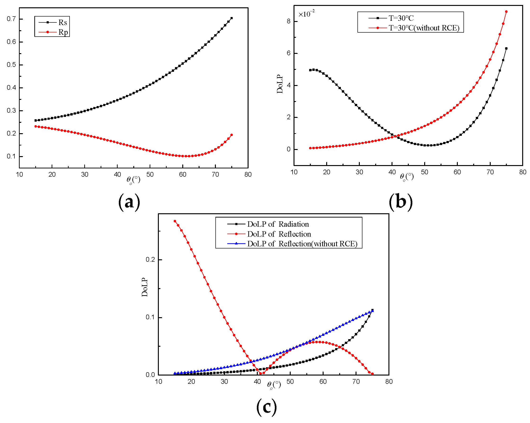
In order to study the influence of RCE on the DoLP, we calculate the Rs, Rp and DoLP of the object according to the proposed model shown in Figure 3, and the object temperature is set at 30 °C in the simulation.

Figure 3a shows that $R_s>R_p$ at all observation angles, so most of the energy of the OTR is concentrated in the p-polarized direction and the Stokes component of the radiated light $S_{OTR,1}$ is less than 0. For natural light incidence, the s-polarized energy of the reflected light is greater than the p-polarized energy; accordingly, the $S_{r,1}$ component of the reflected light is greater than zero. Therefore, the DoLP of the object is related to the ratio of radiation to incident energy. The influence of RCE on the DoLP of the object is shown in Figure 3b. The DoLP of the object increases monotonically with the observation angles without considering RCE. The trend of the DoLP of the object decreases first and then increases while considering RCE, with the minimum value at ${\theta }_O={53}^{\circ }$. In order to analyze the reasons for this influence of RCE, the radiation and reflection DoLP of the object are calculated according to Equations (16) and (19), respectively, as shown in Figure 3c. It can be seen that the DoLP of reflection increases at small observation angles and decreases at lager observation angles due to the influence of RCE. The reason for this is that the RCE changes the incident light from natural light to partial polarization light, thus changing the measurement results of the object’s DoLP. Therefore, RCE must be considered in the study of the polarization characteristics of objects in marine background.

3.1.2. Influence of Object Temperature on the DoLP of Object

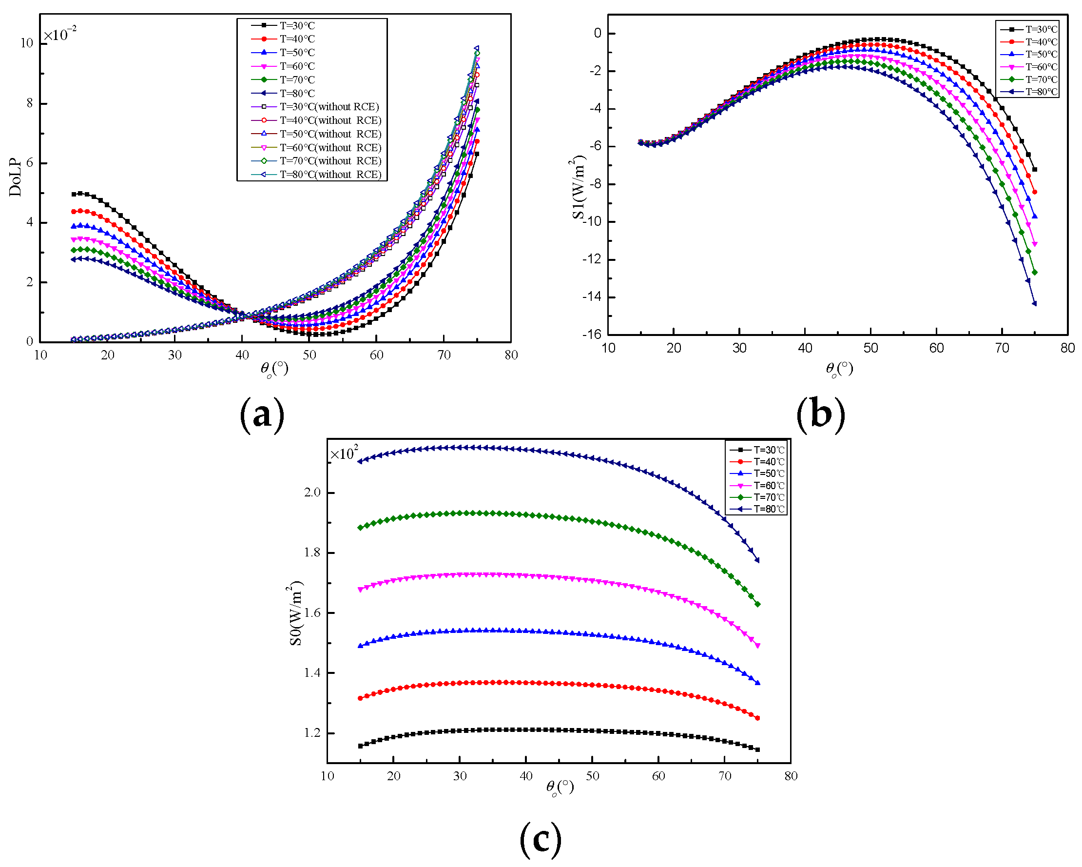
From the above simulation analysis, it can be seen that the object’s temperature changes the ratio of radiated and incident energy, thus changing the DoLP of object. The DoLP of object at different observation angles (15–75°) for object temperatures from 30 °C to 80 °C were calculated, respectively, as shown in Figure 4a.

In comparison with Figure 3b, it can be seen that the trend of DoLP does not change with the object’s temperature. The DoLP of the object decreases with the increase in temperature at small observation angles and increases with the growth of temperature at large observation angles. To explain this result, the $S_0$, $S_1$ components of the Stokes vector at different temperatures are calculated as in Figure 4b,c. At small observation angles, it can be seen that as the object’s temperature increases, the $S_1$ component remains more or less constant, while the $S_0$ component increases significantly. Therefore, in this case, the DoLP of the object decreases with the increase in temperature. At larger observation angles, however, the increase in the object’s temperature will simultaneously increase the $S_0$ and $S_1$ components, but overall, it will cause the DoLP of the object to increase.

3.1.3. Influence of Surface Roughness on the DoLP of Object

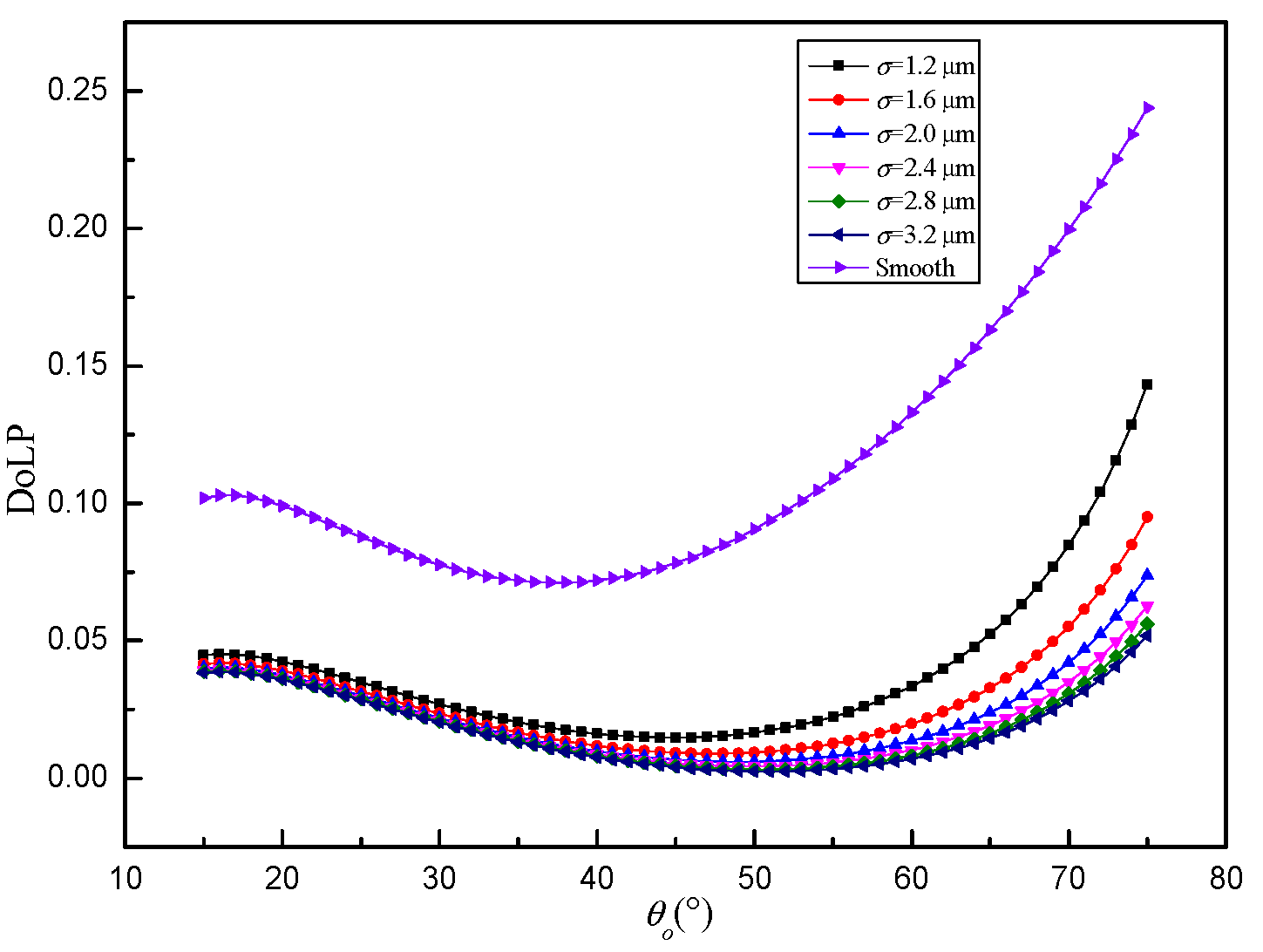
In order to discuss the influence of surface roughness $\sigma$, the object’s DoLP with different $\sigma$ is calculated when the object temperature is 48 ℃, as shown in Figure 5. Compared with Figure 3b, it can be seen that the trend of the object’s DoLP does not change with $\sigma$. The object that has an ideal mirror surface shows the maximum DoLP. With the increase in surface roughness, the DoLP of the object decreases gradually. This is because the rougher the surface is, the smaller the specular reflection component and the larger the diffuse reflection component will be. Therefore, the DoLP of the object will decrease.

3.2. Experimental Verification

3.2.1. The Experimental Setup

To validate the deduced model, an infrared DoLP measurement system is constructed within the wavelength range of 8–14 µm. The object is a painted aluminum plate with a surface roughness of 2.1 µm. The heating plate is fixed behind the object mounted on a turntable, which allows for the adjustment of the object’s temperature and the included angle between the object and the horizontal plane. The turntable is placed inside a container containing sea water. The measured values of complex refractive index of the object and the sea water at the central wavelength are 1.5 + 1.3i and 1.21 + 1.3i, respectively. In the experiments, an LWIR polarization system is used to acquire the object’s images. The resolution of the infrared system is $640\times 512$ pixels and the pixel size is 17 µm. Considering the actual situation, we set the angles between the object and the sea surface within the range of 30–90°, which corresponds to the object observation angles of 15–75°. Sea water temperature is set at 23.5 °C, room temperature 20 °C, relative humidity 72%, and the detector angle is set at α_D = 15°.

3.2.2. Experimental Results

In the experiment, the object is heated to the specified temperature by means of a heating plate. Rotating the polarizing plate at 0°, 45°, 90°, and 135°, the polarization intensity of the object $I_{0^{\circ }}$, $I_{{45}^{\circ }}$, $I_{{90}^{\circ }}$ and $I_{{135}^{\circ }}$ is acquired, respectively. Omitting the circular polarization component, the Stokes vector is obtained as follows,

$$\mathit{S}=\left(\begin{array}{c}{S}_0\\ S_1\\ S_2\\ S_3\end{array}\right)=\left(\begin{array}{c}(I_{0^{\circ }}+I_{{45}^{\circ }}+I_{{90}^{\circ }}+I_{{135}^{\circ }})/2\\ I_{0^{\circ }}-I_{{90}^{\circ }}\\ I_{{45}^{\circ }}-I_{{135}^{\circ }}\\ 0\end{array}\right)$$

Therefore, the DoLP image can be calculated by Equation (9). In the experiment, polarization images are acquired through different observation angles ${\theta }_O$ at object temperatures of 40 °C, 50 °C, and 60 °C, as shown in Figure 6. It can be seen that the DoLP of the object tends to decrease first and then increase with the observation angles, and the minimum value is obtained at ${\theta }_O={55}^{\circ }$. It is basically consistent with the simulation results in Section 3.1. In addition, it can be clearly observed that the DoLP of the object does not tend to zero at small observation angles, which is rightly predicted by the simulation results of the model.

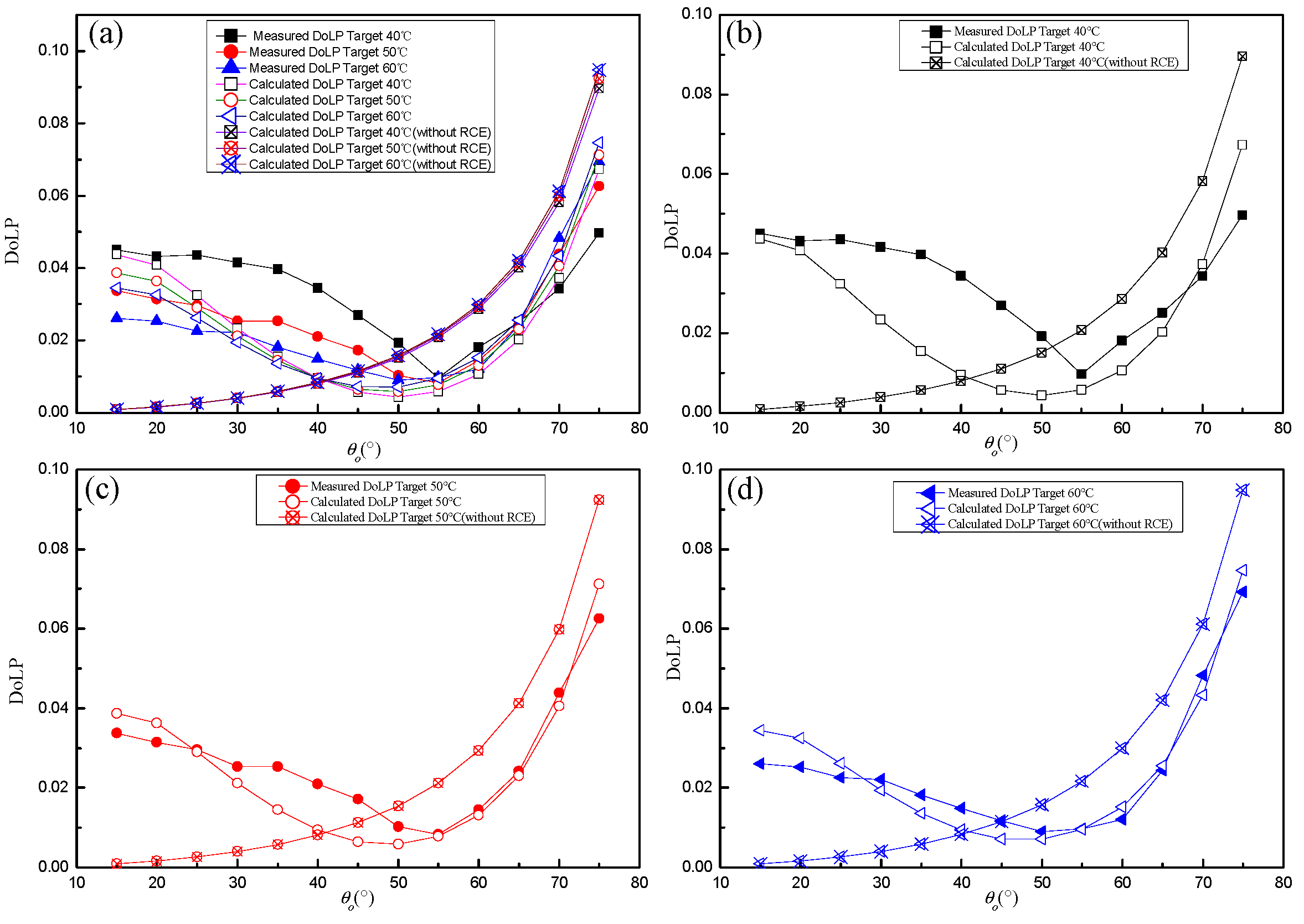
The DoLP of the object is simulated and calculated with and without RCE, respectively. The comparison between the simulation and the experiment is shown in Figure 7. In Figure 7a, it can be seen that the experimental value of the object’s DoLP decreases with increasing temperature for small observation angles, and increases with increasing temperature for large observation angles, which is consistent with the results of the theoretical analysis in Section 3.1.2.

4. Discussion

In the experiment, the minimum value of the object’s DoLP is obtained at an observation angle of 55°, while the minimum value in the simulation results is at the observation angle of 53°, which is mainly caused by the insufficient accuracy of the observation angle interval in the experiment. From Figure 7b–d, it can be seen that the simulation results of the deduced model accord more closely with the experimental results compared to the results without RCE. Overall, the simulation results of the deduced model and experimental results both have the trend of first decreasing and then increasing in terms of the object’s DoLP. The simulation results have smaller minimum and larger maximum values compared with the experimental results, so the simulation results have a larger amplitude than the experimental results, resulting from not taking into account detector errors in the model, such as noise. In addition, it can be found that as the temperature of the object increases, the simulation results are in better agreement with the experimental results, mainly because as the temperature increases, the radiation of the object enhances, while the noise of the detector changes little.

5. Conclusions

In this paper, a DoLP model is deduced for objects in a marine background, taking into account the RCE. The simulation results show a trend of DoLP first decreasing and then increasing, and the minimum DoLP is achieved at ${\theta }_O={53}^{\circ }$. In contrast to the results without RCE, the simulation results of the proposed model have a larger DoLP at small observation angles and a smaller DoLP at large observation angles. The DoLP of the object decreases with increasing temperature at small observation angles and increases with increasing temperature at large observation angles. The DoLP of the object decreases with the increase in roughness, regardless of observation angles.

To verify the simulation results, an LWIR polarization measurement system is constructed, and the DoLP of the object is measured at different temperatures and observation angles. The measured results are consistent with the simulation results. These conclusions are of great significance to the research of polarization detection and identification of infrared objects in the marine background.

References

- Hioki, S.; Riedi, J.; Djellali, M.S. A study of polarimetric error induced by satellite motion: Application to the 3MI and similar sensors. Atmos. Meas. Tech. 2021, 14, 1801–1816. [Google Scholar] [CrossRef]
- Li, S.; Jiao, J.; Wang, C. Research on Polarized Multi-Spectral System and Fusion Algorithm for Remote Sensing of Vegetation Status at Night. Remote Sens 2021, 13, 3510. [Google Scholar] [CrossRef]
- Zhou, Y.; Lu, Y.C.; Shen, Y.F.; Ding, J.; Zhang, M.; Mao, Z. Polarized Remote Inversion of the Refractive Index of Marine Spilled Oil From PARASOL Images Under Sunglint. IEEE Trans. Geosci. Remote Sens. 2020, 58, 2710–2719. [Google Scholar] [CrossRef]
- Yang, M.; Xu, W.; Sun, Z.; Wu, H.; Tian, Y.; Li, L. Mid-wave infrared polarization imaging system for detecting moving scene. Opt. Lett. 2020, 45, 5884–5887. [Google Scholar] [CrossRef] [PubMed]
- Ren, K.; Lv, Y.Y.; Gu, G.H.; Chen, Q. Calculation method of multiangle polarization measurement for oil spill detection. Appl. Opt. 2019, 58, 3317–3324. [Google Scholar] [CrossRef]
- Zhang, J.H.; Zhang, Y.; Shi, Z.G. Enhancement of dim targets in a sea background based on long-wave infrared polarization features. IET Image Process. 2018, 12, 2042–2050. [Google Scholar] [CrossRef]
- Xue, F.D.; Jin, W.Q.; Qiu, S.; Yang, J. Airborne optical polarization imaging for observation of submarine Kelvin wakes on the sea surface: Imaging chain and simulation. ISPRS J. Photogramm. Remote Sens. 2021, 178, 136–154. [Google Scholar] [CrossRef]
- Tyo, J.S.; Ratliff, B.M.; Boger, J.K.; Black, W.T.; Bowers, D.L.; Fetrow, M.P. The effects of thermal equilibrium and contrast in LWIR Polarimetric images. Opt. Express 2007, 15, 15161–15167. [Google Scholar] [CrossRef]
- Felton, M.; Gurton, K.P.; Pezzaniti, J.L.; Chenault, D.B.; Roth, L.E. Measured comparison of the crossover periods for mid- and long-wave IR (MWIR and LWIR) polarimetric and conventional thermal imagery. Opt. Express 2010, 18, 15704–15713. [Google Scholar] [CrossRef] [PubMed]
- Liu, H.Z.; Shi, Z.L.; Feng, B. An Infrared DoLP Computational Model considering Surroundings Irradiance. Infrared Phys. Technol. 2019, 106, 103043. [Google Scholar] [CrossRef]
- Flynn, D.S.; Alexander, C. Polarized surface scattering expressed in terms of a bidirectional reflectance distribution function matrix. Opt. Eng. 1995, 34, 1646–1650. [Google Scholar]
- Priest, R.G.; Germer, T.A. Polarimetric BRDF in the Microfacet Model: Theory and Measurements. In Proceedings of the 2000 Meeting of the Military Sensing Symposia Specialty Group on Passive Sensors, Ann Arbor, MI, USA, 1 May 2000. [Google Scholar]
- Torrance, K.E.; Sparrow, E.M. Theory for off-specular reflection from roughened surfaces. J. Opt. Soc. Am. A 1967, 57, 1105–1114. [Google Scholar] [CrossRef]
- Hyde, M.W.; Schmidt, J.D.; Havrilla, M.J. A geometrical optics polarimetric bidirectional reflectance distribution function for dielectric and metallic surfaces. Opt. Express 2009, 17, 22138–22153. [Google Scholar] [CrossRef]
- Feng, W.W.; Wei, Q.N. A scatterometer for measuring the polarized bidirectional reflectance distribution function of painted surfaces. Infrared Phys. Technol. 2008, 51, 559–563. [Google Scholar]
- Liu, Y.L.; Yu, K.; Liu, Z.L.; Zhao, Y.J.; Liu, Y.F. Polarized BRDF measurement of steel E235B in the near-infrared region: Based on a self-designed instrument with absolute measuring method. Infrared Phys. Technol. 2018, 91, 78–84. [Google Scholar] [CrossRef]
- Jordan, D.L.; Lewis, G. Measurements of the effect of surface roughness on the polarization state of thermally emitted radiation. Opt. Lett. 1994, 19, 692–694. [Google Scholar] [CrossRef] [PubMed]
- Wolff, L.B.; Lundberg, A.; Tang, R. Image understanding from thermal emission polarization. In Proceedings of the 1998 IEEE Computer Society Conference on Computer Vision and Pattern Recognition, Santa Barbara, CA, USA, 25 June 1998. [Google Scholar]
- Gurton, K.P.; Dahmani, R. Effect of surface roughness and complex indices of refraction on polarized thermal emission. Appl. Opt. 2005, 44, 5361–5367. [Google Scholar] [CrossRef] [PubMed]
- Zhang, Y.; Han, J.T.; Li, J.C.; Yang, W.P.; Gong, T. Characteristics analysis of infrared polarization for several typical artificial objects. In Proceedings of the SPIE The International Society for Optical Engineering, Amsterdam, The Netherlands, 23 October 2014. [Google Scholar]
- Liu, F.; Shao, X.P.; Gao, Y.; Li, B.X.; Han, P.L.; Li, G. Polarization characteristics of objects in long-wave infrared range. J. Opt. Soc. Am. A 2016, 33, 237–243. [Google Scholar] [CrossRef]
- Liu, H.; Zhu, J.P.; Wang, K.; Xu, R. Polarized BRDF for coatings based on three-component assumption. Opt. Commun. 2017, 384, 118–124. [Google Scholar] [CrossRef]
- Cheng, Y.Y.; Wang, Y.X.; Niu, Y.Y.; Zhao, Z.R. Concealed object enhancement using multi-polarization information for passive millimeter and terahertz wave security screening. Opt. Express 2020, 28, 6350–6366. [Google Scholar] [CrossRef]
- Zhang, Z.; Wu, Y.; Li, Z. Optical Polarization Characteristics of Low-Earth-Orbit Space Targets. J. Korean Phys. Soc. 2020, 76, 311–317. [Google Scholar] [CrossRef]
- Su, J.L.; Wu, H.F.; Li, P.F.; Hu, Y.; Hu, F. Detection for ship by dual-polarization imaging radiometer. Opt. Express 2021, 29, 27830–27844. [Google Scholar] [CrossRef]
- Tuo, H.N.; Shi, G.C.; Luo, X.L. Detection Method of Ship Target Infrared Polarization Image. In Proceedings of the 7th International Conference on Computer-Aided Design, Manufacturing, Modeling and Simulation (CDMMS 2020), Busan, Korea, 14–15 November 2020. [Google Scholar]
- Zhang, X.F.; Nie, X.F.; Du, Z.Q. Target polarization characteristics analysis and detection in complex background. In Proceedings of the 2021 International Conference on Electrical, Electronics and Computing Technology (EECT 2021), Xiamen, China, 26–28 March 2021. [Google Scholar]
- Wei, M.; Zhang, Y.; Shi, Z.G.; Zhang, Y.; Liu, P.J. Analysis of visible/infrared polarization characteristics of small UAV with complex background of buildings. In Proceedings of the Third International Conference on Image, Video Processing and Artificial Intelligence, Shanghai, China, 21–23 August 2020. [Google Scholar]
- Zhang, J.H.; Zhang, Y.; Shi, Z.G. Study and modeling of infrared polarization characteristics based on sea scene in long wave band. J. Infrared Millim. Waves 2018, 37, 586–594. [Google Scholar]
- Gil, J.J.; Ossikovski, R. Polarized Light and the Mueller Matrix Approach, 1st ed.; CRC Press: Boca Raton, FL, USA, 2016; pp. 107–109. [Google Scholar]
- Thilak, V.; Voelz, D.G.; Creusere, C.D. Polarization-based index of refraction and reflection angle estimation for remote sensing applications. Appl. Opt. 2007, 46, 7527–7536. [Google Scholar] [CrossRef] [Green Version]
- Resnick, A.; Persons, C.; Lindquist, G. Polarized emissivity and Kirchhoff’s law. Appl. Opt. 1999, 38, 1384–1387. [Google Scholar] [CrossRef]
Figure 1.
The model of infrared radiation in marine background. and are the observation angle and the incidence angle, respectively; is the angle between the object and the sea surface.
Figure 2.
Geometry relation of micro-surface model.
Figure 3.
Influence of RCE on the DoLP of object: (a) Reflectance of the s-polarized and p-polarized components; (b) the DoLP of the object; and (c) the DoLP of reflection and radiation.