Article

Analysis of Error Sources in the Lissajous Scanning Trajectory Based on Two-Dimensional MEMS Mirrors

1
School of Automation Science and Electrical Engineering, Beihang University, Beijing 100191, China
2
School of Instrumentation and Optoelectronic Engineering, Beihang University, Beijing 100191, China
3
College of Future Technology, Peking University, Beijing 100871, China
4
Beijing Transcend Vivoscope Biotech Co., Ltd., Beijing 100049, China
5
State Key Laboratory of Advanced Optical Communication System and Networks, School of Electronics, Peking University, Beijing 100871, China
6
Key Laboratory of Precision Opto-Mechatronics Technology (Ministry of Education), Beihang University, Beijing 100191, China
7
Laboratory of Intelligent Sensing Materials and Chip Integration Technology of Zhejiang Province, Hangzhou Innovation Institute of Beihang University, Hangzhou 310063, China
*
Authors to whom correspondence should be addressed.
Photonics 2023, 10(10), 1123; https://doi.org/10.3390/photonics10101123
Submission received: 26 June 2023 / Revised: 25 September 2023 / Accepted: 4 October 2023 / Published: 6 October 2023
(This article belongs to the Section Biophotonics and Biomedical Optics)

Abstract

:
Deviations or distortions in the trajectoy of MEMS-based Lissajous scanning imaging platforms might be detrimental to imaging quality. These deviations often arise from differences in MEMS mirror frequency response characteristics and asymmetry in parameters within the measurement and control circuit. This study concentrated on the measurement and control circuit unit as it identified and analyzed four error sources: the MEMS mirror frequency response error, the AD acquisition synchronization error, the drive source error, and the cross-coupling error between the MEMS mirror axes. This study constructed a Lissajous trajectory test platform based on oscilloscopes and a position sensitive detector. Consequently, its experimental results guided the error processing methods to access the feasibility of the compensation methods by combining measured trajectories. Overall, regarding MEMS-based Lissajous scanning platforms for biomedical imaging, this study could provide quantitative numerical references for error analysis, image reconstruction, and aberration correction.

1. Introduction

The MEMS mirror, employing Micro-Electro-Mechanical Systems (MEMS) and beam control technologies, offers advantages such as rapid response, compact size, and relatively wide scanning angles [1,2]. Two-dimensional MEMS mirrors have extensive applications in portable and miniature microscopic imaging instruments, including confocal microscopy [3,4,5], nonlinear microscopy [6,7,8,9,10], and photoacoustic microscopy [11,12,13]. They come in various types, driven by different mechanisms like electrostatic, electromagnetic, thermoelectric, and piezoelectric methods [1]. Among these, electrostatic MEMS mirrors offer the advantage of a relatively higher scanning frequency to enable faster frame rates. Researchers have explored various scanning schemes, including raster scanning, spiral scanning, and Lissajous scanning [14]. Lissajous scanning, in particular, offers light uniformity, trajectory parameter selection flexibility, and robust adaptability [15,16].
Several research groups have explored MEMS-based Lissajous scanning techniques for confocal and two-photon microscopy. Previous work primarily focused on aspects like the frequency selection principle of the Lissajous patterns, the design and optimization of MEMS mirrors, enhancements to optical and mechanical probe schemes, as well as hardware and software techniques to improve image quality [17,18,19,20]. However, limited research has focused on characterizing the control circuitry within Lissajous imaging systems, specifically in indentifying the error sources. The complex control circuit, coupled with several error factors, can introduce deviations or distortions into Lissajous trajectories, posing challenges for image reconstruction and imaging quality degradation. Moreover, closed-loop control strategies for integrated portable/miniature confocal and two-photon microscopy systems remain a persistent challenge when relying on feedback from sensing elements. Alternatively, open-loop feedforward control strategies are typically employed, which necessitate prior knowledge of quantitative error data. This information proves crucial for fine-tuning control circuitry drive signal parameters during feedforward compensation control and determining key parameters, such as the amplitude and phase for image reconstruction. Consequently, investigating error sources within the measurement and control circuitry holds theoretical and practical importance in advancing MEMS-based biomedical platforms.
In this work, we performed an analysis of error sources in the Lissajous scanning trajectory based on two-dimensional MEMS mirrors. The theory of Lissajous graphs and signal parameters that define the Lissajous trajectory were introduced, providing a theoretical basis for subsequent error analysis and compensation. Furthermore, we identified four error sources within the measurement and control circuit unit: the MEMS mirror frequency response error, the AD acquisition synchronization error, the drive source error, and the cross-coupling error between MEMS mirror axes. We designed and implemented a test platform using oscilloscopes and a position sensitive detector (PSD). For each type of error source, experimental methods were developed to quantitatively determine the errors. Finally, error calibration experiments were conducted, to verify the existence of error types, assess their magnitudes, and demonstrate the feasibility of error compensation. This work could provide quantitative references for the implementation of error analysis, image reconstruction, and aberration correction in MEMS-based Lissajous scanning microscopy.

2. Methods

2.1. Lissajous Theory

The Lissajous trajectory represents the compounded path followed by a point undergoing harmonic motion along both x and y axes [21]. Its mathematical description can be expressed by Equation (1).
x = A x sin 2 π f x t + φ x y = A y sin 2 π f y t + φ y .
A x and A y are the amplitudes of the x and y axes, f x and f y are the frequencies of the x and y axes, and φ x and φ y are the initial phases of the x and y axes.
Applying the inverse sine function to both sides of Equations (1) and (2) is calculated as follows:
2 π f x t + φ x + 2 i π = ± sin 1 x A x 2 π f y t + φ y + 2 j π = ± sin 1 y A y ,
where i , j are arbitrary integers. By performing calculations on Equation (2), Equation (3) is obtained as follows:
f x f y = φ x 2 i π ± sin 1 x A x φ y 2 j π ± sin 1 y A y .
The frequency ratio parameters m = f x g c d f x , f y and n = f y g c d f x , f y are defined, with g c d f x , f y being the maximum common divisor of f x and f y . Taking m n = f x f y (where m , n are mutually prime integers) into Equation (3), Equation (4) is deduced as follows:
m φ y n φ x + 2 ( j m i n ) π = ± m sin 1 y A y n sin 1 x A x .
By taking the sine of both sides of Equation (4), Equation (5) is presented as follows:
sin m φ y n φ x = sin m sin 1 y A y ± n sin 1 x A x .
From the trajectory equation presented in Equation (5), the Lissajous trajectory is evidently determined by the frequency ratio parameters m , n and m φ y n φ x [22] when the values of amplitudes A x and A y are fixed. The trajectory refresh frequency (frame rate) of the Lissajous scanning trajectory corresponds to the maximum common divisor of f x and f y .

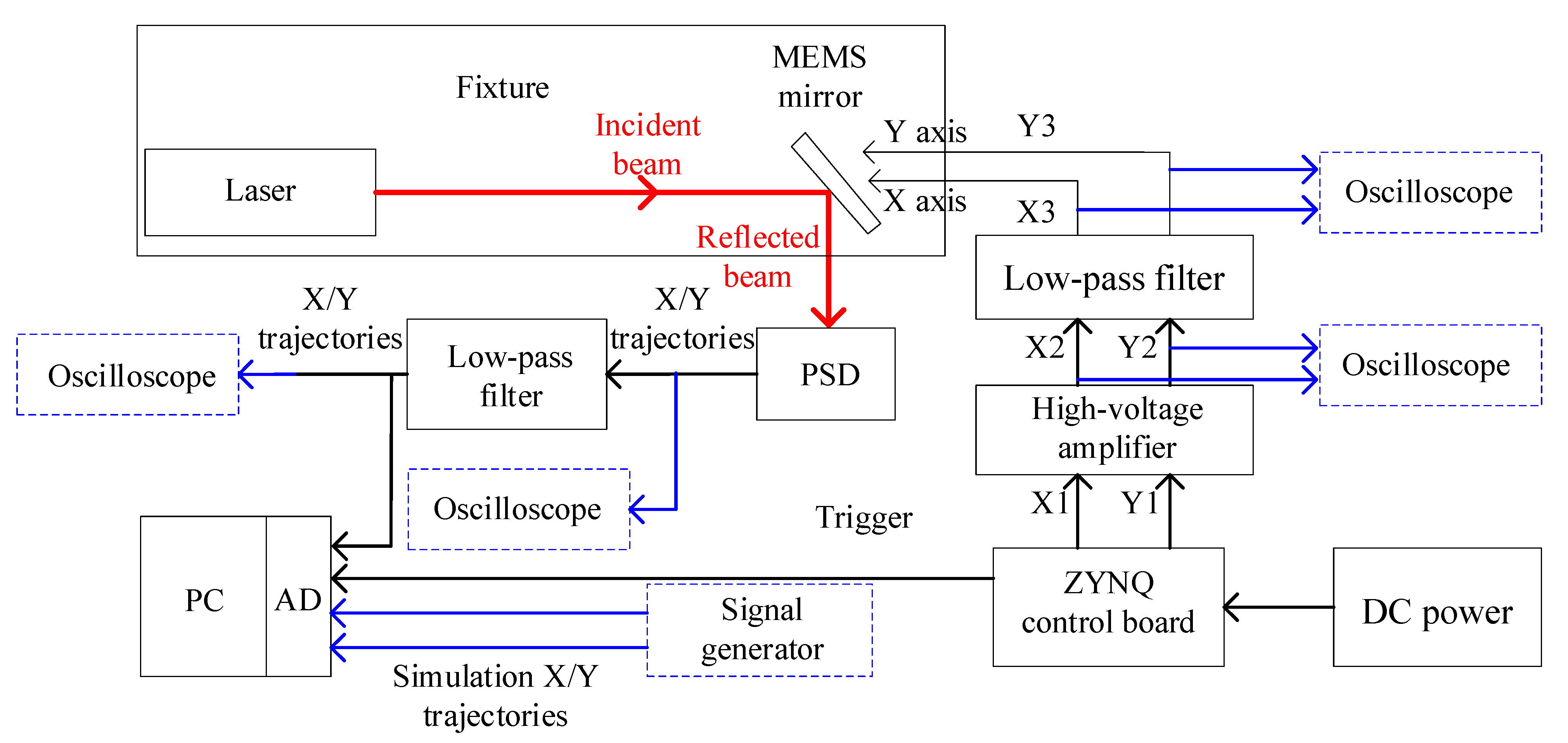
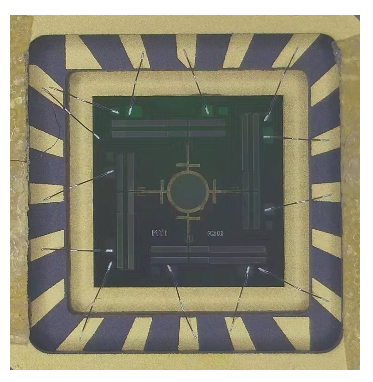
2.2. MEMS Scanning Lissajous Trajectory Test Platform Overview

To investigate error factors within the MEMS-based Lissajous scanning system, a test platform was constructed as illustrated in Figure 1. The platform mainly consisted of a customized ZYNQ control board, a high-voltage amplification circuit, a low-pass filtering circuit, a MEMS mirror, a laser, a PSD, an analog-to-digital module (AD), a personal computer (PC), and oscilloscopes.
The ZYNQ control board was used to generate the differential signals for driving the MEMS mirror, with a phase difference of ±180°. These signals offered programmable control over their frequency (range from 0 to 10 kHz), amplitude (range from 0 V to +10 V), and phase (range from 0° to 360°). The high-voltage amplification circuit generated a high-voltage differential driving signal with a DC bias of 80 V and a peak-to-peak voltage ranging from −150 V to +150 V. The signal contained high-frequency noise, which was filtered out by the low-pass filtering circuit with a cutoff frequency of 20 kHz before being utilized to drive the MEMS mirror.
The laser (M-16A650-10, Hengjiu LED, Guangzhou, China) operated at a wavelength of 650 nm, delivered 10 mW of power, and featured an adjustable output spot diameter. The fixtures were used to position the laser and the MEMS mirror, ensuring that the laser beam was incident onto the center of MEMS mirror surface at a 45° angle with slightly shifts in the incident point position within ±4° range. During scanning, the reflected beam was incident on the PSD, which converted the light trajectory into electrical signals. After being processed by the filtering circuit, these signals could be either visualized on an oscilloscope to observe the scanning trajectory or collected by the AD module and subsequently uploaded to the PC. The digital oscilloscope (TDS2012C, Tektronix, Beaverton, OR, USA) boasted a bandwidth of 100 MHz and a sampling rate of 2 GS/s. Given that the signal frequencies did not exceed 5 kHz, the presence of the oscilloscope had a negligible impact on the measurement and control circuitry. In YT mode and XY mode, the single and combined electrical characteristics could be observed, respectively.
For the AD acquisition module, the PXI card (PXI3223) was employed, featuring eight parallel acquisition channels, 14-bit acquisition precision, adjustable sampling rates ranging from 1 to 20 MSa/s, and a measurement range of ±10 V. The PC was a chassis-controller configuration manufactured by National Instruments. The PSD (PDP90A, Thorlabs, Newton, NJ, USA) was selected for its 15 kHz bandwidth, a typical output signal amplitude accuracy of 0.3 mV, and a detection area of up to 9 mm × 9 mm.

3. Experimental Validation

In the experimental validation, we focused on four error sources in MEMS-based Lissajous scanning platforms: the MEMS mirror frequency response error, the AD acquisition synchronization error, driver source errors, and the cross-coupling error between MEMS mirror axes. These error sources were analyzed and tested, as described in Section 3.1, Section 3.2, Section 3.3 and Section 3.4.

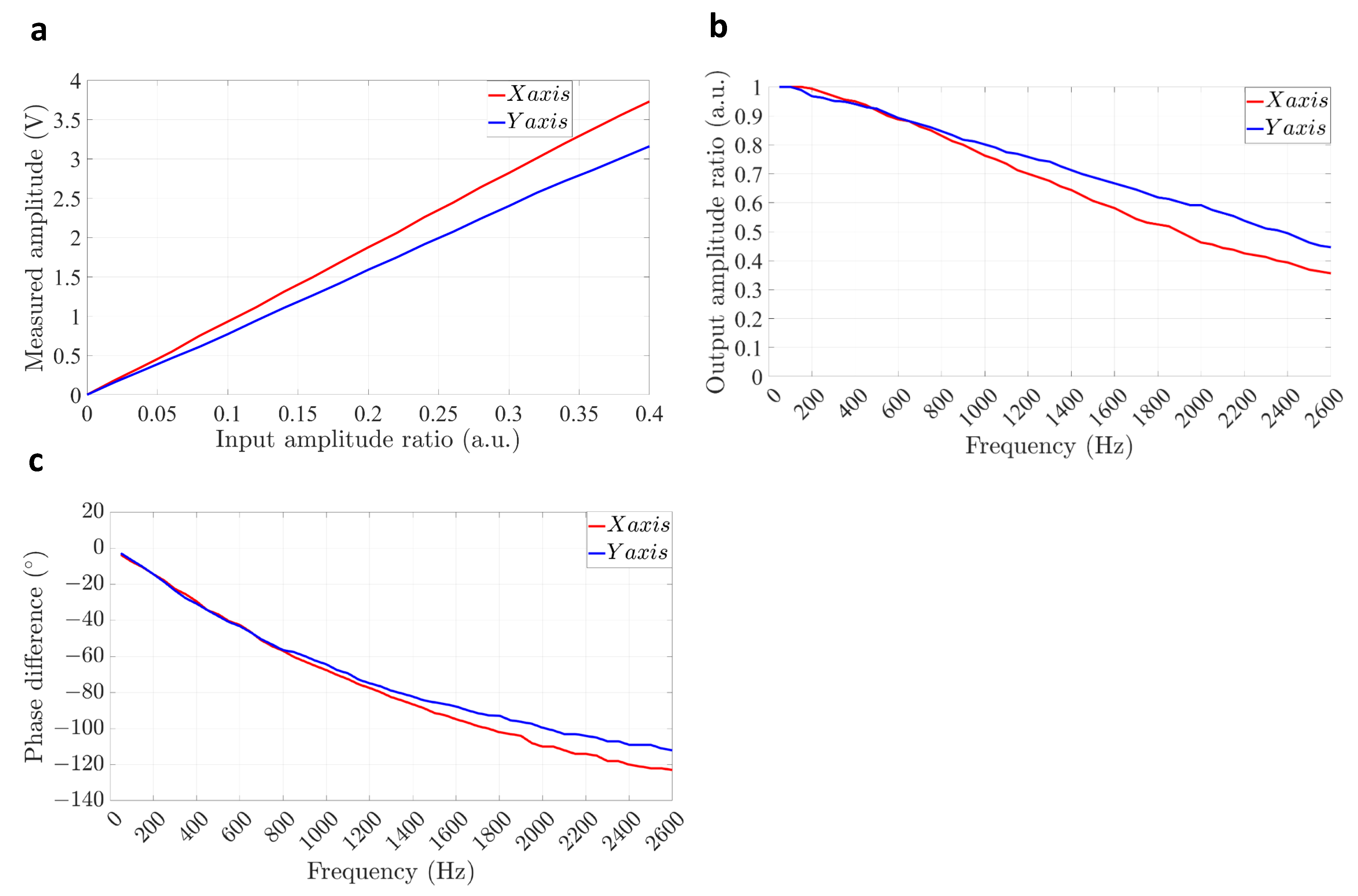
3.1. Frequency Response Error of a Two-Dimensional MEMS Mirror

A two-dimensional quasi-static MEMS mirror (A3I12.2, Mirrorcle Technologies, Richmond, CA, USA) was selected for the Lissajous scanning platform [23], as depicted in Figure 2. This aluminum-coated scanning mirror operated with a differential drive on both of its axes, featuring a mirror diameter of 1.2 mm, a maximum differential voltage of 150 V, and a single-ended signal DC bias of 80 V. The mechanical deflection angle of the mirror had a range of up to ±5.4°, with resonant frequencies of 2937 Hz for the X axis and 2913 Hz for the Y axis. This mirror exhibited operational capability across the frequency range from zero to its resonant frequencies, thereby offering flexible frequency selectivity for Lissajous trajectory [24].
To investigate the influence of frequency characteristics on the trajectory of the MEMS mirror, we designed a model for its frequency response test, as depicted in Figure 3 [25]. The control circuit generated two-channel high-voltage differential signals with a DC bias of 80 V and a phase difference of π , which drove both the X and Y axes of the MEMS mirror. The signals induced mechanical angular vibrations of the mirror, resulting in the generation of a Lissajous trajectory [26]. A PSD was employed to convert the light signal into electrical signals along both axes [27]. Oscilloscopes were used to measure the amplitude and phase information of the Lissajous trajectory. Given the sufficiently high bandwidth of the PSD and the oscilloscopes compared to the MEMS mirror, the obtained results reflected the operational characteristics of the MEMS mirror.
To account for the MEMS’s mirror lifespan and practicality, this study limited the operating frequency to 2600 Hz. The output amplitudes of the measurement and control circuit (also the input amplitude of the MEMS mirror), denoted as V x , and V y , were restricted to 40% of the full-scale range V m a x . Employing the model presented in Figure 3, we conducted frequency response tests for both axes of the MEMS mirror. The measured output amplitudes of the PSD signals were recorded as V x , and V y . The measured phase differences between the input MEMS drive signals and PSD output signals were measured as φ x = Θ x Φ x , and φ y = Θ y Φ y . At a specific frequency of 50 Hz, the measured output amplitudes of the PSD signals were recorded as V x 0 and V y 0 . The measured amplitude of the PSD signals versus the input amplitude ratio curves is depicted in Figure 4a. Based on this figure, when the input amplitude ratio was set as 0.2, the measured amplitudes were noted as V x 0 , and V y 0 . The amplitude frequency response curves obtained in this situation are depicted in Figure 4b. In this figure, the horizontal axis represents the frequency, and the vertical axis represents the output amplitude ratios of two axes, V x V x 0 and V y V y 0 . Meanwhile, the phase frequency response curves obtained in this situation are depicted in Figure 4c. The horizontal axis represents the frequency, and the vertical axis represents the phase differences of two axes, φ x and φ y . The variations in the MEMS mirrors’ X and Y axes, in conjunction with their associated DA circuits, high-voltage amplification circuits, and low-pass filtering circuits, led to differences in the frequency response characteristics. The experimental results indicated that when the frequency was below 800 Hz, the frequency response characteristics of both axes closely matched. However, within the frequency range of 800 Hz to 2600 Hz, the amplitude ratio of the X axis exceeded that of the Y axis by less than 0.1. The phase difference of the X axis exceeded that of the Y axis, with a difference within a range of 10°.
Furthermore, we selected specific drive signal parameters as follows: f x = 2300   H z , f x = 2300   H z , V x = V y = 0.2   V m a x , and Φ x = Φ y = 0 ° . By referring to Figure 4, we derived the actual scanning trajectory for the X axis, which had an amplitude of V x = 0.51   V x 0 = 1.91   V and a phase of Θ x = 107 ° , and for the Y axis, which had an amplitude of V y = 0.45   V y 0 = 1.43   V and a phase of Θ x = 112 ° . Note that the amplitudes and phases of the two axes were not equal. This quantitative information can be used to compensate for the frequency response error caused by the MEMS mirror.

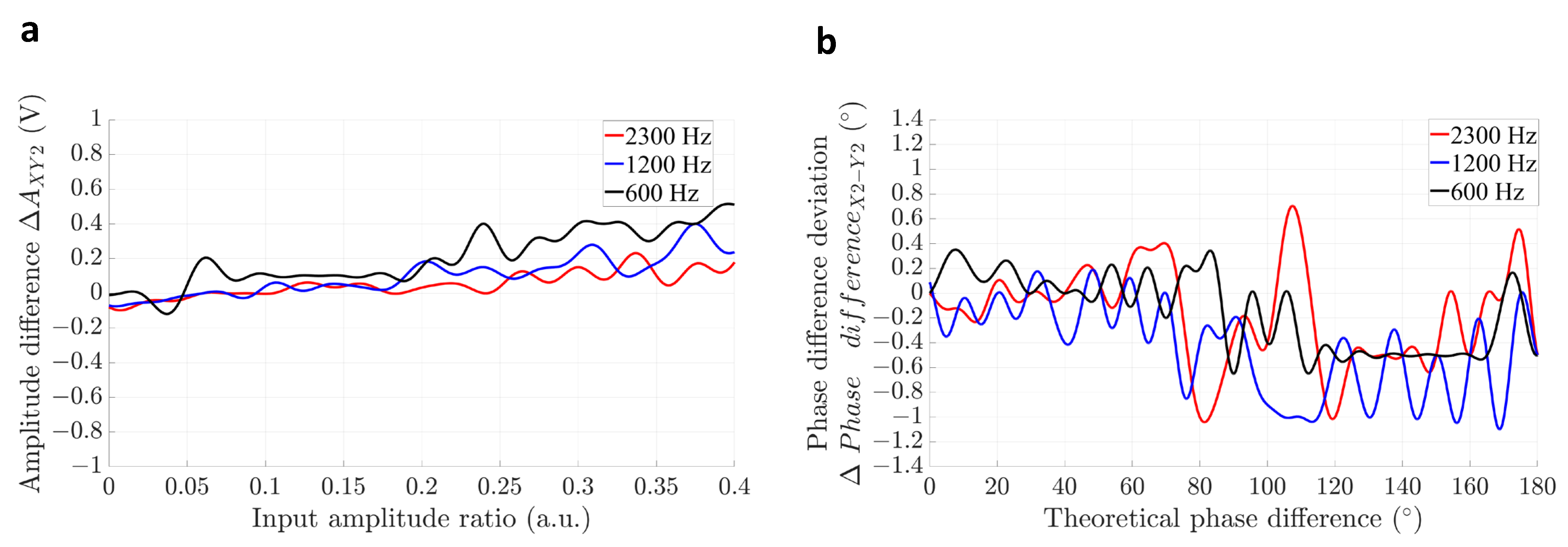
3.2. AD Acquisition Synchronization Error

The AD circuit mainly comprises a conditioning circuit and an AD integrated chip. In cases involving multiple AD acquisition channels, differences in phase frequency characteristics arise due to the asymmetry of circuit parameters among the channels. When the frequency of the acquired signal varies across these channels, it exacerbates phase delays. Consequently, the initially set phase difference for the acquired signal deviates from its theoretical value, resulting in an AD acquisition synchronization error.
As per Lissajous graph theory, variations in phase between X and Y axes lead to alterations in the Lissajous trajectory [28]. To illustrate this point, we considered two sets of parameters, V x = V x = 5   V , V y = V y = 5   V , f x = f x = 1200   H z , and f y = f y = 1300   H z , differing only in the initial phase φ x = φ x = 0 ° , φ y = 0 ° , φ y = 1 ° . Two theoretical Lissajous trajectories were plotted, as illustrated in Figure 5a,b. After zooming in Figure 5a, a deviation between the two theoretical trajectories became noticeable, as depicted in Figure 5b. This trajectory deviation could induce distortion during image reconstruction.
A signal generator was used to generate two sine signals for the X and Y channels, with the following parameters: V x = 5   V , f x = 1200   H z , φ x = 0 ° and V y = 5   V , f y = 1300   H z , φ y = 0 ° . Subsequently, two independent parallel AD channels simultaneously captured the X and Y signals at a sampling rate set of 10M Sa/s, The overview and zoomed-in view of the uncompensated measured Lissajous trajectory, along with the theoretical trajectory 1, were plotted, respectively, as shown in Figure 6a,b. The synchronization between the acquisition of the two AD channels deviated, leading to a change in the initial phase difference between the X and Y signals and causing an offset in the Lissajous trajectory. The uncompensated measured trajectory partially coincided with the theoretical trajectory 1.
Furthermore, the initial phase of the X axis φ x remained unaltered, and the initial phase of the Y axis φ y was adjusted. When the compensated measured trajectory coincided with the theoretical trajectory 1, the initial phase of the Y axis, φ y = 1.12 ° , corresponding to a phase adjustment, φ y = φ y φ y = 1.12 ° . φ y could be regarded as the AD acquisition synchronization error under the specified parameters. As depicted in Figure 6c,d, we observed an improved overlap between the compensated measured Lissajous trajectory and the theoretical trajectory 1. Note that the phase adjustment values were determined for specific frequency parameters. When the frequencies of the X and Y axes signals changed, the phase adjustment values also altered accordingly.

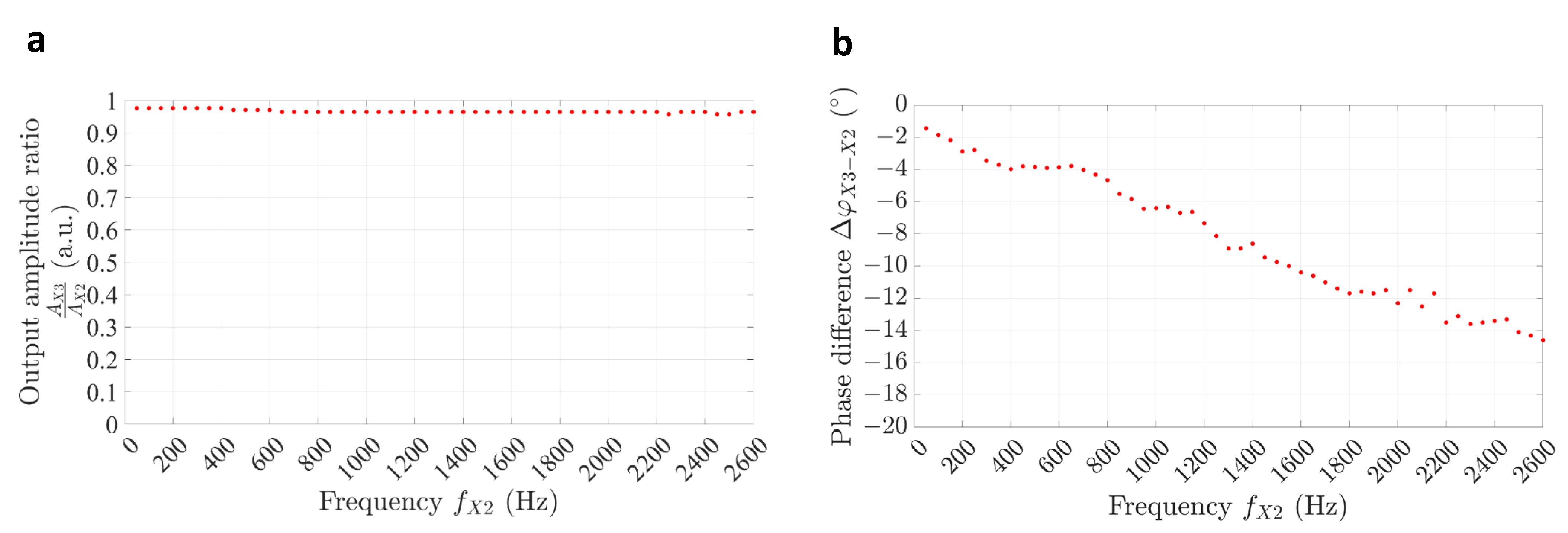
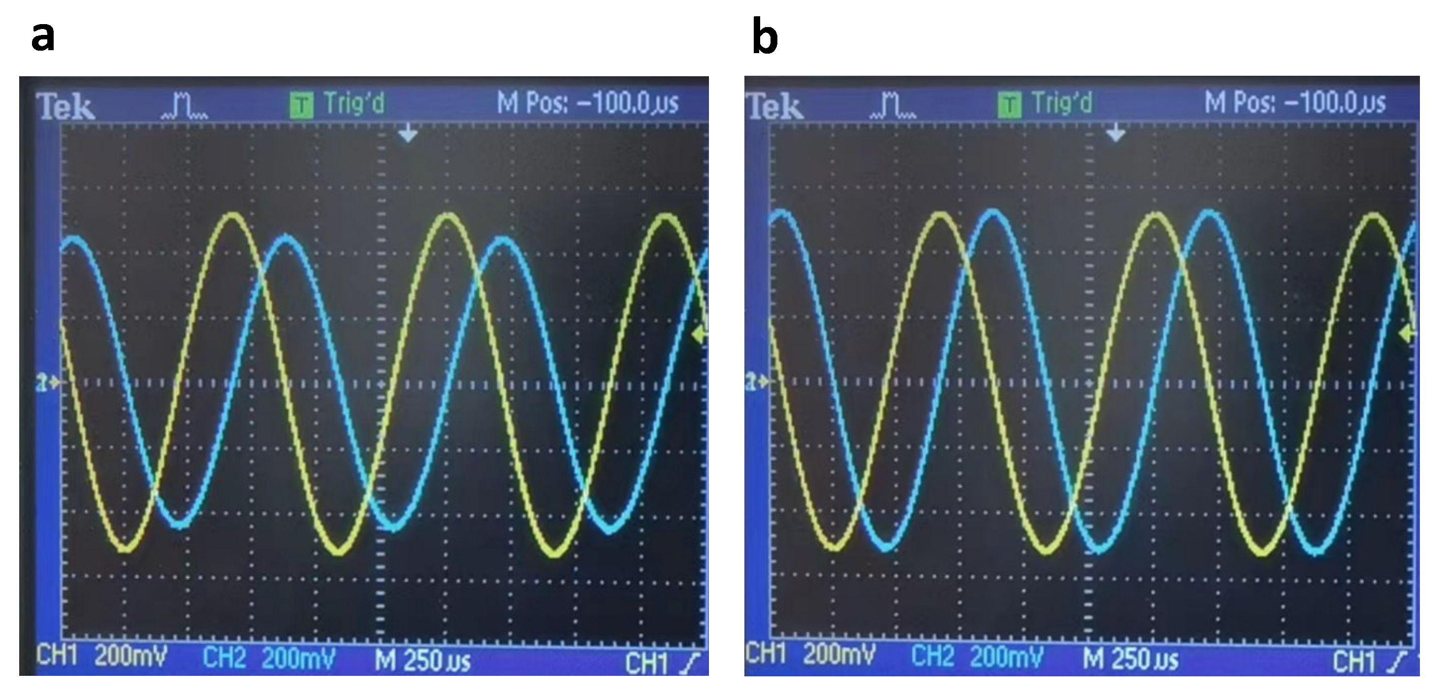
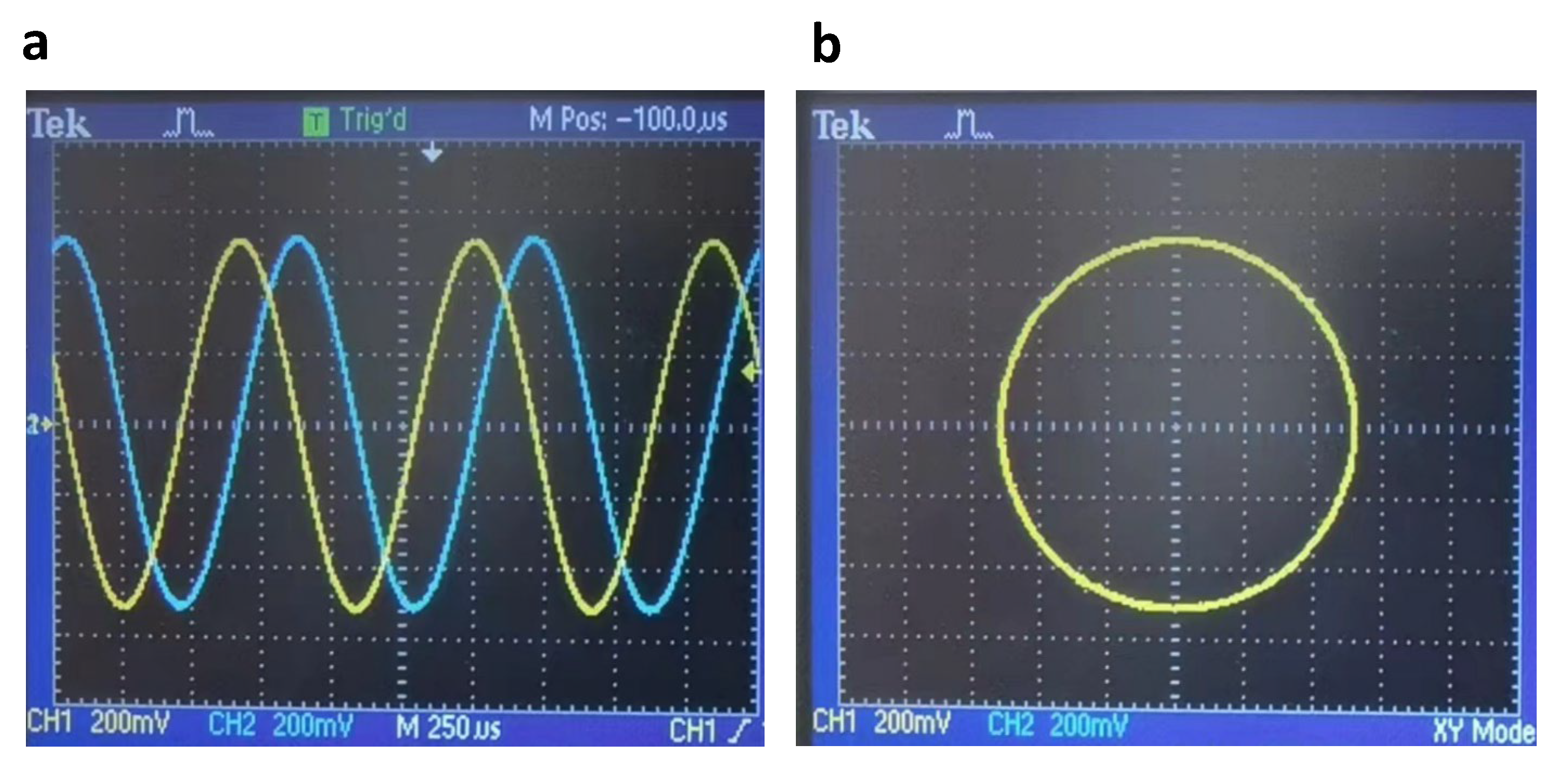
3.3. Drive Source Error

Within the platform, the measurement and control unit generated the drive signals for the MEMS mirror, consisting of the voltage generation circuit, the bias conditioning circuit, the high-voltage amplifier circuit, and the low-pass filter circuit [29,30,31,32]. Due to asymmetry in the circuit parameters and frequency characteristics, the measured drive signals deviated from the theoretical signals, particularly in the amplitude and phase. These discrepancies in drive source resulted in a mismatch between the theoretical and measured trajectories [33].
By referring to Figure 1a, we used an oscilloscope to monitor the drive signals output by the high-voltage amplifier circuit at three frequencies: 2300 Hz, 1200 Hz, and 600 Hz. We quantified the measured amplitude differences and deviations in the phase differences between X2 and Y2 relative to their input signals, denoted as A X 2 Y 2 and P h a s e   d i f f e r e n c e X 2 Y 2 , respectively. As depicted in Figure 7a, the amplitude difference A X 2 Y 2 exhibited an overall increasing trend, fluctuating within the range of −0.1 V to +0.9 V. Furthermore, as presented in Figure 7b, the deviations in phase differences P h a s e   d i f f e r e n c e X 2 Y 2 ranged from −1° to +0.6°.
To assess the impact of the low-pass filter circuit on the drive source error, we performed tests on the X3 channels. The frequency response curves of the low-pass filter circuit are illustrated in Figure 8a,b. The input amplitude V X 2 = 0.2   V m a x , φ X 2 = 0 ° . The results indicated that the measured output amplitude ratio A X 3 A X 2 consistently exceeded 0.97, and the measured phase difference φ X 3 X 2 varied between −1° and −15°.
To establish a reference for the Lissajous trajectory, the drive signal parameters were set as follows: V X = 0.2   V m a x , V Y = 0.2 V m a x , f X = 2300 H z , f Y = 1200 H z , f X f Y = m n = 23 12 , φ X = 0 ° , φ Y = 0 ° , and m φ Y n φ X = 0 ° and were generated by the signal generator. The reference Lissajous trajectory was observed by an oscilloscope, as illustrated in Figure 9a,b.
The parameters were also set and output by the measurement and control circuit for testing the Lissajous trajectory. Figure 9c,d display the uncompensated Lissajous trajectory, exhibiting a reduction in the X axis amplitude. The measured amplitudes for X3 and Y3 axes were 13.3 V and 15.72 V, and the amplitude difference A X 3 Y 3 was approximately −2.4 V, and the phase difference φ X 3 Y 3 was approximately −6.3°. The calculated m φ Y n φ X 0 ° , which resulted in a deviation from the reference Lissajous trajectory. Figure 9e,f show the compensated Lissajous trajectory. The X axis amplitude increased by 2.4 V, such that the amplitude difference A X 3 Y 3 = 0 V. The Y axis phase remained unchanged, while the X axis phase adjusted by φ X = 6.3 ° , such that m φ Y n φ X + φ X = 0 ° . These results indicated that the compensated Lissajous trajectory aligned with the reference Lissajous trajectory.

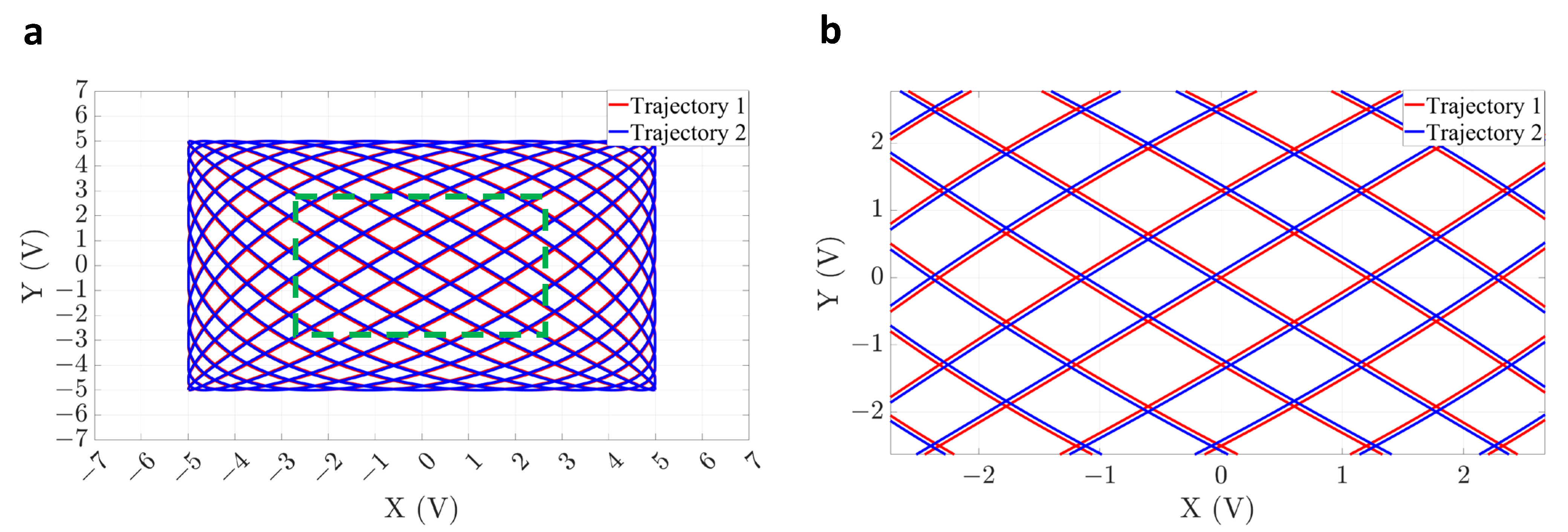
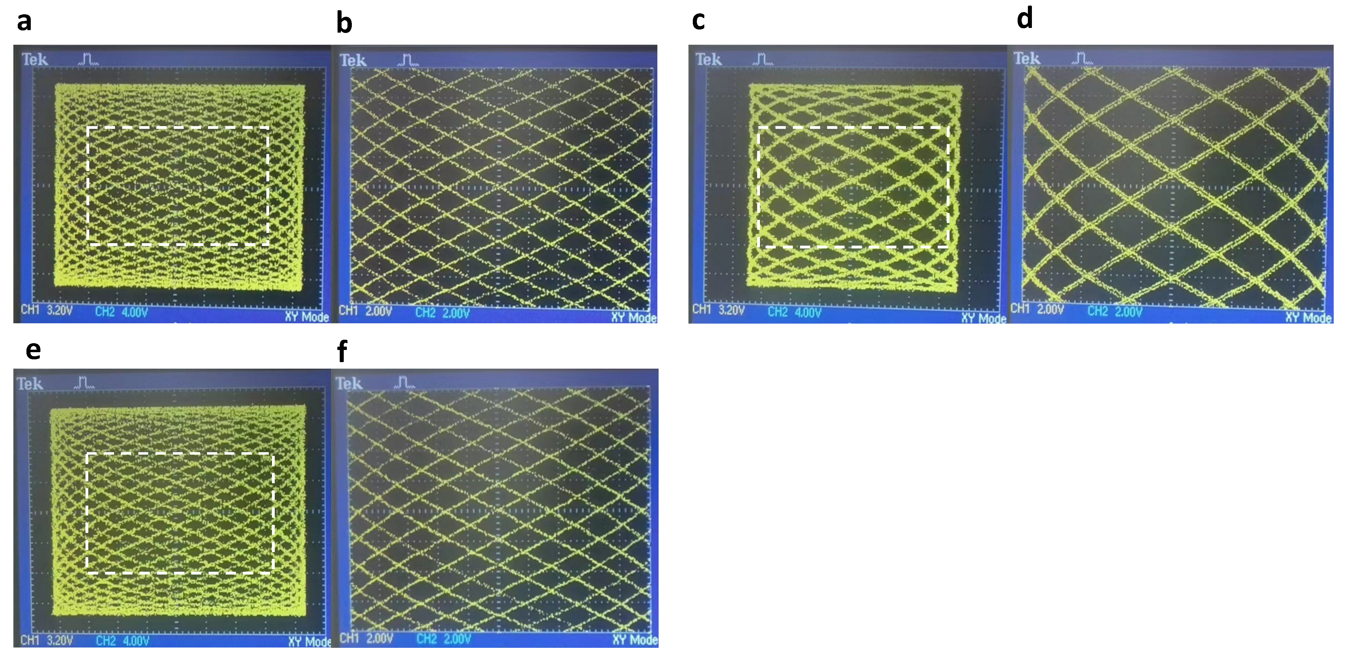
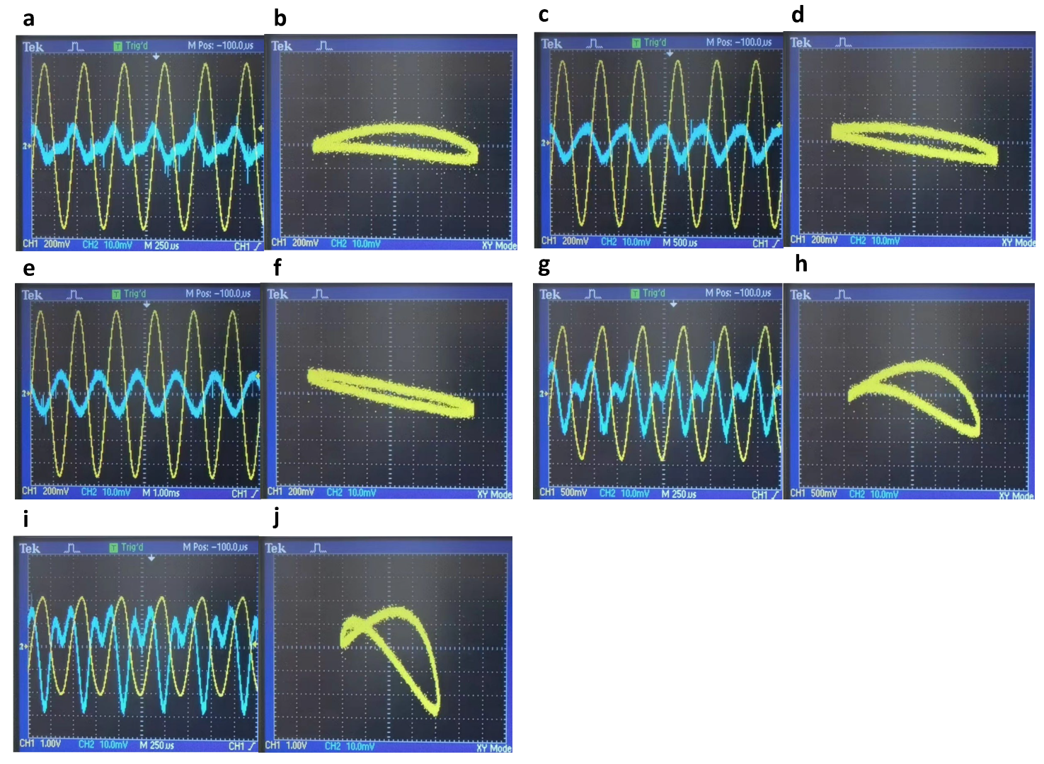
3.4. Cross-Coupling Error between the MEMS Mirror Axes

The two-dimensional MEMS mirror utilizes biaxial mechanical vibration to precisely control the reflector’s position. It employs a double-axis orthogonal support beam structure. As such, machining process errors, including support beam width, unequal elasticity, and mass asymmetry, can lead to inter-axis cross-coupling interference [34,35,36]. In [37], the presence of asymmetry along both axes, resulted in unequal elasticity, leading to the generation of coupling forces. The Equation describing the coupling force along the Y axis is as follows:
F y = sin 2 α 2 ( k x x k y y ) x ,
where α represents the angle between the elastic and inertial principal axis, k x x and k y y are the stiffness coefficients along the X and Y axes, respectively, and variable ‘x’ denotes the displacement of the X axis support beam. The coupling force along the Y axis induces the deflection of its support beams around the X axis, subsequently driving the scanning mirror’s deflection and generating a trajectory component in the Y axis.
Given the symmetry and similarities between the MEMS mirror’s X and Y axes, we conducted the test on the X axis. Five sets of sinusoidal signals with different amplitudes V X and frequencies f X were applied to the X axis, while the amplitude of Y axis was set to zero. PSD was used to capture the trajectory of the MEMS mirror and convert it into electrical signals. The specific parameters of the X and Y signals were observed in the YT mode of the oscilloscope, and the trajectory was observed in the XY mode, as illustrated in Figure 10. In the first set of waveforms (a), (b), and (c), the amplitude was fixed at V X = 0.1   V m a x and the frequencies were set to 2300 Hz, 1200 Hz, and 600 Hz, respectively. In the second set of waveforms (a), (d), and (e), the frequency was fixed at f X = 2300   H z , and the amplitudes V X were set to 0.1   V m a x , 0.2   V m a x , and 0.3   V m a x , respectively.
As depicted in Figure 10a–c, when the amplitude was fixed at V X = 0.1   V m a x , the trajectory captured in the oscilloscope’s YT Mode exhibited a component in the Y direction [38], with respective amplitudes of 8.8 mV, 9.8 mV, and 10.4 mV. These frequencies aligned with the X axis operating frequency, and the coupling error amplitude tended to decrease as the signal frequency increased. These variations in coupling interference amplitude were attributed to the amplitude frequency characteristics of the MEMS mirror, as discussed in Section 3.1. Specifically, the MEMS mirror exhibited low-pass characteristics, causing an increased amplitude attenuation and a decrease in the oscillation angle along the X axis with higher frequencies. Consequently, this attenuation weakened the coupling forces acting on the Y axis, resulting in reduced interference in the Y axis deflection. This reduction was manifested as a decrease in the amplitude component along the Y axis, consistent with experimental results.
As depicted in Figure 10a,d,e, when the frequency was fixed at f X = 2300   H z , there was a component in the Y direction, with respective amplitudes of 8.8 mV, 15.6 mV, and 22.6 mV. The coupling error amplitude tended to increase as the driving signal amplitude increased and the MEMS mirror vibration amplitude increased. As the amplitude of the MEMS mirror’s X axis vibration increased, the amplitude of coupling errors in the Y axis also rose. This increase in coupling interference aligned with the experimental observations as the X axis amplitude continued to increase. The single axis cross-coupling error characteristics presented above revealed an inter-axis coupling interference phenomenon when the MEMS mirror was in operation. The coupling error was found dependent on the driving signal parameters, with a signal-to-noise ratio of approximately 40 dB.
In practical Lissajous scanning situation, effective drive signals were applied to both MEMS mirror axes. For example, a group of input drive signals paramters were considered: V X = V Y = 0.1   V m a x , f X = f Y = 1200   H z , and φ X = 0 ° ,   φ Y = 90 ° . As depicted in Figure 11a,b, the Y axis peak-to-peak signals were compensated by +0.4 V, while the X and Y axes’ phase difference was compensated by +0.2°, effectively eliminating the drive source signal error (Section 3.3). Furthermore, by referring to Section 3.4, the Y axis peak-to-peak signals were compensated by +0.16 V, while the X and Y axes phase difference was compensated by −2.6°, as shown in Figure 12a,b, thus eliminating the effect of the MEMS mirror frequency response characteristics. The compensated waveforms and combined trajectory were then obtained, as shown in Figure 13a,b. The theoretical trajectory, representing a circle, closely matched the measured trajectory after eliminating the source signal and MEMS mirror frequency response errors. Additionally, the cross-coupling error (less than 20 mV) exhibited a minimal impact in the practical two-dimensional scanning applications.

4. Conclusions

This study aimed to analyze the error sources in MEMS-based Lissajous scanning platforms. To provide a theoretical foundation for error analysis and compensation, we introduced Lissajous graph theory and essential signal parameters. Furthermore, we identified four error sources within the measurement and control circuit and developed dedicated experimental methods for quantitative assessment. Finally, error calibration experiments were conducted, to verify the existence of error types, assess their magnitudes, and demonstrate the feasibility of error compensation. Overall, this study offers essential quantitative error references for implementing feedforward control and image reconstruction in MEMS-based Lissajous scanning microscopy.
In forthcoming research endeavors, we aspire to further develop Lissajous scanning miniature nonlinear microscopy using two-dimensional MEMS mirrors. In this case, our upcoming research focus will prioritize high-density scans of Lissajous trajectories, precise circuit synchronization, thus achieving the integration of miniature nonlinear probes for biomedical applications, including label-free endomicroscopic imaging and brain imaging in freely behaving mice.

Author Contributions

Conceptualization, X.Z. and L.F.; methodology, X.Z., C.W., Y.H. (Yongxuan Han), J.W. (Junjie Wang), Y.H. (Yanhui Hu), J.W. (Jie Wang) and Q.F.; Validation, X.Z., C.W. and Y.H. (Yongxuan Han); software, X.Z., Y.H. (Yongxuan Han), Y.H. (Yanhui Hu) and J.W. (Jie Wang); writing—original draft preparation, X.Z. and Y.H. (Yongxuan Han); writing—review and editing, X.Z., C.W., Y.H. (Yongxuan Han), A.W., L.F. and X.H.; supervision, A.W., L.F. and X.H.; project administration, A.W., L.F. and X.H.; funding acquisition, A.W., L.F. and X.H. All authors have read and agreed to the published version of the manuscript.

Funding

This work was supported by the National Key Research and Development Program of China (2020YFB1312802), National Natural Science Foundation of China (61973019, 31830036, and 61975002), and the Academic Excellence Foundation of BUAA for PhD students.

Institutional Review Board Statement

Not applicable.

Informed Consent Statement

Not applicable.

Data Availability Statement

Not applicable.

Conflicts of Interest

The authors declare no conflict of interest.

References

  1. Holmström, S.T.S.; Baran, U.; Urey, H. MEMS laser scanners: A review. J. Microelectromech. Syst. 2014, 23, 259–275. [Google Scholar] [CrossRef]
  2. Fujita, T.; Maenaka, K.; Takayama, Y. Dual-axis MEMS mirror for large deflection-angle using SU-8 soft torsion beam. Sens. Actuators. A. 2005, 121, 16–21. [Google Scholar] [CrossRef]
  3. Piyawattanametha, W.; Wang, T.D. MEMS-based dual-axes confocal microendoscopy. IEEE J. Sel. Top. Quantum Electron. 2009, 16, 804–814. [Google Scholar] [CrossRef] [PubMed]
  4. Jeon, J.; Kim, H.; Jang, H.; Hwang, K.; Kim, K.; Park, Y.G.; Jeong, K.H. Handheld laser scanning microscope catheter for real-time and in vivo confocal microscopy using a high definition high frame rate Lissajous MEMS mirror. Biomed. Opt. Express 2022, 13, 1497–1505. [Google Scholar] [CrossRef]
  5. Pan, T.; Gao, X.; Yang, H.; Cao, Y.; Zhao, H.; Chen, Q.; Xie, H. A MEMS mirror-based confocal laser endomicroscope with image distortion correction. IEEE Photonics J. 2023, 15, 3900408. [Google Scholar] [CrossRef]
  6. Tang, S.; Jung, W.; McCormick, D.; Xie, T.; Su, J.; Ahn, Y.C.; Tromberg, B.J.; Chen, Z. Design and implementation of fiber-based multiphoton endoscopy with microelectromechanical systems scanning. J. Biomed. Opt. 2009, 14, 034005. [Google Scholar] [CrossRef]
  7. Murugkar, S.; Smith, B.; Srivastava, P.; Moica, A.; Naji, M.; Brideau, C.; Stys, P.K.; Anis, H. Miniaturized multimodal CARS microscope based on MEMS scanning and a single laser source. Opt. Express 2010, 18, 23796–23804. [Google Scholar] [CrossRef]
  8. Duan, X.; Li, H.; Qiu, Z.; Joshi, B.P.; Pant, A.; Smith, A.; Kurabayashi, K.; Oldham, K.R.; Wang, T.D. MEMS-based multiphoton endomicroscope for repetitive imaging of mouse colon. Biomed. Opt. Express 2015, 6, 3074–3083. [Google Scholar] [CrossRef] [PubMed]
  9. Klioutchnikov, A.; Wallace, D.J.; Frosz, M.H.; Zeltner, R.; Sawinski, J.; Pawlak, V.; Voit, K.M.; Russell, P.S.J.; Kerr, J.N.D. Three-photon head-mounted microscope for imaging deep cortical layers in freely moving rats. Nat. Methods 2020, 17, 509–513. [Google Scholar] [CrossRef]
  10. Zong, W.; Wu, R.; Chen, S.; Wu, J.; Wang, H.; Zhao, Z.; Chen, G.; Tu, R.; Wu, D.; Hu, Y.; et al. Miniature two-photon microscopy for enlarged field-of-view, multi-plane and long-term brain imaging. Nat. Methods 2021, 18, 46–49. [Google Scholar] [CrossRef]
  11. Guo, H.; Song, C.; Xie, H.; Xi, L. Photoacoustic endomicroscopy based on a MEMS scanning mirror. Opt. Lett. 2017, 42, 4615–4618. [Google Scholar] [CrossRef]
  12. Lee, C.; Kim, J.Y.; Kim, C. Recent progress on photoacoustic imaging enhanced with microelectromechanical systems (MEMS) technologies. Micromachines 2018, 9, 584. [Google Scholar] [CrossRef]
  13. Li, L.; Liang, X.; Qin, W.; Guo, H.; Qi, W.; Jin, T.; Tang, J.; Xi, L. Double spiral resonant MEMS scanning for ultra-high-speed miniaturized optical microscopy. Optica 2023, 10, 1195–1202. [Google Scholar] [CrossRef]
  14. Hwang, K.; Seo, Y.H.; Jeong, K.H. Microscanners for optical endomicroscopic applications. Micro Nano Syst. Lett. 2017, 5, 1. [Google Scholar] [CrossRef]
  15. Liang, W.; Murari, K.; Zhang, Y.; Chen, Y.; Li, M.J.; Li, X. Increased illumination uniformity and reduced photodamage offered by the Lissajous scanning in fiber-optic two-photon endomicroscopy. J. Biomed. Opt. 2012, 17, 021108. [Google Scholar] [CrossRef]
  16. Kim, D.Y.; Hwang, K.; Ahn, J.; Seo, Y.H.; Kim, J.B.; Lee, S.; Yoon, J.H.; Kong, E.; Jeong, Y.; Jon, S.; et al. Lissajous scanning two-photon endomicroscope for in vivo tissue imaging. Sci. Rep. 2019, 9, 3560. [Google Scholar] [CrossRef]
  17. Du, W.; Zhang, G.; Ye, L. Image quality analysis and optical performance requirement for micromirror-based Lissajous scanning displays. Sensors 2016, 16, 675. [Google Scholar] [CrossRef]
  18. Seo, Y.H.; Hwang, K.; Kim, H.; Jeong, K.H. Scanning MEMS mirror for high definition and high frame rate Lissajous patterns. Micromachines 2019, 10, 67. [Google Scholar] [CrossRef]
  19. Wang, J.; Zhang, G.; You, Z. Design rules for dense and rapid Lissajous scanning. Microsyst. Nanoeng. 2020, 6, 101. [Google Scholar] [CrossRef]
  20. Zhang, Y.; Liu, Y.; Wang, L.; Su, Y.; Zhang, Y.; Yu, Z.; Zhu, W.; Wang, Y.; Wu, Z. Resolution adjustable Lissajous scanning with piezoelectric MEMS mirrors. Opt. Express 2023, 31, 2846–2859. [Google Scholar] [CrossRef]
  21. Xu, D.; Zhang, F. Parameters of Lissajous graphs. J. Qufu Norm. Univ. 2001, 27, 54–56. [Google Scholar]
  22. Zhang, X. Analysis of influence of initial phase on Lissajous graph. J. Hubei Normal. Univ. 2000, 20, 56–60. [Google Scholar]
  23. Wong, L.; Yie, J.; Park, S. Selective Infiltration Damping of MEMS Scanning Mirrors. In Proceedings of the 2018 International Conference on Optical MEMS and Nanophotonics (OMN), Lausanne, Switzerland, 29 July–2 August 2018; pp. 1–2. [Google Scholar]
  24. Wong, L.; Yie, J.; Park, S. Convex optimization on differential pair of actuation voltages for quasi-Static MEMS Mirrors in scanning applications. In Proceedings of the 22nd International Conference on Control, Automation and Systems, Jeju, Republic of Korea, 27 November–1 December 2022; pp. 592–596. [Google Scholar]
  25. Tanguy, Q.A.A.; Gaiffe, O.; Passilly, N.; Cote, J.M.; Cabodevila, G.; Bargiel, S.; Lutz, P.; Xie, H.; Gorecki, C. Real-time Lissajous imaging with a low-voltage 2-axis MEMS scanner based on electrothermal actuation. Opt. Express. 2020, 28, 8512–8527. [Google Scholar] [CrossRef]
  26. Birla, M.; Duan, X.; Li, H.; Lee, M.; Li, G.; Wang, T.; Oldham, K.R. Image processing metrics for phase identification of a multiaxis MEMS scanner used in single pixel imaging. IEEE-ASME Trans. Mechatron. 2021, 26, 1445–1454. [Google Scholar] [CrossRef]
  27. Chen, H.; Sun, Z.; Sun, W.; Yeow, J.T.W. Twisting sliding mode control of an electro-static MEMS micromirror for a laser scanning system. IEEE/CAA J. Autom. Sinica. 2019, 6, 1060–1067. [Google Scholar] [CrossRef]
  28. Han, X. Study on the Features of Lissajous’ Figure. J. XinZhou Teach. Univ. 2009, 25, 18–22. [Google Scholar]
  29. Pologruto, T.A.; Sabatini, B.L.; Svoboda, K. ScanImage: Flexible software for operating laser scanning microscopes. BioMed. Eng. OnLine 2003, 2, 13. [Google Scholar] [CrossRef]
  30. Frigerio, P.; Molinari, L.; Barbieri, A.; Zamprogno, M.; Mendicino, G.; Boni, N.; Langfelder, G. Nested closed-Loop control of Quasi-Static MEMS scanners with large dynamic range. IEEE Trans. Ind. Electron. 2022, 70, 4217–4225. [Google Scholar] [CrossRef]
  31. Wang, J.; Li, H.; Tian, G.; Deng, Y.; Liu, Q.; Fu, L. Near-infrared probe-based confocal microendoscope for deep-tissue imaging. Biomed. Opt. Express 2018, 9, 5011–5025. [Google Scholar] [CrossRef]
  32. Schelinski, U.; Knobbe, J.; Dallmann, H.G.; Grüger, H.; Förster, M.; Scholles, M.; Schwarzenberg, M.; Rieske, R. MEMS Based Laser Scanning Microscope for Endoscopic Use; MOEMS and Miniaturized Systems X; SPIE: San Francisco, CA, USA, 2011; Volume 7930, pp. 23–32. [Google Scholar]
  33. Li, G.; Duan, X.; Lee, M.; Birla, M.; Chen, J.; Oldham, K.R.; Wang, T.D.; Li, H. Ultra-Compact microsystems-based confocal endomicroscope. IEEE Trans. Med. Imaging. 2017, 36, 1482–1490. [Google Scholar] [CrossRef]
  34. Tatar, E.; Alper, S.E.; Akin, T. Effect of quadrature error on the performance of a fully-decoupled MEMS gyroscope. In Proceedings of the 24th International Conference on Micro Electro Mechanical Systems (MEMS), Cancun, Mexico, 23–27 January 2011; pp. 569–572. [Google Scholar]
  35. Weinberg, M.S.; Kourepenis, A. Error sources in in-plane silicon tuning-fork MEMS gyroscopes. J. Microelectromech. Syst. 2006, 15, 479–491. [Google Scholar] [CrossRef]
  36. Yang, B.; Wang, S.; Li, H.; Huang, L.; Li, K.; Yin, Y. The coupling error analysis of the decoupled silicon micro-gyroscope. In Proceedings of the 5th IEEE International Conference on Nano/Micro Engineered and Molecular Systems, Xiamen, China, 20–23 January 2010; pp. 356–361. [Google Scholar]
  37. Shi, Q.; Qiu, A.; Su, Y.; Zhu, X. Mechanical coupling error of silicon microgyroscope. Opt. Precis. Eng. 2008, 16, 894–898. [Google Scholar]
  38. Weinstein, D.; Bhave, S.A.; Tada, M.; Mitarai, S.; Ikeda, K. Mechanical coupling of 2D resonator arrays for MEMS filter applications. In Proceedings of the IEEE International Frequency Control Symposium Joint with the 21st European Frequency and Time Forum, Geneva, Switzerland, 29 May–1 June 2007; pp. 1362–1365. [Google Scholar]
Figure 1. The schematic diagram of the MEMS-based Lissajous trajectory test platform. PSD: position sensitive detector. AD: analog-to-digital module. PC: personal computer. DC power: direct current power. Red arrows indicate the optical path. Blue arrows signify the signal paths generated by the signal generator and observed by the oscilloscope. Finally, the black arrows represent the signal paths generated by the ZYNQ control board and the X/Y trajectory paths.
Photonics 10 01123 g001
Figure 2. A photograph of a two-dimensional MEMS mirror.
Photonics 10 01123 g002
Figure 3. The MEMS mirror frequency response test model.
Photonics 10 01123 g003
Figure 4. The MEMS mirror frequency response characteristics. Red line: X axis. Blue line: Y axis. (a) Measured amplitude of the PSD output signals versus the input amplitude ratio curves. The input amplitude ratio varied from 0 to 0.4. (b) Amplitude frequency response curves. The frequency varied from 50 Hz to 2600 Hz in 50-Hz increments. The input amplitude ratio was set as 0.2. (c) Phase frequency response curves. The frequency varied from 50 Hz to 2600 Hz in 50 Hz increments. The input amplitude ratio was set as 0.2.
Photonics 10 01123 g004
Figure 5. Overall and zoomed-in diagrams of two theoretical Lissajous trajectories. (a) Overall view. (b) Zoomed-in view of the green dashed box labeled in (a).
Photonics 10 01123 g005
Figure 6. Overall and zoomed-in diagrams of the measured and theoretical trajectories. (a) Overall view of the uncompensated measured and theoretical trajectory 1. (b) Zoomed-in view of the green dashed box labeled in (a). (c) Overall view of the compensated measured and theoretical trajectory 1. (d) Zoomed-in view of the green dashed box labeled in (c).
Photonics 10 01123 g006
Figure 7. The characteristics of the drive source errors at three different frequencies. (a) Amplitude difference A X 2 Y 2 versus the input amplitude ratio curves. The input amplitude V X 2 = V Y 2 . (b) Phase difference deviation P h a s e   d i f f e r e n c e X 2 Y 2 versus input phase difference curves. The input amplitude V X 2 = V Y 2 = 0.2   V m a x .
Photonics 10 01123 g007
Figure 8. Low-pass filter circuit frequency response characteristics. Frequency f X 2 vary from 50 Hz to 2600 Hz in 50 Hz increments. (a) Amplitude frequency response curve. (b) Phase frequency response curve.
Photonics 10 01123 g008
Figure 9. The overall and zoomed-in diagrams of the Lissajous trajectories. (a) The reference Lissajous trajectory. (b) The zoomed-in view of the white box in (a). (c) The uncompensated measured Lissajous trajectory. (d) The zoomed-in view of the white box in (c). (e) The compensated measured Lissajous trajectory. (f) The zoomed-in view of the white box in (e).
Photonics 10 01123 g009
Figure 10. Cross-coupling error characteristics of the MEMS mirror’s X axis. Yellow line: X axis. Blue line: Y axis. They indicate the results of the PSD waveform signals from the X and Y axes captured in the oscilloscope’s YT mode at different drive conditions. (a,b V X = 0.1   V m a x , f X = 2300   H z . (c,d) V X = 0.1   V m a x , f X = 1200   H z . (e,f) V X = 0.1   V m a x , f X = 600   H z . (g,h) V X = 0.2   V m a x , f X = 2300   H z . (i,j) V X = 0.3   V m a x , f X = 2300   H z .
Photonics 10 01123 g010
Figure 11. Source drive signal waveforms captured in the YT mode. Yellow line: X axis. Blue line: Y axis. (a) Uncompensated X and Y axis waveforms. V X = 13.6   V , V Y = 14   V , f X = f Y = 1200   H z . X and Y axes’ phase difference of 89.8°. (b) Compensated X and Y axis waveforms. V X = 14   V , V Y = 14   V , f X = f Y = 1200   H z . X and Y axes’ phase difference of 90°.
Photonics 10 01123 g011
Figure 12. Signal waveforms after eliminating the effect of MEMS mirror frequency response characteristics captured in the YT mode. Yellow line: X axis. Blue line: Y axis. (a) Uncompensated X and Y axis waveforms. V X = 0.88   V , V Y = 1.04   V , f X = f Y = 1200   H z . X and Y axes’ phase difference 92.6°. (b) Compensated X and Y axis waveforms. V X = 0.88   V , V Y = 1.04   V , f X = f Y = 1200   H z . X and Y axes’ phase difference 90°.
Photonics 10 01123 g012
Figure 13. Compensated trajectory waveforms. Yellow line: X axis. Blue line: Y axis. (a) X and Y axis waveforms in the YT mode. V X = V Y = 1.04   V , f X = f Y = 1200   H z . X and Y axes’ phase difference 90°. (b) Combined trajectory in the XY mode.
Photonics 10 01123 g013
Disclaimer/Publisher’s Note: The statements, opinions and data contained in all publications are solely those of the individual author(s) and contributor(s) and not of MDPI and/or the editor(s). MDPI and/or the editor(s) disclaim responsibility for any injury to people or property resulting from any ideas, methods, instructions or products referred to in the content.

