Comparison between the Propagation Properties of Bessel–Gauss and Generalized Laguerre–Gauss Beams


1
Molecular Horizons, School of Chemistry and Molecular Biology, University of Wollongong, Wollongong, NSW 2522, Australia
2
Nanoscopy and NIC@IIT, Istituto Italiano di Tecnologia, Via Enrico Melen, 83 Edificio B, 16152 Genova, Italy
3
Complex Systems Group, ETSIME, Universidad Politécnica de Madrid, Ríos Rosas 21, 28003 Madrid, Spain
*
Author to whom correspondence should be addressed.
Photonics 2023, 10(9), 1011; https://doi.org/10.3390/photonics10091011
Submission received: 4 August 2023
/
Revised: 24 August 2023
/
Accepted: 29 August 2023
/
Published: 4 September 2023
Abstract
:The connections between Laguerre–Gauss and Bessel–Gauss beams, and between Hermite–Gauss and cosine-Gauss beams are investigated. We review different asymptotic expressions for generalized Laguerre and Hermite polynomials of large radial/transverse order. The amplitude variations of generalized Laguerre–Gauss beams, including standard and elegant Laguerre–Gauss beams as special cases, are compared with Bessel–Gauss beams. Bessel–Gauss beams can be well-approximated by elegant Laguerre–Gauss beams. For non-integral values of the Laguerre function radial order, a generalized Laguerre–Gauss beam with integer order matches the width of the central lobe well, even for low radial orders. Previous approximations are found to be inaccurate for large azimuthal mode number (topolgical charge), and an improved approximation for this case is also introduced.
1. Introduction
In three dimensions (3D), Laguerre–Gauss [1] (LG) and Bessel–Gauss [2,3] (BG) beam modes are perhaps the most important analytically-expressed beams that propagate paraxially in free space. They are solutions of the paraxial, scalar wave equation (Schrödinger equation). In these types of beam, the field in a cross-section is given by the product of a Laguerre polynomial or a Bessel function, respectively, with a Gaussian. The BG beam is an approximation to the (nonphysical) Bessel beam, which exhibits a propagational invariance (often called a ‘non-diffracting’ or ‘diffraction-free’) property and reconstructs (more correctly, is regenerated) upon propagation through a scattering medium [2,4]. For a non-zero azimuthal mode number (topological charge), LG and BG beams result in helical modes, and exhibit a vortex phase singularity that carries orbital angular momentum [5,6]. In 2D, there are analogous Hermite–Gauss [1] (HG) and cosine-Gauss (cG) beams [7]. The 2D forms can be used to represent field variations in the x and y directions in Cartesian coordinates in 3D space. Relationships and transformations between LG and HG modes were given by Abramochkin, and by Kimel and Elias [8,9].
Applications of these beams are extensive, and range from optical propagation, Fresnel reflection and transmission coefficients, laser resonators, beam waveguides, optical waveguides, optical trapping and manipulation, optical angular momentum, high capacity optical communications using mode multiplexing, imaging, depth of focus extension, optical alignment, optical metrology, nonlinear optics, laser material processing, through to quantum optics, quantum cryptography and quantum computing. Here, we investigate the connection between LG and BG beams, or HG and cG beams, but concentrate specifically on the cylindrical, LG/BG, case.
For the standard HG beam (sHG), the scaling between the two functions is of the form , where n is the mode number, while for the standard LG beam (sLG), it is of the form , where are the radial and azimuthal mode numbers, respectively. Siegman introduced the so-called elegant Hermite–Gauss (eHG) beam, where the relevant scaling of the functions is different, , from the standard sHG beams [10]. There are also elegant Laguerre–Gauss (eLG) beams, [11,12,13]. The elegant beams provide important connections with multipole radiation and spherical harmonics, and with differential operators [11,14,15]. The standard sHG, sLG beams propagate with a transverse amplitude given by a polynomial that does not change in shape, but the amplitude of the elegant beams is described by a polynomial that is a function of a complex parameter, and the shape does change with propagation. Wünsche, and also Pratesi and Ronchi, showed that other, complex, scalings produce a range of propagation effects [12,16,17]. We have called these generalized (gHG, gLG) beams [18].
Turning now to the Bessel beam, an infinitely narrow annular pupil was known to give a Bessel function amplitude point spread function by Rayleigh [19]. (Actually, Airy earlier derived the power series expansion for the Bessel beam, but before the terminology of Bessel functions was universally recognized [20].) The increase in the depth of focus attainable using a narrow annular exit pupil was perhaps first explicitly reported by Steward in 1926 [21]:
{‘… it is evident that the distance between successive dark points upon the axis … tends to infinity as [the normalized radius of the obscuration] tends to unity, as, indeed, is obvious from the consideration that in the limiting case the aperture reduces to a circular rim.’}
The propagational invariance of such a Bessel beam was mentioned by Sheppard and Wilson in 1978: ‘propagates without change’ [2]. Durnin gave a scalar theory of Bessel beams in 1987 [4], although an electromagnetic theory had in fact been presented much earlier [22], and the BG beam had also been introduced [2]. The BG beam was rederived by Gori et al. [3], and has the important advantage over the sLG beam modes that the scaling of the Bessel function is continuously variable, facilitating fitting to experimental or simulated data. Durnin et al. showed that any circumferential modulation of the annulus gives a propagationally invariant (‘diffraction-free’ or ‘non-diffracting’) beam [23], this following directly from the fact that the phase of all components of an angular spectrum of plane waves with constant inclination to the axis changes uniformly upon propagation. In the electromagnetic case, a narrow annular pupil illuminated by a radially polarized wave gives rise to a compact Bessel beam with longitudinal electric field on the axis [24,25]. The propagation invariance of Bessel beams has been exploited in imaging, trapping and manipulation, nonlinear optics, and laser processing and machining. Apart from using a narrow annular pupil, which is of course very light inefficient, Bessel-like beams can be generated using a deformable mirror, spatial light modulator, micromirror array, binary pupil mask [26], hologram [27], by using an axicon and a lens (or second axicon) to form a bright ring [28,29,30], or using a toroidal resonator [2].
HG/LG and BG beams are solutions of the paraxial wave equation, of the same form as the Schrödinger equation, and similar also to the diffusion equation, and has been investigated in depth in relation to quantum mechanics [31]. Other solutions give rise to a family of beams given by Kummer’s confluent hypergeometric function [32,33,34]. Some special cases of the confluent hypergeometric function are tabulated in Table 13.6 of Ref. [35]. These solutions are given by members of a Lie group, which render visible important symmetry and transformation properties [12,36,37]. While these symmetries are expected to break down for approximations to the beams, propagation of a beam and a good approximation will be similar. Fractional differential operators have been applied to give a continuous variation in mode number for eHG and eLG beams [38,39]. Alternative forms for confluent hypergeometric functions called Whittaker’s functions () can be used to express sHG and sLG beams [40,41,42]. Whittaker and Watson describe in their book how these functions have ‘greater appearance of symmetry in the formulae, together with a simplicity in the equations giving various functions of Applied Mathematics’.
Bagini et al. generalized the Bessel–Gauss beam to include its dual (dBG), where the near-field and far-field are interchanged [43]. Karimi introduced what he called a modified LG beam, which is just the dual of eLG (which we denote as deLG) [33]. In fact, the whole family of confluent hypergeometric beams given by can be regarded in terms of gHG, gLG functions where in general for non-integer n are Hermite or Laguerre functions rather than polynomials [18]. The dual dgHG, dgLG, of gHG, gLG beams, respectively, have also been discussed [18].
In this paper, we concentrate on the 3D case. An eLG beam can be approximated by a BG beam, and vice-versa [13,44,45,46]. Here, we compare BG beams with the more general case of gLG beams. We include the case when the azimuthal mode number m is high, so that the radial mode number n cannot be assumed ≫m. Large azimuthal mode numbers are of particular interest for optical communications using modal multiplexing [47], for enhanced rotation detection of objects [48], in high-harmonic generation experiments [49], and to test fundamental issues in quantum mechanics, such as the classical limit with high quantum numbers [50]. On the other hand, it has recently been shown that there is a limit to how large the azimuthal mode number of an ultrashort pulse can be [51], which places a limit to information capacity in communications using modal multiplexing.
2. Asymptotic Expressions for Laguerre Polynomials
The Laguerre polynomials are polynomials of radial order n, and are oscillatory for small real positive arguments and monotonically varying for large positive arguments. If multipled by a Gaussian, the monotonic regime can become weak, the oscillatory part becoming similar to a Bessel function. We therefore start by reviewing asymptotic expressions for Laguerre polynomials, especially those expressed in terms of a Bessel function.
The similarity between BG and eLG beams was mentioned by Saghafi and Sheppard [13]. This similarity carries through to the value of the beam propagation factor , introduced by Siegman [52,53,54]. Saghafi and Sheppard suggested using Equation 22.15.2 of Ref. [35], connecting the generalized Laguerre polynomial with the Bessel function , for large n,
However, Porras et al. showed that this expression is valid only for [44], and derived a more accurate expression, assuming ,
Porras et al. explored the approximation of a BG beam as an eLG beam, including the corresponding values of [44].
Later, Mendoza et al. used an expression they attributed to Lebedev, valid for , [45,55],
where , and is a Gamma function. This expression is valid even if n is not large compared with m, which is important for applications in optical communications, for example, when m can be large [56]. It was also derived without the use of Stirling’s approximation. Actually, this expression seems to be due to Szegö [57] p. 199, where he calls it an asymptotic formula of Hilb’s type, in analogy to Hilb’s expression for Legendre polynomials. We therefore call it the LSH model.
Putting , and inverting the equation, we obtain
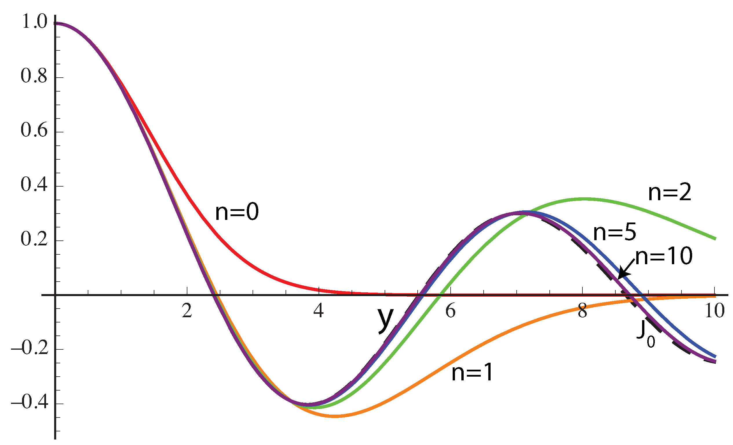
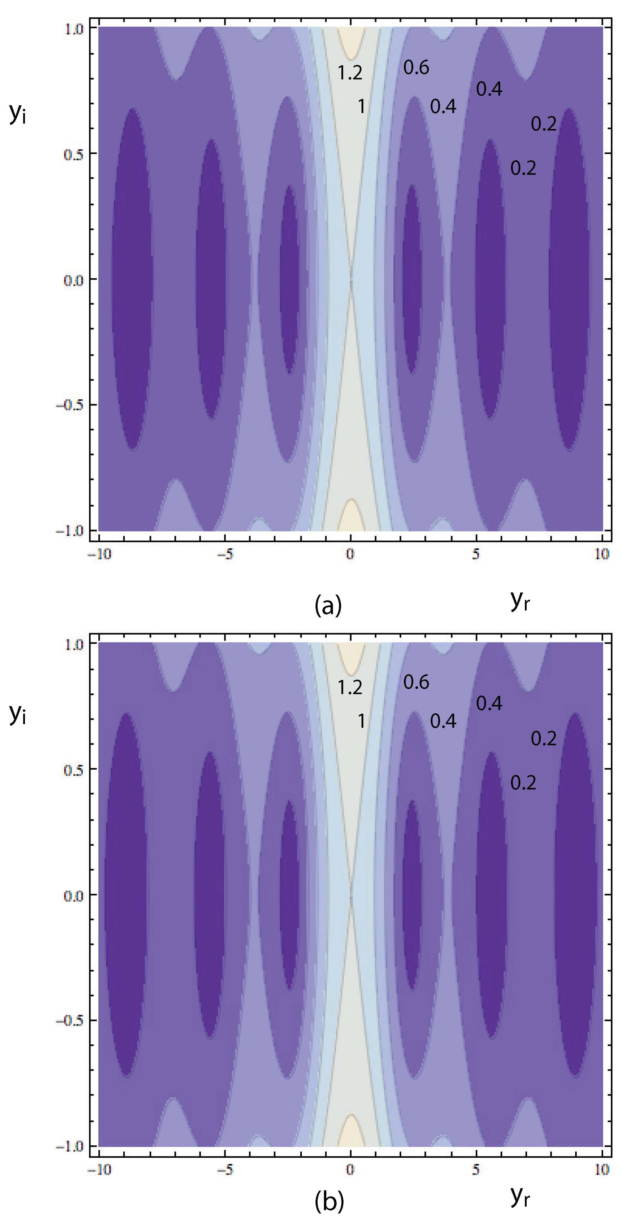
It is seen that for any fixed value of m, the Bessel function can be approximated by Laguerre polynomials of different radial orders n, as n does not appear on the left hand side of Equation (4). To our knowledge, this property has not been described previously. We illustrate the behavior in Figure 1 for the case . It is seen that the Laguerre polynomials approximate to the Bessel function better over a larger domain as the value of n increases. It is seen that the zero and second order terms of the power series expansions for both sides of Equation (4) are the same for all positive values of n (this is true even for any positive m), and more terms match as the value of n increases. This approximation is also valid for complex arguments. In Figure 2, we show contour plots of the modulus of and , illustrating the similarity over the domain shown.
If Stirling’s approximation is used on Equation (3), we obtain the simple form given by Tricomi in 1949 [58],
Equation (5) agrees well with Equation (3) even for small values of n for or 1, but the agreement becomes worse as the value of m increases. Comparison of Equations (1) and (2) with Equation (5) shows that the Stirling approximation has been effectively used in deriving the former two equations.
Mendoza et al. explored approximation of a sLG beam as a Bessel beam using the LSH expression [45]. This relationship can be seen immediately from Equation (4). Chabou and Bencheikh explored the connection between eLG and BG beams [46]. However, the LSH expression is still valid only for , or equivalently, .
A more accurate expression for the generalized Laguerre polynomial was given by Erdélyi [59], which in our terminology is
where . It is seen that both the amplitude and period of the Bessel function vary with v. For small v, the first square bracket becomes equal to unity, and the second square bracket reduces to , so that the expression reduces to
equivalent to Equation (3).
Erdélyi also gave asymptotic expressions, for large n, for the two cases and [59]. Interestingly, these expressions were in terms of Airy functions, suggesting that there may be a connection with Airy beams, another important type of propagationally invariant beam.
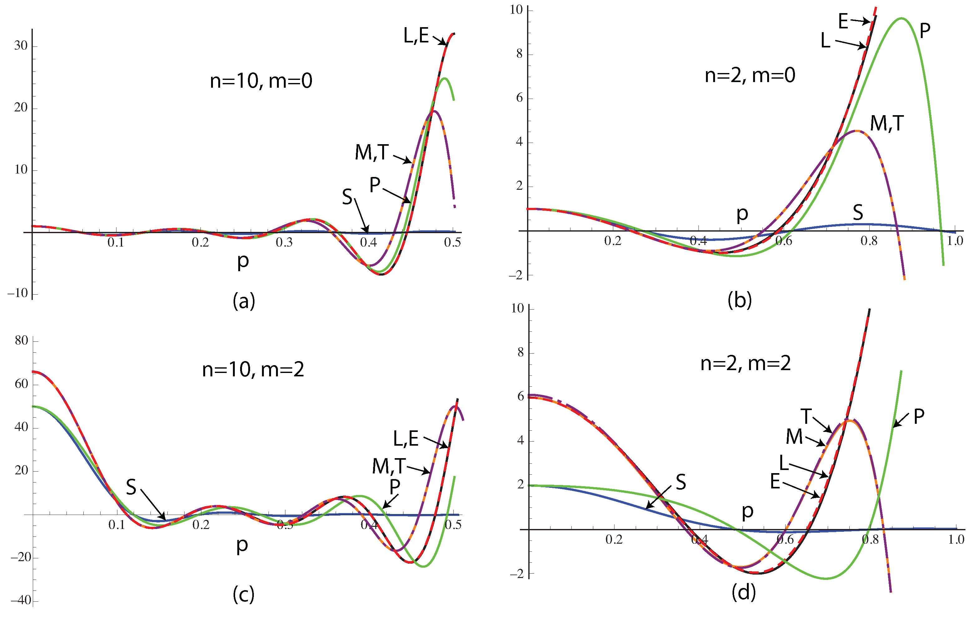
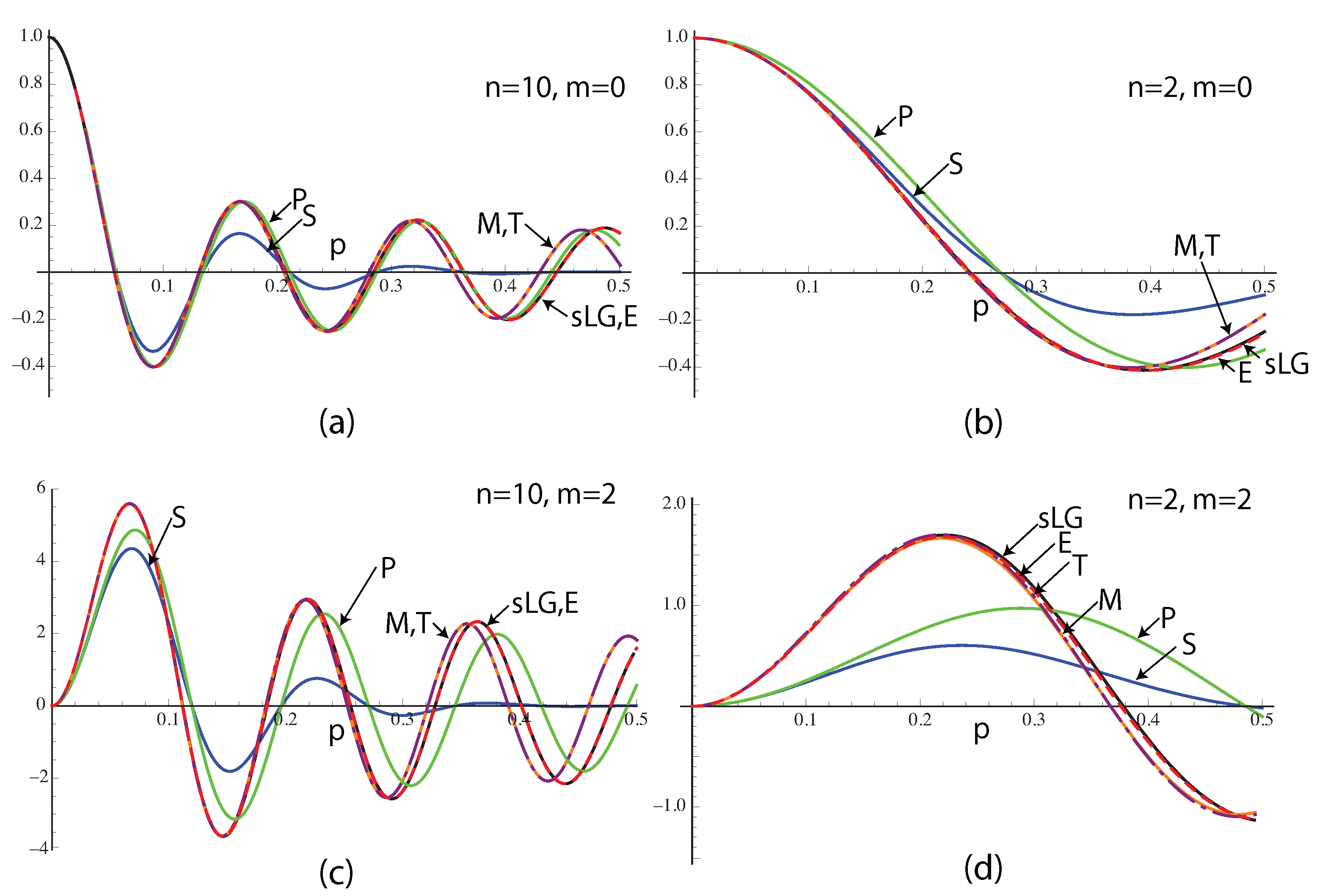
Figure 3 compares the Laguerre polynomials, plotted against p, with the approximations in Equations (1)–(5) (labelled S, P, M, T, E, respectively). For the values shown ( and 2, and 2), Equation (6) (E) agrees very well with the Laguerre polynomial, but tends to break down as p approaches 1. M and T agree with each other, but show some departure from the true values for p greater than about , especially for the case . For , there is a small difference between T and M. For , the value of T shows a slight error, as a result of Stirling’s approximation. The value of S and P at is incorrect for non-zero values of m. Interestingly, S agrees better than P for small values of p for the case .
For , the monotonic regime, the highest power of v dominates (labeled pr, for ‘power’ in Figure 5), and
This equation is valid for complex values of . The two values for depend on the sign of v.
Tricomi gave an asymptotic expression for v real and , which can be written in the form [58]:
where in Tricomi’s case, . The first two terms of the argument of the exponential function tend to cancel for large values of p, so the exponential reduces to a power law. By applying the asymptotic limit for a large argument of the Airy function in Erdélyi’s expression for , we obtain the same expression as in Equation (9), but with
Using Stirling’s approximation, this can be written in terms of a Gamma function, :
or approximately as
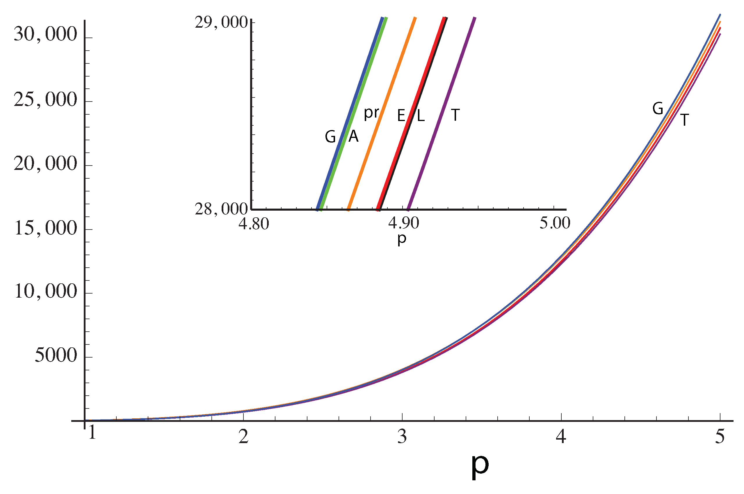
All these expressions for f tend to unity for large n. Their behavior (cases T, E, G, A) is illustrated in Figure 4. An example of comparisons for the different asymptotic expressions for the Laguerre polynomials (T, E, G, A, and also pr) for the case is illustrated in Figure 5. In general, we found from numerical investigation that Erdélyi’s expression gives the best approximation. The power term, labeled pr, Equation (8), only becomes accurate for large values of p, larger for higher values of n. For , at all the approximations except P are within of the correct value, Erdélyi’s expression E is within , but the power term pr is only accurate to within . Nevertheless, the approximation pr is valid in the limit of large p, which is applicable to the angular spectrum of eLG beams [44] or to deLG beams.
An expression analogous to that of Porras et al. for Hermite polynomials, in the context of eHG beams, has been presented in Ref. [18]. Lebedev obtained an asymptotic form valid for both even and odd functions by using Stirling’s formula. This was used to investigate approximation of sHG and eHG beam by cosine-Gauss (cG) beams [46,60]. Asymptotic expressions for even and odd values of n, without using Stirling’s approximation, and therefore valid over a larger range of values of n, were also given by Lebedev [55]. For these, we have
where . More accurate expressions were given earlier by Szegö, where he again calls them formulae of Hilb’s type [57], p. 200. Again, these solutions are valid only for small v, specifically . These can be added in quadrature to produce complex solutions, or proportions summed to give an analogy to Gutiérrez-Vega’s fractional Hermite solutions [38].
For , in similarity with the Laguerre polynomials, we have a simple power term,
Equations analogous to Equation (6) for Hermite polynomials for large, real v can be developed from the expressions for Laguerre polynomials by taking .
It should be noted that for the Hermite and Laguerre cases, the argument of the trigonometrical or Bessel function depends on or N, respectively. It is well known that HG and LG functions are modes of a harmonic oscillator in 1D and 2D, so the in Equations (3) and (13) can be interpreted as representing the zero-point energy. The trigonometrical and Bessel solutions arise for a potential well, equivalent to slab and circular waveguide modes, respectively. So these equations show that the scale of the trigonometric or Bessel function in the solution varies according to the mode numbers, i.e., the potential well varies in width with energy. Further, these scalings are consistent with the second-moment beam widths of sHG and sLG modes given by Carter, and by Phillips and Andrews, respectively [61,62].
3. Bessel-Gauss Beams and Laguerre-Gauss Beams
The gHG, gLG beams (in Cartesian coordinates or cylindrical coordinates ) are given by [18]
where , , , and , and the topological charge m is positive. For gHG, Cartesian coordinates have been used, whereas for gLG, cylindrical coordinates have been used. The parameter c is in general complex, which allows for translating the beam axially so that the waist does not coincide with . The parameter c has been chosen so that, for real c, the dual of a beam is given by changing the sign of c, so the parameter c reflects an important translational symmetry of the beams. Standard beams are given by , elegant beams by and the duals of elegant beams by . For , the beam tends to a Gaussian. If , it is seen that is real for all z, but for other values of c, the argument of the Laguerre polynomial is in general complex. If the argument of the Hermite or Laguerre polynomials tends to infinity, then, using Equations (8) and (14),
Note that has canceled out these expressions, so they are independent of the value of c. Further, for gLG we have taken the positive exponent. For HG, the intensity is a Gaussian modified to give a dark center. There are even and odd solutions according to the value of n. For LG, there is an annular vortex field. In particular, these expressions apply for the far field of eLG or the near field of deLG. More generally, they apply for , Z small, or for , Z large.
Either gHG or gLG can be written in terms of confluent hypergeometric functions. For gLG we have
Different approximations to the amplitude in the waist of sLG and eLG beams are compared in Figure 6 and Figure 7, respectively, plotted against p. In both cases, but especially for eLG (and even more so as c increases further), the increase in the value of the Laguerre polynomial with p is overcome by the decay of the Gaussian. A Gaussian is often assumed to take approximately zero value for an argument greater than three, where its value is less than . According to this approximation, the intensity of the gLG beam drops to zero at , or for sLG, and for eLG. Thus, for large n, the form of asymptotic expression is only relevant for comparatively small values of p. In summary, the approximation E, due to Erdélyi, Equation (6), is excellent even for , and approximations M and T (Equations (5) and (9), respectively) are also good.
Turning now to the cG beam, this is
where are the corresponding values of ; b is a scaling parameter; and A is the amplitude of the beam.
The dual of cG (dcG) is a hyperbolic cosine Gaussian (chG). The dual of BG is [18,33]
where is a modified Bessel function, and the quantity in the first square brackets is approximately constant () for large real arguments. The exponential function then represents an annular beam, with , giving
The waist of dBG is a ring convolved with a two-dimensional Gaussian, equal to the product of a modified Bessel function and a Gaussian, which thus approximates to an annulus with a Gaussian cross-section. An approximation to the dual of a Bessel beam can be efficiently generated experimentally using a combination of an axicon and a lens [29].
4. Aproximating a Laguerre-Gauss Beam by a Bessel-Gauss Beam
We can now use the approximations for the Hermite or Laguerre polynomials for large n, given in Equations (3) and (13), and match the arguments of the factors with those for cG or BG. We start with the HG case. For the Gaussian factor for gHG, we obtain
If , corresponding to eHG, this equation is satisfied for all z if . Note that . Taking is seen to match the waist and far-field (and all intermediate regions) simultaneously [44].
For the cosine factors of cG and gHG,
giving for , agreeing with Ref. [46]. The importance for optics of these results is that large values of , corresponding to large values of n, describe an approximately propagationally invariant beam.
For other values of c, the Gaussian factor does not match for all z, but we can choose to match, for example in the waist, giving for the gHG case
Then the value of A is
or for the special case of eHG, , . To show that this value of A is valid for all z for is a little more difficult, but this can be accomplished using the asymptotic expansions, valid for large n,
For deHG, , then is negative, corresponding to a cosh-Gaussian beam (chG), which has an annular form in the waist. In this case, the asymptotic form for large z, Equation (14), is appropriate.
An advantage of considering the generalized beams, is that b is in general not an integer, but for traditional HG modes n is an integer, so choosing c to be close to 1 allows a traditional gHG beam to be fitted to an arbitrary cG beam [18]. If we match to a cG beam with large , this corresponds to small c, so that , i.e., a high order sHG beam is an approximation to a cosine beam [45,60], for . A truncated cosine beam is therefore an even better approximation to a sHG beam [45,60], which exhibits, over a limited range, propagational invariance and beam regeneration in a scattering medium such as atmospheric turbulence.
For the gLG case, the arguments of the Gaussians are the same as for gHG, so eLG matches BG for all z, with . For gLG, matching at the waist,
The value of A is
Explicitly, in the waist,
where .
For the special case eLG, , and , which can be shown to be valid for all z for large n, using the asymptotic expansions
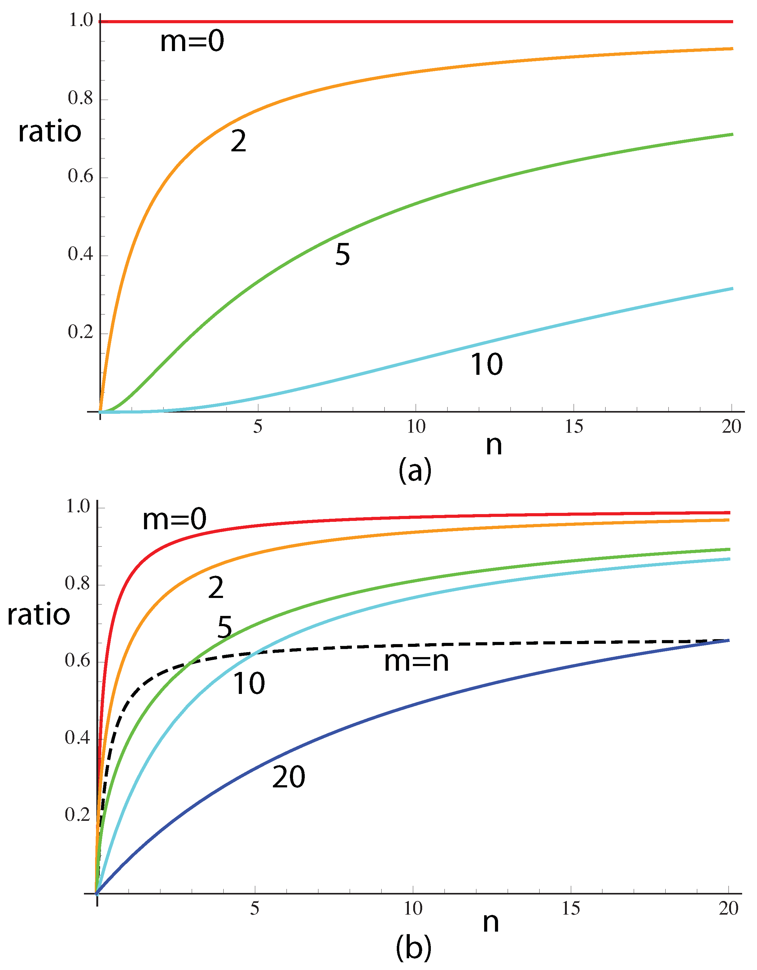
Porras et al. found that, according to their asymptotic expression, [44]. The ratio of their value to that based on the LSH model is shown in Figure 8a. The agreement is exact for , but becomes worse as m is increased. This behavior occurs because Stirling’s approximation was effectively assumed. We also have, for the LSH model applied to eLG, , agreeing with Ref. [46]. As for the HG case, large and n corresponds to an approximately propagationally invariant beam. The result for b of Porras et al. is slightly different [44], as they assume and neglect the zero-point energy. The ratio of the corresponding values of b, , (i.e., the ratio of the inverse widths of the Bessel function) is shown in Figure 8b. For , the agreement is within for , i.e., , and within for . For other values of m, the agreement is much worse: even for , the values agree to within only for . Figure 8b also shows the ratio of the widths for . Now, the ratio saturates to a constant value for large n. The values for large n do not agree to within unless .
In analogy to the result for 2D [45,60], a high order sLG beam is an approximation to a Bessel beam, for . A truncated Bessel beam is therefore a good approximation to a sLG beam, which exhibits, over a limited range, propagational invariance and beam regeneration in a scattering medium. For , the similarity between BG and eLG in this case becomes stronger, and as c becomes even larger, the similarity between BG and gLG continues to increase, until as , they both tend to Gaussians. For , dBG is a good approximation to deLG.
5. Beam Widths and Beam Propagation Factors
Porras et al. derived the correct expression for the second-moment widths of eLG in the near- and far-fields, and also the corresponding values of [44]. They are
Borghi and Santarsiero derived the near-field and far-field widths, and also , for BG beams [63]. Using the value for b equal to , we obtain
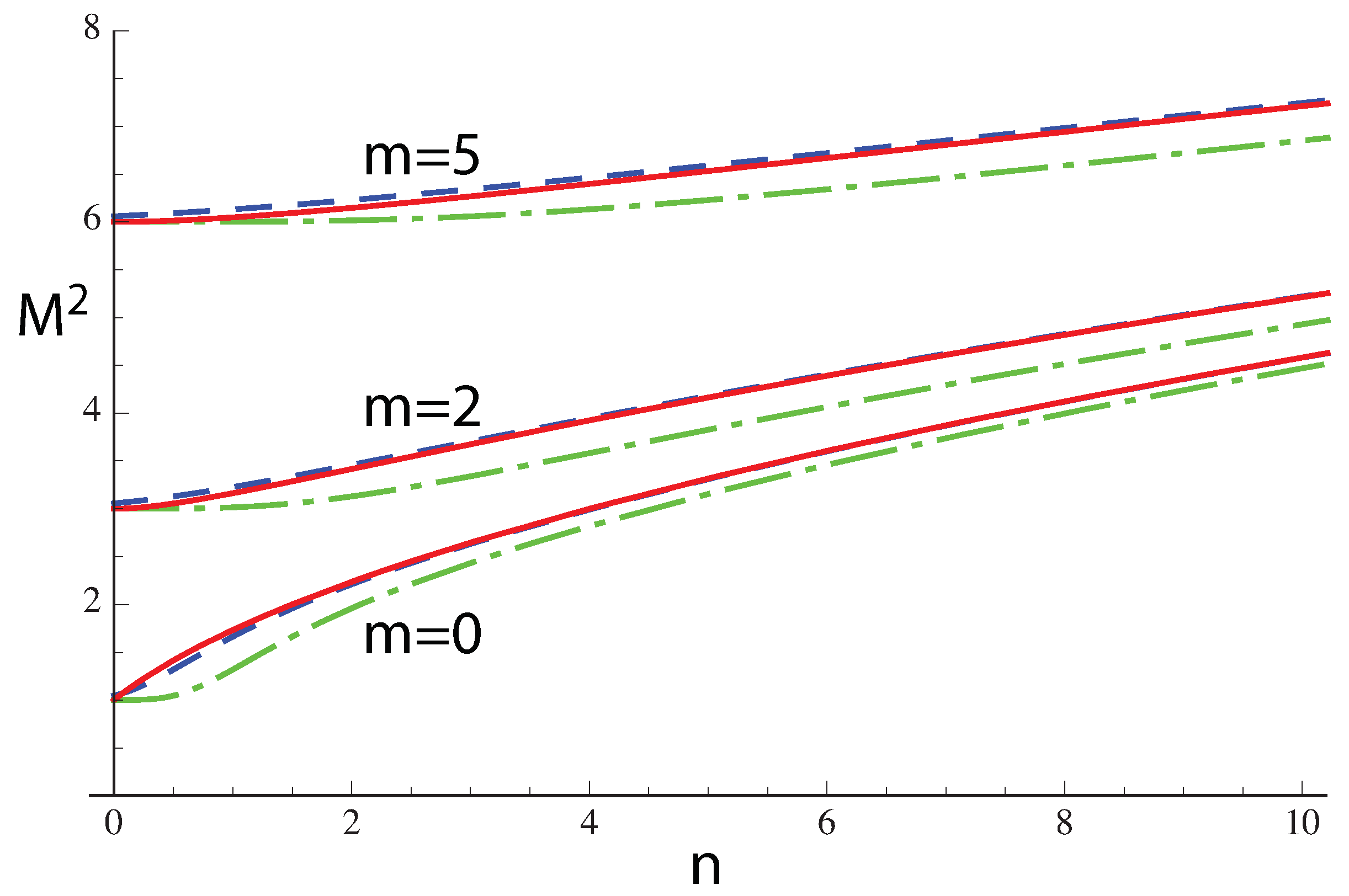
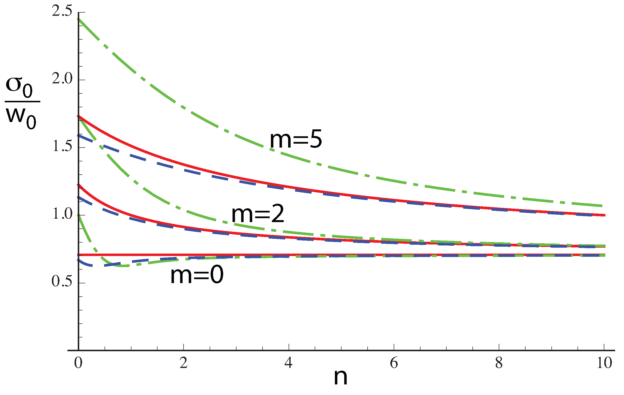
The corresponding behaviors of are shown in Figure 9. The agreement between the values of for eLG and BG are good, even for small values of n, such as . We also show the value of for BG as predicted by Porras et al., which does not agree so well, especially for larger values of m.
But does not tell the whole story, so in Figure 10 we show the second-moment width in the waist, normalized by . Again, the present approximation for BG in Equation (34) agrees very well, even for small n, but the aproximation of Porras et al. is much worse for higher values of m.
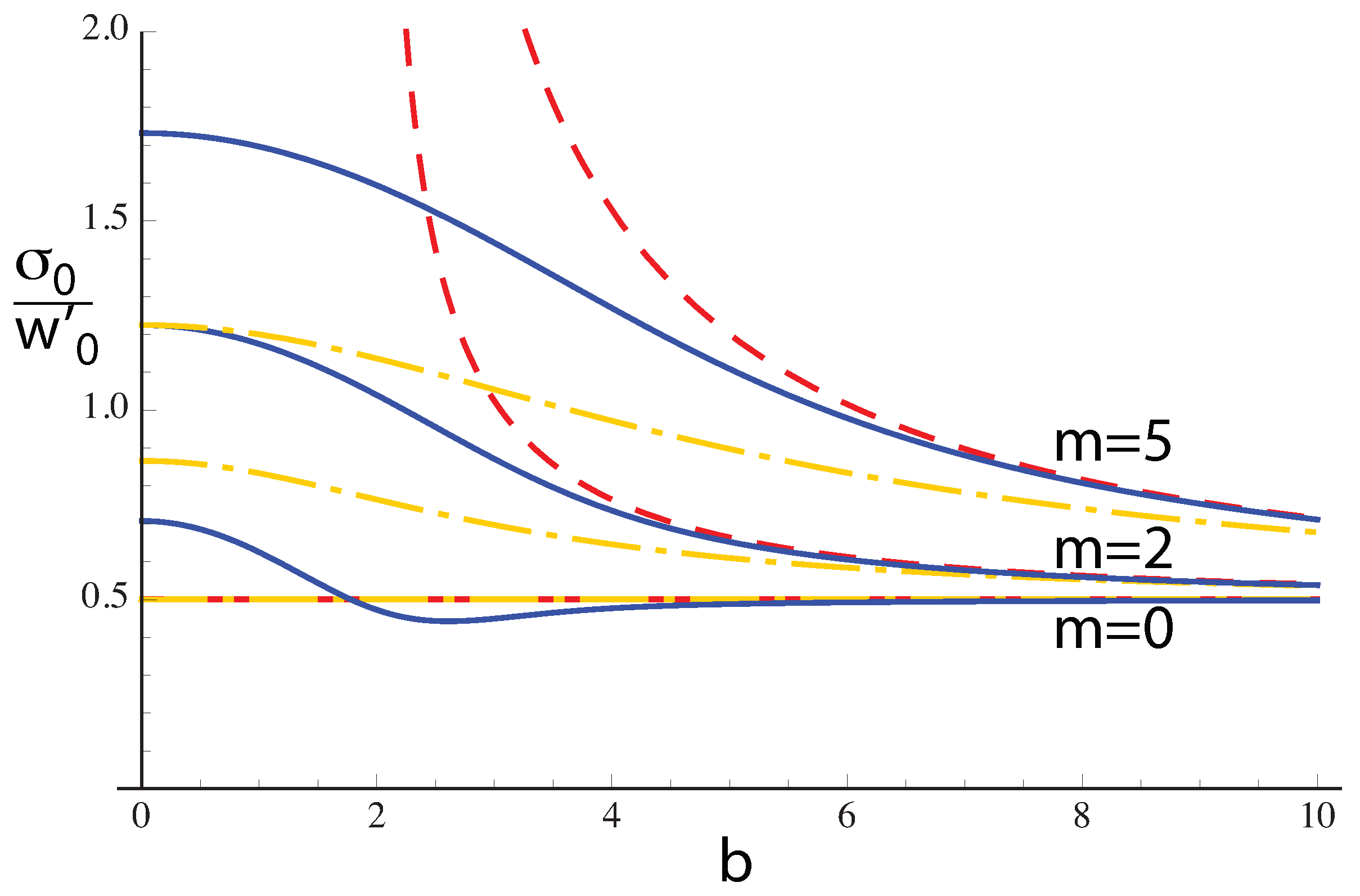
Often, we are interested in the opposite case of approximating a Bessel–Gauss beam by an eLG beam. In Figure 11, we show the second-moment width of Bessel–Gauss beams as a function of the parameter b. The value corresponds to a Gaussian beam. The case of large b tends towards a Bessel beam, but the corresponding second-moment width tends to a value fixed by the width of the underlying Gaussian, which is a constant. This behavior occurs because the second-moment width of a pure Bessel beam is infinite, caused by the strong outer rings.
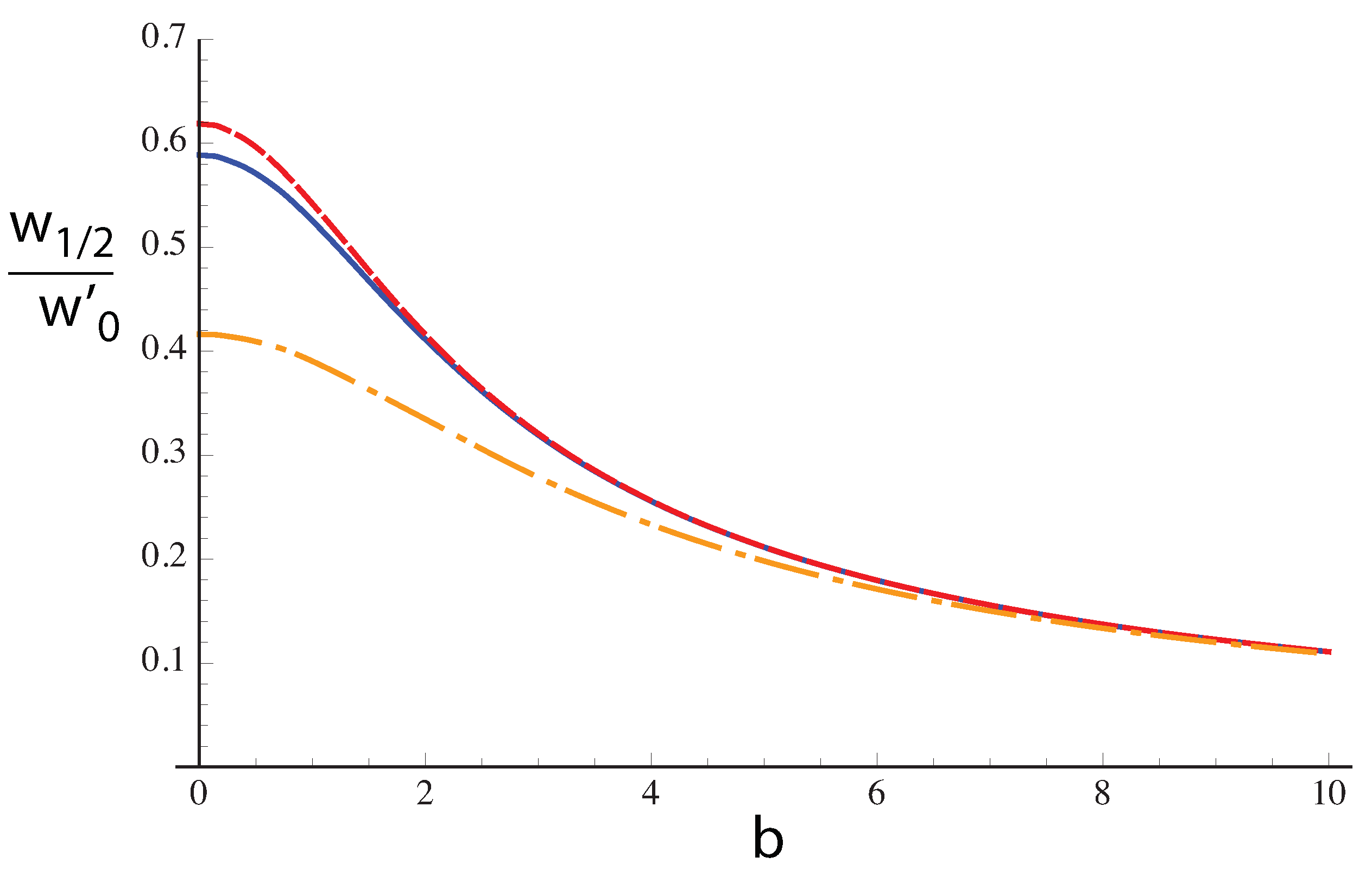
The most important property of a Bessel beam is that its central structure is propagationally invariant, so perhaps a more useful measurement of width for is given by the width where the central lobe intensity falls to one half, the half-width at half maximum (HWHM), . The normalized HWHM is shown in Figure 12. Again we show the cases of BG, and the eLG approximations of the present model and that of Porras et al. [44]. The HWHM tends to zero as b becomes large. The present approximate form of eLG, based on LSH, agrees well even for , corresponding to . In the plot, we do not assume that n is an integer, so that the Laguerre function does not necessarily degenerate to a polynomial.
If we want to use a traditional Laguerre polynomial, we can take , an integer, so that between and (corresponding, for , to and , respectively), c is taken as
The resultant HWHM then agrees with that of BG within for any value of b. The agreement is so good that the corresponding plot is indistinguishable from that for BG in Figure 12.
6. Variation with the Azimuthal Mode Number
So far, we have restricted our study to moderately small values of the azimuthal orders, m. While these values are useful for investigating nonparaxial focusing effects [64], for example, there is also an interest in large values of m, for detection of spinning objects [48], in high-harmonic generation [49], for multiplexing in communication systems [47], and in quantum optics [50,65] and quantum cryptography. Although Equation (3) does not assume that like Equation (2), as the topological charge m increases, then the peak in amplitude in the waist of eLG moves to higher values of p, and we can see from Equation (6), that the LSH model then tends to break down. We find that the approximation of LSH for eLG, although it predicts approximately the correct shape of the amplitude variation, does not give good agreement for the position, width or height of the peak. For large n, the peak of the envelope for gLG occurs at
Assuming that the peak is narrow enough that the second square bracket in Equation (6) is constant and equal to
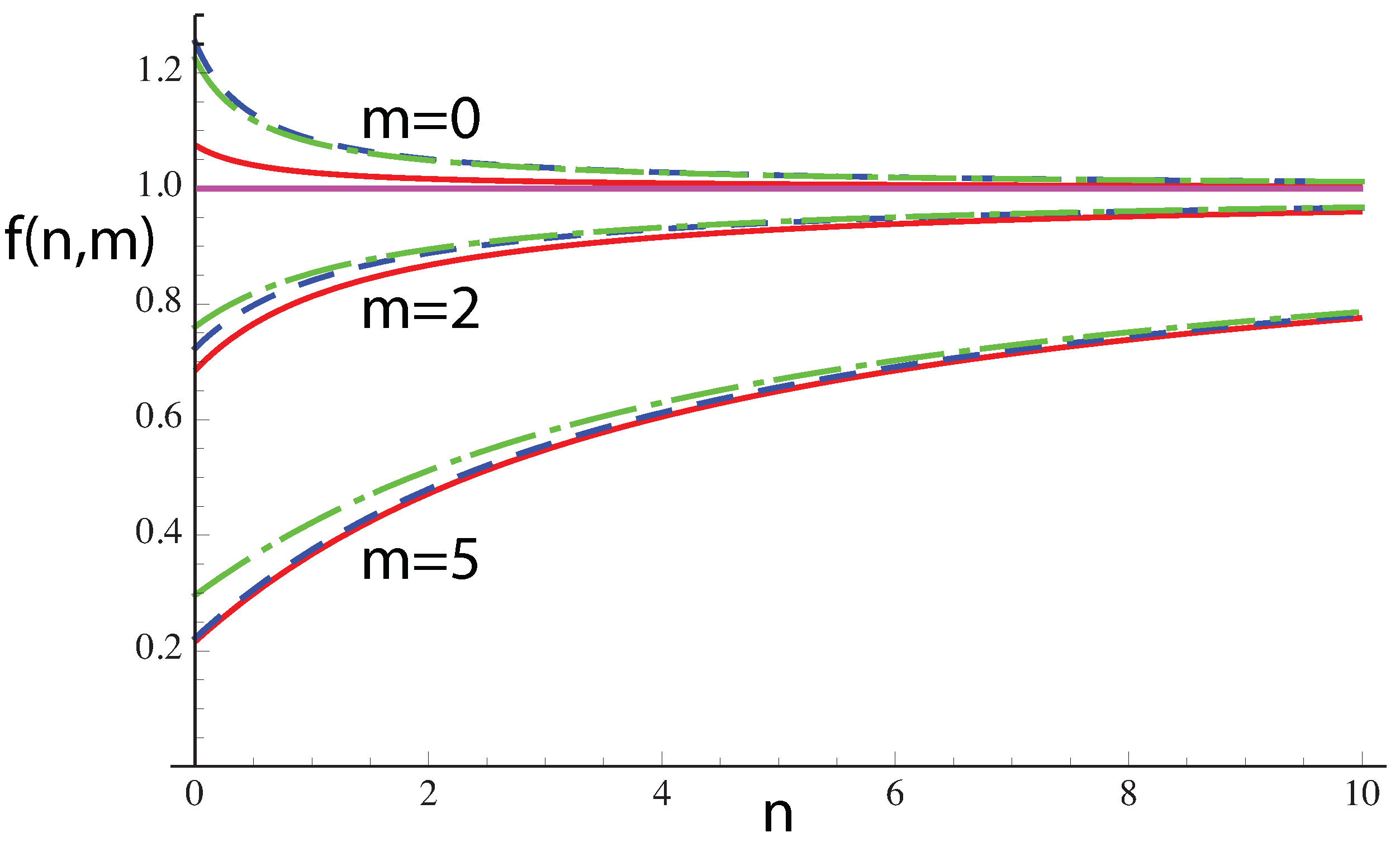
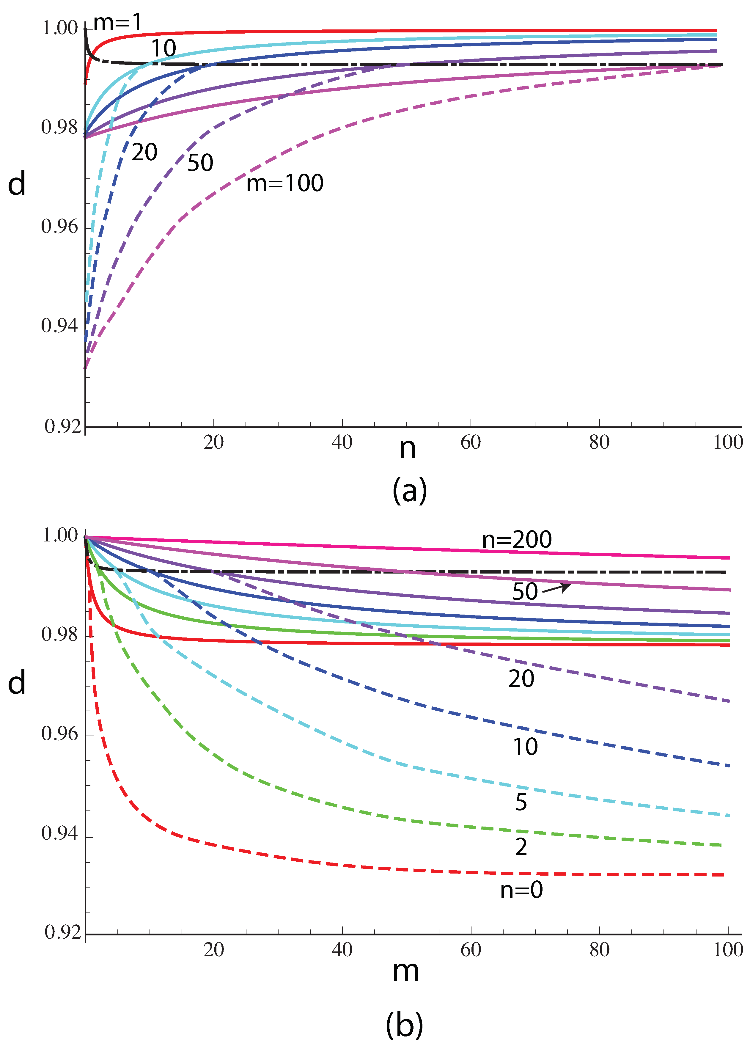
the width of the Bessel function is changed relative to the Gaussian. Then, the rescaled Bessel function width is , so . We show the value of this scaling factor d as solid lines in Figure 13, for values of n and m in the domain . The value of d is quite close to unity, but has a significant effect on the position of the peak in eLG. For , d is constant 0.9929) over a wide range of values of , as shown by the chained lines in Figure 13.
If m is not too large, we find that the approximations , hold. For , then as increase, this approximation predicts that , as compared with for the approximation of Mendoza, and for the approximation of Porras.
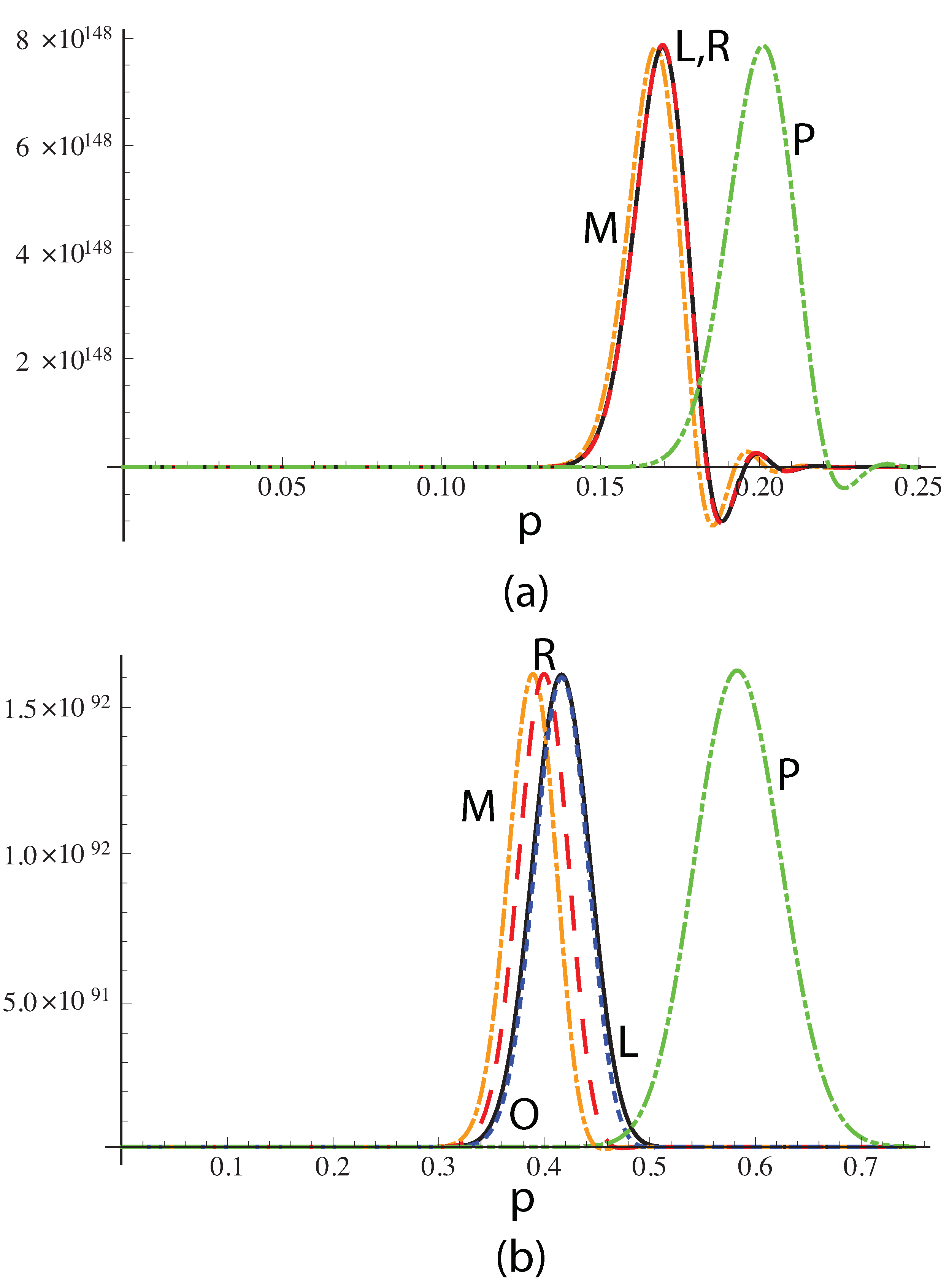
For , we have found empirically that this rescaling still improves the approximation to the waist of a BG beam, but there is a reduced, optimum value of d, as shown by dashed lines in Figure 13. As examples, we show in Figure 14 the amplitude of eLG beams for with (a) and (b) . Different approximations are also shown after equalizing the peak amplitudes, as the absolute values are not correctly predicted. For , the approximation of Mendoza based on LSH (labeled M) is of the correct shape, but shifted towards smaller values of p and slightly narrower. The rescaled version, labeled R, based on Equation (34), is very close to the correct form and position. The values of d are 1 (M), 0.9993 (R), (P). The corresponding values of b are 34.70 (M), 34.45 (R) and 20 (P). For , the rescaled approximation is better than the approximation of Mendoza, but the numerically optimized value of d gives a better fit. The values of d are 1 (M), 0.982 (R), 0.954 (O—optimized), 0.638 (P). The corresponding values of b are 22 (M), 21.61 (R), 20.99 (O) and 8.94 (P). For this case, the sidelobes are very weak, so the beam is not propagationally invariant, as expected from the comparatively small value of n.
7. Expansion in Laguerre-Gauss Modes
The Laguerre polynomials for fixed m are orthogonal with a Gaussian weighting. In fact, the sLG modes are a complete set that can be used to expand a BG beam. Indeed, this was the way the formula for propagation of a BG beam was calculated in Ref. [2].
Here, we generalize the result in Ref. [2], which was for , to arbitrary, integral values of m. Equation 22.9.16 of [35] gives an expansion that can be written in the form
where , and we have summed over orders , to distinguish from . Note that the summation includes values of , whereas Yu et al. used only in their expansion [66]. Equation (7) is valid for different scalings of the Laguerre polynomial relative to the Bessel function. Even though the gLG beams are an orthogonal set only for sLG (), for expansion of the waist of a BG beam in terms of gLG beams, each side must be multiplied by the same Gaussian, which requires that . Then, from Equation (16), we have for a BG beam,
This gives an expansion for a BG beam in terms of gLG components for a constant value of c. Interestingly, the value of c does not affect the relative strengths of the gLG components, which are the same as for a Poisson distribution with parameter and index . Therefore, the strength of the modes for a given m exhibits a peak in the mode number , with an expected value of . As b increases, the strength of the modes tends towards a normal distribution with a coefficient of variation that tends to zero.
8. Discussion
We have compared the performance of different asymptotic expressions for Laguerre polynomials in approximating generalized Laguerre–Gauss beams by Bessel–Gauss beams, and vice versa. The approximation using the Lebedev–Szegö–Hilb expression, as used by Mendoza-Hernandez et al. and Chabou and Bencheikh [45,46], is good for all propagation distances, even for low radial orders n, for elegant Laguerre–Gauss beams (). An arbitrary Bessel–Gauss beam requires a non-integral order n elegant Laguerre–Gauss beam to fit, but for low orders, generalized beams of integer order fit better near the waist. If the value of c is further increased, the fit between gLG and BG is even better than for eLG, but the beams tend to lose their propagational invariance property.
However, the Lebedev–Szegö–Hilb approximation tends to become inaccurate for large values of topological charge, whilst keeping n constant. We have shown that, for , the agreement becomes better after rescaling the argument of the Bessel function according to a function of the mode numbers , although the absolute value is no longer correctly predicted. If , the approximation can be further improved by numerically optimizing the rescaling factor.
Analogous results for Hermite polynomials, and their application to Hermite–Gauss and cosine-Gauss beams has also been presented.
Author Contributions
Conceptualization, C.J.R.S. and M.A.P.; methodology, C.J.R.S. and M.A.P.; software, C.J.R.S.; writing—original draft preparation, C.J.R.S.; writing—review and editing, M.A.P.; visualization, C.J.R.S. All authors have read and agreed to the published version of the manuscript.
Funding
This research received no external funding.
Institutional Review Board Statement
Not applicable.
Informed Consent Statement
Not applicable.
Data Availability Statement
No new data were created.
Conflicts of Interest
The authors declare no conflict of interest.
Abbreviations
The following abbreviations are used in this manuscript:
| BG | Bessel–Gauss |
| cG | cosine-Gauss |
| dBG | dual of Bessel–Gauss |
| deHG | dual of elegant Hermite–Gauss |
| deLG | dual of elegant Laguerre–Gauss |
| dgHG | dual of generalized Hermite–Gauss |
| dgLG | dual of generalized Laguerre–Gauss |
| eHG | elegant Hermite–Gauss |
| eLG | elegant Laguerre–Gauss |
| E | Erdélyi |
| gHG | generalized Hermite–Gauss |
| gLG | generalized Laguerre–Gauss |
| HWHM | Half-width at half-maximum |
| HG | Hermite-Gauss |
| LG | Laguerre–Gauss |
| LSH | Lebedev–Szegö–Hilb |
| M | Mendoza |
| pr | power |
| P | Porras |
| sHG | standard Hermite–Gauss |
| sLG | standard Laguerre–Gauss |
| S | Saghafi |
| T | Tricomi |
References
- Kogelnik, H.; Li, T. Laser beams and resonators. App. Opt. 1966, 5, 1550–1567. [Google Scholar] [CrossRef]
- Sheppard, C.J.R.; Wilson, T. Gaussian-beam theory of lenses with annular aperture. IEE J. Microwaves Opt. Acoust. 1978, 2, 105–112. [Google Scholar] [CrossRef]
- Gori, F.; Guattari, G.; Padovani, C. Bessel-Gauss beams. Opt. Commun. 1987, 64, 491–495. [Google Scholar] [CrossRef]
- Durnin, J. Exact solutions for nondiffracting beams. I. The scalar theory. J. Opt. Soc. Am. A 1987, 4, 651–654. [Google Scholar] [CrossRef]
- Allen, L.; Beijersbergen, M.W.; Spreeuw, R.J.C.; Woerdman, J.P. Orbital angular momentum of light and the transformation of Laguerre-Gaussian laser modes. Phys. Rev. A 1992, 45, 8185–8189. [Google Scholar] [CrossRef]
- Soskin, M.S.; Vasnetsov, M.V. Singular optics. In Progress in Optics; Wolf, E., Ed.; Elsevier: Amsterdam, The Netherlands, 2000; Volume 42, pp. 219–276. [Google Scholar]
- Casperson, L.W.; Hall, D.G.; Tovar, A.A. Sinusoidal-Gaussian beams in complex optical systems. J. Opt. Soc. Am. A 1997, 14, 3341–3348. [Google Scholar] [CrossRef]
- Abramochkin, E.; Volostnikov, V. Beam transformations and nontransformed beams. Opt. Commun. 1991, 83, 123–135. [Google Scholar] [CrossRef]
- Kimel, I.; Elias, L.R. Relations between Hermite and Laguerre Gaussian modes. IEEE J. Quant. Elect. 1993, 29, 2562–2567. [Google Scholar] [CrossRef]
- Siegman, A.E. Hermite-Gaussian functions of complex arguments as optical-beam eigenfunctions. J. Opt. Soc. Am. 1973, 63, 1093–1094. [Google Scholar] [CrossRef]
- Zauderer, E. Complex argument Hermite-Gaussian and Laguerre-Gaussian beams. J. Opt. Soc. Am. A 1986, 3, 465–469. [Google Scholar] [CrossRef]
- Wünsche, A. Generalized Gaussian beam solutions of paraxial optics and their connections to a hidden symmetry. J. Opt. Soc. Am. A 1989, 6, 1320–1329. [Google Scholar] [CrossRef]
- Saghafi, S.; Sheppard, C.J.R. Near field and far field of elegant Hermite-Gaussian and Laguerre-Gaussian modes. J. Mod. Opt. 1998, 45, 1999–2009. [Google Scholar] [CrossRef]
- Shin, S.Y.; Felsen, L. Gaussian beam modes by multipoles with complex source points. J. Opt. Soc. Am. 1977, 67, 699–700. [Google Scholar] [CrossRef]
- Enderlein, J.; Pampaloni, F. Unified operator approach for deriving Hermite-Gaussian and Laguerre-Gaussian laser modes. J. Opt. Soc. Am. A 2004, 21, 1553–1558. [Google Scholar] [CrossRef]
- Wünsche, A. Analogien zwischen ausserordentlichen und ordentlichen Wellen nach nichtorthogonaler Koordinatentransformation und die parabolischen Näherungsgleichungen. Ann. Phys. 1970, 25, 113–135. [Google Scholar] [CrossRef]
- Pratesi, R.; Ronchi, L. Generalized Gaussian beams in free space. J. Opt. Soc. Am. 1977, 67, 1274–1276. [Google Scholar] [CrossRef]
- Sheppard, C.J.R. Beam duality, with application to generalized Bessel-Gaussian, and Hermite- and Laguerre-Gaussian beams. Opt. Exp. 2009, 17, 3690–3697. [Google Scholar] [CrossRef]
- Rayleigh, J.W.S. On the diffraction of object glasses. Mon. Notes R. Astronom. Soc. 1872, 33, 59–63. [Google Scholar]
- Airy, G.B. On the diffraction of an annular aperture. Phil. Mag. Ser. 3 1841, 18, 1–10. [Google Scholar]
- Steward, G. IV Aberration diffraction effects. Phil. Trans. R. Soc. Lond. Ser. A 1926, 225, 131–198. [Google Scholar]
- Sheppard, C.J.R. Electromagnetic field in the focal region of wide-angular annular lens and mirror systems. IEE J. Microw. Opt. Acoust. 1978, 2, 163–166. [Google Scholar] [CrossRef]
- Durnin, J.; Miceli, J.J., Jr.; Eberly, J.H. Diffraction-free beams. Phys. Rev. Lett. 1987, 58, 1499–1501. [Google Scholar] [CrossRef]
- Sheppard, C.J.R.; Choudhury, A. Annular pupils, radial polarization, and superresolution. App. Opt. 2004, 43, 4322–4327. [Google Scholar] [CrossRef] [PubMed]
- Sheppard, C.J.R.; Balla, N.K.; Rehman, S.; Yew, E.Y.S.; Tang, W.T. Bessel beams with the tightest focus. Opt. Commun. 2009, 282, 4647–4656. [Google Scholar] [CrossRef]
- Wang, H.F.; Gan, F. High focal depth with a pure-phase apodizer. App. Opt. 2001, 40, 5658–5662. [Google Scholar] [CrossRef] [PubMed]
- Mondal, A.; Yevick, A.; Blackburn, L.C.; Kanellakoupoulos, N.; Grier, D.G. Projecting non-diffracting waves with intermediate-plane holography. Opt. Exp. 2018, 26, 3926–3931. [Google Scholar] [CrossRef]
- McLeod, J.H. The Axicon: A New Type of Optical Element. J. Opt. Soc. Am. 2004, 44, 592–597. [Google Scholar] [CrossRef]
- Arimoto, R.; Saloma, C.; Tanaka, T.; Kawata, S. Imaging properties of axicon in a scanning optical system. App. Opt. 1992, 31, 6653–6657. [Google Scholar] [CrossRef]
- Breen, T.; Basque-Giroux, N.; Fuchs, U.; Golub, I. Tuning the resolution and depth of field of a lens using an adjustable ring beam illumination. App. Opt. 2020, 59, 4744–4749. [Google Scholar] [CrossRef]
- Miller, W. Symmetry and Separation of Variables, 4th ed.; Addison-Wesley: Reading, MA, USA, 1977. [Google Scholar]
- Bandres, M.A.; Gutiérrez-Vega, J.C. Cartesian beams. Opt. Lett. 2007, 32, 3459–3461. [Google Scholar] [CrossRef]
- Karimi, E.; Zito, G.; Piccirillo, B.; Marrucci, L.; Santamato, E. Hypergeometric-Gaussian beams. Opt. Lett. 2007, 32, 3053–3055. [Google Scholar] [CrossRef]
- Kotlyar, V.V.; Kovalev, A.A. Family of hypergeometric laser beams. J. Opt. Soc. Am. A 2008, 25, 262–270. [Google Scholar] [CrossRef] [PubMed]
- Abramowitz, M.; Stegun, I. Handbook of Mathematical Functions, 3rd ed.; Dover: New York, NY, USA, 1972. [Google Scholar]
- Torre, A. A note on the general solution of the paraxial wave equation: A Lie algebra view. J. Opt. A Pure Appl. Opt. 2008, 10, 055006. [Google Scholar] [CrossRef]
- Bandres, M.A.; Guizar-Sicairos, M. Paraxial group. Opt. Lett. 2009, 34, 13–15. [Google Scholar] [CrossRef] [PubMed]
- Gutiérrez-Vega, J.C. Fractionalization of optical beams: I. Planar analysis. Opt. Lett. 2007, 32, 1521–1523. [Google Scholar] [CrossRef]
- Gutiérrez-Vega, J.C. Fractionalization of optical beams: II. Elegant Laguerre–Gaussian modes. Opt. Exp. 2007, 15, 6300–6313. [Google Scholar] [CrossRef]
- Whittaker, E.T.; Watson, G.N. A Course of Modern Analysis, 4th ed.; Cambridge University Press: Cambridge, UK, 1927. [Google Scholar]
- Whittaker, E.T. An expression of certain known functions as generalized hypergeometric functions. Bul. Am. Math. Soc. 1903, 10, 125–134. [Google Scholar] [CrossRef]
- Lopez-Mago, D.; Bandres, M.A.; Gutiérrez-Vega, J.C. Propagation of Whittaker-Gauss beams. Proc. SPIE 2009, 7430, 743013. [Google Scholar]
- Bagini, V.; Frezza, F.; Santarsiero, M.; Schettini, G.; Shirripa Spagnolo, G. Generalized Bessel-Gauss beams. J. Mod. Opt. 1996, 43, 1155–1166. [Google Scholar]
- Porras, M.A.; Borghi, R.; Santarsiero, M. Relationship between elegant Laguerre-Gauss and Bessel-Gauss beams. J. Opt. Soc. Am. A 2001, 18, 177–184. [Google Scholar] [CrossRef]
- Mendoza-Hernandez, J.; Arroyo-Carrasco, M.L.; Iturbe-Castillo, M.D.; Chavez-Cerda, S. Laguerre–Gauss beams versus Bessel beams showdown: Peer comparison. Opt. Lett. 2015, 40, 3739–3742. [Google Scholar] [CrossRef] [PubMed]
- Chabou, S.; Bencheikh, A. Elegant Gaussian beams: Nondiffracting nature and self-healing property. App. Opt. 2020, 59, 9999–10006. [Google Scholar] [CrossRef] [PubMed]
- Gibson, G.; Courtial, J.; Padgett, M.J. Free-space information transfer using light beams carrying orbital angular momentum. Opt. Exp. 2004, 12, 5448–5456. [Google Scholar] [CrossRef] [PubMed]
- Lavery, M.P.J.; Speirits, F.C.; Barnett, S.M.; Padgett, M.J. Detection of a spinning object using light’s orbital angular momentum. Science 2013, 341, 537–540. [Google Scholar] [CrossRef] [PubMed]
- Pandey, A.K.; de las Heras, A.; Larrieu, T.; San Román, J.; Serrano, J.; Plaja, L.; Baynard, E.; Pittman, M.; Dovillaire, G.; Kazamias, S.; et al. Characterization of extreme ultraviolet vortex beams with a very high topological charge. ACS Photonics 2022, 9, 944–951. [Google Scholar] [CrossRef]
- Fickler, R.; Campbell, G.; Buchler, B.; Zeilinger, A. Quantum entanglement of angular momentum states with quantum numbers up to 10,010. Proc. Natl. Acad. Sci. USA 2016, 113, 13642–13647. [Google Scholar] [CrossRef]
- Porras, M. Upper bound to the orbital angular momentum carried by an ultrashort pulse. Phys. Rev. Lett. 2019, 122, 123904. [Google Scholar] [CrossRef]
- Siegman, A.E. New developments in laser resonators. Proc. SPIE 1990, 1224, 2–14. [Google Scholar]
- Saghafi, S.; Sheppard, C.J.R. The beam propagation factor for higher order Gaussian beams. Opt. Commun. 1998, 153, 207–210. [Google Scholar] [CrossRef]
- Saghafi, S.; Sheppard, C.J.R.; Piper, J. Characterising elegant and standard Hermite-Gaussian beam modes. Opt. Commun. 2001, 191, 173–179. [Google Scholar] [CrossRef]
- Lebedev, N.N. Special Functions and Their Applications; Prentice-Hall: Englewood Cliffs, NJ, USA, 1965. [Google Scholar]
- Zou, K.; Pang, K.; Song, H.; Fan, J.; Zhao, Z.; Song, H.; Zhang, R.; Zhou, H.; Minoofar, A.; Liu, C.; et al. High-capacity free-space optical communications using wavelength- and mode-division-multiplexing in the mid-infrared region. Nat. Commun. 2022, 13, 7662. [Google Scholar] [CrossRef] [PubMed]
- Szegö, G. Orthogonal Polynomials; American Mathematical Society: Providence, RI, USA, 1939. [Google Scholar]
- Tricomi, F.G. Sul comportamento asintotico dei polinomi di Laguerre. Ann. Mat. Pura Appl. 1949, 28, 263–289. [Google Scholar] [CrossRef]
- Erdélyi, A. Asymptotic forms for Laguerre polynomials. J. Indian Math. Soc. 1961, 24, 235–250. [Google Scholar]
- Bencheikh, A.; Forbes, A. The non-diffracting nature of truncated Hermite–Gaussian beams. J. Opt. Soc. Am. A 2020, 37, C1–C6. [Google Scholar] [CrossRef]
- Carter, W.H. Spot size and divergence for Hermite Gaussian beams of any order. App. Opt. 1980, 19, 1027–1028. [Google Scholar] [CrossRef]
- Phillips, R.L.; Andrews, L.C. Spot size and divergence for Laguerre Gaussian beams of any order. App. Opt. 1983, 22, 643–644. [Google Scholar] [CrossRef]
- Borghi, R.; Santarsiero, M. M2 factor of Bessel-Gauss beams. Opt. Lett. 1997, 22, 262–264. [Google Scholar] [CrossRef] [PubMed]
- Sheppard, C.J.R. Polarized focused vortex beams: Half-order phase vortices. Opt. Exp. 2014, 22, 18128–18141. [Google Scholar] [CrossRef]
- Molina-Terriza, G.; Torres, J.P.; Torner, L. Management of the angular momentum of light: Preparation of photons in multidimensional vector states of angular momentum. Phys. Rev. Lett. 2001, 88, 013601. [Google Scholar] [CrossRef]
- Yu, L.; Huang, W.; Huang, M.; Zhu, Z.; Zeng, X.; Ji, W. The Laguerre–Gaussian series representation of two-dimensional fractional Fourier transform. J. Phys. A Math. Gen. 1998, 31, 9353–9357. [Google Scholar] [CrossRef]
Figure 1.
Approximations to a Bessel function given by Equation (4), in terms of Laguerre polynomials with different values of the parameter n.
Figure 1.
Approximations to a Bessel function given by Equation (4), in terms of Laguerre polynomials with different values of the parameter n.

Figure 2.
Contour plots of (a) , and (b) the right hand side of Equation (4), in terms of .
Figure 2.
Contour plots of (a) , and (b) the right hand side of Equation (4), in terms of .

Figure 3.
The Laguerre polynomials (L) for (a,c) and (b,d), for (a,b) and (c,d), plotted against . Different approximations are also shown: Saghafi (S) Equation (1); Porras et al. (P) Equation (2); Mendoza (or Lebedev–Szegö–Hilb) (M) Equation (3); Tricomi (T, chained) Equation (5); Erdélyi (E, dashed) Equation (6).

Figure 4.
The factor for different approximations to a Laguerre polynomial for as a function of n with m as parameter. For Tricomi’s case, , has a constant value of unity. For Erdélyi’s case, : solid lines. The Gamma function expression, , is shown as dashed lines. The approximate case, , is shown as chained lines.

Figure 5.
Comparison of the values of the Laguerre polynomial as a function of , labeled L, with approximate expressions due to Tricomi (T), to Erdélyi (E), the Gamma function form (G), the approximation (A), and the power term (pr). The insert shows an enlarged view, illustrating that the Erdélyi expression is closest to the Laguerre polynomial.

Figure 6.
The amplitude of the standard Laguerre0-Gauss beams (sLG) in the waist for (a,c) and 2 (b,d), for (a,b) and 2 (c,d), plotted against p. Different approximations: Saghafi (labeled S) Equation (1), Porras (P) Equation (2), Mendoza (M) Equation (3), Tricomi (T, chained) Equation (5), Erdélyi (E, dashed) Equation (6), are also shown.

Figure 7.
The amplitude of the elegant Laguerre–Gauss beams (labeled eLG) in the waist for (a,c) and 2 (b,d), for (a,b) and 2 (c,d), plotted against p. Different approximations: Saghafi (S) Equation (1), Porras (P) Equation (2), Mendoza (M) Equation (3), Tricomi (T, chained) Equation (5), Erdélyi (E, dashed) Equation (6), are also shown.

Figure 8.
The variations in the ratios for the model of Porras et al. in Ref. [44] to that of the LSH model for (a) the amplitude A, given by , and (b) b for the Bessel function corresponding to an eLG beam, equal to , as functions of n, with m as parameter. The variation for is shown as a dotted line in (b).

Figure 9.
The value of for eLG beams, as a function of n with m as parameter (solid lines). The predictions of Equation (32) (dashed lines) and the Porras et al. model [44] (chained lines) for BG are also shown.

Figure 10.
The normalized width in the waist for eLG beams (solid lines), as a function of n with m as a parameter. The predictions of Equation (32) (dashed lines) and the Porras et al. model of [44] (chained lines) for BG are also shown.

Figure 11.
The normalized second-moment width in the waist for BG beams (solid lines), as a function of b with m as a parameter. The predictions of Equation (32) (dashed lines) and the Porras et al. model of [44] (chained lines) for eLG are also shown.

Figure 12.
The normalized half-width in the waist for BG beams (solid line), as a function of b for . The predictions of Equation (32) (dashed line) and the Porras et al. model [44] (chained line) for eLG are also shown. Fitting a traditional Laguerre polynomial (integral n) to BG using Equation (33). gives a curve indistinguishable from that for BG.

Figure 13.
The scaling factor d for b, (a) as a function of n with m as parameter, and (b) as a function of m with n as parameter. Solid lines correspond to the rescaled case (R), according to Equation (34), and dashed lines to the optimized case (O).
Figure 13.
The scaling factor d for b, (a) as a function of n with m as parameter, and (b) as a function of m with n as parameter. Solid lines correspond to the rescaled case (R), according to Equation (34), and dashed lines to the optimized case (O).

Figure 14.
The amplitude in eLG beams (L) for , with (a) , (b) , solid lines. The approximations of Porras (P, double-chained), Mendoza (M, chained), rescaled (R, dashed), and optimized (O, dotted) are also shown.
Figure 14.
The amplitude in eLG beams (L) for , with (a) , (b) , solid lines. The approximations of Porras (P, double-chained), Mendoza (M, chained), rescaled (R, dashed), and optimized (O, dotted) are also shown.

Disclaimer/Publisher’s Note: The statements, opinions and data contained in all publications are solely those of the individual author(s) and contributor(s) and not of MDPI and/or the editor(s). MDPI and/or the editor(s) disclaim responsibility for any injury to people or property resulting from any ideas, methods, instructions or products referred to in the content. |
© 2023 by the authors. Licensee MDPI, Basel, Switzerland. This article is an open access article distributed under the terms and conditions of the Creative Commons Attribution (CC BY) license (https://creativecommons.org/licenses/by/4.0/).
Share and Cite
MDPI and ACS Style
Sheppard, C.J.R.; Porras, M.A. Comparison between the Propagation Properties of Bessel–Gauss and Generalized Laguerre–Gauss Beams. Photonics 2023, 10, 1011. https://doi.org/10.3390/photonics10091011
AMA Style
Sheppard CJR, Porras MA. Comparison between the Propagation Properties of Bessel–Gauss and Generalized Laguerre–Gauss Beams. Photonics. 2023; 10(9):1011. https://doi.org/10.3390/photonics10091011
Chicago/Turabian StyleSheppard, Colin J. R., and Miguel A. Porras. 2023. "Comparison between the Propagation Properties of Bessel–Gauss and Generalized Laguerre–Gauss Beams" Photonics 10, no. 9: 1011. https://doi.org/10.3390/photonics10091011
Note that from the first issue of 2016, this journal uses article numbers instead of page numbers. See further details here.