Principle and Recent Development in Photonic Time-Stretch Imaging


1
School of Microelectronics, Shenzhen Institute of Information Technology, Shenzhen 518172, China
2
Department of Periodontology, Shenzhen Stomatological Hospital, Southern Medical University, Shenzhen 518005, China
3
Center for Cognition and Neuroergonomics, State Key Laboratory of Cognitive Neuroscience and Learning, Beijing Normal University at Zhuhai, Zhuhai 519087, China
4
School of Engineering and Digital Arts, University of Kent, Canterbury, CT2 7NT, UK
*
Authors to whom correspondence should be addressed.
Photonics 2023, 10(7), 817; https://doi.org/10.3390/photonics10070817
Submission received: 29 May 2023
/
Revised: 15 June 2023
/
Accepted: 18 June 2023
/
Published: 13 July 2023
Abstract
:Inspiring development in optical imaging enables great applications in the science and engineering industry, especially in the medical imaging area. Photonic time-stretch imaging is one emerging innovation that attracted a wide range of attention due to its principle of one-to-one-to-one mapping among space-wavelength-time using dispersive medium both in spatial and time domains. The ultrafast imaging speed of the photonics time-stretch imaging technique achieves an ultrahigh frame rate of tens of millions of frames per second, which exceeds the traditional imaging methods in several orders of magnitudes. Additionally, regarding ultrafast optical signal processing, it can combine several other optical technologies, such as compressive sensing, nonlinear processing, and deep learning. In this paper, we review the principle and recent development of photonic time-stretch imaging and discuss the future trends.
1. Introduction
Recent developments in optical imaging have paved the way for diversified applications in science and industry, especially around medicine, biochemistry, and biology [1,2,3,4,5,6,7,8,9,10,11,12,13,14,15,16,17,18,19,20,21,22,23,24,25,26,27,28]. For example, noninvasive diagnosis of biomedical tissue using optical coherence tomography (OCT) [1,2,3,4,5,6,7,8,9,10], ultrafast optical imaging based on photonic time-stretch structure [10,11,12,13,14,15,16,17,18,19,20,21,22,23,24,25,26,27,28,29,30,31], data compressive optical imaging systems [10,11,12,13,14,15,16,17,18,19,20,21,22], blood screening and abnormal cell screening using contrast microscopy [23,24,25,26,27], these developments of optical imaging are with the support of digital technologies [32,33,34,35,36,37,38,39] and the growing industry.
The developments of optical imaging are mainly two parts. One part is to improve the imaging resolution, either in the spatial domain (spatial resolution) [40,41,42,43,44,45,46,47,48,49,50,51,52,53,54] or the time domain (temporal resolution) [10,11,12,13,14,15,16,17,18,19,20,21,22,23,55,56,57,58,59,60]. The methods of improving the spatial resolution of imaging systems are mainly stochastic optical reconstruction microscopy (STORM) [40,41,42,43] imaging, photoactivated localization microscopy (PALM) [44,45] imaging, structured illumination microscopy (SIM) imaging [48,49,50,51,52,53,54], and stimulated emission depletion (STED) microscopy imaging [55]. The technique of improving the temporal resolution of imaging systems in this review is mainly focused on the photonic time-stretch (PTS) technique [10,11,12,13,14,15,16,17,18,19,20,21,22,23]. The other part is to improve sensitivity and specificity. In order to improve the sensitivity, 2D devices, such as charge-coupled devices (CCD) and complementary metal oxide semiconductors (CMOS), 1D devices, such as photomultiplier tubes (PMT), avalanche photodetector (APD), and infrared-coated photodetector (PD) [60,61] are applied to improve the sensitivity of the imaging system. In order to obtain more specific information on the imaging systems, more techniques such as fluorescence imaging with biomarkers [62,63,64], phase-contrast imaging with interferometric structure for transparent sample imaging [65,66], and polarization-sensitive imaging are employed [67].
Among the improvement of current imaging systems, improving temporal resolution attracts a large amount of attention and obtained fruitful achievement. The most sparking technique for improving temporal resolution for imaging systems is PTS [1,2,3,4,5,6,7,8,9,10,11,12,13,14,15,16,17,18,19,20,21,22,23,24,25,26,27,28,29,30,31,66,67,68,69,70,71,72,73,74]—a technique that encodes the spatial profile of sample imaging information into the temporal profile data for ultrafast imaging using the dispersive medium in both spatial and temporal domains based on the dispersive properties of broadband light. It was proposed and demonstrated by Goda et al. in 2009 for the first time [59]. Additionally, it can achieve a continuous ultrafast imaging speed of millions of frames per second, which is several magnitudes higher compared to traditional imaging techniques. Moreover, due to its inherent nature, it can combine other several recent optical technologies such as compressive sensing [10,11,12,13,14,15,16,17,18,22,29,75,76], nonlinear processing [76,77,78], amplification [4,79], and deep learning [80,81], which are beyond the capabilities of other imaging techniques.
In this paper, we review the principles and applications of time-stretch imaging systems. In Section 2, we review the principles and introduce key components of time-stretch imaging systems. In Section 3, we review serval applications of time-stretch imaging. In Section 4, we discuss the future trends of time-stretch imaging. In Section 5, we summarize this paper.
2. Principles and Key Components
The purpose of PTS imaging is to map the spatial imaging information into the spectrum of the incident broadband-pulsed light. The spectral information, which is already encoded by the spatial imaging information, is time-stretched into 1D temporal profile data. Then the temporal profile data is detected by a single-pixel PD [59]. The two steps of PTS imaging are essential. The first step is called space-to-wavelength conversion, which maps the spatial imaging information into the spectrum of incident broadband-pulsed light using spatial dispersive devices in the spectral domain. The second step is called wavelength-to-time conversion, which maps the imaging-encoded spectral information into 1D temporal profile data using temporal dispersive devices in the time domain.
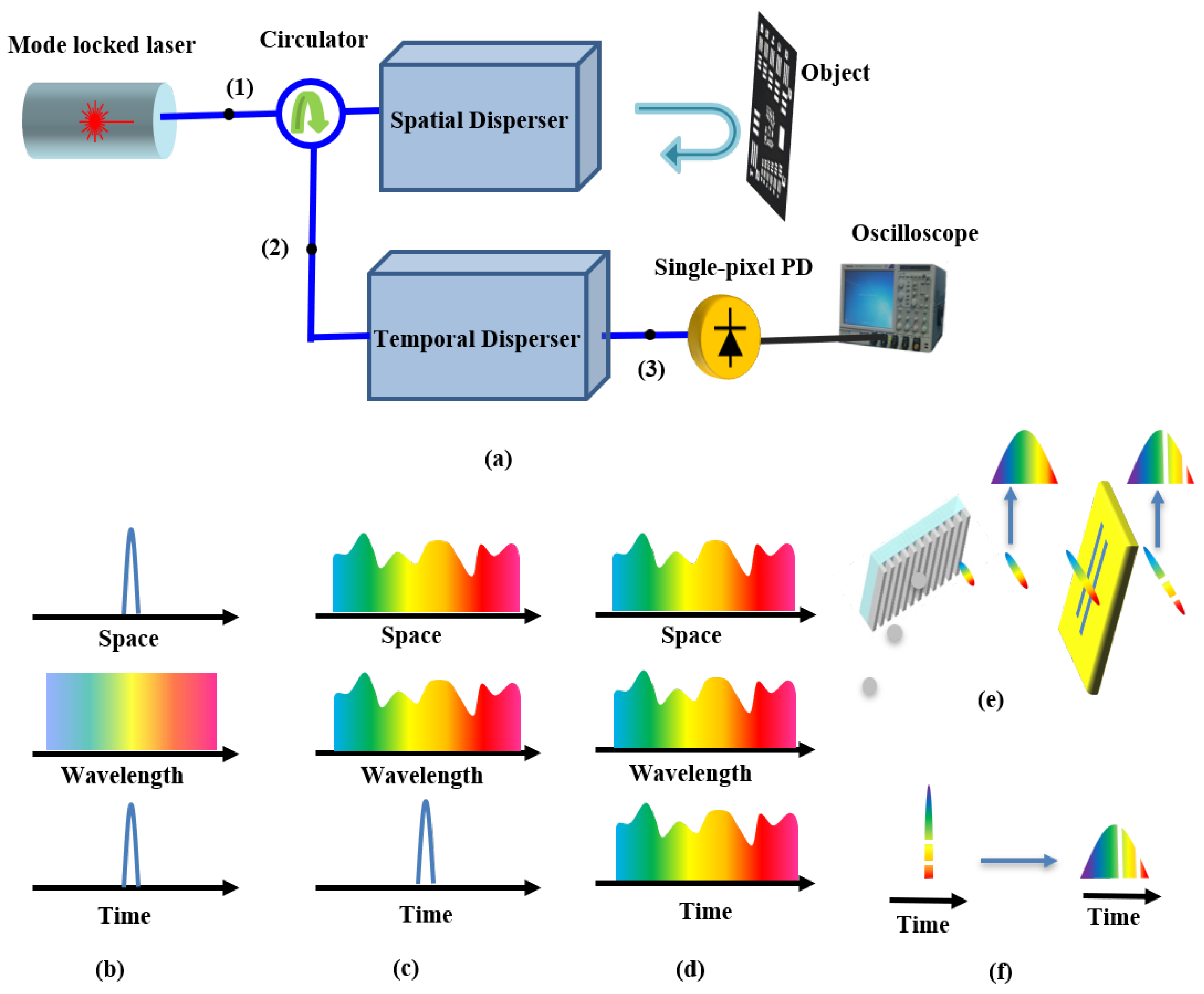
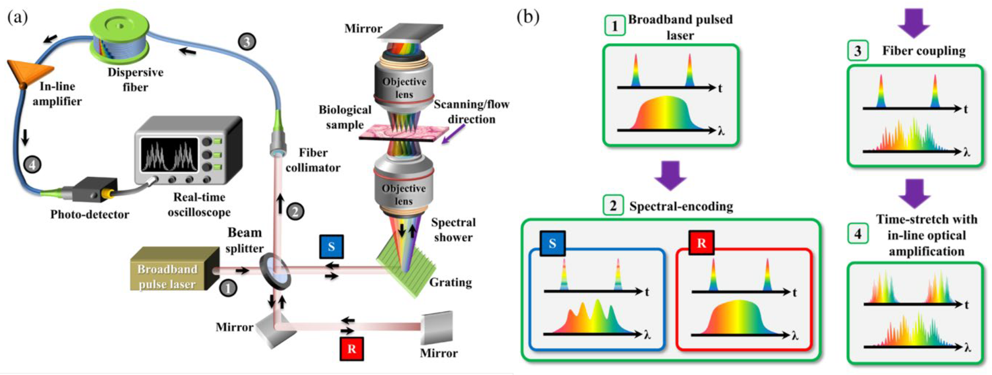
The schematic of the ultrafast PTS imaging system is shown in Figure 1a. The incident broadband-pulsed light from a mode-locked laser is emitted into the imaging object via a spatial disperser, where space-to-wavelength conversion is obtained. The light information in space, wavelength, and time domain at point (1) is shown in Figure 1b. Different spectrum of light is illuminated to the corresponding spatial coordinates of the imaging object. The reflected light returned to the same spatial disperser and was combined into a single pulse. The shape of the light pulse, which shows the imaging coordinates of the object, is encoded into wavelength. The light information in space, wavelength, and time domain at point (2) are shown in Figure 1c. Then the light pulse propagates the temporal disperser, where wavelength-to-time conversion is acquired. Usually, due to the nonlinear effect of the temporal disperser, the femtosecond pulse is stretched to nanoseconds level. After the wavelength-to-time conversion, the shape of the light pulse in the wavelength domain is mapped to the time domain based on the one-to-one linear mapping. The light information in space, wavelength, and time domain at point (3) are shown in Figure 1d. Figure 1e shows the light pulse change in the spectral domain. Light from a pulsed broadband light source passes through the grating and then scatters into space with angular dispersion achieved. The pulses propagate the two-bar sample, and the spectral shape is obtained. Figure 1f shows the light pulses change in the time domain. The femtosecond pulse is stretched into nanosecond pulse after passing through the temporal dispersive devices. Then, space-to-wavelength-to-time one-to-one-to-one conversion is achieved [21,29]. Afterward, the femtosecond pulse is stretched into a 1D temporal profile data for a single pixel PD detection. The data then are acquired and displayed by the oscilloscope. The pulse is repeated for imaging acquisition, and the frame rate of the PTS imaging system equals the repetition rate of mode-locked laser.
Compared to imaging systems using charged coupled devices (CCD) or complementary metal oxide semiconductors (CMOS) [82,83], it removes the limitation of low speed of image acquisition and low readout speed. Additionally, it prevents the drawback of a low signal-to-noise ratio (SNR) at a high frame rate [84,85,86]. Compared to the other imaging systems using a beam-scanning method based on single-pixel PD, it avoids the low imaging frame rate that inherently exists in the scanning methods [87] while at the same time maintaining the same level of SNR. This PTS-based imaging system is confirmed to have the merits of ultrafast imaging speed that conquers the traditional trade-off limitation between imaging speed and SNR.
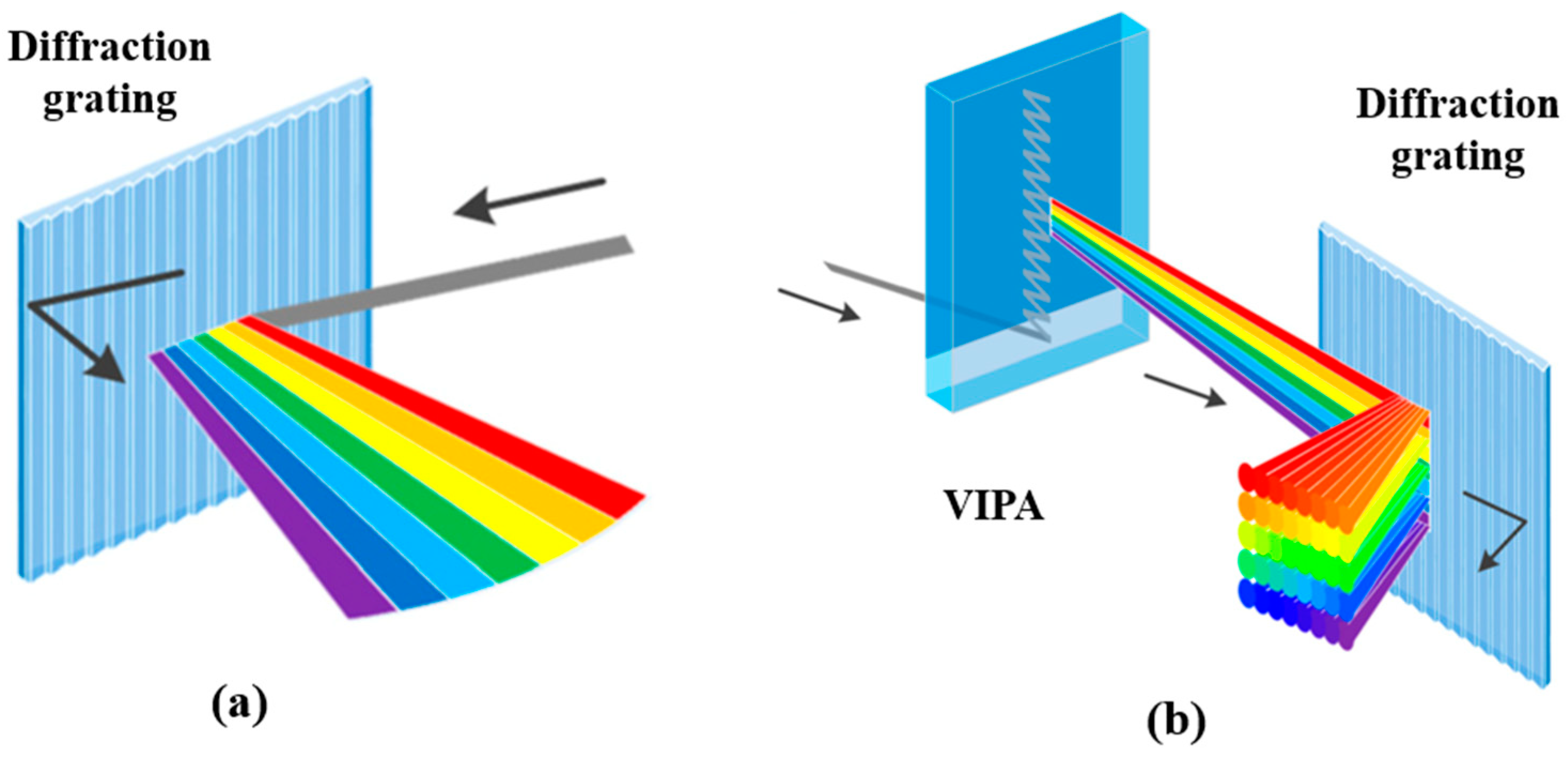
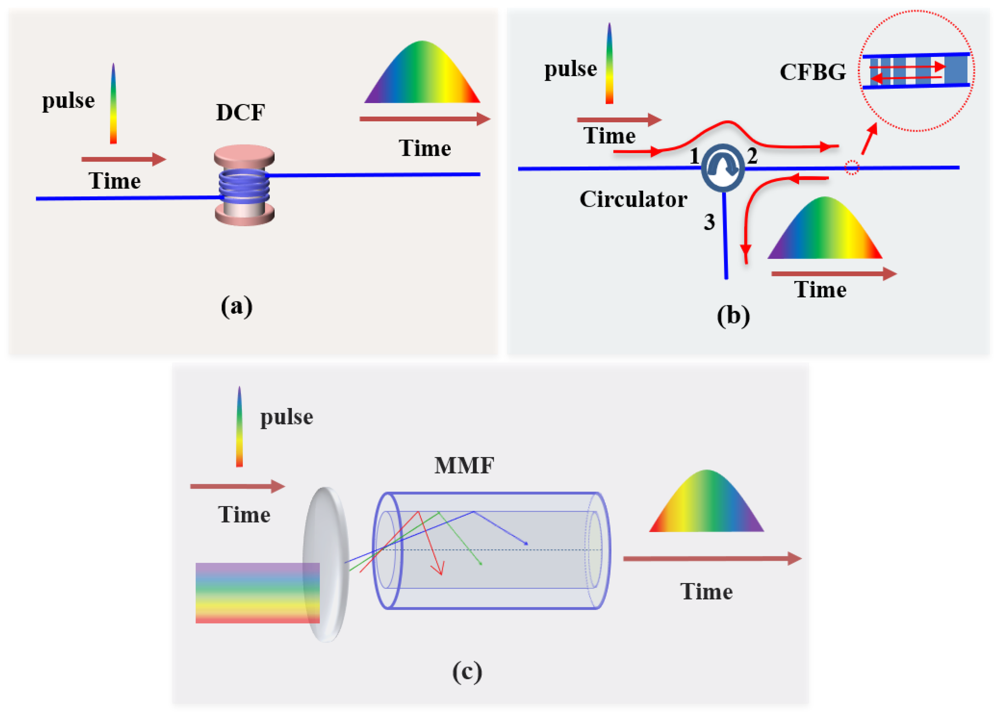
The key elements of PTS imaging systems are spatial disperser [88,89] and temporal disperser [3,59]. A spatial disperser is used to enable wavelength-to-space conversion at the imaging coordinates plane; thus, the light of different wavelengths will be emitted to different physical positions. Figure 2a illustrates the 1D spatial dispersion using a diffraction grating to produce a 1D rainbow light beam. Figure 2b shows the 2D spatial dispersion based on a pair of virtually imaged phased arrays (VIPA) [90,91,92] and a diffraction grating [93]. The VIPA has a structure of etalon, which has one surface with a high-reflectivity coating and another with partial-reflectivity. The 2D spatial dispersion process is shown in Figure 2b. VIPA generates 1D continuous multiple wavelengths of the light beam and further unfolded by the diffraction grating, and thus a 2D rainbow light beam is generated. A temporal disperser is used to obtain the wavelength-to-time conversion—a process called PTS or dispersive Fourier transformation (DFT) [94,95]. This process is based on the light of different wavelengths traveling in the medium at different speeds; upon certain propagating length, the light of varied wavelengths will reach the garget at different times. PTS or DFT enables real-time imaging measurement at ultrafast speed. Normally linear and large (more than 100 ps/nm) temporal dispersion is required for PTS or DFT process, and the light bandwidth for imaging application is at least 10 nm with a center wavelength of around 1550 nm [28]. Figure 3a shows the temporal disperser based on dispersive compensating fiber (DCF) [21], which provides chromatic dispersion and normally has a large linear temporal dispersion (more than 100 ps/nm). Figure 3b describes another way to perform temporal dispersion based on a chirped fiber Bragg grating (CFBG), which provides a wavelength-dependent time delay [96,97]. The pulsed incident light passes through port 1 and then port 2 of the circulator, and then the light reaches the CFBG and returns into port 2 by the reflection of CFBG, the light then goes through the circulator form port 2 to port 3. Figure 3c reveals the realization of temporal dispersion using multimode fiber (MMF) based on large chromo-modal dispersion [98]. Additionally, excess temporal dispersion should be avoided as this will lead to the 1D data stream being overlapped among the adjacent laser time-stretched pulses.
3. Applications
The recent development of PTS imaging systems are mainly in four categories: first, PTS imaging systems combined with shorter wavelength bands for better imaging resolutions and rich applications [68,69,70,71,72,73]; second, PTS imaging systems with faster speed [21,22,26,27,28,29,57,58,74,79]; third, PTS imaging systems combined with data compression [11,12,13,14,15,16,17,18,75,76,77,78]; and the last, PTS imaging systems combined with deep learning for target classification [23,24,25,32,66].
3.1. Shorter Wavelength Band for PTS Imaging
In the first category, the shorter wavelength band in the PTS imaging method results in better spatial resolution in principle. The “short” stands for wavelength spans from visible to near IR. Three examples will be displayed in this part, first is the 932 nm laser generation and dual color imaging with customer-designed light source revision; the second is the 710 nm imaging using special customer-designed device-FACED with the spatial dispersive device revision; last is the 1064 nm phase imaging with the systematic structure revision.
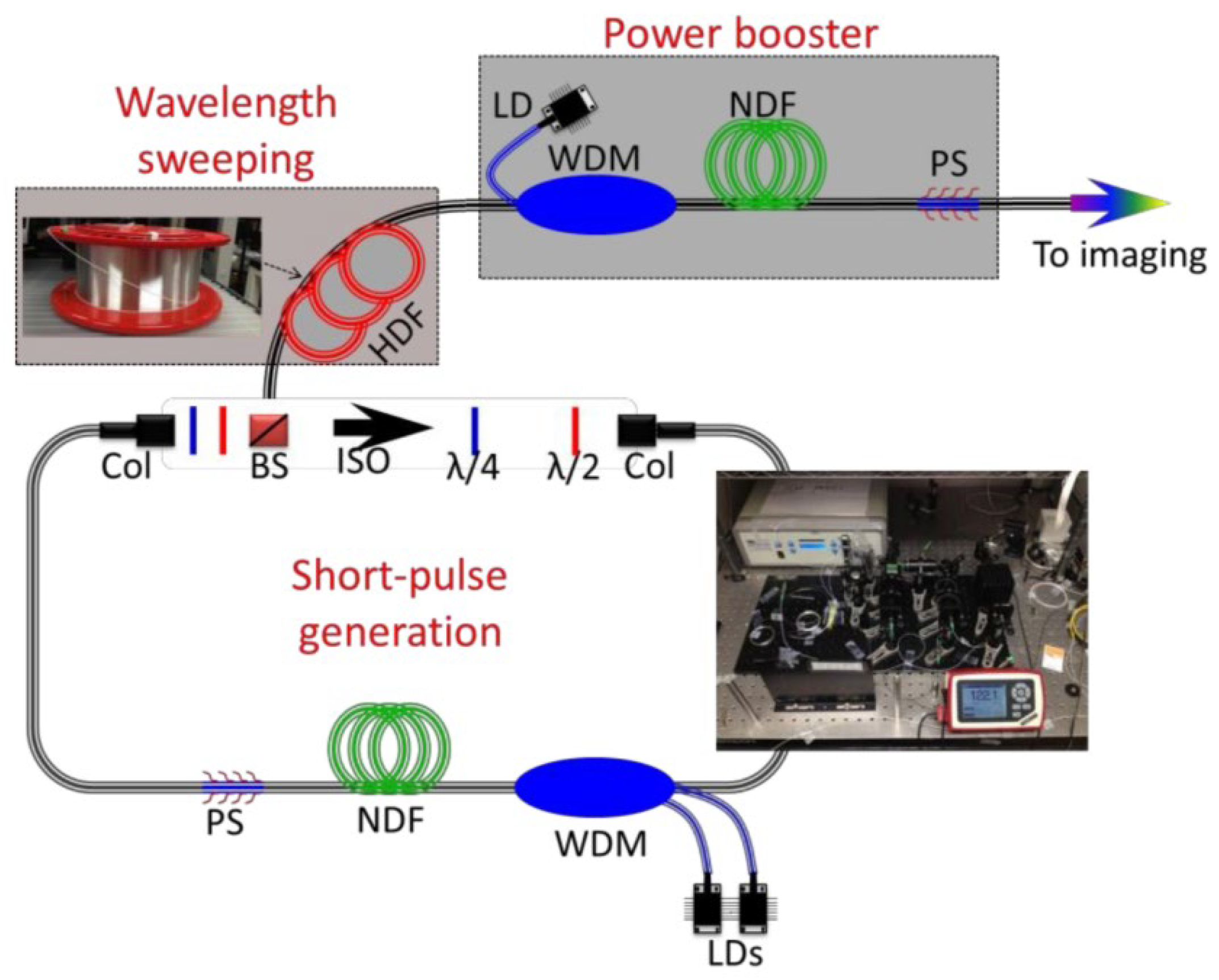
The first example of the PTS imaging system uses a 932 nm laser with the assistance of a new highly dispersive fiber (HDF), enabling MHz optical imaging [68]. The configuration of the swept source at 932 nm is shown in Figure 4. The configuration of a swept source contains three main elements: short pulse generation, wavelength sweeping, and power booster. Nonlinear polarization rotation mode-locking is applied in the fiber ring resonator, where a short pulse is generated. A 20-m double-cladding neodymium-doped fiber (NDF) is employed as the gain medium to boost laser output power. The wavelength sweeping is realized by using a custom-made HDF operating at a wavelength band of 800–1100 nm.
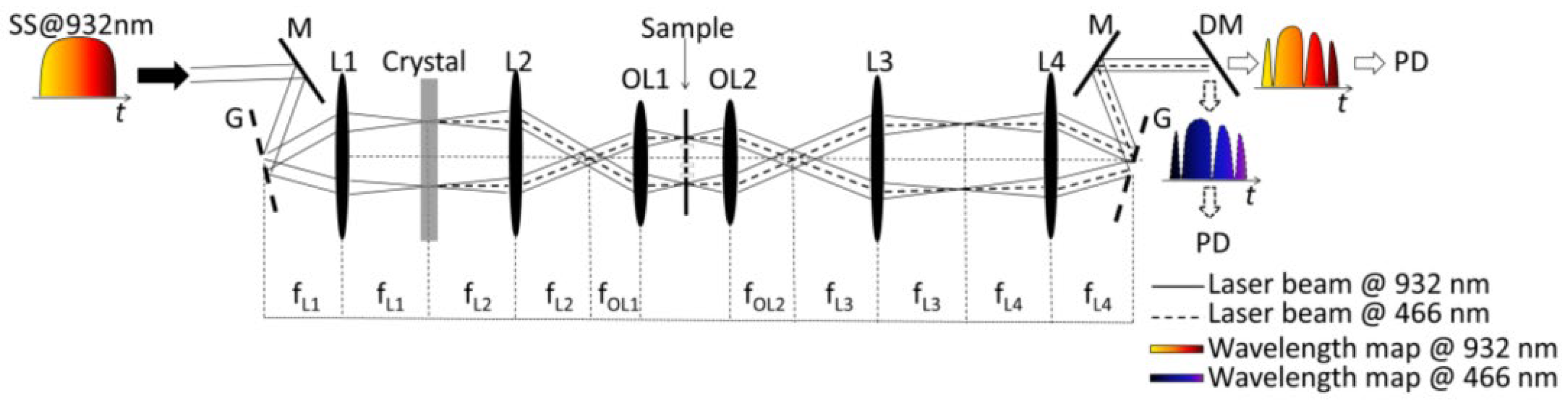
The schematic diagram of the ultrafast dual-color imaging system based on HNF is shown in Figure 5. The wavelength-swept source has a center wavelength of 932 nm and a bandwidth of 7.2 nm at full width at half maximum. Light from the swept source is spatially dispersed by the diffractive grating, which has a groove density of 600 mm. A nonlinear BBO crystal is placed at the Fourier plane of L1 for second-harmonic generation (SHG) in order to demonstrate dual-color imaging at visible and near-infrared (NIR) wavelength bands. After the BBO crystal, 932 nm and 466 nm co-existed. After light illumination, light propagation, and light detection after wavelength separating using a dichroic mirror, the dual-color light information is processed to recover imaging.
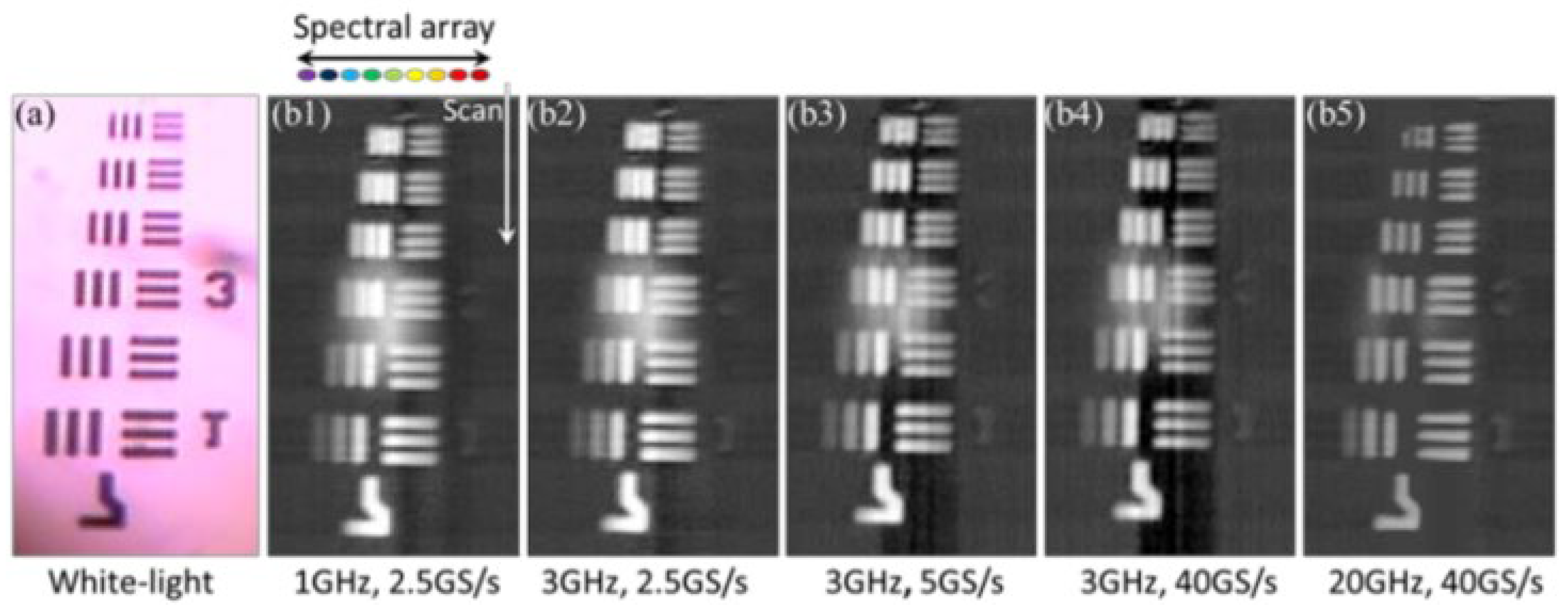
To demonstrate the capability of the PTS imaging system, a 7.6 MHz line-scan imaging is performed. The white-light imaging of the USAF-1951 resolution target is shown in Figure 6a. Figure 6b describes the line scanning result at varied bandwidths and sampling rates (from 1 GHz, 2.5 GS/s to 20 GHz, 40 GS/s).
The second example of the PTS imaging system is called free-space angular-chirp-enhanced delay (FACED) [70]. FACED generated high temporal dispersion and low intrinsic loss at a visible wavelength (~710 nm). FACED also enabled fluorescence and colorized time-stretch imaging while at the same time having the benefit of low intrinsic loss.
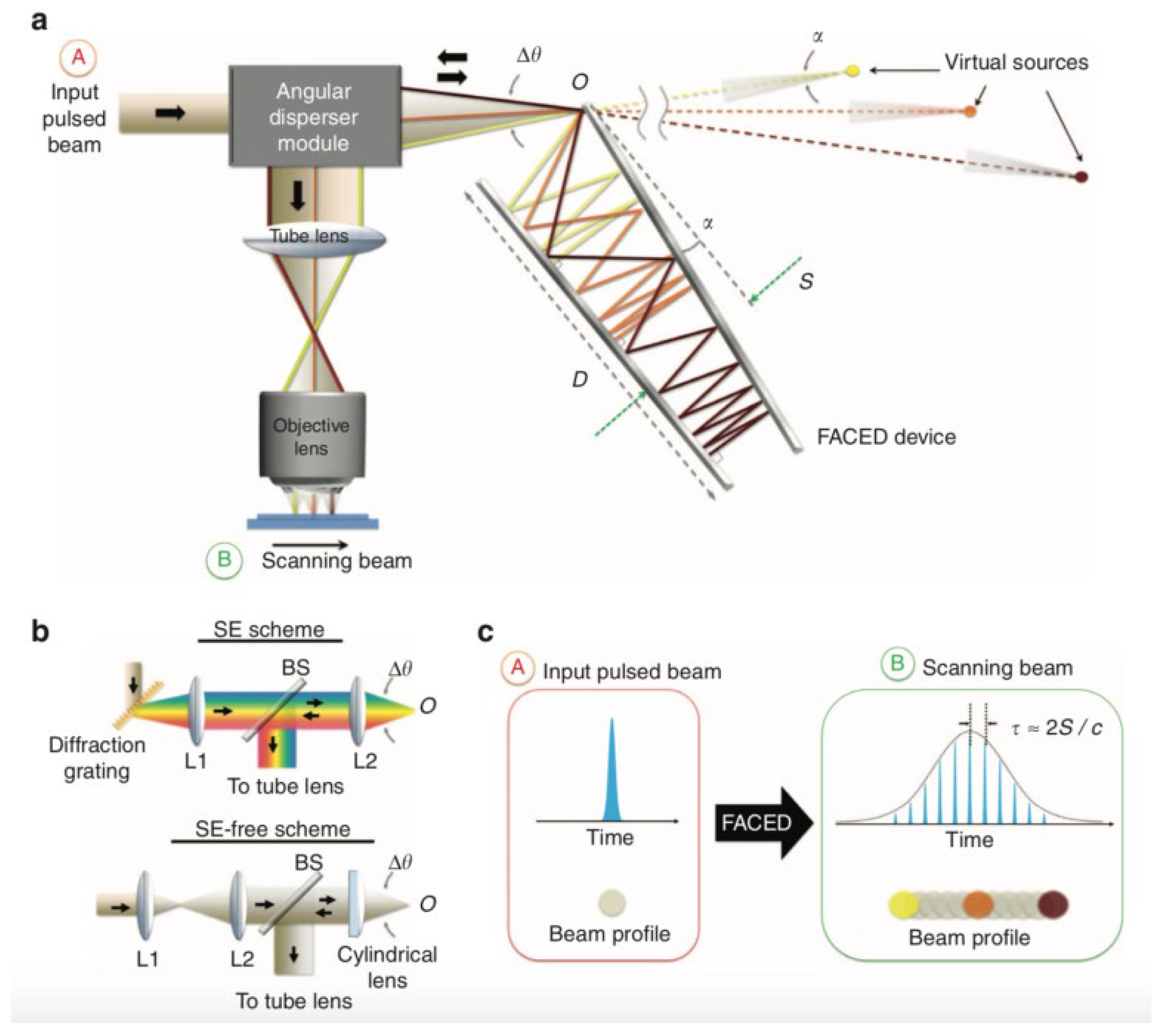
Figure 7 shows the working principle of FACED. A pair of highly reflective plane mirrors placed at a distance of S with a minute mirror misalignment angle α (typically 10−3 rad) is employed to realize the working principle of time-stretch at visible wavelength. The pulse is propagated and stretched in free space within the space between two reflective plane mirrors, shown in Figure 7a. The pulse stretching resulted from the misalignment of two mirrors, which generated ample and configurable time delay among the cardinal rays. To stretch the pulse within the two mirrors, the pulse is demanded to focus at the entrance point of the FACED device, O. This results from the application of an angular disperser module. The scheme of an angular disperser module is depicted in Figure 7b. In the spectral encoding (SE) scheme, a diffraction grating is used as an angular disperser. In the SE-free scheme, a focusing lens is applied as the angular disperser. The main concept of FACED is shown in Figure 7c. It not only can perform pulse stretching in the temporal domain but also can transfer an input simultaneous pulse beam into a time-encoded serial scanned beam in space.
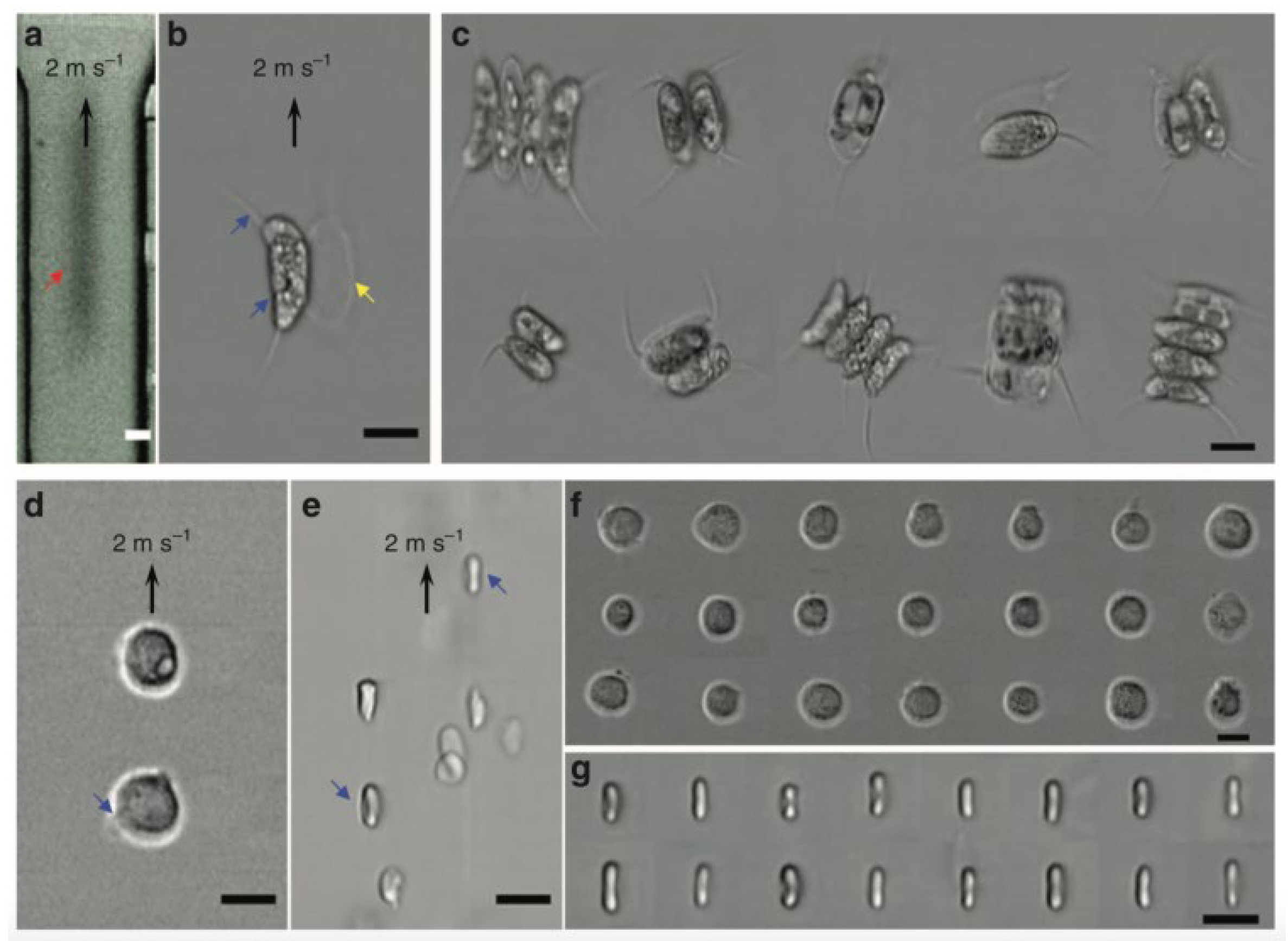
The demonstration of FACED-based PTS microscopy working on SE scheme in an ultrafast microfluidic flow with a speed of 2 m/s at a line-scan rate of 80 MHz. The imaging results are shown in Figure 8. In comparison with the images detected by high-speed CMOS camera (15,000 fps, Figure 8a), FACED-based PTS microscopy captured images of Scenedesmus acutus cells (Figure 8b,c), monocytic leukemia cells (THP-1; Figure 8d,f), and human red blood cells (RBSs; Figure 8e,g), are blur-free and at the same time have higher resolution, showing the fine subcellular features. For example, the blebs of the THP-1 and the biconcave shapes of the RBCs are displayed in Figure 8d,e.
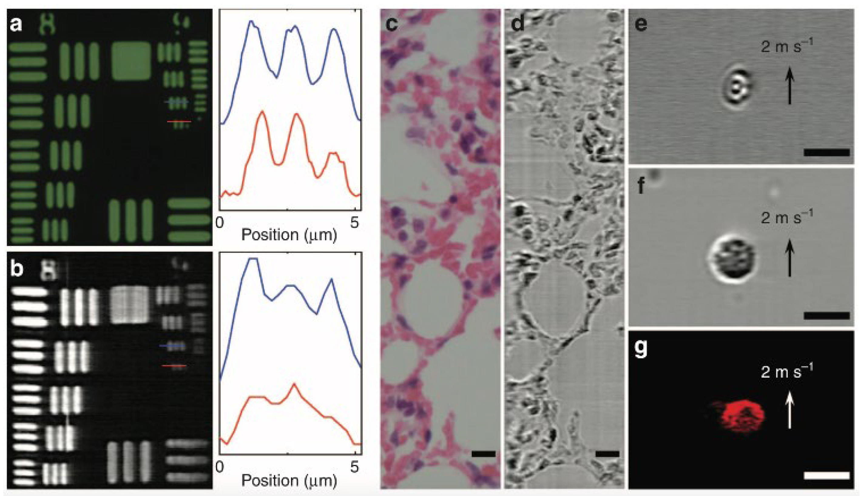
Figure 9 shows the FACED-based microscopy working on the SE-free scheme. The bright-field and FACED-based microscopy images on the smallest element of group 9 of resolution target USAF-1951 are shown in Figure 9a,b, respectively. The FACED-based image has a slightly lower resolution. The slightly lower resolution of the FACED images is owing to the smaller number of scanned spots, and this resolution can be improved by adjusting both the mirror misalignment angle and the input cone angle. The static sample of a hematoxylin-and-eosin (H&E)-stained lung tissue section is also applied for bright-field (Figure 9c) and FACED-based microscopy (Figure 9d) imaging. An ultrafast microfluidic flow at 2 m/s of RBCs and peripheral blood mononuclear cells (PBMCs) are illustrated in Figure 9e,f, respectively. Additionally, the fluorescence FACED-based microscopy working on the SE-free scheme with a line-scan rate of 8 MHz is demonstrated using a 10 μm fluorescent bead in the ultrafast microfluidic flow at 2 m/s. The result is shown in Figure 9g.
The third example is interferometric PTS (IPTS)-based microscopy for ultrafast quantitative cellular and tissue imaging at 1 μm wavelength band [72]. IPTS-based microscopy could overcome the traditional imaging speed limitation of the quantitative phase imaging method. The line-scan rate of IPTS-based microscopy could be as high as 20 MHz, and the ultrafast flowing cells with a flow speed of 8 m/s are several orders of magnitude higher than conventional quantitative phase imaging.
The overall schematic of the IPTS-based microscopy is illustrated in Figure 10a. A laser source with a center wavelength of 1064 nm, a bandwidth of 10 nm, and a repetition rate of 26.3 MHz or bandwidth of 60 nm and a repetition rate of 20 MHz is provided as the microscope source. The pulsed laser is split into two beams through a beam splitter. One beam is treated as the signal beam passing through the biomedical samples. The other beam is regarded as the reference beam, reflected by mirrors. Then the two beams combined into one via the same beam splitter and propagated through the dispersive fiber. After pulse amplification and detection, the pulse information is ready for processing. Figure 10b shows the waveforms of temporal and spectral domains of different stages.
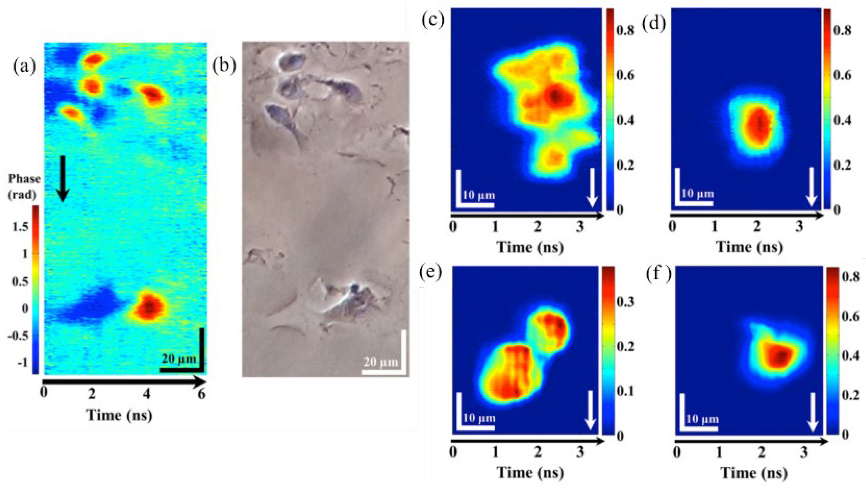
The result of fixed epithelial cells by IPTS-based microscopy at a line-scan rate of 1 MHz and conventional phase contrast microscopy is described in Figure 11a,b, respectively. When the ultrafast flowing cells with a flow speed of 8 m/s and 0.4 m/s, a cluster and single HeLa cells and normal hepatocyte cells (MIHA) are captured by the IPTS-based microscopy, which is shown in Figure 11c,d and Figure 11e,f, respectively. The ultrafast flow speed (8 m/s) corresponding to an imaging throughput as high as 80,000 cells/s. Thus, this IPTS-based microscopy is proved to be an ultrafast quantitative phase imaging.
3.2. Fast Speed for PTS Imaging
The second category describes the world’s fastest frame rate based on PTS microscopy. The frame rate of PTS microscopy equals the repetition rate of the pulsed laser.
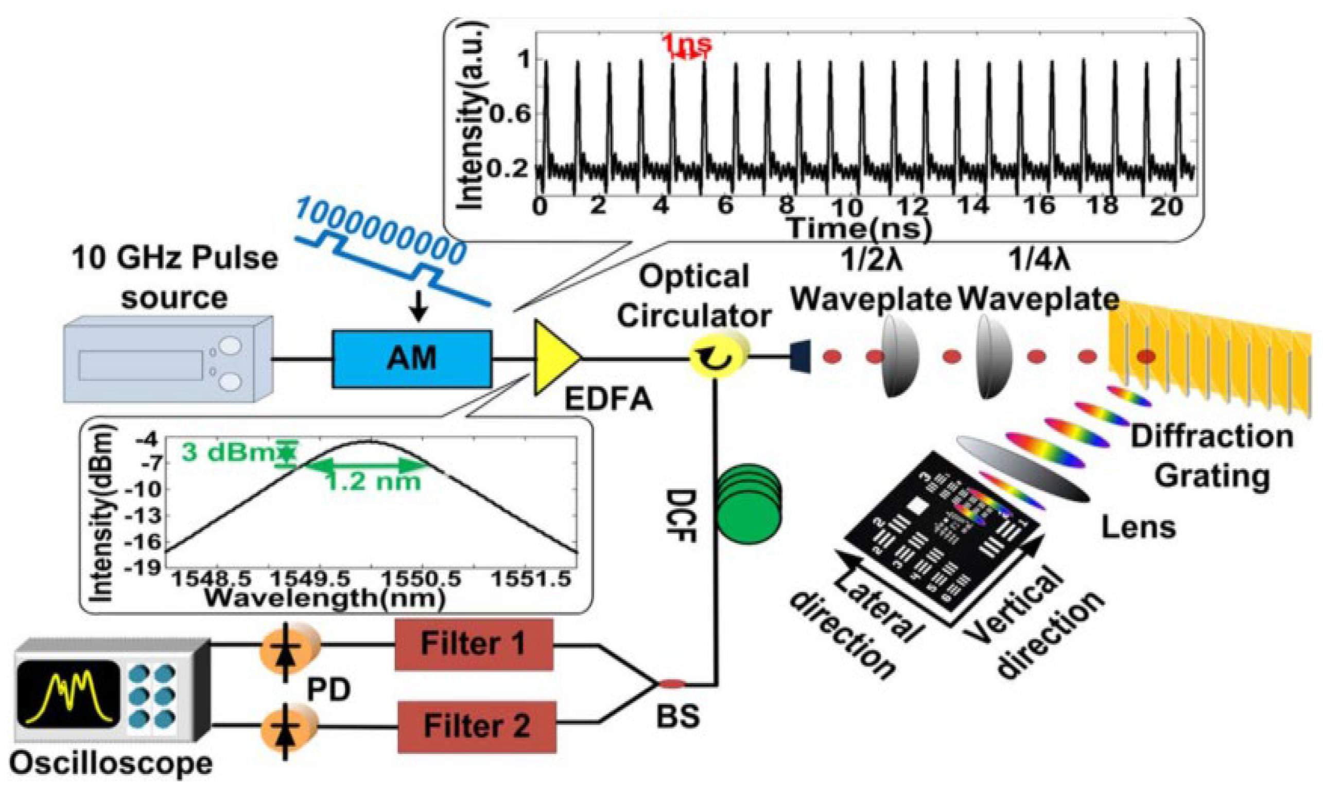
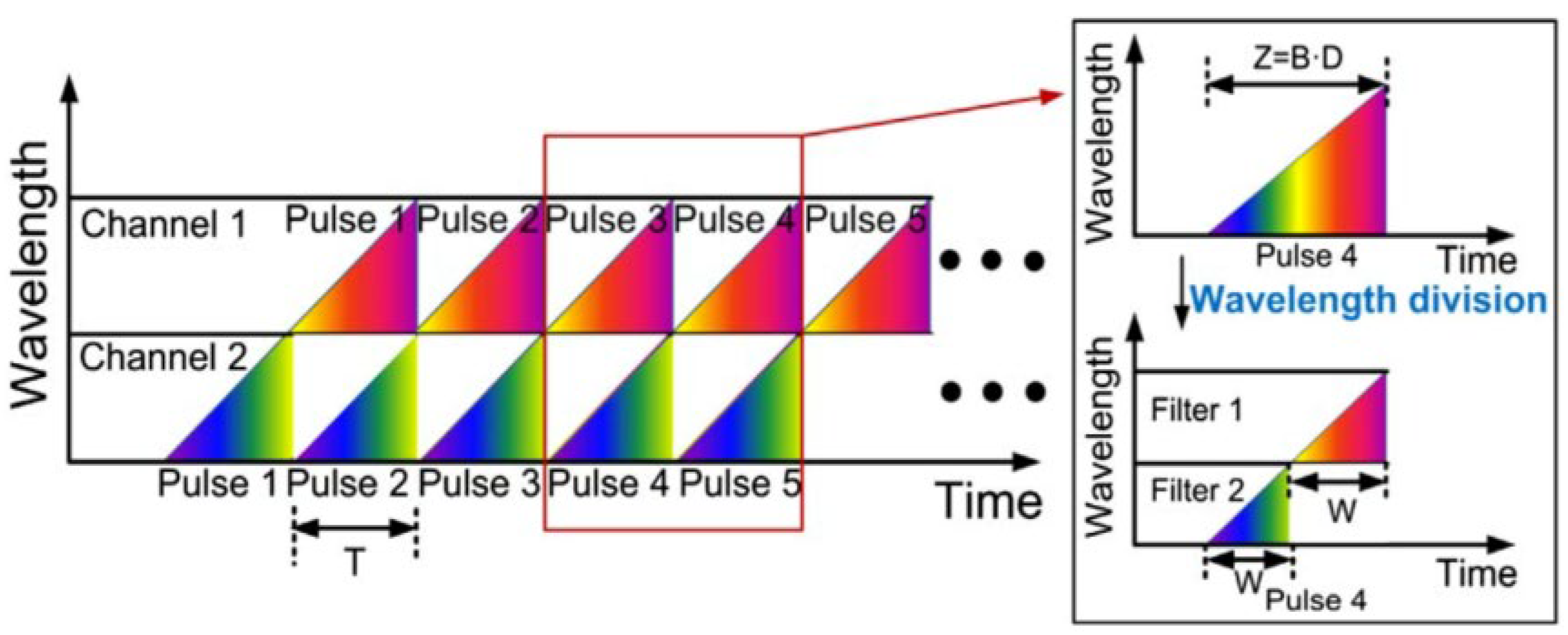
In this category, a pulsed laser source with a repetition rate of 10 GHz, a center wavelength of 1549.2 nm, a 3 dB bandwidth of 1.2 nm, and a pulse width of 2 ps is employed [74]. The schematic of the superfast PTS imaging system is shown in Figure 12. The frame rate, in theory, can be as high as 10 Gfps. Due to the dispersion limitation (a dispersion of 1377 ps/nm), a gated Mach–Zehnder amplitude modulator is utilized to reduce the repetition rate to 1 GHz. The pulse propagated through the diffraction grating and sample and reflected for data detection with the same path back. The high temporal dispersion leads to pulse overlapping; thus, a wavelength division technique is utilized, which can overcome the trade-off between a high frame rate and spatial resolution. In practice, the temporal signal is equally split into two channels by varied wavelength-band filters at the receiver end.
The principle of the wavelength division technique is shown in Figure 13. The dispersed pulses are linearly chirped, and adjacent pulses overlap in the time domain. As shown in Figure 13, T stands for the period of the pulse laser, Z is the temporal width of the dispersed whole pulse, B is the spectral bandwidth of the optical pulse, D is the group velocity dispersion (GVD), and W is the width of pulse filtered from each channel. Then the two channels without temporal overlap are detected by high-speed PD, and then further data processing is applied to recover the image.
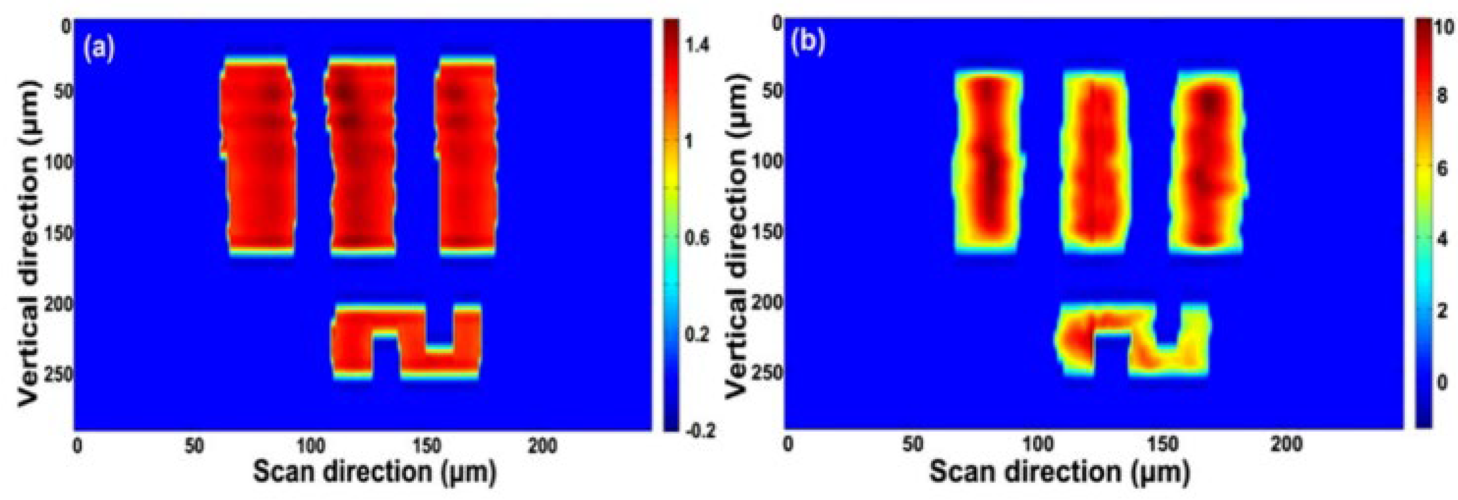
A USAF-1951 resolution target is utilized for imaging at element 2, group 4, with a line width of 28 μm. The same 2D image is reconstructed at a 100 MHz scan rate (Figure 14a) and 1 GHz scan rate (Figure 14b); the quality of the image does not degrade with the increasing line scan rate. The state-of-art of this demonstration validates the capability of the PTS-based 1 GHz microscopy with wavelength-division technique.
3.3. Data Compression for PTS Imaging
The third category describes the data compression techniques combined with PTS-based microscopy. The high amount of real-time digital data generated by the equipment leads to an unintended consequence of extremely high throughput imaging acquisition, which brings a heavy burden for the data acquisition and, following data processing, sets the barrier to real-time imaging. Here, two techniques will be discussed in this category.
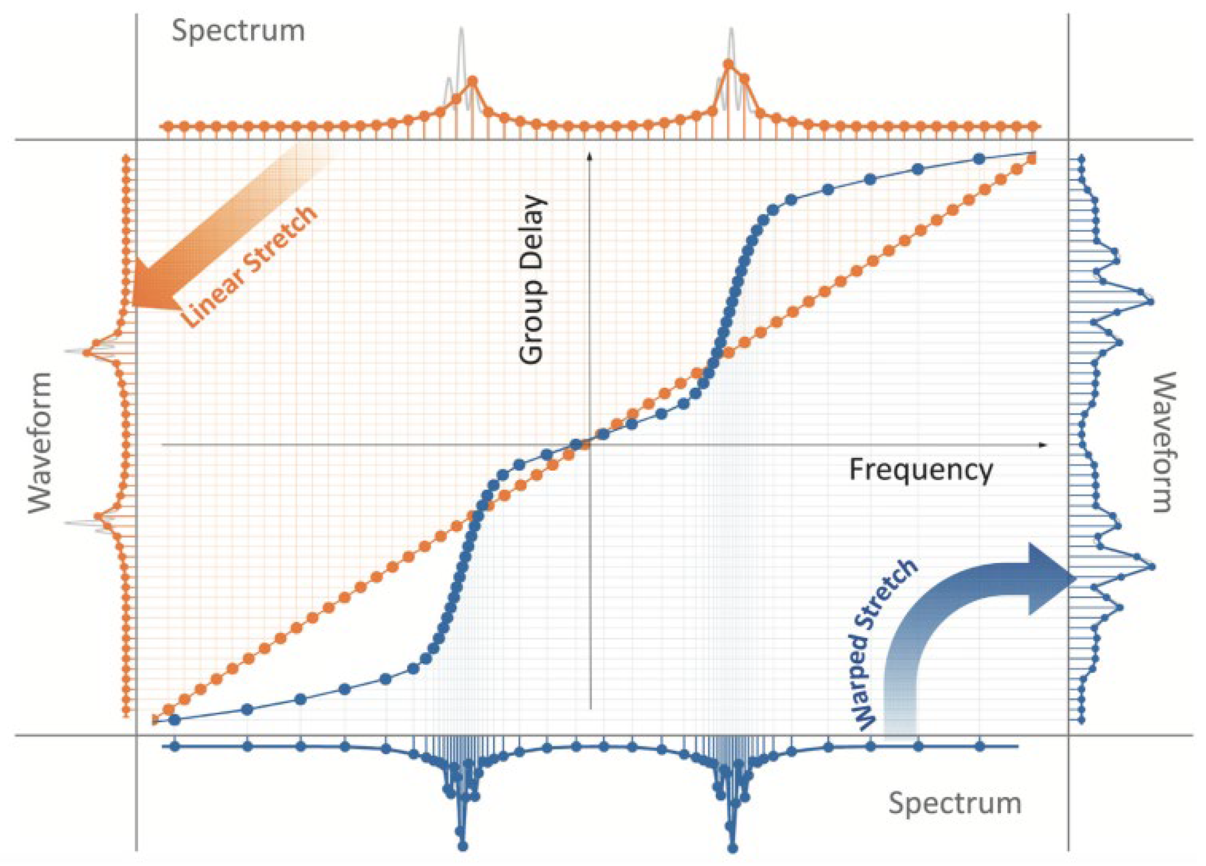
The first technique is called anamorphic time stretch (AST) or warped time stretch [13,14,15,77], which is realized via nonlinear GVD. AST reshapes the spectro-temporal profile of optical signals so that the signal envelope’s time-bandwidth product is compressed. The compression is obtained from the nonlinear time-stretch or nonlinear spectral-to-time mapping.
Figure 15 shows the linear and AST dispersive Fourier transforms [14]. Orange points depict the linear time stretch between spectrum and time. The constant straight slope line reveals the linear GVD. The spectral components of the pulse train are linearly distributed in time, even in the silent time zone, which increases the amount of invalid data. In a linear time stretch scheme, the spectrum of the pulse and the waveform are uniform with the same sampling resolution. In contrast, blue points show a nonlinear GVD that varied GVDs over the spectrum can stretch the spectrum nonlinearly. With nonlinear GVD, regions of the spectrum are stretched more than others, leading to the nonlinear mapping between the spectrum and waveform. If the sparsity of the spectrum of the under-testing imaging is known, thus a dense spectral zone with large GVD while a silent spectral zone with small GVD could increase the imaging resolution and, at the same time, maintains the same amount of data.
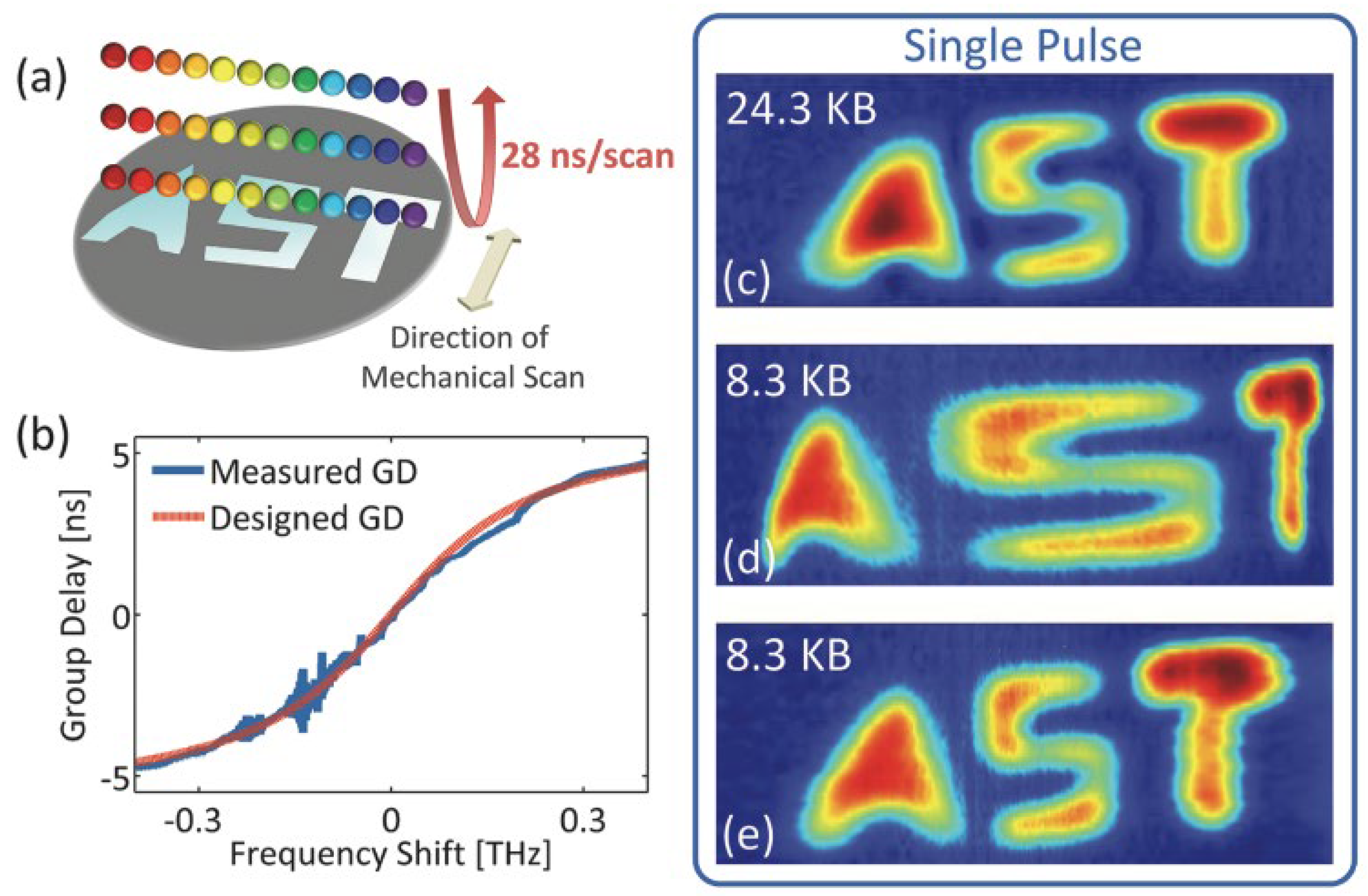
The experimental result of the PTS-based imaging system with nonlinear time stretch over the spectral bandwidth is shown in Figure 16. Figure 16a illustrates how the test sample (with a width of 5 cm) reflected one-dimensional rainbow illumination pulses (with a repetition rate of 36 MHz). Figure 16b states the shape of the nonlinear time stretch between the GVDs and spectral components. It is designed and performed by a custom chirped fiber Bragg grating (CFBG) with a nonlinear group delay profile. If a high linear dispersion (same as the warped stretch at the center frequency) is linearly distributed among all the spectral components, the recovered image size is 24.3 KB in Figure 16c. With the nonlinear time stretch of the waveform owing to the utility of CFBG, the reconstructed imaging is shown in Figure 16d with an image size of 8.3 KB and an obvious warping effect in the letter “S”. With the assistance of the unwarping algorithm, the uniform image with a size of 8.3 KB is reconstructed and illustrated in Figure 16e. It reveals a data compression ratio of 34% and maintains the same imaging resolution.
The second technique is named compressive sensing (CS) [16,17,18,73,99,100,101,102]. Due to the sparsity of the desired imaging, the extensively used CS method can reduce the number of measurements and offers a high-efficient data acquisition process. For example, in reference [10], in a PTS-based imaging system, a laser with a repetition rate of 50 MHz and an acquisition rate of 50 MHz is obtained via CS. Without CS, the traditional acquisition rate is much higher. For example, a laser with the same repetition rate of 50 MHz and an acquisition rate of 100 GHz is applied [26] in a PTS-based imaging system. Hence, the utilization of CS can greatly reduce the acquisition rate. With the combination of CS and PTS-based imaging, the data information can be compressed to a high level [13]. The extensively utilized CS technique uses random patterns to mix the imaging sampling and then reconstruct the image based on its algorithms.
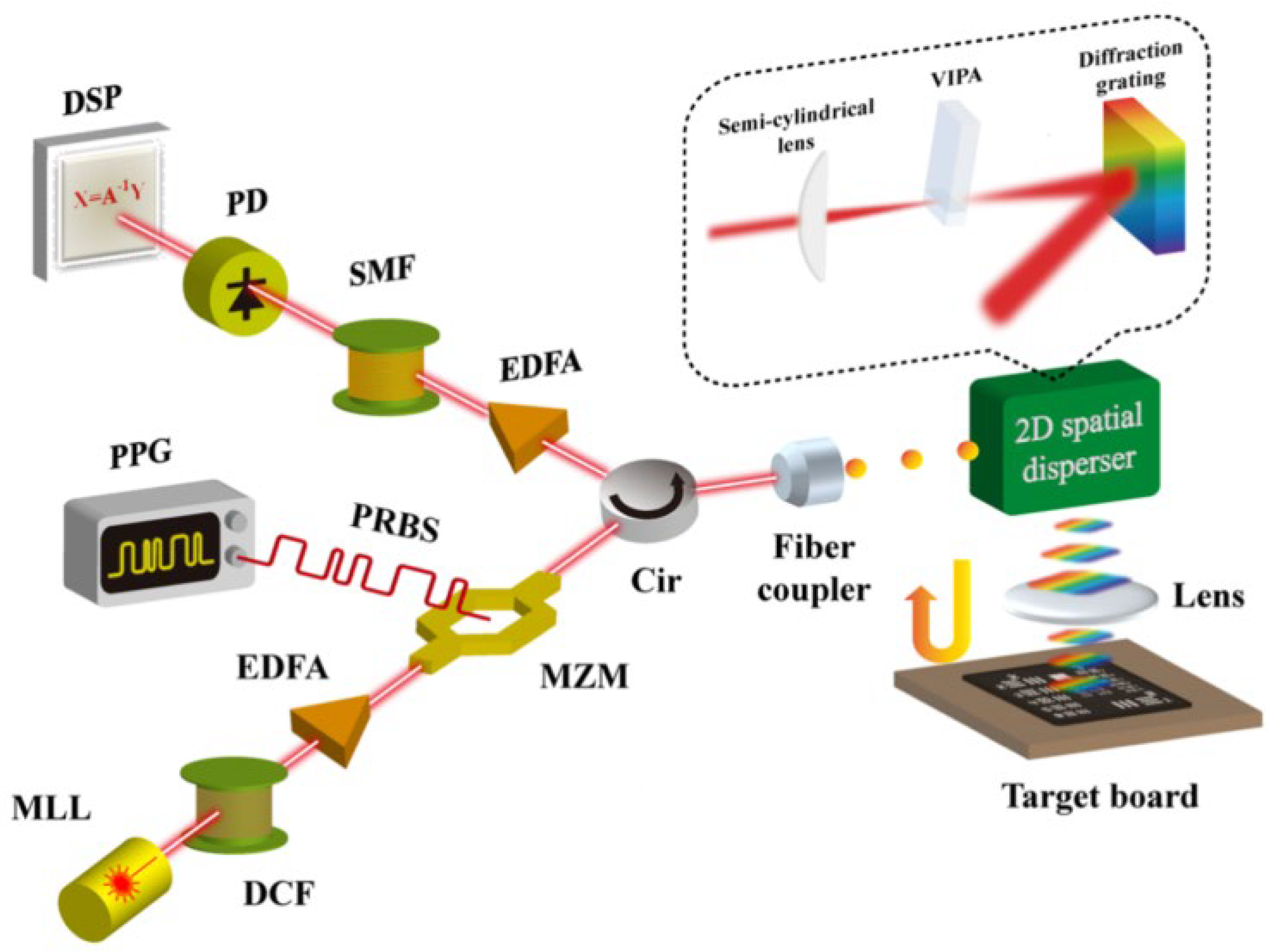
The schematic of the combination of the CS technique and PTS-based imaging system is shown in Figure 17 [13]. Compared to classical PTS-based imaging systems, the CS and PTS-based imaging systems added a pulse pattern generator (PPG) that generated pseudo-random binary sequences (PRBSs). The RPBSs mixed the pulse signal when the light pulses propagated through the Mach-Zehnder modulator (MZM). The light pulses, reached the target and were detected by PD for imaging reconstruction based on CS algorithms.
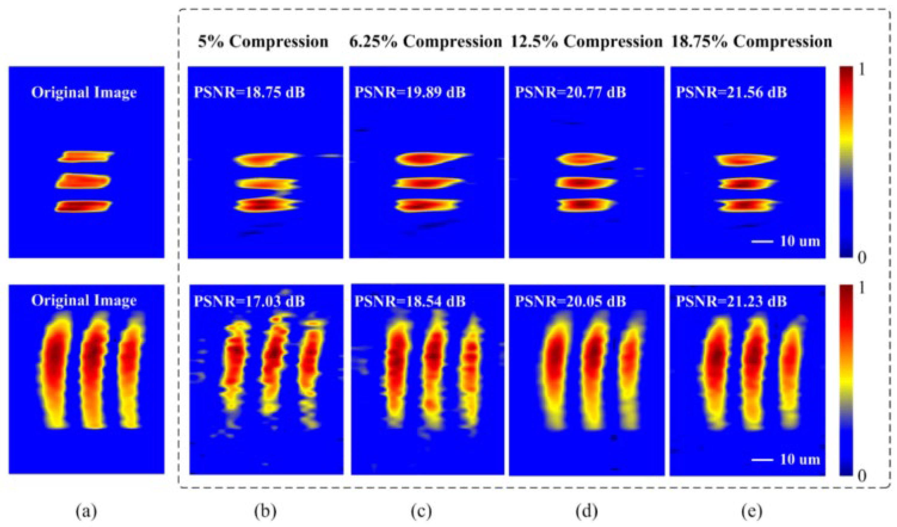
Reconstructed images are displayed in Figure 18. Captured 2D images without CS are shown in Figure 18a. Figure 18b–e reveals the reconstructed images at different compression ratios of 5%, 6.25%, 12.5%, and 18.75%, respectively. The imaging recovery precision of varied compression ratio is evaluated by the peak-SNR (PSNR) of the reconstructed images, shown in Figure 18. This technique can achieve a data compression ratio of 5% with fair image recovery precision.
3.4. Deep Learning for PTS Imaging
The last category falls into the combination of PTS-based imaging systems with deep learning for classification [23,24,25]. PTS-based imaging can generate a large number of images; hence, high throughputs of images of the imaging system are compatible with deep learning methods for classification.
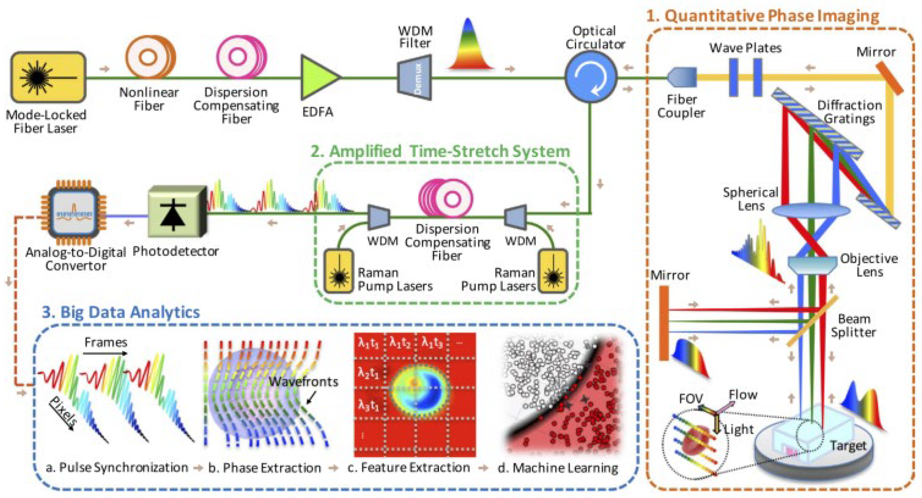
A sample of PTS-based quantitative phase imaging (QPI) with deep learning is stated in this category. The schematic of the PTS-based QPI and analytics system is shown in Figure 19 [23]. The system has three key parts: first (in the yellow box), QPI based on Michelson structure enables blur-free imaging with a high throughput of 100,000 cells/s; second (in the green box), amplified time-stretch system provides not only wavelength-to-time one-to-one mapping but also optical power amplification for the following optical pulse detection; last (in the blue box), the big data analytics offers images reconstruction, images analysis and images classification based on machine learning method.
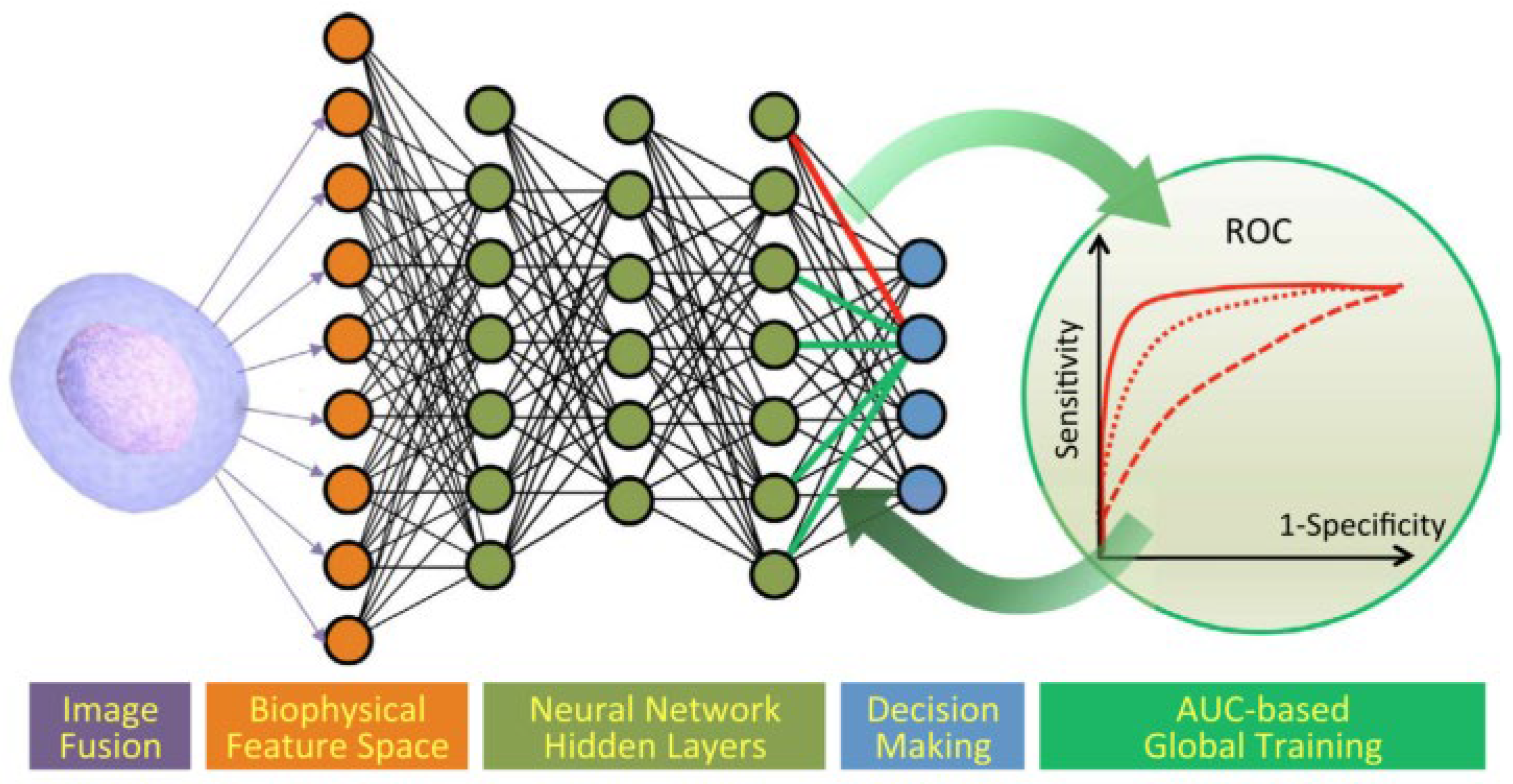
The principle of the feedforward neural network learning model pipeline is shown in Figure 20 [23]. First, the images are fused, and the major features from the quantitative images are extracted. Then, the biophysical feature space is fed into the neural network, which has the purpose of decision-making. This machine learning model is globally trained with the objective of improving receiver operating characteristics (ROC). The learning algorithm maximizes the area under the ROC curve (AUC). Then, the training network results in a robust and repeatable classifier, which improves sensitivity and specification. A successful demonstration of cell classification of white blood T-cells, colon cancer cells, and lipid-accumulating algal strains are obtained.
4. Discussion
The future trends of optical time-stretch imaging emphasize more intelligence, more integration, and more bandwidth extension.
With the emerging development of ChatGPT [103], artificial intelligence and deep learning have been employed in varied applications. Optical time-stretch imaging is inherently compatible with a variety of imaging processing algorithms, which has the benefit of easy access to intelligent imaging processing, such as trained deep learning for imaging recognition and classification. Previously, imaging classification was already utilized [23]. With the development of hashrate, intelligent time-stretch imaging processing will be faster and more precise.
Conventionally, nearly all illustrations of optical time-stretch imaging are performed using an oscilloscope for real-time display, ADC for signal sampling, and then offline signal processing. Few demonstrations show the integration of hardware to handle the high throughput. That is to say, advanced computational techniques are required to be embedded in the hardware, such as in FPGA, to process the streaming mass data. This is so-called computational integration. Another type of integration is systematic integration, which is the miniaturization of all-optical time-stretch imaging systems thanks to the Silicon photonics platform. Varied optical devices, such as silicon nanowires as the waveguide, and high-speed integrated photodetector on a silicon chip, have already been demonstrated [104]. Therefore, highly integrated miniaturized all-optical time-stretch imaging is promising for future application.
Another trend of time-stretch imaging is to extend its application bandwidth. Previously, the optical time-stretch imaging operating wavelength bands were limited to around 710 nm, 800 nm, 932 nm, 1060 nm, and 1550 nm, which are confined by the broadband pulse laser sources and other commercial devices. Currently, with the application of OPO [105], OPA [106], and second harmonic generation [69], extended wavelengths for diverse applications can be obtained. In principle, optical time-stretch imaging can extend to other spectral bands, such as mid-infrared, THz, and even X-ray, under the condition that light sources, spatial disperser, temporal disperser, and light detection devices are available.
There still have physical limits to current PTS-based imaging systems in detection speed, resolution, and sensitivity. The detection speed of the current PTS-based imaging system is limited by the bandwidth of PD and data acquisition card cards. The resolution is determined by the spatial dispersion limited spatial resolution, diffraction-limited spatial resolution, stationary-phase-approximation (SPA) limited spatial resolution, and the digitizer limited spatial resolution. The sensitivity of the PTS-based imaging system is limited by a number of noise sources, such as the inherent shot noise of the input light, the dark current noise, and the thermal noise of the PD [107]. In PTS-based imaging systems, different wavelengths are cast at different pixels spatially; due to different absorption or scattering of the sample at different wavelengths, and potential distortions or information loss of the image are induced. Hence, to compensate for intensity differences at different pixels and in the time domain, calibration is required. Additionally, different wavelengths cause variations in the axial focusing drift. Those above parameters are required to consider in the PTS-based imaging system to obtain desired images.
5. Conclusions
In conclusion, we have reviewed the principles and applications of PTS-based imaging, which is a superfast imaging method that improves conventional temporal resolution. The key elements of PTS-based imaging are introduced. Additionally, four categories of PTS-based imaging systems (PTS-based imaging systems with shorter wavelengths, with faster speed, with data compression, and with deep learning) are introduced for various applications. Compared to the traditional imaging, PTS-based imaging already achieved a sparking world record and astonishing imaging results. Moreover, it is expected to develop further in the science, industry, and medicine fields.
Author Contributions
Conceptualization, G.W. and C.W.; writing—original draft preparation, G.W.; writing—review and editing, G.W., Y.Z., R.M. and E.D.; funding acquisition, G.W. and E.D.; All authors have read and agreed to the published version of the manuscript.
Funding
This research was funded by the Start-up Funding of Shenzhen Institute of Information Technology (SZIIT2022KJ030 and SZIIT2022KJ031), the Scientific Research Foundation for High-Level Talents in Shenzhen (11400-2023-020201-20), the Start-up Funding of Shenzhen postdoc research (11400-2023-020202-20), the Shenzhen Science and Technology Program (GJHZ20210705141805015).
Institutional Review Board Statement
Not applicable.
Informed Consent Statement
Not applicable.
Data Availability Statement
Not applicable.
Conflicts of Interest
The authors declare no conflict of interest.
References
- Xu, J.; Wei, X.; Yu, L.; Zhang, C.; Xu, J.; Wong, K.K.Y.; Tsia, K.K. High-performance multi-megahertz optical coherence tomography based on amplified optical time-stretch. Biomed. Opt. Express 2015, 6, 1340–1350. [Google Scholar] [CrossRef] [PubMed] [Green Version]
- Moon, Q.; Kim, D. Ultra-high-speed optical coherence tomography with a stretched pulse supercontinuum source. Opt. Express 2006, 14, 11575–11584. [Google Scholar] [CrossRef] [PubMed]
- Goda, K.; Fard, A.; Malik, O.; Fu, G.; Quach, A.; Jalali, B. High-throughput optical coherence tomography at 800 nm. Opt. Express 2012, 20, 19612–19617. [Google Scholar] [CrossRef] [Green Version]
- Xu, J.; Zhang, C.; Xu, J.; Wong, K.K.Y.; Tsia, K.K. Megahertz all-optical swept-source optical coherence tomography based on broadband amplified optical time-stretch. Opt. Lett. 2014, 39, 622–625. [Google Scholar] [CrossRef] [Green Version]
- Larin, K.; Sampson, D. Optical coherence elastography–OCT at work in tissue biomechanics. Biomed. Opt. Express 2017, 8, 1172–1202. [Google Scholar] [CrossRef] [Green Version]
- Klein, T.; Huber, R. High-speed OCT light sources and systems. Biomed. Opt. Express 2017, 8, 828–859. [Google Scholar] [CrossRef] [Green Version]
- Marques, M.; Bradu, A.; Podoleanu, A. Towards simultaneous Talbot bands based optical coherence tomography and scanning laser ophthalmoscopy imaging. Opt. Express 2014, 5, 1428–1444. [Google Scholar] [CrossRef] [PubMed] [Green Version]
- Marques, M.; Rivet, S.; Bradu, A.; Podoleanu, A. Polarization-sensitive optical coherence tomography system tolerant to fiber disturbances using a line camera. Opt. Lett. 2015, 40, 3858–3861. [Google Scholar] [CrossRef]
- Castro, A.; Enríquez, E.; Marcos, S. Effect of fixational eye movements in corneal topography measurements with optical coherence tomography. Biomed. Opt. Express 2023, 14, 2138–2152. [Google Scholar] [CrossRef] [PubMed]
- Mididoddi, C.K.; Bai, F.; Wang, G.; Liu, J.; Gibson, S.; Wang, C. High-Throughput Photonic Time-Stretch Optical Coherence Tomography with Data Compression. IEEE Photonics J. 2017, 9, 3901015. [Google Scholar] [CrossRef]
- Lei, C.; Guo, B.; Cheng, Z.; Goda, K. Optical time-stretch imaging: Principles and applications. Appl. Phys. Rev. 2016, 3, 011102. [Google Scholar] [CrossRef]
- Zhu, Z.; Chi, H.; Jin, T.; Zheng, S.; Jin, X.; Zhang, X. Single-pixel imaging based on compressive sensing with spectral-domain optical mixing. Opt. Commun. 2017, 402, 119–122. [Google Scholar] [CrossRef]
- Guo, Q.; Chen, H.; Weng, Z.; Chen, M.; Yang, S.; Xie, S. Compressive sensing based high-speed time- stretch optical microscopy for two-dimensional image acquisition. Opt. Express 2015, 23, 29639–29646. [Google Scholar] [CrossRef] [PubMed]
- Chen, C.; Mahjoubfar, A.; Jalali, B. Optical Data Compression in Time Stretch Imaging. PLoS ONE 2015, 10, 0125106. [Google Scholar] [CrossRef] [Green Version]
- Mahjoubfar, A.; Chen, C.; Jalali, B. Design of Warped Stretch Transform. Sci. Rep. 2013, 5, 17148. [Google Scholar] [CrossRef] [Green Version]
- Chen, H.; Weng, Z.; Liang, Y.; Lei, C.; Xing, F.; Chen, M.; Xie, S. High speed single-pixel imaging via time domain compressive sampling. In Proceedings of the Conferences, Lasers Electro-Optics, San Jose, CA, USA, 14–9 May 2017. [Google Scholar]
- Guo, Q.; Chen, H.; Wang, Y.; Guo, Y.; Liu, P.; Zhu, X.; Cheng, Z.; Yu, Z.; Yang, S.; Chen, M.; et al. High-Speed Compressive Microscopy of Flowing Cells Using Sinusoidal Illumination Patterns. IEEE Photonics J. 2017, 9, 3900111. [Google Scholar] [CrossRef]
- Matin, A.; Wang, X. Compressive Ultrafast Optical Time-Stretch Imaging. In Proceedings of the 22nd International Conference on Transparent Optical Networks (ICTON), Bari, Italy, 19–23 July 2020. [Google Scholar]
- Yang, S.; Wang, J.; Chi, H.; Yang, B. Distortion compensation in continuous-time photonic time-stretched ADC based on redundancy detection. Appl. Opt. 2021, 60, 1646–1652. [Google Scholar] [CrossRef]
- Pu, G.; Jalali, B. Neural network enabled time stretch spectral regression. Opt. Express 2021, 29, 20786–20794. [Google Scholar] [CrossRef] [PubMed]
- Wang, G.; Zhao, F.; Xiao, D.; Shao, L.; Zhou, Y.; Yu, F.; Wang, W.; Liu, H.; Wang, C.; Min, R.; et al. Highly efficient single-pixel imaging system based on the STEAM structure. Opt. Express 2021, 29, 43203–43211. [Google Scholar] [CrossRef]
- Wang, G.; Zhou, Y.; Zhao, F.; Shao, L.; Liu, H.; Sun, L.; Jiao, S.; Wang, W.; Min, R.; Du, E.; et al. A Compact and Highly Efficient Compressive Sensing Imaging System Using In-Fiber Grating. IEEE Photon. Tech. Lett. 2023, 35, 195–198. [Google Scholar] [CrossRef]
- Chen, C.; Mahjoubfar, A.; Tai, L.; Blaby, I.; Huang, A.; Niazi, K.; Jalali, B. Deep Learning in Label-free Cell Classification. Sci. Rep. 2016, 6, 21471. [Google Scholar] [CrossRef] [Green Version]
- Kobayashi, H.; Lei, C.; Wu, Y.; Mao, A.; Jiang, Y.; Guo, B.; Ozeki, Y.; Goda, K. Label-free detection of cellular drug responses by high-throughput bright-field imaging and machine learning. Sci. Rep. 2017, 7, 12454. [Google Scholar] [CrossRef] [Green Version]
- Lei, C.; Kobayashi, H.; Wu, Y.; Li, M.; Isozaki, A.; Yasumoto, A.; Mikami, H.; Ito, T.; Nitta, N.; Sugimura, T.; et al. High-throughput imaging flow cytometry by optofluidic time-stretch microscopy. Nat. Protoc. 2018, 13, 1603–1631. [Google Scholar] [CrossRef] [PubMed]
- Wang, G.; Yan, Z.; Yang, L.; Zhang, L.; Wang, C. Improved Resolution Optical Time Stretch Imaging Based on High Efficiency In-Fiber Diffraction. Sci. Rep. 2018, 8, 600. [Google Scholar] [CrossRef] [PubMed] [Green Version]
- Wang, G.; Wang, C. Diffraction Limited Optical Time-Stretch Microscopy Using an In-Fibre Diffraction Grating. In Proceedings of the Frontiers in Optics, Rochester, NY, USA, 17–21 October 2016. [Google Scholar]
- Diebold, E.; Buckley, B.; Gossett, D.; Jalali, B. Digitally synthesized beat frequency multiplexing for sub-millisecond fluorescence microscopy. Nat. Photonics 2013, 7, 806–810. [Google Scholar] [CrossRef] [Green Version]
- Wang, G.; Shao, L.; Liu, Y.; Xu, W.; Xiao, D.; Liu, S.; Hu, J.; Zhao, F.; Shum, P.; Wang, W.; et al. Low-cost compressive sensing imaging based on spectrum-encoded time-stretch structure. Opt. Express 2021, 29, 14931–14940. [Google Scholar] [CrossRef]
- Du, E.; Shen, S.; Chong, S.; Chen, N. Multifunctional laser speckle imaging. Biomed. Opt. Express 2020, 11, 2007–2016. [Google Scholar] [CrossRef]
- Du, E.; Shen, S.; Qiu, A.; Chen, N. Line Scan Spatial Speckle Contrast Imaging and Its Application in Blood Flow Imaging. Appl. Sci. 2021, 11, 10969. [Google Scholar] [CrossRef]
- Shen, S.; Du, E.; Zhang, M.; Wen, Y.; Long, K.; Qiu, A.; Chen, N. Confocal rescan structured illumination microscopy for real-time deep tissue imaging with superresolution. Adv. Photon. Nexus 2023, 2, 016009. [Google Scholar] [CrossRef]
- Du, E.; Shen, S.; Qiu, A.; Chen, N. Confocal laser speckle autocorrelation imaging of dynamic flow in microvasculature. Opto-Electron. Adv. 2022, 5, 210045. [Google Scholar] [CrossRef]
- Hashimoto, K.; Nakamura, T.; Kageyama, T.; Badarla, V.; Shimada, H.; Horisaki, R.; Ideguchi, T. Upconversion time-stretch infrared spectroscopy. Light Sci. Appl. 2023, 12, 48. [Google Scholar] [CrossRef] [PubMed]
- Kawai, A.; Hashimoto, K.; Dougakiuchi, T.; Badarla, V.; Imamura, T.; Edamura, T.; Ideguchi, T. Time-stretch infrared spectroscopy. Commun. Phys. 2020, 3, 152. [Google Scholar] [CrossRef]
- Zeng, J.; Sander, M. Real-time observation of chaotic and periodic explosions in a mode-locked Tm-doped fiber laser. Opt. Express 2022, 30, 7894–7906. [Google Scholar] [CrossRef] [PubMed]
- Fordell, T. Real-time optical time interpolation using spectral interferometry. Opt. Lett. 2022, 47, 1194–1197. [Google Scholar] [CrossRef]
- Yang, B.; Ma, Z.; Yang, S.; Chi, H. Broadband and linearized photonic time-stretch analog-to-digital converter based on a compact dual-polarization modulator. Appl. Opt. 2023, 62, 921–926. [Google Scholar] [CrossRef]
- Jiang, T.; Wang, L.; Li, J. High-resolution timing jitter measurement based on the photonics time stretch technique. Opt. Express 2023, 31, 6722–6729. [Google Scholar] [CrossRef]
- Huang, B.; Wang, W.; Bates, M.; Zhuang, X. Three-dimensional Super-resolution Imaging by Stochastic Optical Reconstruction Microscopy. Science 2008, 319, 810–813. [Google Scholar] [CrossRef] [Green Version]
- Tam, J.; Merino, D. Stochastic optical reconstruction microscopy (STORM) in comparison with stimulated emission depletion (STED) and other imaging methods. J. Neurochem. 2015, 135, 643–658. [Google Scholar] [CrossRef]
- Thompson, S.; Jorns, M.; Pappas, D. Synthesis and Characterization of Dye-Doped Au@SiO2 Core-Shell Nanoparticles for Super-Resolution Fluorescence Microscopy. Appl. Spectrosc. 2022, 76, 1367–1374. [Google Scholar] [CrossRef]
- Kaderuppan, S.; Wong, E.; Sharma, A.; Woo, W. Smart Nanoscopy: A Review of Computational Approaches to Achieve Super-Resolved Optical Microscopy. IEEE Access 2020, 8, 214801–214831. [Google Scholar] [CrossRef]
- Lee, S.; Shin, J.; Lee, A.; Bustamante, C. Counting single photoactivatable fluorescent molecules by photoactivated localization microscopy (PALM). Proc. Natl. Acad. Sci. USA 2012, 109, 17436–17441. [Google Scholar] [CrossRef] [PubMed]
- Lelek, M.; Gyparaki, M.T.; Beliu, G.; Schueder, F.; Griffié, J.; Manley, S.; Jungmann, R.; Sauer, M.; Lakadamyali, M.; Zimmer, C. Single-molecule localization microscopy. Nat. Rev. Methods Prim. 2021, 1, 39. [Google Scholar] [CrossRef] [PubMed]
- Zhang, S.; Chen, D.; Niu, H. 3D localization of high particle density images using sparse recovery. Appl. Opt. 2015, 54, 7859–7864. [Google Scholar] [CrossRef] [PubMed]
- Leung, B.; Chou, K. Review of super-resolution fluorescence microscopy for biology. Appl. Spectrosc. 2011, 65, 967–980. [Google Scholar] [CrossRef] [PubMed] [Green Version]
- Hirvonen, L.M.; Wicker, K.; Mandula, O.; Heintzmann, R. Structured illumination microscopy of a living cell. Eur. Biophys. J. 2009, 38, 807–812. [Google Scholar] [CrossRef] [PubMed]
- Linares, A.; Brighi, C.; Espinola, S.; Bacchi, F.; Crevenna, Á.H. Structured Illumination Microscopy Improves Spot Detection Performance in Spatial Transcriptomics. Cells 2023, 12, 1310. [Google Scholar] [CrossRef]
- Poole, J.J.A.; Mostaço-Guidolin, L.B. Optical Microscopy and the Extracellular Matrix Structure: A Review. Cells 2021, 10, 1760. [Google Scholar] [CrossRef] [PubMed]
- Kim, Y.; So, P. Three-dimensional wide-field pump-probe structured illumination microscopy. Opt. Express 2017, 25, 7369–7391. [Google Scholar] [CrossRef] [Green Version]
- Butola, A.; Acuna, S.; Hansen, D.; Agarwal, K. Scalable-resolution structured illumination microscopy. Opt. Express 2022, 30, 43752–43767. [Google Scholar] [CrossRef]
- Burns, Z.; Liu, Z. Untrained, physics-informed neural networks for structured illumination microscopy. Opt. Express 2023, 31, 8714–8724. [Google Scholar] [CrossRef]
- Wang, Y.; Yang, Q.; Shou, Y.; Luo, H. Optical analog computing enabled broadband structured light. Opt. Lett. 2023, 48, 2014–2017. [Google Scholar] [CrossRef] [PubMed]
- Vicidomini, G.; Bianchini, P.; Diaspro, A. STED super-resolved microscopy. Nat. Methods 2018, 15, 173–182. [Google Scholar] [CrossRef] [PubMed]
- Hell, S. Far-Field Optical Nanoscopy. Science 2007, 316, 1153–1158. [Google Scholar] [CrossRef] [Green Version]
- Gao, L.; Liang, J.; Li, C.; Wang, L. Single-shot compressed ultrafast photography at one hundred billion frames per second. Nature 2014, 516, 74–77. [Google Scholar] [CrossRef] [PubMed]
- Mishra, Y.N.; Wang, P.; Bauer, F.J.; Zhang, Y.; Hanstorp, D.; Will, S.; Wang, L. Single-pulse real-time billion-frames-per-second planar imaging of ultrafast nanoparticle-laser dynamics and temperature in flames. Light Sci. Appl. 2023, 12, 47. [Google Scholar] [CrossRef]
- Goda, K.; Tsia, K.; Jalali, B. Serial time-encoded amplified imaging for real-time observation of fast dynamic phenomena. Nature 2009, 458, 1145–1149. [Google Scholar] [CrossRef] [PubMed]
- Michel, J.; Liu, J.; Kimerling, L. High-performance Ge-on-Si photodetectors. Nat. Photonics 2010, 4, 527–534. [Google Scholar] [CrossRef]
- Konstantatos, G.; Sargent, E. Nanostructured materials for photon detection. Nat. Nanotechnol. 2010, 5, 391–400. [Google Scholar] [CrossRef]
- Le Roux, L.G.; Qiu, X.; Jacobsen, M.C.; Pagel, M.D.; Gammon, S.T.; Piwnica-Worms, D.R.; Schellingerhout, D. Axonal Transport as an In Vivo Biomarker for Retinal Neuropathy. Cells 2020, 9, 1298. [Google Scholar] [CrossRef]
- Yap, T.E.; Donna, P.; Almonte, M.T.; Cordeiro, M.F. Real-Time Imaging of Retinal Ganglion Cell Apoptosis. Cells 2018, 7, 60. [Google Scholar] [CrossRef] [Green Version]
- Denk, W.; Strickler, J.; Webb, W. Two-Photon Laser Scanning Fluorescence Microscopy. Science 1990, 248, 73–76. [Google Scholar] [CrossRef] [PubMed] [Green Version]
- vom Werth, K.L.; Kemper, B.; Kampmeier, S.; Mellmann, A. Application of Digital Holographic Microscopy to Analyze Changes in T-Cell Morphology in Response to Bacterial Challenge. Cells 2023, 12, 762. [Google Scholar] [CrossRef] [PubMed]
- Zhang, C.; Fu, J.; Zhao, G. Learning from Projection to Reconstruction: A Deep Learning Reconstruction Framework for Sparse-View Phase Contrast Computed Tomography via Dual-Domain Enhancement. Appl. Sci. 2023, 13, 6051. [Google Scholar] [CrossRef]
- Xie, Z.; Zhang, W.; Wang, L.; Zhou, J.; Li, Z. Optical and SAR Image Registration Based on the Phase Congruency Framework. Appl. Sci. 2023, 13, 5887. [Google Scholar] [CrossRef]
- Wei, X.; Kong, C.; Sy, S.; Ko, H.; Tsia, K.K.; Wong, K.K.Y. Ultrafast time-stretch imaging at 932 nm through a new highly-dispersive fiber. Biomed. Opt. Express 2016, 7, 5208–5217. [Google Scholar] [CrossRef] [Green Version]
- Wu, J.; Tang, A.H.L.; Wong, K.K.Y.; Tsia, K.K. Optical time-stretch microscopy at visible wavelengths. In Proceedings of the Frontiers in Optics, Rochester, NY, USA, 17–21 October 2016. [Google Scholar]
- Wu, J.; Xu, Y.; Xu, J.; Wei, X.; Chan, A.C.S.; Tang, A.H.L.; Lau, A.K.S.; Chung, B.M.F.; Shum, H.; Lam, E.Y.; et al. Ultrafast laser-scanning time-stretch imaging at visible wavelengths. Light Sci. Appl. 2017, 6, e16196. [Google Scholar] [CrossRef] [Green Version]
- Wei, X.; Lau, A.K.S.; Wong, T.T.W.; Zhang, C.; Tsia, K.M.; Wong, K.K.Y. Coherent Laser Source for High Frame-Rate Optical Time-Stretch Microscopy at 1.0 μm. IEEE J. Sel. Top. Quantum Electron. 2014, 20, 384–389. [Google Scholar] [CrossRef] [Green Version]
- Lau, A.K.S.; Wong, T.T.W.; Ho, K.K.Y.; Tang, M.T.H.; Chan, A.C.S.; Wei, X.; Lam, E.Y.; Shum, H.C.; Wong, K.K.Y.; Tsia, K.K. Interferometric time-stretch microscopy for ultrafast quantitative cellular and tissue imaging at 1 μm. J. Biomed. Opt. 2014, 19, 076001. [Google Scholar] [CrossRef] [Green Version]
- Wong, T.T.W.; Lau, A.K.S.; Wong, K.K.Y.; Tsia, K.K. Optical time-stretch confocal microscopy at 1 μm. Opt. Lett. 2012, 37, 3330–3332. [Google Scholar] [CrossRef]
- Xing, F.; Chen, H.; Lei, C.; Weng, Z.; Chen, M.; Yang, S.; Xie, S. Serial wavelength division 1 GHz line-scan microscopic imaging. Photon. Res. 2014, 2, B31–B34. [Google Scholar] [CrossRef]
- Chi, H.; Zhu, Z. Analytical Model for Photonic Compressive Sensing with Pulse Stretch and Compression. IEEE Photonics J. 2019, 11, 5500410. [Google Scholar] [CrossRef]
- Lei, C.; Wu, Y.; Sankaranarayanan, A.C.; Chang, S.; Guo, B.; Sasaki, N.; Kobayashi, H.; Sun, C.; Ozeki, Y.; Goda, K. GHz Optical Time-Stretch Microscopy by Compressive Sensing. IEEE Photonics J. 2017, 9, 3900308. [Google Scholar] [CrossRef]
- Asghari, M.H.; Jalali, B. Warped time lens in temporal imaging for optical real-time data compression. Chin. Sci. Bull. 2014, 59, 2649–2654. [Google Scholar] [CrossRef]
- Wang, G.; Xiao, D.; Shao, L.; Zhao, F.; Hu, J.; Liu, S.; Liu, H.; Wang, C.; Min, R.; Yan, Z. An Undersampling Communication System Based on Compressive Sensing and In-fiber Grating. IEEE Photonics J. 2021, 13, 7300507. [Google Scholar] [CrossRef]
- Goda, K.; Tsia, K.K.; Jalali, B. Amplified dispersive Fourier-transform imaging for ultrafast displacement sensing and barcode reading. Appl. Phys. Lett. 2008, 93, 131109. [Google Scholar] [CrossRef] [Green Version]
- Kim, S.; Goda, K.; Fard, A.; Jalali, B. Optical time-domain analog pattern correlator for high-speed real-time image recognition. Opt. Lett. 2011, 36, 220–222. [Google Scholar] [CrossRef] [Green Version]
- Fard, A.; Mahjoubfar, A.; Goda, K.; Gossett, D.; Carlo, D.; Jalali, B. Nomarski serial time-encoded amplified microscopy for high-speed contrast-enhanced imaging of transparent media. Biomed. Opt. Express 2011, 2, 3387–3392. [Google Scholar] [CrossRef] [Green Version]
- Fossum, E. CMOS image sensors: Electronic camera-on-a-chip. IEEE Trans. Electron. Devices 1997, 44, 1689–1698. [Google Scholar] [CrossRef]
- Görg, A.; Weiss, W.; Dunn, M. Current two-dimensional electrophoresis technology for proteomics. Proteomics 2004, 4, 3665–3685. [Google Scholar] [CrossRef] [PubMed]
- Baker, M. Faster frames, clearer pictures. Nat. Methods 2011, 8, 1005–1009. [Google Scholar] [CrossRef]
- Tiwari, V.; Sutton, M.; McNeill, S. Assessment of High Speed Imaging Systems for 2D and 3D Deformation Measurements: Methodology Development and Validation. Exp. Mech. 2007, 47, 561–579. [Google Scholar] [CrossRef]
- Honda, H.; Iida, Y.; Egawa, Y.; Seki, H. A Color CMOS Imager with 4 × 4 White-RGB Color Filter Array for Increased Low-Illumination Signal-to-Noise Ratio. IEEE Trans. Electron. Devices 2009, 56, 2398–2402. [Google Scholar] [CrossRef]
- Grewe, B.; Langer, D.; Kasper, H.; Kasper, H.; Helmchen, F. High-speed in vivo calcium imaging reveals neuronal network activity with near-millisecond precision. Nat. Methods 2010, 7, 399–405. [Google Scholar] [CrossRef]
- Cundiff, S.; Weiner, A. Optical arbitrary waveform generation. Nat. Photonics 2010, 4, 760–766. [Google Scholar] [CrossRef]
- Xiao, S.; Weiner, M. 2-D wavelength demultiplexer with potential for ≥ 1000 channels in the C-band. Opt. Express 2004, 12, 2895–2902. [Google Scholar] [CrossRef] [PubMed]
- Xiao, S.; Weiner, A.W. An Eight-Channel Hyperfine Wavelength Demultiplexer Using a Virtually Imaged Phased-Array (VIPA). IEEE Photonics Technol. Lett. 2005, 17, 372–375. [Google Scholar] [CrossRef]
- Shirasaki, M. Chromatic-dispersion compensator using virtually imaged phased array. IEEE Photonics Technol. Lett. 1997, 9, 1598–1600. [Google Scholar] [CrossRef]
- Shirasaki, M. Large angular dispersion by a virtually imaged phased array and its application to a wavelength demultiplexer. Opt. Lett. 1996, 21, 366–368. [Google Scholar] [CrossRef]
- Wang, G.; Shao, L.; Xiao, D.; Bandyopadhyay, S.; Jiang, J.; Liu, S.; Li, W.; Wang, C.; Yan, Z. Stable and Highly Efficient Free-Space Optical Wireless Communication System Based on Polarization Modulation and In-Fiber Diffraction. J. Light. Technol. 2021, 39, 83–90. [Google Scholar] [CrossRef]
- Goda, K.; Jalali, B. Dispersive Fourier transformation for fast continuous single-shot measurements. Nat. Photonics 2013, 7, 102–112. [Google Scholar] [CrossRef]
- Chou, J.; Solli, D.; Jalali, B. Real-time spectroscopy with subgigahertz resolution using amplified dispersive Fourier transformation. Appl. Phys. Lett. 2008, 92, 111102. [Google Scholar] [CrossRef] [Green Version]
- Wang, C.; Yao, J. Photonic Generation of Chirped Millimeter-Wave Pulses Based on Nonlinear Frequency-to-Time Mapping in a Nonlinearly Chirped Fiber Bragg Grating. IEEE Trans. Microw. Theory Tech. 2008, 56, 542–553. [Google Scholar] [CrossRef]
- Wang, C.; Yao, J. Chirped Microwave Pulse Generation Based on Optical Spectral Shaping and Wavelength-to-Time Mapping Using a Sagnac Loop Mirror Incorporating a Chirped Fiber Bragg Grating. J. Light. Technol. 2009, 27, 3336–3341. [Google Scholar] [CrossRef]
- Qiu, Y.; Xu, J.; Wong, K.; Tsia, K.K. Exploiting few mode-fibers for optical time-stretch confocal microscopy in the short near-infrared window. Opt. Express 2012, 20, 24115–24123. [Google Scholar] [CrossRef] [PubMed]
- Abramova, V.; Lukin, V.; Abramov, S.; Kryvenko, S.; Lech, P.; Okarma, K. A Fast and Accurate Prediction of Distortions in DCT-Based Lossy Image Compression. Electronics 2023, 12, 2347. [Google Scholar] [CrossRef]
- Peng, Z.; Liu, J. Bistatic Sea Clutter Suppression Method Based on Compressed Sensing Optimization. Appl. Sci. 2023, 13, 6310. [Google Scholar] [CrossRef]
- Zhang, Y.; Chen, X.; Zeng, C.; Gao, K.; Li, S. Compressed Imaging Reconstruction Based on Block Compressed Sensing with Conjugate Gradient Smoothed l0 Norm. Sensors 2023, 23, 4870. [Google Scholar] [CrossRef] [PubMed]
- Xu, M.; Wang, C.; Shi, H.; Fu, Q.; Li, Y.; Dong, L.; Jiang, H. Deep Compressed Super-Resolution Imaging with DMD Alignment Error Correction. Photonics 2023, 10, 581. [Google Scholar] [CrossRef]
- Haleem, A.; Javaid, M.; Singh, R. An era of ChatGPT as a significant futuristic support tool: A study on features, abilities, and challenges. BenchCouncil Trans. Benchmarks Stand. Eval. 2022, 2, 100089. [Google Scholar] [CrossRef]
- Novack, A.; Gould, M.; Yang, Y.; Xuan, Z.; Streshinsky, M.; Liu, Y.; Capellini, G.; Lim, A.; Lo, G.; Baehr-Jones, T.; et al. Germanium photodetector with 60 GHz bandwidth using inductive gain peaking. Opt. Express 2013, 21, 28387–28393. [Google Scholar] [CrossRef] [Green Version]
- Lian, Y.; Tian, W.; Sun, H.; Yu, Y.; Su, Y.; Tong, H.; Zhu, J.; Wei, Z. High–Efficiency, Widely Tunable MgO: PPLN Optical Parametric Oscillator. Photonics 2023, 10, 505. [Google Scholar] [CrossRef]
- Wang, Y.; Wang, X.; Sun, M.; Liang, X.; Wei, H.; Fan, W. Arbitrary Time Shaping of Broadband Low-Coherence Light Based on Optical Parametric Amplification. Photonics 2023, 10, 673. [Google Scholar] [CrossRef]
- Tsia, K.K.; Goda, K.; Capewell, D.; Jalali, B. Performance of serial time-encoded amplified microscope. Opt. Express 2010, 18, 10016–10028. [Google Scholar] [CrossRef] [PubMed] [Green Version]
Figure 1.
(a) Schematic of ultrafast PTS imaging system; (b–d) are the space-to-wavelength mapping and wavelength-to-time encoding shape at points of (1), (2), and (3) in space, wavelength, and time domain; (e) is the pulse change in the spectral domain; (f) is the pulse change in the time domain.
Figure 1.
(a) Schematic of ultrafast PTS imaging system; (b–d) are the space-to-wavelength mapping and wavelength-to-time encoding shape at points of (1), (2), and (3) in space, wavelength, and time domain; (e) is the pulse change in the spectral domain; (f) is the pulse change in the time domain.

Figure 2.
(a) 1D spatial disperser based on a diffraction grating; (b) 2D spatial disperser based on a VIPA and a diffraction grating. VIPA—virtually imaged phased array [11].
Figure 2.
(a) 1D spatial disperser based on a diffraction grating; (b) 2D spatial disperser based on a VIPA and a diffraction grating. VIPA—virtually imaged phased array [11].

Figure 3.
Temporal disperser based on (a) DCF—Dispersive compensating fiber; (b) CFBG—Chirped fiber Bragg grating; (c) MMF—Multimode fiber.
Figure 3.
Temporal disperser based on (a) DCF—Dispersive compensating fiber; (b) CFBG—Chirped fiber Bragg grating; (c) MMF—Multimode fiber.

Figure 4.
The schematic diagram of the MHz fiber-based swept source at 932 nm. HDF—highly dispersive fiber; NDF—neodymium-doped fiber; LD—laser diode; WDM—wavelength division multiplexing; Col—collimator; BS—beam splitter; ISO—isolator; λ/2: half-wave plate; λ/4: quarter-wave plate; PS—pump stripper [68].

Figure 5.
The schematic diagram of an ultrafast dual-color imaging system based on HNF. HNF—highly dispersive fiber; SS—swept-source; M—mirror; G—grating; L—lens; OL—objective lens; DM—dichroic mirror; PD—photodiode [68].
Figure 5.
The schematic diagram of an ultrafast dual-color imaging system based on HNF. HNF—highly dispersive fiber; SS—swept-source; M—mirror; G—grating; L—lens; OL—objective lens; DM—dichroic mirror; PD—photodiode [68].

Figure 6.
The images of the USAF-1951 resolution target captured by (a) a traditional white-light microscopy and (b) time-stretch microscopy at 932 nm, varied bandwidths and sampling rates (b1, 1 GHz, 2.5 GS/s; b2, 3 GHz, 2.5 GS/s; b3, 3 GHz, 5 GS/s; b4, 3 GHz, 40 GS/s; b5, 20 GHz, 40 GS/s) are employed for real-time oscilloscope [68].

Figure 7.
Working principle of FACED. (a) Overall schematic of the PTS imaging system based on FACED. (b) Schematic of the angular dispersers employed in (top) the SE scheme and (bottom) the SE-free scheme. (c) Overall concept of FACED. SE—spectral encoding [70].
Figure 7.
Working principle of FACED. (a) Overall schematic of the PTS imaging system based on FACED. (b) Schematic of the angular dispersers employed in (top) the SE scheme and (bottom) the SE-free scheme. (c) Overall concept of FACED. SE—spectral encoding [70].

Figure 8.
FACED-based microscopy using SE scheme in an ultrafast microfluidic flow at 710 nm. Images of Scenedesmus acutus in an ultrafast microfluidic flow captured by (a) a CMOS camera (15,000 fps.) and (b) the FACED-based microscope. (c) Images of Scenedesmus acutus captured by the FACED-based microscope. Images of (d) monocytic leukemia cells (THP-1) and (e) human red blood cells (RBCs) in an ultrafast microfluidic flow. Images of (f) THP-1 and (g) RBCs captured by the FACED-based microscope [70].

Figure 9.
FACED-based microscopy using the SE-free scheme at 710 nm. (a) Bright-field transmission and (b) FACED-based microscopy images of resolution target USAF-1951. (c) Bright-field transmission and (d) FACED-based microscopy images of a hematoxylin-and-eosin (H&E)-stained lung tissue section. Time-stretch images of (e) RBCs and (f) peripheral blood mononuclear cells (PBMCs) in a microfluidic flow. (g) Fluorescence FACED-based microscopy image of a 10 μm fluorescent bead in a microfluidic flow. Scale bars 10 μm [70].

Figure 10.
(a) Schematic of IPTS-based microscopy. (b) The corresponding temporal and spectral waveforms are in different stages (steps 1 to 4, as shown in (a)). R and S refer to the reference and the sample arms in a Michelson interferometer configuration [72].
Figure 10.
(a) Schematic of IPTS-based microscopy. (b) The corresponding temporal and spectral waveforms are in different stages (steps 1 to 4, as shown in (a)). R and S refer to the reference and the sample arms in a Michelson interferometer configuration [72].

Figure 11.
IPTS−based microscopy of fixed and flow cells. Fixed epithelial cells were captured by (a) IPTS−based microscopy at 1 MHz line-scan rate and (b) conventional phase contrast microscopy. IPTS−based microscopy with a flowing speed of 8 m/s at (c) clusters of HeLa cells and (d) single HeLa cells. IPTS-based microscopy with a flowing speed of 0.4 m/s at (e) clusters of MIHA cells and (f) single MIHA cells [72].

Figure 12.
Experimental setup of the superfast PTS imaging system with 1 GHz. AM, amplitude modulator; EDFA, erbium-doped fiber amplifier; BS, beam splitter; PD, photodetector [74].
Figure 12.
Experimental setup of the superfast PTS imaging system with 1 GHz. AM, amplitude modulator; EDFA, erbium-doped fiber amplifier; BS, beam splitter; PD, photodetector [74].

Figure 13.
The principle of wavelength-division technique [74].
Figure 13.
The principle of wavelength-division technique [74].

Figure 14.
(a) Reconstructed 2D image with a 100 MHz scan rate and (b) reconstructed 2D image with a 1 GHz scan rate [74].
Figure 14.
(a) Reconstructed 2D image with a 100 MHz scan rate and (b) reconstructed 2D image with a 1 GHz scan rate [74].

Figure 15.
Linear (orange) and anamorphic time stretch (AST, Blue) dispersive Fourier transforms. AST—anamorphic time stretch [14].
Figure 15.
Linear (orange) and anamorphic time stretch (AST, Blue) dispersive Fourier transforms. AST—anamorphic time stretch [14].

Figure 16.
Experimental results of AST imaging system. (a) The schematic of the light pulse interacting with the test sample. (b) The designed nonlinear warped stretch transform, (c–e) are different picture sizes with different GVDs. GVD—group velocity dispersion [14].
Figure 16.
Experimental results of AST imaging system. (a) The schematic of the light pulse interacting with the test sample. (b) The designed nonlinear warped stretch transform, (c–e) are different picture sizes with different GVDs. GVD—group velocity dispersion [14].

Figure 17.
Scheme of the combination of CS technique and PTS-based imaging system. MLL—mode-locked laser, DCF—dispersion compensating fiber, EDFA—Erbium-doped fiber amplifier, MZM—Mach-Zehnder modulator, PPG—pulse pattern generator, PRBS—pseudo-random binary sequence, Cir—circulator, VIPA—virtually-imaged phased array, SMF—single-mode fiber, PD—photo-detector, DSP—digital signal processor [13].

Figure 18.
(a) The reconstructed 2D images without CS. Images were reconstructed at compression ratios of (b) 5%, (c) 6.25%, (d) 12.5%, and (e) 18.75% [13].
Figure 18.
(a) The reconstructed 2D images without CS. Images were reconstructed at compression ratios of (b) 5%, (c) 6.25%, (d) 12.5%, and (e) 18.75% [13].

Figure 19.
PTS-based quantitative phase imaging (QPI) and analytics system [23].
Figure 19.
PTS-based quantitative phase imaging (QPI) and analytics system [23].

Figure 20.
Principle of machine learning pipeline [23].
Figure 20.
Principle of machine learning pipeline [23].

Disclaimer/Publisher’s Note: The statements, opinions and data contained in all publications are solely those of the individual author(s) and contributor(s) and not of MDPI and/or the editor(s). MDPI and/or the editor(s) disclaim responsibility for any injury to people or property resulting from any ideas, methods, instructions or products referred to in the content. |
© 2023 by the authors. Licensee MDPI, Basel, Switzerland. This article is an open access article distributed under the terms and conditions of the Creative Commons Attribution (CC BY) license (https://creativecommons.org/licenses/by/4.0/).
Share and Cite
MDPI and ACS Style
Wang, G.; Zhou, Y.; Min, R.; Du, E.; Wang, C. Principle and Recent Development in Photonic Time-Stretch Imaging. Photonics 2023, 10, 817. https://doi.org/10.3390/photonics10070817
AMA Style
Wang G, Zhou Y, Min R, Du E, Wang C. Principle and Recent Development in Photonic Time-Stretch Imaging. Photonics. 2023; 10(7):817. https://doi.org/10.3390/photonics10070817
Chicago/Turabian StyleWang, Guoqing, Yuan Zhou, Rui Min, E Du, and Chao Wang. 2023. "Principle and Recent Development in Photonic Time-Stretch Imaging" Photonics 10, no. 7: 817. https://doi.org/10.3390/photonics10070817
Note that from the first issue of 2016, this journal uses article numbers instead of page numbers. See further details here.