

A Case Study of Incorporating Variable Recovery and Specific Energy in Long-Term Open Pit Mining


Graduate Program in Metallurgical, Materials and Mining Engineering, Federal University of Minas Gerais, Belo Horizonte 31270-901, Brazil
*
Authors to whom correspondence should be addressed.
Mining 2023, 3(2), 367-386; https://doi.org/10.3390/mining3020022
Submission received: 9 May 2023
/
Revised: 9 June 2023
/
Accepted: 13 June 2023
/
Published: 16 June 2023
(This article belongs to the Special Issue Feature Papers in Sustainable Mining Engineering 2023)
Abstract
:Integrated Optimization can find optimized solutions for a project to define open pit and mine scheduling with greater reliability. This work aims to demonstrate how the insertion of geometallurgical variables can significantly change the financial return of a project. Two geometallurgical variables are considered in mine planning simulations. Specific energy corresponds to the energy consumed in the comminution of the ore, and process recovery measures the percentage of metal incorporated into the product. Three scenarios were developed considering an iron ore deposit. In the Base Case (BC) scenario, the recovery was fixed, and the specific energy of comminution was not considered. GeoMet1 considers the variable recovery varying for each block. GeoMet2 considered both recovery and specific energy as variables varying for each block. GeoMet1 and GeoMet2 presented Net Present Value (NPV), respectively, as 3.68% and 13.57% lower than the BC. This overestimation of the BC results can be viewed as an optimistic case of mine planning that is very common in the mining industry. These results show that the use of specific energy and recovery variables is fundamental to obtaining more reliable mine planning.
1. Introduction
According to Hustrulid and Kuchta [1], mine planning is the set of studies and methodologies carried out to ensure that the mineral assets of a deposit are extracted and treated in an economic and sustainable way. Whittle et al. [2] claim that mine production scheduling must achieve a series of assumptions, such as adequacy of extraction and prior blending of ore, the technical and economic feasibility of operations, and maximizing the financial return of the project.
For Poniewierski [3], the block model is the mathematical representation, in space, of the mineral deposit to be mined. This system considers a set of blocks, generally, of the same dimensions, containing different geological and economic parameters according to their relative position. Among other attributes of interest for each block can be mentioned lithology, density, grade, and economic parameters such as price and operational costs. Depending on the criteria used by the algorithms in relation to these specific attributes, each block can be considered ore or waste, thus having different destinations throughout the mine operations.
According to Lishchuk [4], geometallurgical studies make it possible to understand mineral deposit variables such as recovery and specific energy. Through geostatistical methods, these variables can be modeled and distributed in the block model. The geometallurgical approach allows the development of effective mine strategic planning scenarios, reducing risks to the mineral project [5].
According to Elkington and Durham [6], two important methodologies for determining the optimal open pit can be highlighted. The first one is the conventional mine planning methodology, widely used by mining companies and known as the aggregation approach, which is based on the algorithms devised by Lerchs and Grossmann [7]. The second one is called integrated optimization, and it is based on the Direct Block Scheduling (DBS) approach proposed by Johnson [8]. The latter methodology is based on mixed-integer programming and considers the application of discount rates to update the financial value of the project over time [9].
This work presents three scenarios using the Integrated Optimization approach and a block model provided by BNA Mining Solutions, representing an iron ore deposit in the Brazilian state of Minas Gerais. The MiningMath software version v2.2.14 was used to perform the simulations [10]. This resource is owned by MiningMath Software Ltda., a company established in Belo Horizonte city, in the state of Minas Gerais, Brazil. In the Base Case (BC), the process recovery was fixed for all blocks, while the specific energy variable was not included in the simulation. The GeoMet1 considered the variable recovery distributed along the block model, disregarding the specific energy variable. In turn, in GeoMet2, both variables were inserted in the block model according to criteria defined by BNA. The financial return and ore production was evaluated, in addition to plant processing time, stripping ratio, and average processing feed grades.
The contribution of this work is based on the fact that nowadays mine planning does not consider the specific energy of comminution per block. This simplification can build optimistic mine planning scenarios that cannot be achieved in the operation. The insertion of geometallurgy variables as specific energy allows for quantification in terms of hours spent on processing blocks, guiding the Integrated Optimization to choose blocks that can be processed quickly and bring high economic returns. The proposed methodology present in this work can be the key to more realistic mine planning.
The article is divided into sections. The Introduction presents the general considerations, objectives, and contributions of the research. The State of the Art section displays the different approaches to mine planning (Lerchs–Grossmann and Integrated Optimization), mathematical formulations, and, finally, relevant aspects about the impact of geometallurgical variables on mine planning. The Materials and Methods section details the block model and the criteria used to develop the three simulated scenarios. The Results and Discussion section objectively displays the results and their implications. The Conclusion presents the findings found through the analysis of the results and their discussion.
2. State of the Art
2.1. Lerchs–Grossmann
Lerchs and Grossmann (LG) [7] pioneered the introduction of mine planning algorithms based on dynamic programming and graph theory. Such algorithms obey the following logical steps: building the block model, ultimate open pit limit, delimitation of nested pits, and pushbacks. This methodology has undergone several improvements thanks to the advancement of computer technology and is currently consolidated in the market.
According to Whittle et al. [2], the ultimate open pit represents the volume that adds economic value to the project, considering the extraction of all blocks at the same time. The subsequent process, called parameterization, discretizes the ultimate pit into nested pits, where revenue factors are applied to simulate the NPV under various economic conditions. At this point, new operational constraints can be added to the problem. A given set of nested pits defines a pushback, which in turn considers the quantity and quality of ore to be mined, as well as the waste to be extracted. The final step of this process is the definition of the mine scheduling, considering the extraction periods. Newman et al. [11] highlight three negative aspects of this approach: the use of a fixed cut-off grade, which arbitrarily differentiates ore and waste blocks; the use of a hypothetical preliminary price of the commodity, making gradual increments to define the nested pits; and a fragmented optimization process.
2.2. Integrated Optimization
Integrated Optimization considers a set of mathematical formulations to generate the ultimate open pit and mine scheduling in a single step. This approach can incorporate novelties such as mining surfaces and proprietary heuristics [9].
2.2.1. Particularities of the Mathematical Steps
According to Ota and Martinez [9], the logical sequence of integrated optimization begins with defining the parameters and assumptions of a given mine planning problem. This scenario of mine planning is modeled through Linear Programming (LP) and then processed through Mixed-Integer Programming (MIP) and proprietary heuristics. The feasibility of the solutions found is verified. In case the solution is not viable, Lagrangian Relaxation mechanisms for certain constraints are applied, besides other mathematical models. Then, processing is restarted. Finding viable solutions, the NPV is checked and optimized. If the optimized solution obtains the NPV enhancement, those responses will be stored in the database. Otherwise, new iterations are needed to get solutions that improve the NPV. In addition, other models are checked to improve solutions to the problem. Processing is completed when all possible alternatives have been tested and reports containing the simulation results are issued.
2.2.2. Mathematical Formulations of Integrated Optimization
The Objective Function used is expressed by Equation (1) [11].
where b B: a set of all blocks; t T: a set of periods in the project lifetime; : a set of all destinations d; : discounted value associated with the destination of a block b in period t; and : 1 if block b is extracted in period t, and 0 otherwise. In Equation (1), the sum of economic values over all destinations is considered, with different destinations for the blocks to be extracted. Waste blocks are destined for stockpiles, while ore blocks feed the process plant. That function maximizes the discounted NPV, obeying the defined constraints and generating the mine scheduling without the need for pushbacks.
Equation (2) highlights the formulation of the production constraint, which is one of the conditioning constraints of the MiningMath objective function [11].
where : consumption of resource associated with the extraction of block b (tons), and : maximum resource bound in any period (tons).
2.2.3. Improvements and Innovations in Integrated Optimization Approach
Integrated Optimization has been used to solve different types of problems related to mine planning and operation. Examples of these applications in the literature are presented below.
Regarding mine production scheduling, Fatollahzadeh et al. [12] developed an innovative mathematical model of MIP, called Grade Engineering. This model was integrated into the coarse ore pre-processing operations. In this type of operation, desirable materials (high quality) are separated from undesirable materials (low quality or uneconomical), ensuring the effective use of energy, water, and wear materials to generate a high-added value product. This model maximizes the NPV according to different operational constraints, having been evaluated in different scenarios.
Integrated Optimization is also used for the analysis of the environmental impact of mining projects. Pell et al. [13] presented a model for life cycle assessment (LCA) in mining projects. This model quantifies and qualifies the environmental impacts along the LOM, allowing the definition of operational conditions for the reduction in possible damages to the environment. They used the rate of CO2 emission due to explosives and the burning of fossil fuels as the main indicator of environmental damage. The results of the simulations carried out showed that significant reductions in environmental impacts can be achieved with small changes to the mine’s production schedule and additional operating costs.
Integrated Optimization also allows the evaluation of geometric issues, which affect the operational safety of the open pit. Chaves et al. [14] carried out a study of the impact of the slope angle variation on the safety factor (SF) and NPV of the project. Twenty-five different simulations were performed, allowing the optimization of the SF with the maximization of the NPV. This approach is applied in short-term planning studies and, also, in evaluations of the impact of uncertainties related to the variation of the ore price.
Integrated Optimization makes it possible to compare different mining planning methodologies, pointing out the particularities of each one. Torres et al. [15] performed a review and comparison between classical, deterministic, and stochastic mining planning models, emphasizing the applicability, advantages, and disadvantages of each methodology. Souza et al. [16] carried out studies on the property of block avidity, e.g., the effect of searching and mixing in advance the most profitable blocks to maximize the NPV. Comparative simulations were performed between the DBS and LG approaches. The authors concluded that the Integrated Optimization approach is a promising technology, as it allows the achievement of NPV values comparable to LG. In addition, it has advantages, such as the application of discount factors and the consideration of the time since the generation of the ultimate open pit.
2.3. Geometric Constraints
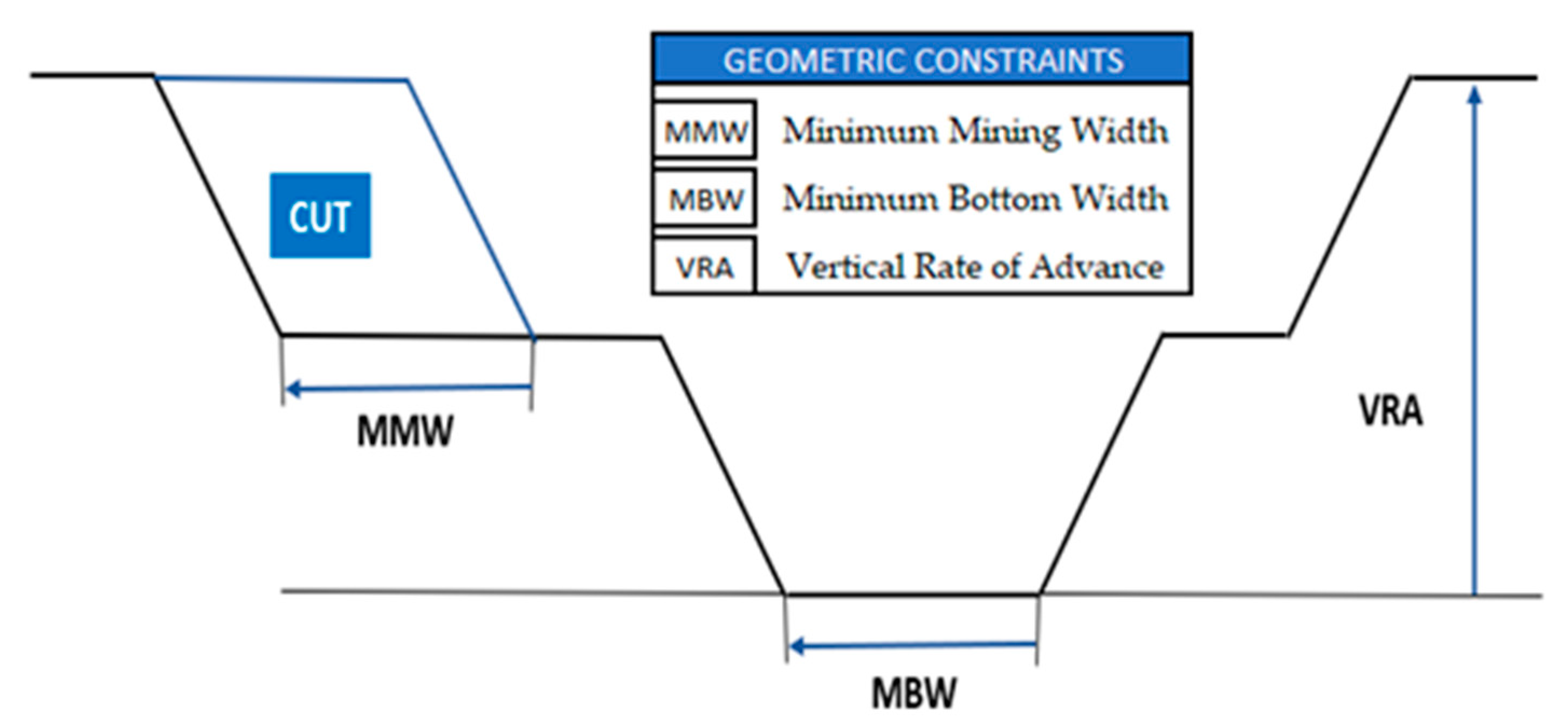
Open pit planning requires the definition of geometric parameters, compatible with the extraction equipment and the required levels of productivity and quality. These constraints ensure the maintenance of the regularity of the pit dimensions. The following geometric constraints stand out [10]: Minimum Mining Width (MMW), Minimum Bottom Width (MBW), and Vertical Rate of Advance (VRA). The MMW refers to the minimum horizontal advance that must be carried out in each period. This restriction must be measured between the slopes of the mine in the direction of expansion of the pit, consecutively for each period. MBW is the horizontal dimension measured at the lowest level (floor) in the open pit in each period. In addition, VRA is the maximum vertical dimension between different mine levels, which can be realized by period. Figure 1 schematically presents these variables.
2.4. Geometallurgy Applied to Mine Planning
Geometallurgy brings together the multidisciplinary efforts of different technological areas. According to Mckee [17], geometallurgical studies allow a broad knowledge of the mineral deposit and its behavior in different processing operations, highlighting the following benefits: economic optimization of operations, modeling of ore behavior in the processing plant, and refinement of mine planning. For Deutsch [18], the objective of geometallurgy is the consistent aggregation of value to the business.
In the technical literature, there are many articles that apply geometallurgical models to mine planning. Studies developed by Gomes, Tomi, and Assis [19] demonstrate that an adequate geometallurgical study is a tool for improving the production plan of a mineral project, redirecting the mining to ore fronts with beneficial performance to the plant. According to Macfalarne and Williams [20], understanding the behavior and distribution of geometallurgical variables in a mineral deposit allows the stabilization and optimization of processing, increasing the operational robustness of the project to respond in scenarios of volatility of prices and demand. Morales et al. [21] performed simulations of the strategic planning of an open pit mine, incorporating the geometallurgical variables grindability and throughput into the block model. Gains up 9.4% were expected in the NPV of the project and reduction in global costs, compared to the results obtained without the assumption of geometallurgical parameters in the model.
Traditionally, the main guiding parameter for mining planning is the grade. In the meantime, the mining engineer seeks to stabilize the feed of the plant, aiming at achieving the products within the specifications required. However, there are other characteristics, intrinsic to each mineral typology, such as specific energy for the comminution of rock fed in the plant. Due to the typological variability of the mineral deposit, variations in the hardness of the rocks may occur and, consequently, significant changes in the productivity and costs of crushing and grinding. Through geometallurgical studies, it becomes possible to model these performance factors and include them in the calculation of the economic value of mining blocks [17]. Another fundamental variable for the performance of the ore during mineral processing is the process recovery. Its geometallurgical characterization is of great importance for mine planning because depending on the lithology processed, the recovery can undergo significant pattern changes. In this way, the proper blending of the ore and the pre-adjustment of the plant to receive these piles are fundamental procedures for maximizing economic gains in mining and processing [22].
According to Kumral [23], certain variables can have important interdependent relationships, such as grade and process recovery, and otherwise, the specific energy of comminution and processing cost. Understanding and modeling these relationships will allow a reduction in geological uncertainties and, consequently, greater assertiveness in carrying out mine planning. Lishchuk et al. [24] carried out studies on the application of geometallurgy in two mines: Mikheevskoye (Russia) and Malmberget (Sweden). The case studies delivered the following findings: correct characterization and testing enable the acquisition of important information about the ore, and the understanding of the mineral particle behavior in mineral processing supports the design of reliable prediction models. According to forecasts, the implementation of a geometallurgical program at the Mikheevskoye mine could reduce the payback by 1.5 years. Geometallurgical studies that map the metallurgical performance of five different iron ore lithologies at the Pau Branco mine can also be highlighted [19]. The knowledge obtained allowed the elaboration of a new mine production plan, which generated a positive increment equal to USD 25.6 millions in the NPV. Reis et al. [25] developed a study to estimate and minimize the risks involved in the Mineral Resource and Mineral Reserves (MRMR) stages, considering the variability of the bulk density in mining planning. Such a study was applied in an iron ore mine, showing gains of 5% in LOM and 2% in NPV.
Wambeke et al. [26] presented a new estimating approach for the Bond Ball Mill Work Index as a geometallurgical variable, applied to the Tropicana gold mine. It was possible to obtain gains of up to 72% in the mine production forecasts. Nunes et al. [27] proposed a new methodology capable of consolidating different approaches regarding the geometallurgical information of a mineral deposit. This model was applied in a copper and gold mine located in Brazil. Evaluating different blasting and processing scenarios through the pit-to-plant approach, it was possible to increase the throughput of the plant by 10.7%, in addition to a gain of 2.2% in the crusher feed rate.
Rodrigues et al. [28] carried out studies correlating the geological model of an iron ore deposit with tests to determine energy consumption in grinding for each mineralized lithology. Based on these studies, a mathematical model was defined to calculate the specific comminution energy, inserting this variable in the block model of the deposit.
The company Hot Chilli, the owner of the copper, gold, and molybdenum mines of the Productora project, located in the northeast region of Chile, has developed a geometallurgical model to predict the processing responses of sulfide and oxidized ores. This geometallurgical model incorporates results from mineralogical, metallurgical, and comminution tests developed for samples collected from different geological domains of the deposit. Through this model, the hourly production rates and costs of the comminution circuit were estimated [29].
3. Materials and Methods
3.1. Block Model
In this section, the parameters related to the block model are presented. In a special way, the distribution of the geometallurgical variables is detailed.
3.1.1. General Information
The block model used is owned by the company BNA Mining Solutions and is composed of 102,789 blocks with dimensions equal to 10 m × 10 m × 10 m. The model represents an iron ore deposit in the Iron Quadrangle, located in the Brazilian state of Minas Gerais. It has, as geometallurgical variables, process recovery (%) and specific energy (kWh/t) values for each block.
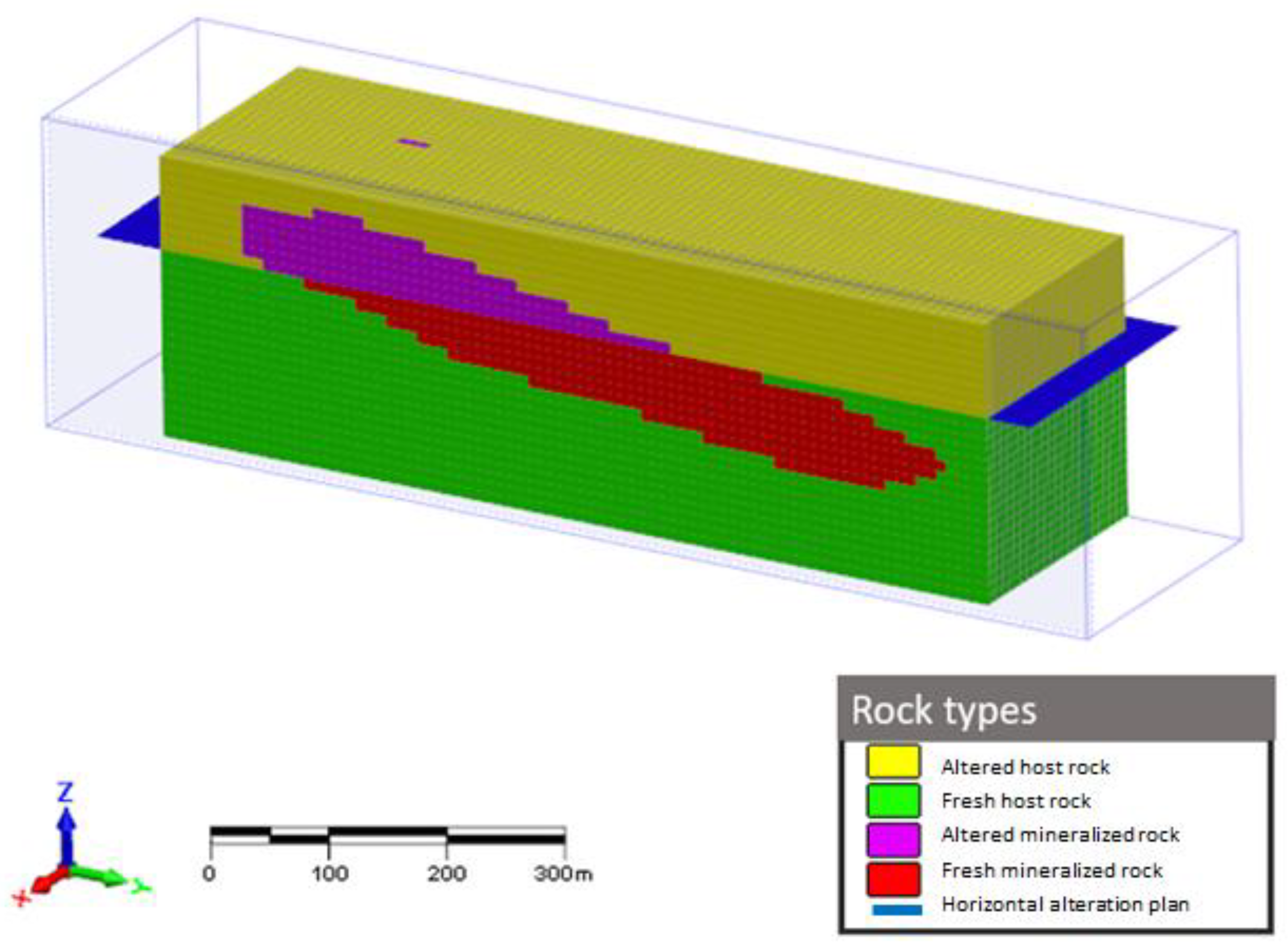
As part of the construction of the block model, a horizontal alteration plan (represented in blue) was considered, dividing the volume of the model into 4 different lithologies: altered host rock; fresh host rock; altered mineralized rock; and fresh mineralized rock. The term “mineralized rock” refers to lithologies that have different iron grades, and “host rock” refers to lithologies that do not contain any iron. Figure 2 shows a three-dimensional view of the block model under study, identifying the alteration zone and the different lithologies present.
The slope angle and density variables have different values for each of the lithologies, relative to their respective geomechanical behavior. Table 1 shows the densities and slope angles for the lithologies in the model.
3.1.2. Geometallurgical Parameters
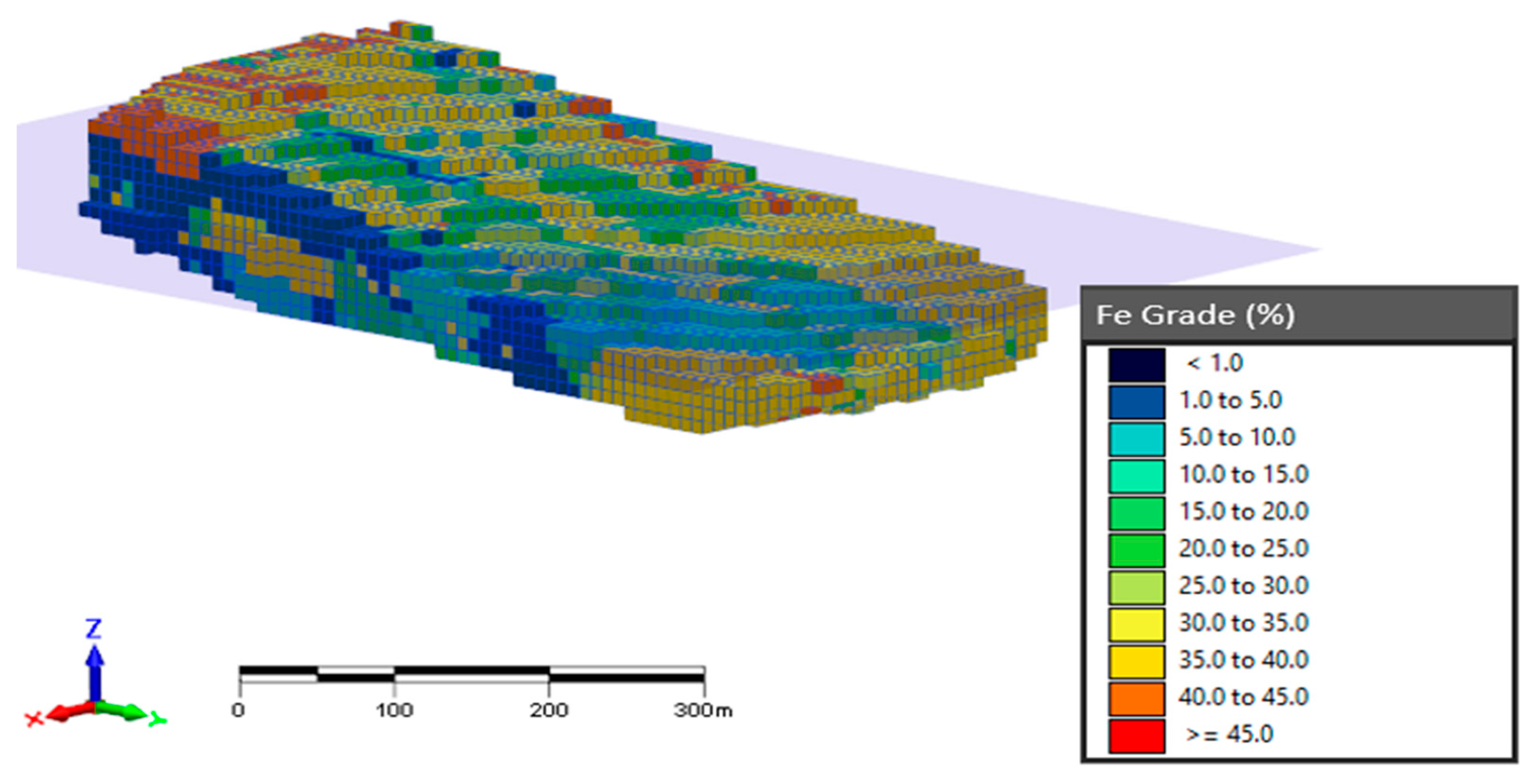
Through Figure 3, it is possible to visualize the distribution of Fe grades along the mineralized body.
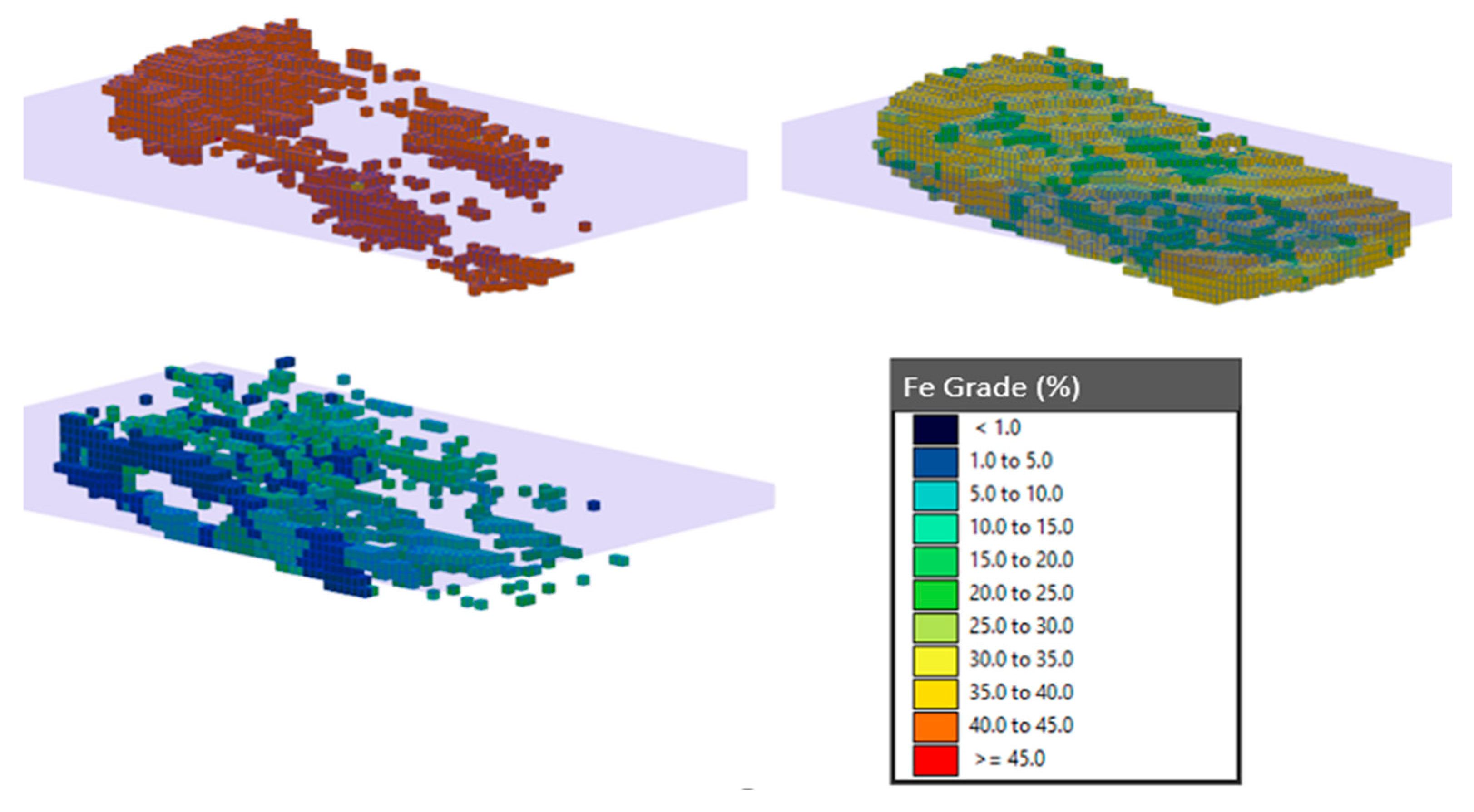
The existence of regions with a preponderance of grades within certain ranges can be seen. Figure 4 shows the blocks with Fe grades above 40% (top left), between 20% and 40% Fe (top right), and below 20% Fe (bottom left).
Therefore, the richest blocks (above 40% Fe) predominantly occur in the upper outer part of the block model (altered mineralized rock) and in the lower outer part of the block model (fresh mineralized rock). The blocks with intermediate grades (between 20% and 40% Fe) occur in the inner part (core) of the block model, going from the altered mineralized rock to the fresh mineralized rock in a relatively homogeneous way. In turn, the poorest blocks (below 20% Fe) are dispersed in the outer part of the block model, from the altered mineralized rock to the fresh mineralized rock, occupying the spaces between the richer blocks and covering the blocks of intermediate grades.
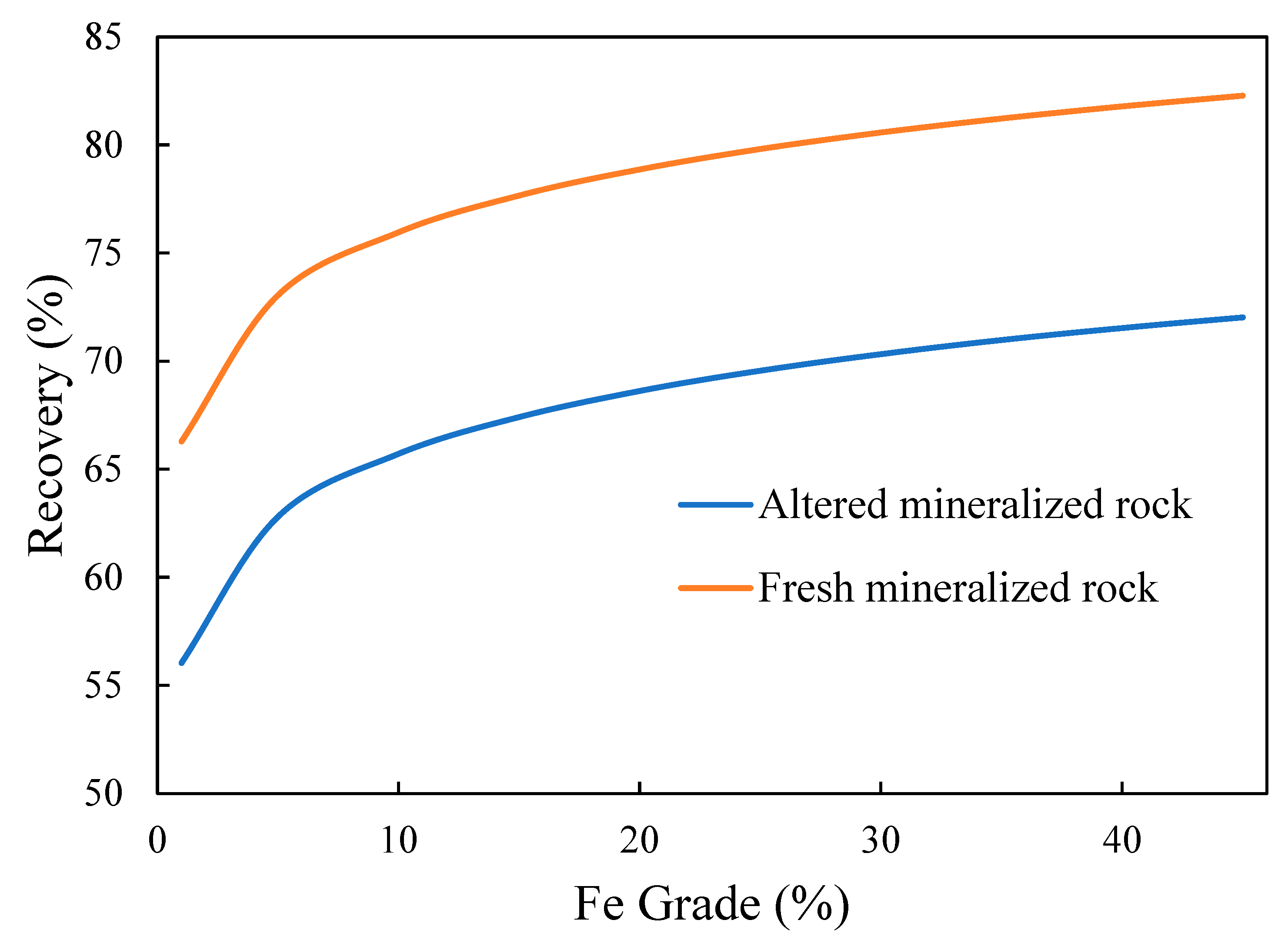
Carrasco, Chilès, and Séguret [30] demonstrated that the recovery parameter is non-additive, and its spatial variability by geostatistical methods cannot be modeled with any reliability. On the other hand, studies conducted by Wheaton [31] demonstrated correlations between the process recovery variable and ore grade. For the present iron ore deposit, the strategy used was to carry out concentration tests for ores of different grades, generating logarithm regression curves. Equations (3) and (4) correlate the grade of each block with the process recovery variable, respectively, for the altered mineralized rock and fresh mineralized rock lithologies.
where RFe = process recovery (%); tFe = Fe grade (%).
Figure 5 presents the grade and recovery correlation curves for the block model.
It can be seen that, for the same grade range, the altered mineralized rock presents smaller recoveries on the plant than the fresh mineralized rock. Figure 6 shows the distribution of process recoveries in the block model.
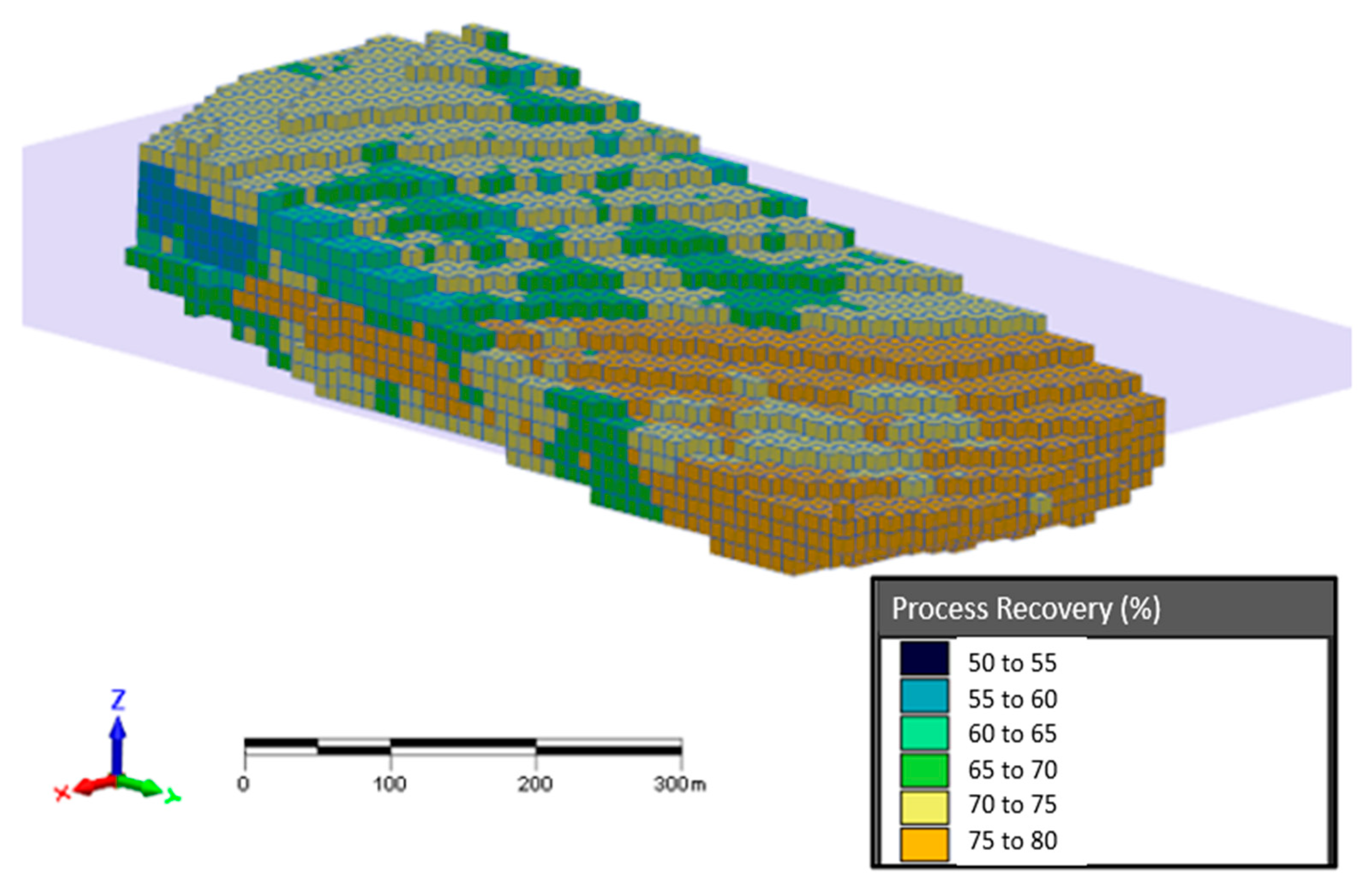
It is possible to see the existence of regions whose blocks present distinct ranges of recovery. Figure 7 shows the blocks belonging to the following ranges: above 75% (upper left), between 65% and 75% (upper right), and below 65% (lower left).
As shown in Figure 7, most blocks of the fresh mineralized body (lithology located below the alteration plane) show recoveries above 75%. Blocks with intermediate recoveries (between 65% and 75%) occur predominantly in the altered mineralized rock and in the outer walls of the fresh mineralized rock. The low recovery blocks (below 65%) occur in the transition region between the altered and fresh mineralized rocks, embedded in the intermediate recovery blocks.
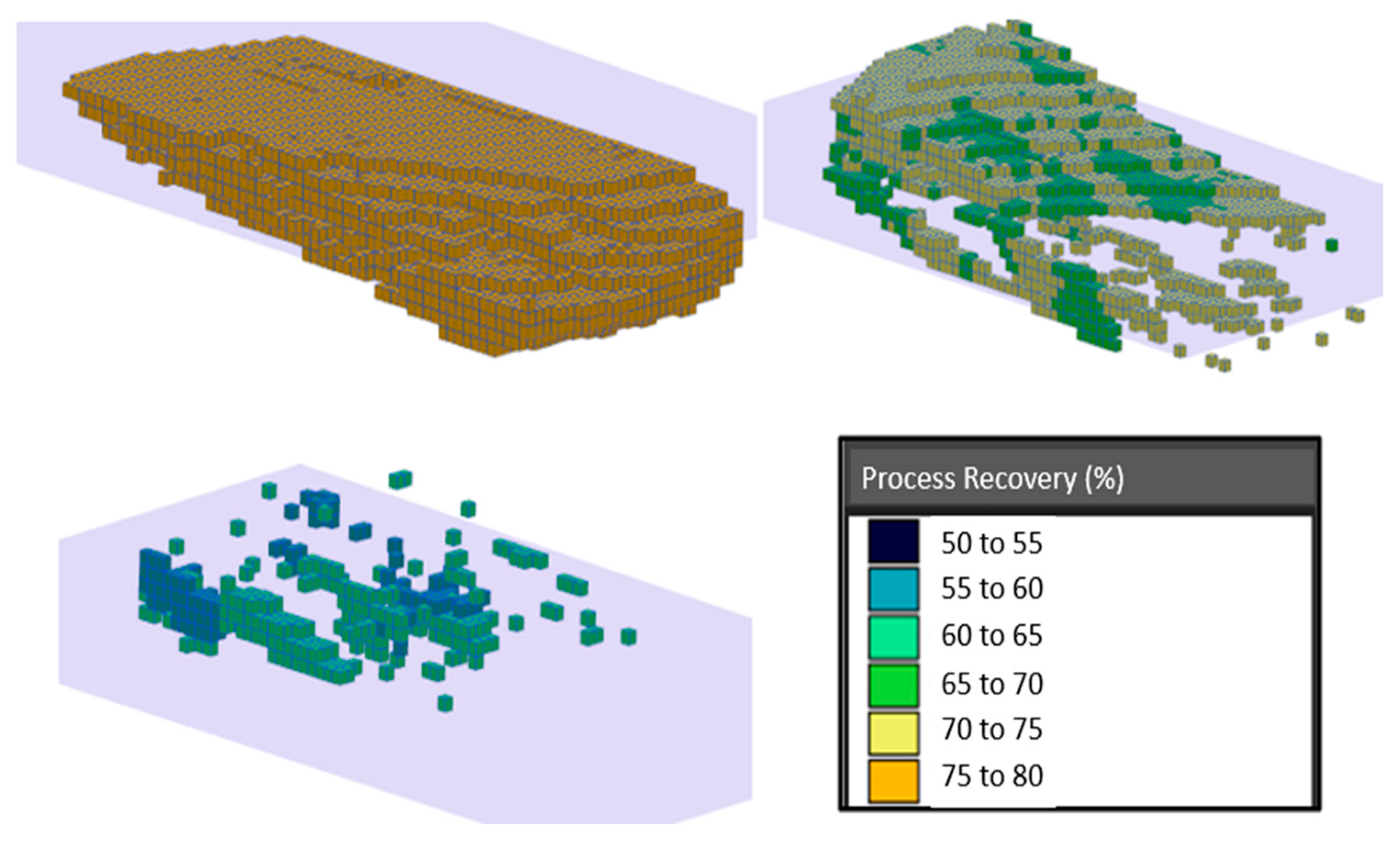
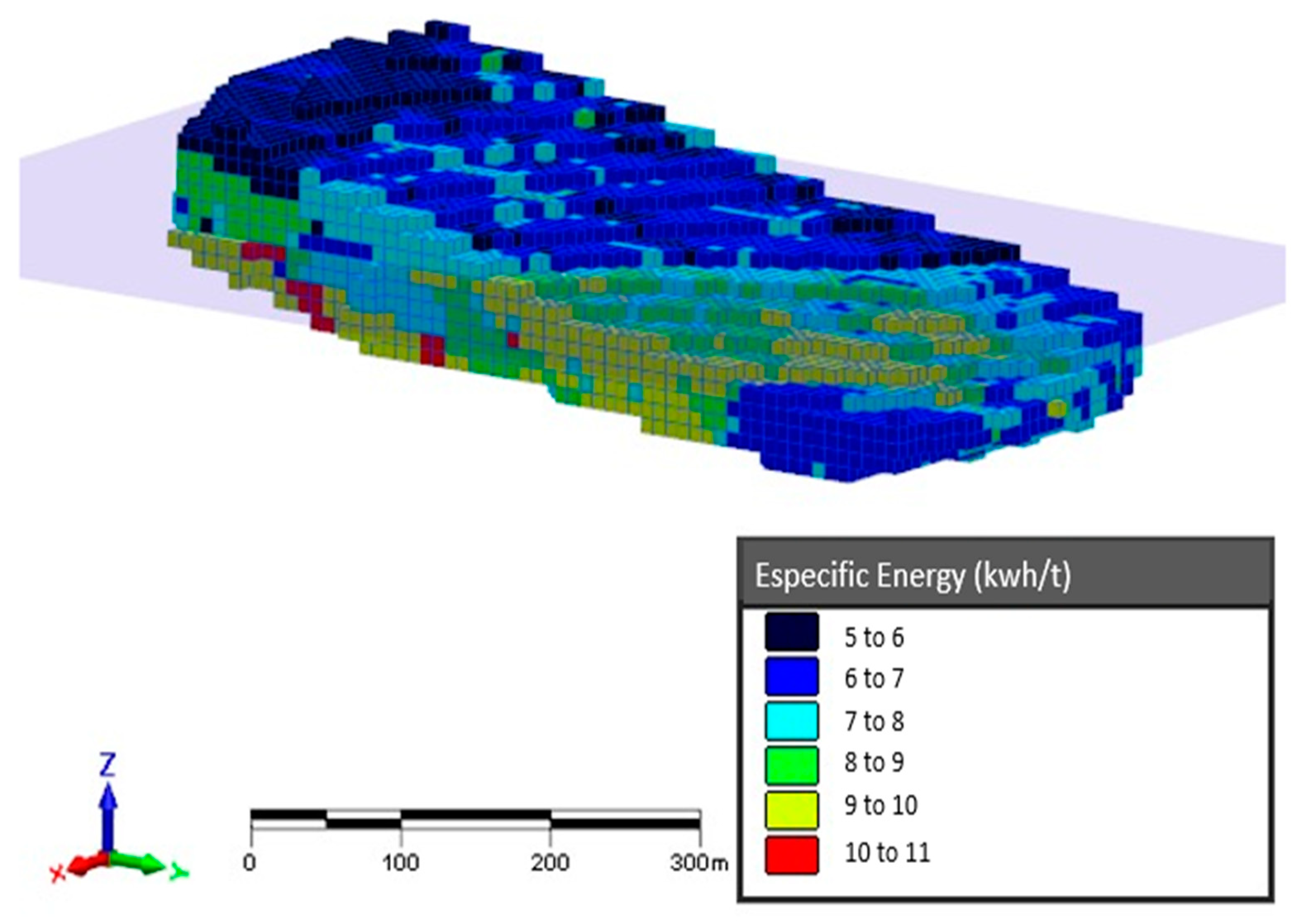
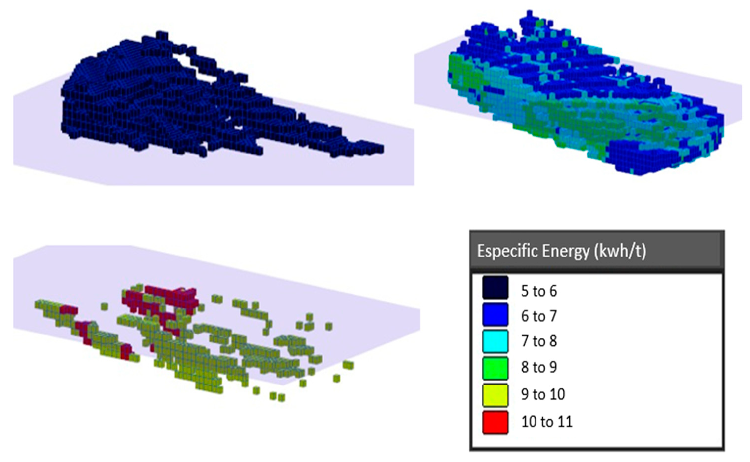
Studies developed by Rodrigues [32] in an iron ore deposit in Minas Gerais state, Brazil, showed that the variable specific energy of comminution obtained in a custom laboratory grinding test, designed specifically for this deposit, can be considered as additive, allowing the use of linear interpolation methods. Figure 8 presents the distribution of specific energies for the block model.
Figure 9 allows the visualization of three distinct energy bands: below 6 kWh/t (top left), between 6 kWh/t and 9 kWh/t (top right), and above 9 kWh/t (bottom left).
It appears that the lowest specific energies (below 6.0 kWh/t) are located only in blocks of the altered mineralized rock (lithology above the alteration plane). Intermediate energies (between 6.0 and 9.0 kWh/t), in turn, encompass most blocks of the model and are distributed along the two mineralized lithologies. Otherwise, the highest specific energies (above 9.0 kWh/t) are located in sparse regions in the fresh mineralized rock.
3.2. Scenarios
This study aimed to analyze the insertion of geometallurgical variables to build more realistic and feasible mine planning. Three different scenarios were built: Base Case scenario (BC), where the recovery was fixed and the specific energy was not taken into account; GeoMet1, where the recovery varied according to the BNA model and the specific energy was disregarded; and GeoMet2, in which the process recovery and specific energy were taken into account according to the original distribution in the block model.
3.2.1. Base Case (BC) and GeoMet1 Scenarios
Table 2 shows the operational constraints and economic parameters applied to the BC and GeoMet1 scenarios.
Therefore, the only assumption that differs between BC and GeoMet1 is that the first scenario contemplates fixed recoveries at 78% for all blocks, while GeoMet1 distributes the variable recovery according to the BNA block model. In order to verify the efficiency in achieving ore masses produced over the lifetime of the project, a % of compliance above 90% was defined as a target.
3.2.2. GeoMet2 Scenario
For the GeoMet2 scenario, the parameters from Table 2 related to GeoMet1 were considered; however, the specific energy variable was contemplated in the block model. In this way, the process cost varies according to the specific energy in comminution (kWh/t) of each block.
For the iron ore processing plant, the power (P) capacity installed in the comminution circuits is 2100 kW. Each block has its specific energy (SE), so the respective Throughput (T), in t/h, is calculated by Equation (5).
The individual processing time (TP), in hours, is calculated by Equation (6).
The mass M, in tons, is equal to where d is the density in situ of each block (t/m3).
Considering specific energies and different densities in situ for each block, there are different values for the values of M and T, which impacts the distribution of the TP variable along the mineralized lithologies. To measure and limit the maximum annual processing time of the plant (hours), the following annual operating regime was adopted: 365 days per year, 24 h a day, and an operating yield of 90%. Thus, the global processing time (TGP) is equal to h per year.
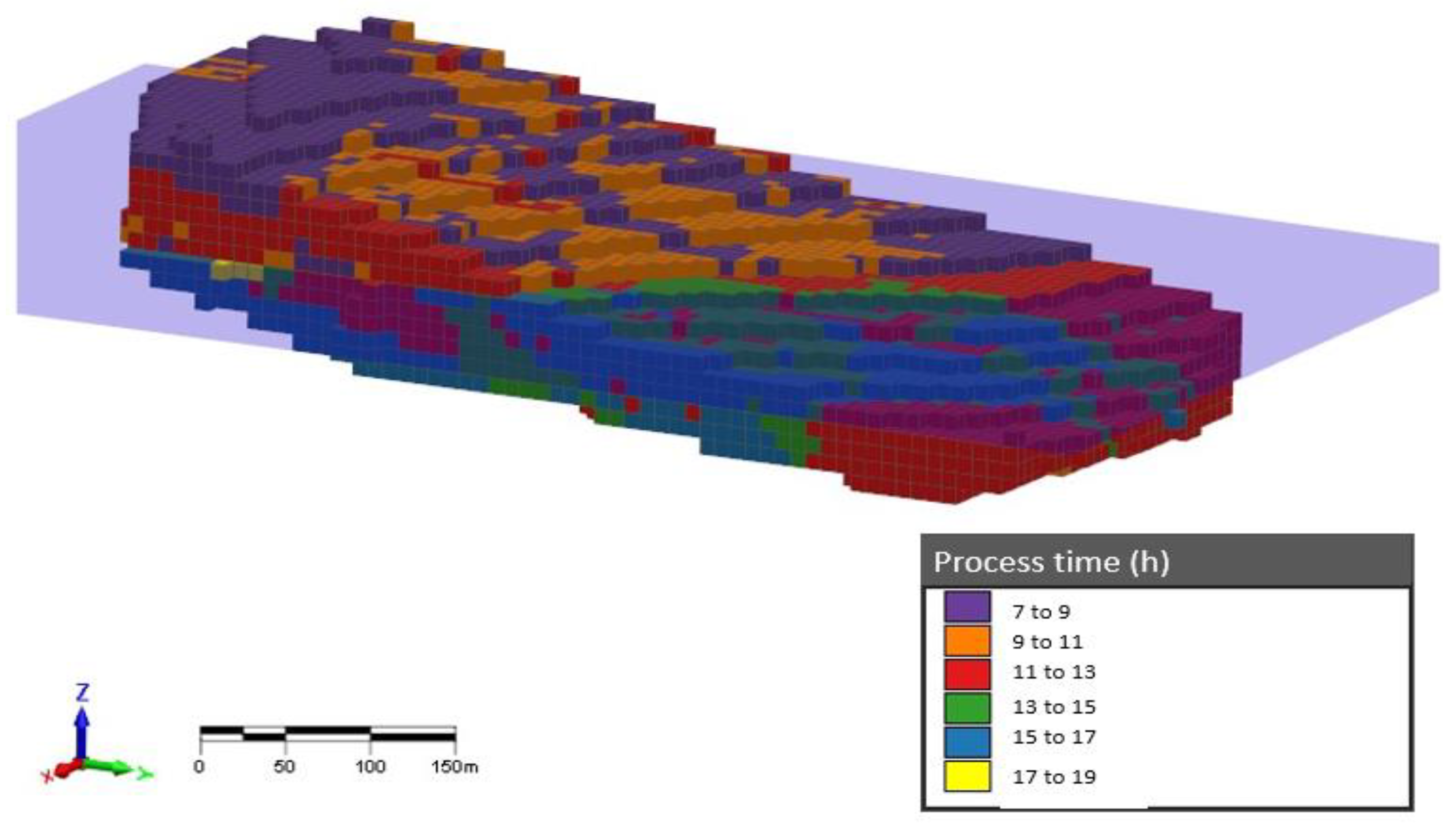
Figure 10 allows for the visualization, in a global way, of the different ranges of processing times (TP) present in the blocks of the model.
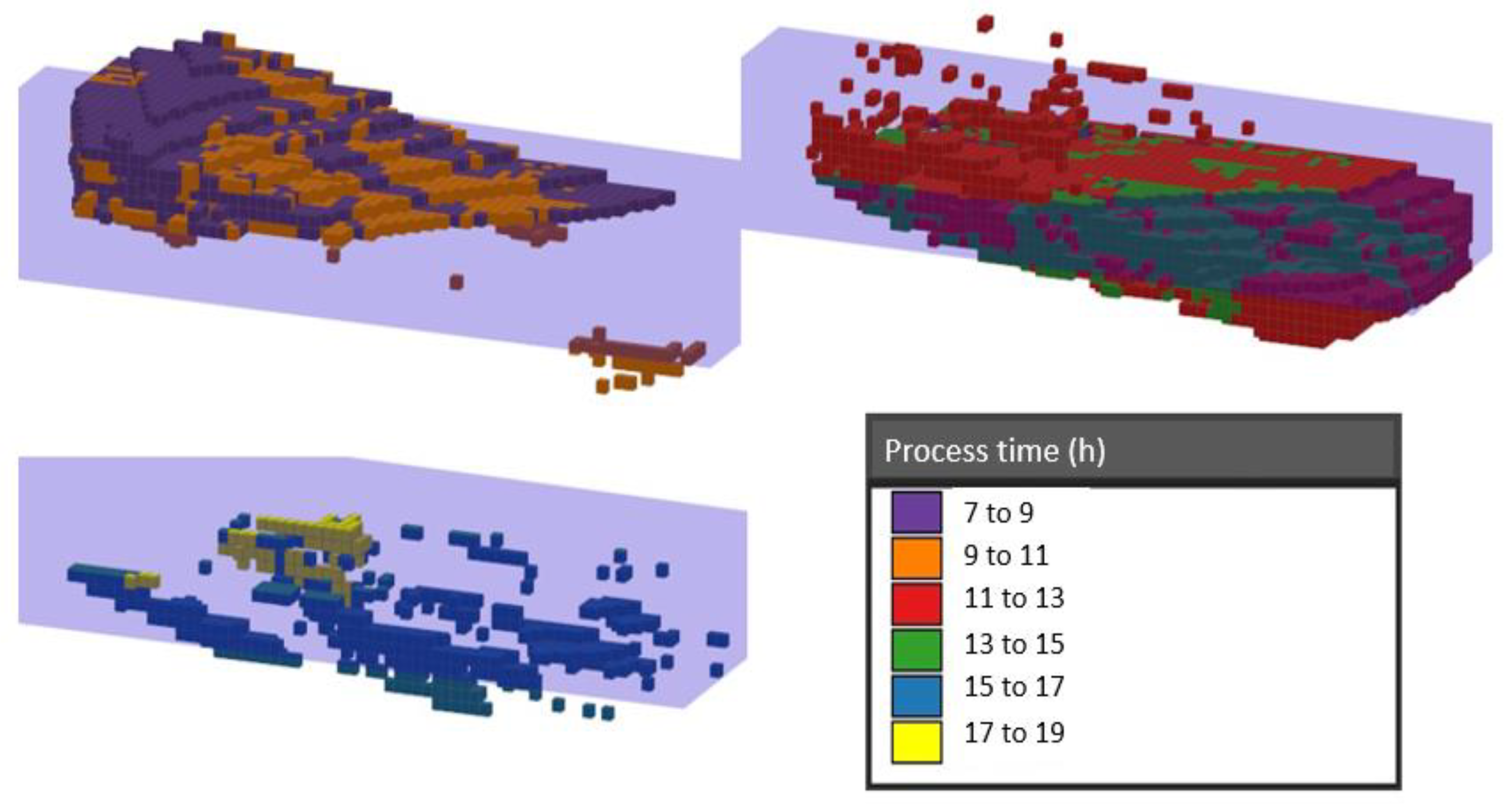
Figure 11 focuses on three distinct PT intervals: below 11 h (upper left side), between 11 and 15 h (upper right side), and above 15 h (lower left side).
There is a preponderance of blocks with smaller TP in the altered mineralized body, with some blocks in this category located in the fresh mineralized rock. Regarding the intermediate TP blocks, these are located mainly along the fresh mineralized rock, with a smaller number of sparse blocks in the altered mineralized body. Higher TP blocks, in turn, occur in small groups, embedded with intermediate TP blocks along the fresh mineralized rock.
It is noteworthy that the variation in processing time causes changes in the respective process cost. This relationship can be justified by the fact that a block with longer residence time in the plant will bring increased wear to equipment (notably crushers and mills, present in the comminution circuit), as well as lead to increased consumption of electricity and other inputs directly applied to mineral processing, such as grinding bodies. Therefore, this study took into account the variability of the process cost parameter as the TP changes per block.
The global average processing time for the block model mineralized lithologies is 11.07 h. This TP was attributed a processing cost of 15 USD/t. From this relationship, the process cost for each block was calculated directly proportional to the TP of each block. Table 3 presents the average values of the process cost and processing time per block, for each mineralized body.
3.3. Software for Integrated Optimization
The MiningMath software version v2.2.14 is based on the Integrated Optimization approach and it was used to build the scenarios for this work. In this software, each block of the model was referenced by its geographic coordinates (X, Y, and Z), Fe grades (%), economic values (USD), density (t/m3), slope angle (degrees), process recoveries (from 0 to 1), and processing time (hours). The destination (plant, stockpile, or waste dump) of each block is defined by the software, depending on the economic values and grades contained in the blocks [10].
For information, the Doppler software is also based on Integrated Optimization. This was developed by the DELPHOS Laboratory at the University of Chile. Its differential in relation to MiningMath is the possibility of performing mine planning using both the LG and DBS approaches. Doppler considers several constraint modalities, such as slope angles, capacity for each system parameter, blending, multi-destinations, and ore stockpiles [33]. However, the authors did not use it because it was not available at the time.
3.4. Block Economic Value
Equations (7) and (8) present the block economic value for, respectively, ore and waste blocks.
where: Process = economic value of ore blocks (USD); MB = block mass (t); tFe = Fe grade (%); RFe = process recovery; PVFe = Fe selling price (USD/t); CP = process cost (USD/t); and CM = mine cost (USD/t).
where: Waste = economic value of waste blocks (USD).
4. Results and Discussion
4.1. Global Results
Table 4 displays the overall results of the simulations. It is noteworthy that different lifetimes were found for BC and GeoMet scenarios. Therefore, to equalize the analysis of the financial return, the Annualized Net Present Value (ANPV) was determined. This result transforms the cash flow of the project into a uniform series, presenting the monetary gain obtained by period (years in this case) and thus allowing an adequate comparison between different LOMs. Mariz et al. [34] demonstrated that the ANPV is a reliable parameter for the economic evaluation and selection of the best alternative among mine excavation and transport equipment. The ANPV can be calculated using Equation (9).
where i = discount rate (%); and n = number of periods.
4.2. Graphical Analysis
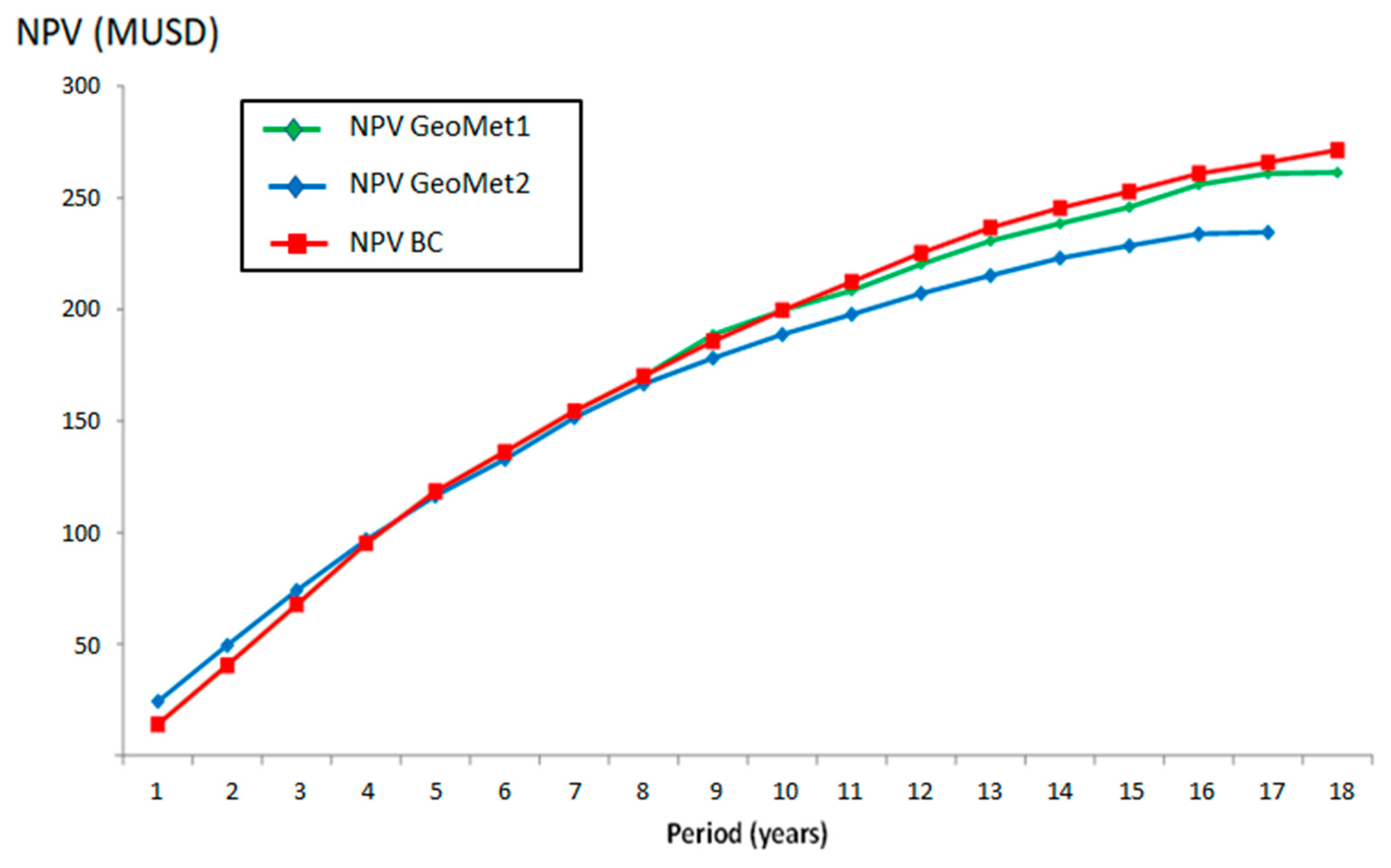
In Table 4, BC scenario gains are shown in relation to the GeoMet1 and GeoMet2 scenarios, for both NPV and ANPV. Therefore, the comparative analysis of the evolution of the NPV along the LOM is valid. Figure 12 presents the comparison of the NPV curves.
The GeoMet1 and GeoMet2 scenarios delivered a final NPV, respectively, 3.68% and 13.57% lower than the BC scenario. Until year 8, the GeoMet1 and GeoMet2 NPV curves showed comparable values in relation to BC, but from year 9 the BC started to show increasing relative gains. Such behavior is due to the fact that BC does not consider the geometallurgical variable specific energy in the simulation, in addition to setting the same recovery (78%) for all blocks. In this form, there is no recovery oscillation depending on the region where the ore extraction takes place, and the process cost parameter remains constant and equal to 15 MUSD/t during the simulation as well. Thus, the BC scenario does not include financial losses to the project due to the geometallurgical distribution of the variables in each block. For GeoMet2, the comparative reduction in NPV in relation to BC is 3.69 times greater than for GeoMet1. In this way, the variable specific energy significantly increases the complexity of the mine planning to be developed. The assumptions adopted by GeoMet2 are more reliable and closer to reality, so the lower NPV result is feasible and allows greater assertiveness in strategic mine planning.
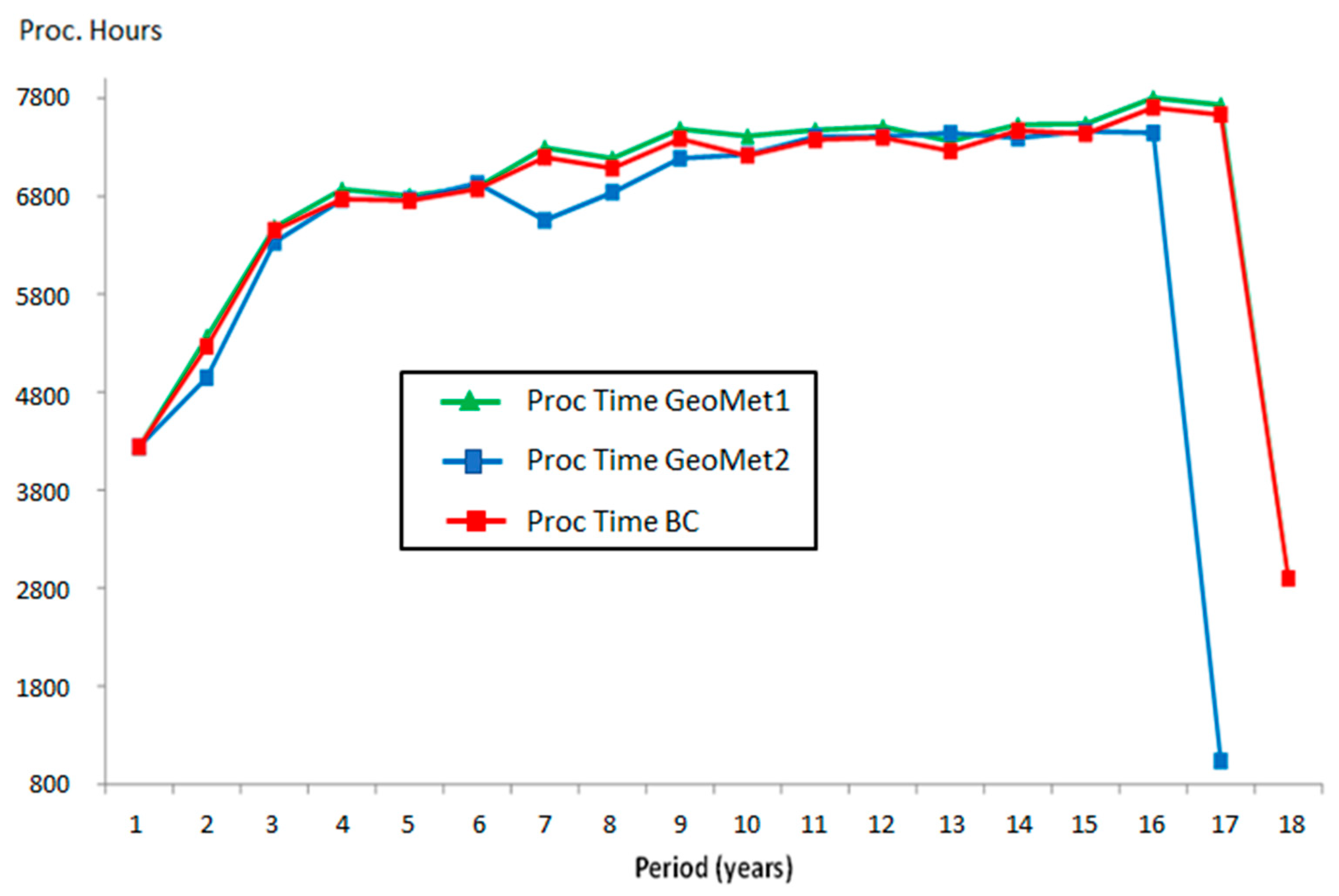
Figure 13 presents the evolution of global processing hours, for scenarios simulated. For the BC and GeoMet1 scenarios, the processing time values were accumulated and provided by the simulation report, although the specific energy was not considered to guide mine scheduling.
Figure 13 demonstrates that, for three scenarios, there is a gradual increase in the annual processing time of the plant during the life of the mine (LOM). When analyzing Figure 11 (Detailing of processing time intervals), it is noted that the processing times per block tend to increase in the lower levels of the deposit, consistent with the deepening of the open pit over time. The global average of this parameter, for GeoMet1, showed a positive difference of only 1.25% in relation to BC. For GeoMet2, this deviation was 8.06% less. The reason is the fact that GeoMet2 was oriented towards reducing the consumption of processing hours, considering a proportional dependence between this variable and the process cost. For the BC and GeoMet1 scenarios, this strategy is not taken into account, as they did not include the specific energy in the block model.
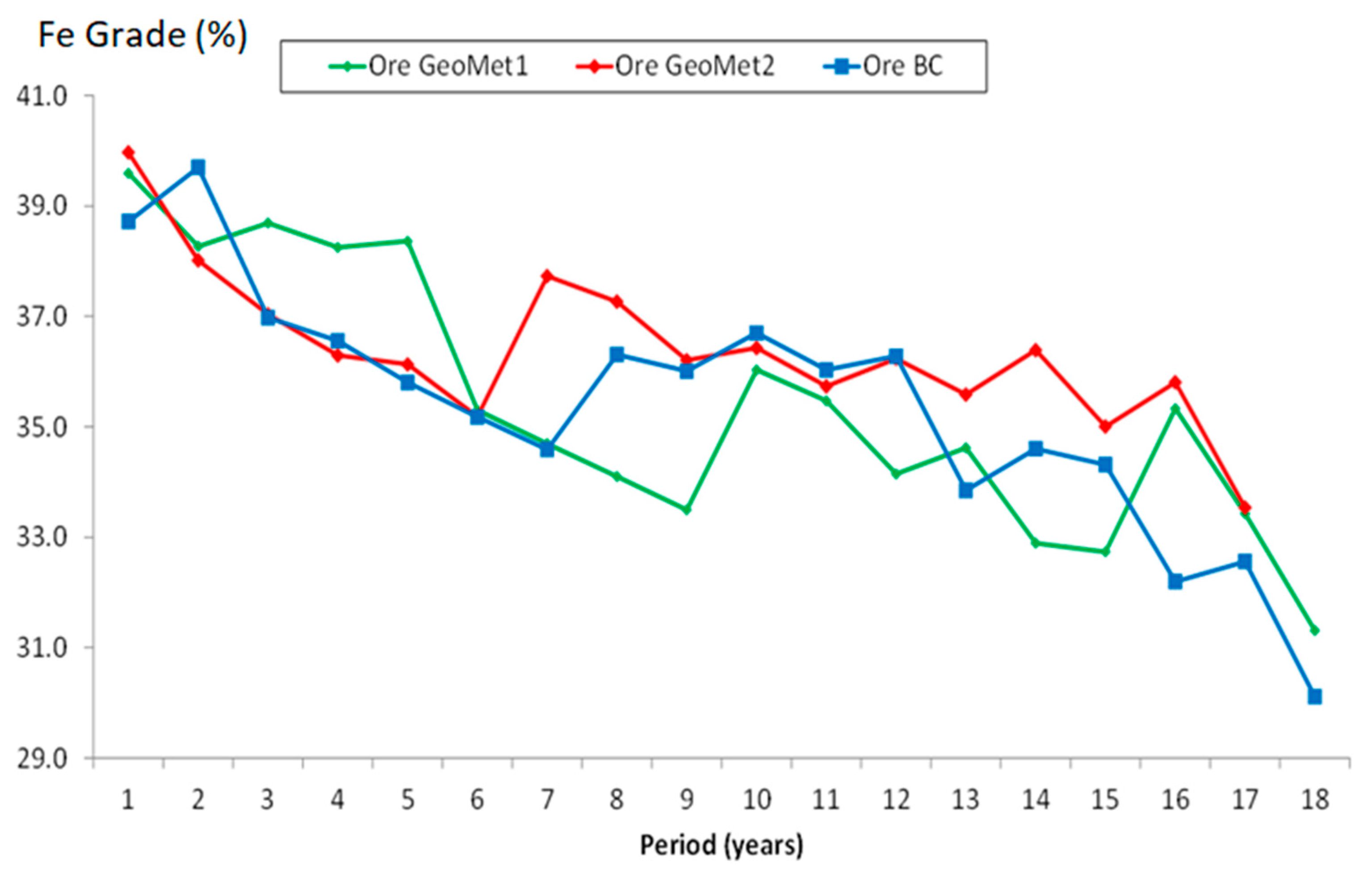
Figure 14 displays the annual averages of Fe grades for BC, GeoMet1, and GeoMet2 scenarios.
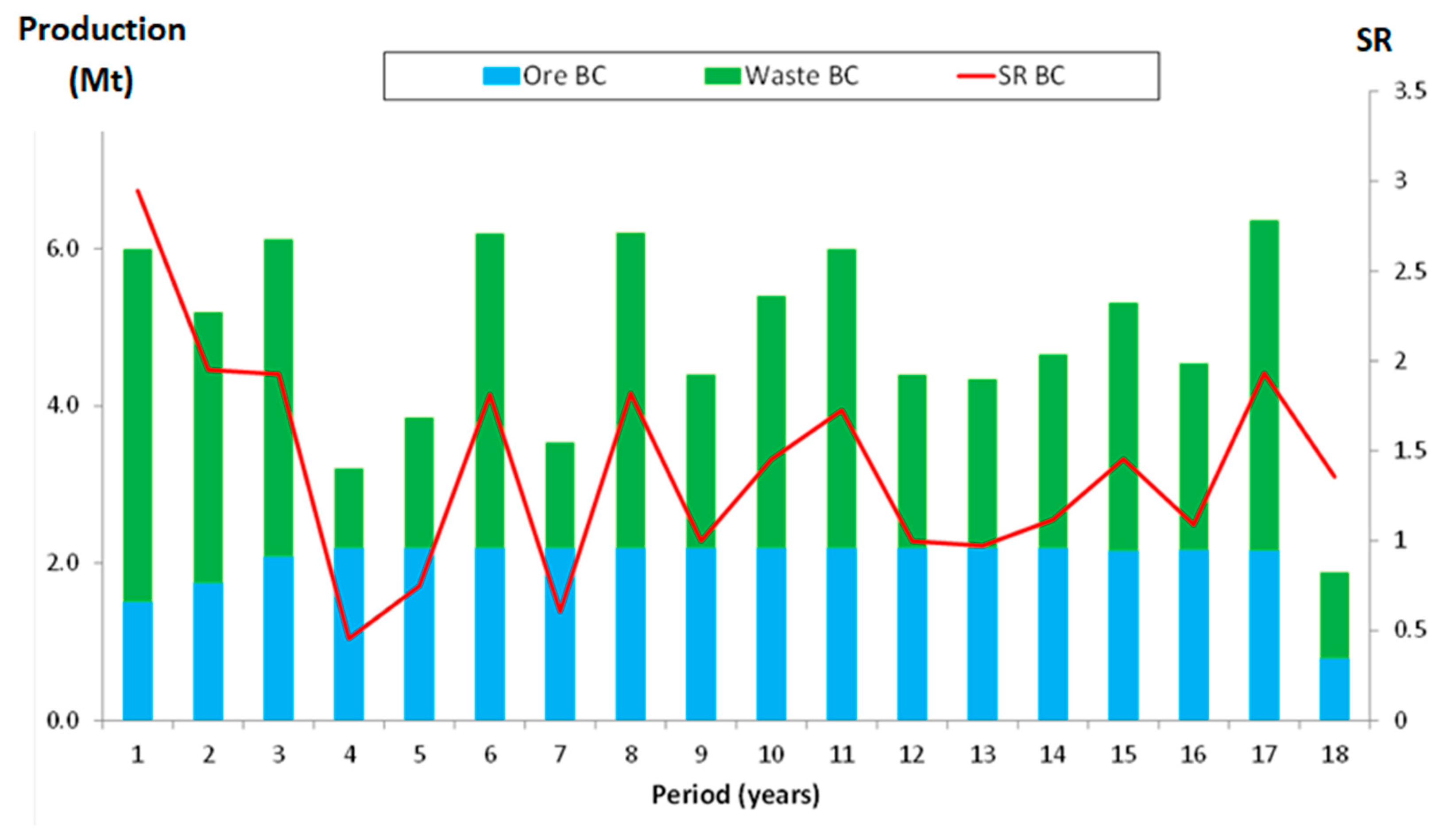
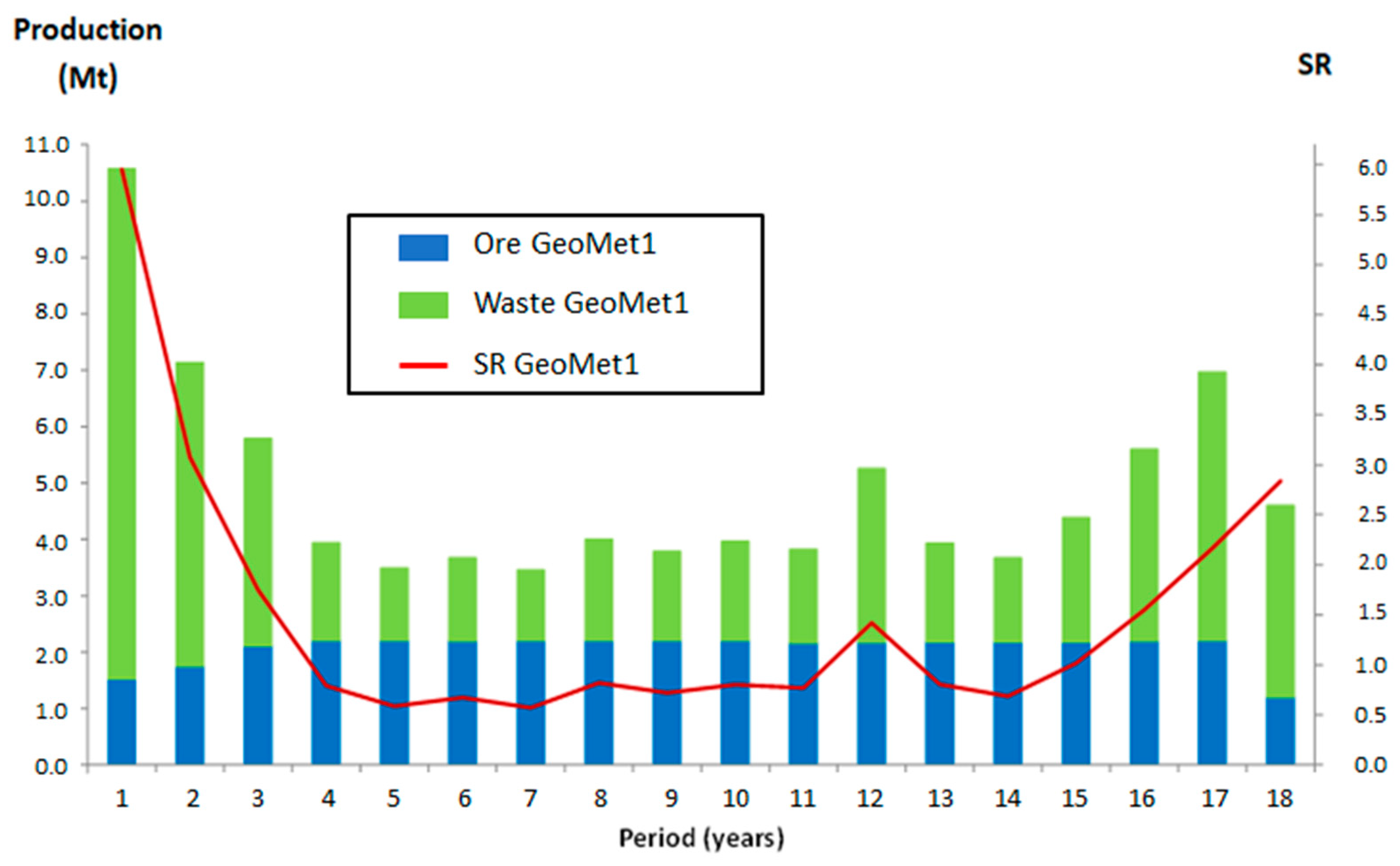
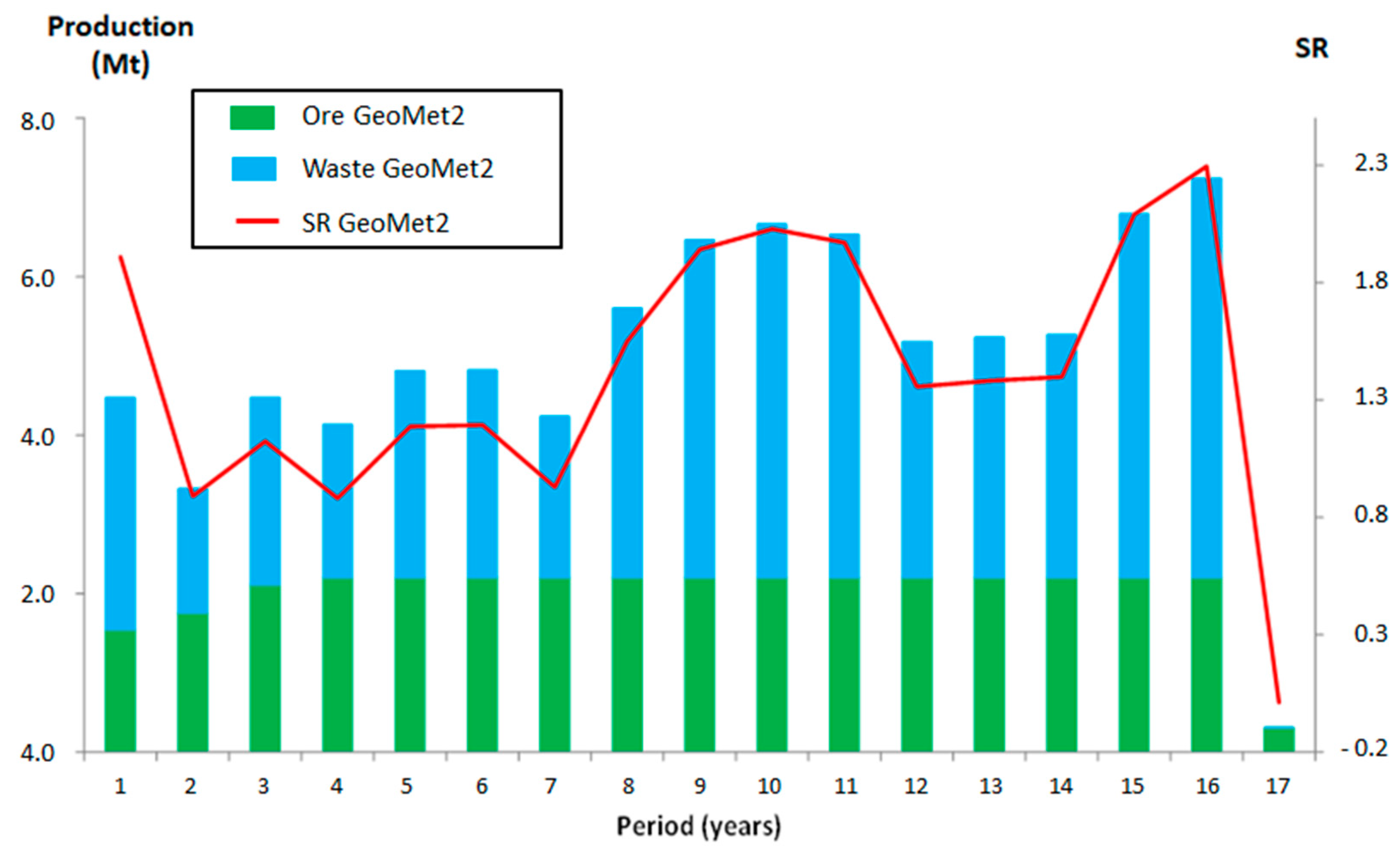
It appears that both scenarios managed to reach annual averages of grades in the specification of plant feeding (30% and 40%), with a tendency to prioritize richer and more profitable blocks in the first years of the LOM. This characteristic is accentuated for GeoMet1 and GeoMet2 scenarios, as they consider variable recoveries according to the BNA block model. In this way, the algorithm searches for blocks with higher recoveries, favoring better revenues for the project. It should be noted that the GeoMet2 scenario had an overall average 2.88% higher than the BC. This result demonstrates an efficient strategy for extracting richer blocks, aiming to achieve higher revenues, and thus offsetting the increase in block-by-block process costs. On the other hand, an abrupt drop in the Fe grade can be noticed from year 6 onwards in the BC scenario. Figure 15, Figure 16 and Figure 17 show the evolution of ore and waste production, in addition to the Stripping Ratio (SR).
Both scenarios achieved the predicted % compliance, reaching above 90% of the expected ore masses during and after the ramp-up. Regarding the Stripping Ratio (SR), the BC presented about 3.0 in the first year, decreasing afterward and oscillating in values between 0.5 and 2.0 until year 8 and then oscillating between 1.0 and 2.0 at the end of the project. In the case of GeoMet1, the SR started at around 6.0, dropping to values close to 0.5 until year 7 and rising to levels between 1.0 to 3.0 by the end of the project. For GeoMet2, the SR started at around 1.8, dropping to levels around 1.0 by year 7 and then rising to values as high as 2.3 by year 16.
Thus, it is noted that GeoMet2 required more mine development than BC, reflecting the need to open more mining fronts due to the variability of recovery parameters and processing time throughout the deposit. The global SR, for GeoMet2, was 9.20% higher than BC, contributing to a lower NPV achieved. Therefore, the GeoMet2 scenario is more realistic and allows for anticipation of the operational challenges of the project.
5. Conclusions
The present work allowed us to demonstrate the importance and relevance of working with block models built with geometallurgical variables. The use of assumptions that do not reflect the complexity of the mineral deposit can cause serious errors in strategic mining planning. As the main results, GeoMet2 and GeoMet1 scenarios presented NPVs, respectively, 3.68% and 13.57% lower than the BC scenario. In terms of ore production, the respective differences found for GeoMet1 and GeoMet2 were +1.03% and −6.97% in relation to BC. In other words, the BC results could overestimate the financial and production results, denoting the importance of using geometallurgical variables for generating reliable and realistic ultimate mine designs and scheduling. Such NPV and ore production numbers from BC are notably overestimated in relation to GeoMet2, which contemplates additionally the specific energy distributed according to the BNA model.
It is important to point out that the arbitrated recovery value for the BC scenario influences the financial gain or loss in relation to GeoMet2. If a greater recovery were adopted (optimistic scenario), the apparent financial gain would be higher. In the case of adopting a much smaller recovery than the effective potential of the deposit (pessimistic scenario), such a difference would decrease or even be negative in relation to GeoMet2. In all these options, it can be seen that GeoMet2 is more reliable than BC, as it considers the heterogeneous distribution of the variables recovery and specific energy, inherent to existing lithologies.
In the BC scenario, the process recovery was constant for all blocks, and the specific energy of comminution was disregarded. For the GeoMet1 scenario, the variable recovery was distributed according to the block model used. In turn, for GeoMet2, both the variables recovery and specific energy were considered and inserted in each block according to criteria defined in the construction of the model. It was also found that the GeoMet2 impacted the average annual processing time of the plant by 6.91% less than the BC since the simulation was directed to reduce the process costs caused by the specific energy variable. Otherwise, the stripping ratio of the GeoMet2 scenario was 9.20% higher, due to the need for further mine development to enhance the mine scheduling.
It was possible to identify that the geometallurgical scenarios are more realistic and reliable than scenarios that do not consider the real complexity existing in mineral deposits. This is relevant for industry and academia, encouraging the construction of more detailed block models and considering geometallurgical variables such as process recovery and specific energy. In addition, the Integrated Optimization methodology showed good operability in both scenarios, demonstrating the possible use in future mine planning scenarios. The paper presents answers to important questions about the challenges faced in mining, demonstrating that assertive geometallurgical modeling is essential to guide assertive mine planning.
Author Contributions
Conceptualization, J.F.C.d.M. and D.B.M.; Methodology, J.F.C.d.M. and D.B.M.; Software, A.S.N.; Validation, A.S.N. and D.B.M.; Formal analysis, D.B.M.; Investigation, J.F.C.d.M.; Resources, A.S.N.; Data curation, A.S.N. and D.B.M.; Writing—original draft preparation, J.F.C.d.M.; Writing—review and editing, A.S.N. and D.B.M.; Visualization, J.F.C.d.M.; Supervision, D.B.M.; Project administration, D.B.M.; Funding acquisition, J.F.C.d.M. All authors have read and agreed to the published version of the manuscript.
Funding
This research was funded by CNPq–National Council for Scientific and Technological Development, grant number 142445/2018-5.
Data Availability Statement
Not applicable.
Acknowledgments
The authors would like to thank MiningMath for providing a software license for the simulations and BNA Mining Solutions for the cession of the block model.
Conflicts of Interest
The authors declare no conflict of interest.
References
- Hustrulid, W.; Kuchta, M. Open Pit Mine—Planning & Design, 2nd ed.; Balkema: Rotterdam, The Netherlands, 2006. [Google Scholar]
- Whittle, D.; Whittle, J.; Wharton, C.; Hall, G. Strategic Mine Planning, 8th ed.; Gemcom Software International Inc.: Vancouver, BC, Canada, 2005. [Google Scholar]
- Poniewierski, J. Block Model Knowledge for Mining Engineers—An Introduction; Deswik Technical Report; Deswik: Brisbane, Australia, 2019. [Google Scholar]
- Lishchuk, V. Geometallurgical Programs—Critical Evaluation of Applied Methods and Techniques. Licentiate Thesis, Department of Civil, Environmental and Natural Resources Engineering, Luleå University of Technology, Luleå, Sweden, 2016. [Google Scholar]
- Dominy, S.C.; O’Connor, L.; Parbhakar-Fox, A.; Glass, H.J.; Purevgerel, S. Geometallurgy—A Route to More Resilient Mine Operations. Minerals 2018, 8, 560. [Google Scholar] [CrossRef] [Green Version]
- Elkington, T.; Durham, R. Integrated open pit pushback selection and production capacity optimization. J. Min. Sci. 2011, 47, 177–190. [Google Scholar] [CrossRef]
- Lerchs, H.; Grossmann, I.F. Optimum design of open pit mines. In Proceedings of the Joint CORS and ORSA Conference, Montreal, QC, Canada, 27–29 May 1964; pp. 17–24. [Google Scholar]
- Johnson, T.B. Optimum Open Pit Mine Production Scheduling. Master’s Thesis, Operations Research Department, University of California, Berkeley, CA, USA, 1968; 120p. [Google Scholar]
- Ota, R.R.M.; Martinez, L.A. SimSched Direct Block Scheduler: A new practical algorithm for the open pit mine production scheduling problem. In Proceedings of the Conference APCOM 2017, Golden, CO, USA, 1–8 July 2017. [Google Scholar]
- MiningMath. MiningMath’s Knowledge Base. Available online: https://knowledge.miningmath.com/ (accessed on 1 January 2022).
- Newman, A.M.; Rubio, E.; Caro, R.; Weintraub, A.; Eurek, K. A Review of Operations Research in Mine Planning. Interfaces 2010, 40, 222–245. [Google Scholar] [CrossRef] [Green Version]
- Fathollahzadeh, K.; Mardaneh, E.; Cigla, M.; Asad, M.W.A. A mathematical model for open pit mine production scheduling with Grade Engineering and stockpiling. Int. J. Min. Sci. Technol. 2021, 31, 717–728. [Google Scholar] [CrossRef]
- Pell, R.; Tijsseling, L.; Palmer, L.W.; Glass, H.J.; Yan, X.; Wall, F.; Zeng, X.; Li, J. Environmental optimisation of mine scheduling through life cycle assessment integration. Resour. Conserv. Recycl. 2019, 142, 267–276. [Google Scholar] [CrossRef]
- Chaves, L.S.; Carvalho, L.A.; Souza, F.R.; Nader, A.S.; Ortiz, C.E.A.; Torres, V.F.N.; Câmara, T.R.; Napa-García, G.F.; Valadão, G.E.S. Analysis of the impacts of slope angle variation on slope stability and NPV via two different final pit definition techniques. REM Int. Eng. J. 2020, 73, 119–126. [Google Scholar] [CrossRef] [Green Version]
- Torres, V.F.N.; Nader, A.S.; Ortiz, C.E.A.; Souza, F.R.; Burgarelli, H.R.; Chaves, L.S.; Carvalho, L.A. Classical and stochastic mine planning techniques, state of the art and trends. REM Int. Eng. J. 2018, 71, 289–297. [Google Scholar] [CrossRef]
- Souza, F.R.; Burgarelli, H.R.; Nader, A.S.; Ortiz, C.E.A.; Chaves, L.S.; Carvalho, L.A.; Torres, V.F.N. Direct block scheduling technology: Analysis of Avidity. REM Int. Eng. J. 2018, 71, 97–104. [Google Scholar] [CrossRef] [Green Version]
- Mckee, D.J. Understanding Mine to Mill; The Cooperative Research Centre for Optimising Resource Extraction (CRC ORE): Brisbane, Australia, 2013. [Google Scholar]
- Deutsch, J.L. Multivariate Spatial Modeling of Metallurgical Rock Properties. Ph.D. Thesis, Department of Civil and Environmental Engineering, University of Alberta, Edmonton, AB, Canada, 2015. [Google Scholar]
- Gomes, R.B.; De Tomi, G.; Assis, P.S. Mine/Mill production planning based on a Geometallurgical Model. REM Int. Eng. J. 2016, 69, 213–218. [Google Scholar] [CrossRef]
- Macfarlane, A.S.; Williams, T.P. Optimizing value on a copper mine by adopting a geometallurgical solution. J. S. Afr. Inst. Min. Metall. 2014, 114, 929. [Google Scholar]
- Morales, N.; Seguel, S.; Cáceres, A.; Jélvez, E.; Alarcón, M. Incorporation of Geometallurgical Attributes and Geological Uncertainty into Long-Term Open-Pit Mine Planning. Minerals 2019, 9, 108. [Google Scholar] [CrossRef] [Green Version]
- Dunham, S.; Vann, J. Geometallurgy, Geostatistics and Project Value: Does Your Block Model Tell You What You Need to Know? Australasian Institute of Mining and Metallurgy Publication Series; AusIMM: Melbourne, Australia, 2007; pp. 189–196. [Google Scholar]
- Kumhal, M. Incorporating geo-metallurgical information into mine production scheduling. J. Oper. Res. Soc. 2011, 62, 60–68. [Google Scholar]
- Lishchuck, V.; Koch, P.; Lund, C.; Lamberg, P. The Geometallurgical Framework. Malmberget and Mikheevskoye Case Studies. Min. Sci. 2015, 22, 57–66. [Google Scholar]
- Reis, C.; Arroyo, C.; Curi, A.; Zangrandi, M. Impact of bulk density estimation in mine planning. Min. Technol. 2021, 130, 60–65. [Google Scholar] [CrossRef]
- Wambeke, T.; Elder, D.; Miller, A.; Benndorf, J.; Peattie, R. Real-time reconciliation of a geometallurgical model based on ball mill performance measurements—A pilot study at the Tropicana gold mine. Min. Technol. 2018, 127, 115–130. [Google Scholar] [CrossRef] [Green Version]
- Nunes, R.A.; De Tomi, G.; Allan, B.; Bezerra, E.B.; Silva, R.S. An integrated pit-to-plant approach using technological models for strategic mine planning of copper and gold deposits. REM Int. Eng. J. 2019, 72, 307–313. [Google Scholar] [CrossRef]
- Rodrigues, R.S.; Bonfioli, L.E.; Mapa, P.S.; Pinto, L.A. Development of a Mathematical Model to Determine the Grinding Energy Requirement of the Iron Ore Reserve of SAMARCO Mineração S.A. In Proceedings of the 44th Seminar on Reduction of Iron Ore and Raw Materials, Belo Horizonte, Brazil, 15–18 September 2014. [Google Scholar]
- King, G.S.; MacDonald, J.L. The business case for early-stage implementation of geometallurgy—An example from the Productora Cu-Au-Mo deposit, Chile. In Proceedings of the International Geometallurgy Conference, Perth, Australia, 15–16 June 2016; Australasian Institute of Mining and Metallurgy: Melbourne, Australia, 2016; pp. 125–133. [Google Scholar]
- Carrasco, P.; Chilès, J.P.; Séguret, S.A. Additivity, Metallurgical Recovery and Grade. In Proceedings of the 8th international Geostatistics Congress, Santiago, Chile, 1–5 December 2008. [Google Scholar]
- WHEATON. Wheaton Precious Metals. In Technical Report—Salobo III Expansion. Salobo Copper-Gold Mine Carajás, Pará State, Brazil; WHEATON: Vancouver, BC, Canada, 2019. [Google Scholar]
- Rodrigues, R.S. Geometallurgy in Iron Ore: Predictability Model of the Behavior of Itabiritic Ores in the Concentration Process mainly by Mineralogical Characterization. Ph.D. Thesis, Federal University of Minas Gerais, Belo Horizonte, Brazil, 2021. (In Portuguese). [Google Scholar]
- Delphos Mining Planning Laboratory. Available online: https://delphoslab.cl/index.php/software-es/41-delphos-open-pit-planner-doppler (accessed on 2 January 2023).
- Mariz, J.L.V.; Cavalcante, M.S.; Rocha, S.S.; Barros, F.B.M.; Souza, J.C.; Assis, A.A.A. Comparison between Economic Evaluation Tools on Dimensioning of Equipment for Mine. In Proceedings of the 20° Mining Symposium ABM Week, São Paulo, Brazil, 1–3 October 2019. [Google Scholar]
Figure 1.
Geometric constraints adopted in the simulations.

Figure 2.
Block model of an iron ore deposit.

Figure 3.
Fe grades in the block model.

Figure 4.
Fe grade ranges by model regions.

Figure 5.
Grade vs. recovery: curves of correlation.

Figure 6.
Block model recoveries.

Figure 7.
Breakdown of block model recoveries.

Figure 8.
Specific energies in the block model.

Figure 9.
Detailing of specific energies in the block model.

Figure 10.
Processing times in the block model.

Figure 11.
Detailing of processing time intervals.

Figure 12.
Evolution of NPV for BC and GeoMet scenarios.

Figure 13.
Evolution of Processing hours—BC and GeoMet scenarios.

Figure 14.
Comparative analysis of ore Au grades—BC, GeoMet1, and GeoMet2 scenarios.

Figure 15.
Production of Ore and Waste/Stripping Ratio (SR)—Base Case (BC).

Figure 16.
Production of Ore and Waste/Stripping Ratio (SR)—GeoMet1.

Figure 17.
Production of Ore and Waste/Stripping Ratio (SR)—GeoMet2.


Table 1.
Slope angles and density in situ.
| Typology | Slope Angle (°) | Density (t/m3) |
|---|---|---|
| Altered host rock | 50 | 2.5 |
| Fresh host rock | 55 | 2.7 |
| Altered mineralized rock | 60 | 3.0 |
| Fresh mineralized rock | 65 | 3.5 |
Table 2.
Constraints applied to BC and GeoMet1.
| Parameters | BC | GeoMet1 |
|---|---|---|
| MMW (m) | 30 | 30 |
| MBW (m) | 30 | 30 |
| VRA (m) | 140 | 140 |
| Discount rate (%) | 10 | 10 |
| Interval of Fe grades on the process plant feed (%) | 30 to 40 | 30 to 40 |
| Maximum annual processing time at the plant (hours) | 7884 | 7884 |
| Maximum mine tonnage handled per year (t) | 10,000,000 | 10,000,000 |
| Maximum processing tonnages—first year: 70% (t) | 1,540,000 | 1,540,000 |
| Maximum processing tonnages—second year: 80% (t) | 1,760,000 | 1,760,000 |
| Maximum processing tonnages—third year: 95% (t) | 2,110,000 | 2,110,000 |
| Maximum processing tonnages—after ramp-up (t) | 2,200,000 | 2,200,000 |
| Recovery (%) | 78 | Variable |
| Process cost (USD/t) | 15 | 15 |
| Selling Price (USD/t) | 120.00 | 120.00 |
| Mine Cost (USD/t) | 2.00 | 2.00 |
Table 3.
Process cost by lithology.
| Lithology | Processing Time (h) | Process Cost (USD/t) |
|---|---|---|
| Altered mineralized rock | 8.90 | 12.06 |
| Fresh mineralized rock | 12.28 | 16.63 |
| Global values | 11.07 | 15.00 |
Table 4.
Base Case and GeoMet results.
| Response Parameter | BC | GeoMet1 | GeoMet2 | Var. BC/GeoMet1 (%) | Var. BC/GeoMet2 (%) |
|---|---|---|---|---|---|
| Software running time (s) | 228.76 | 225.22 | 217.36 | −1.55 | −4.98 |
| Number of periods (years) | 18 | 18 | 17 | 0.00 | −5.56 |
| NPV (MUSD) | 271.42 | 261.42 | 234.59 | −3.68 | −13.57 |
| ANPV (MUSD) | 27.64 | 26.62 | 23.93 | −3.68 | −13.41 |
| % Compliance in the ramp-up—year 1 (%) | 98.57 | 98.70 | 99.94 | 0.13 | 1.39 |
| % Compliance in the ramp-up—year 2 (%) | 99.86 | 99.43 | 99.89 | −0.43 | 0.03 |
| % Compliance in the ramp-up—year 3 (%) | 91.62 | 99.91 | 99.91 | 9.04 | 9.05 |
| % Compliance—average after the ramp-up | 99.66 | 99.48 | 99.93 | −0.18 | 0.27 |
| Global Ore Production (Mt) | 36.86 | 37.24 | 34.29 | 1.03 | −6.97 |
| Average annual production of Ore (Mt) | 2.03 | 2.07 | 2.02 | 1.91 | −0.49 |
| Global Waste Production (Mt) | 50.65 | 50.82 | 51.30 | 0.34 | 1.28 |
| Stripping Ratio—global average of the project | 1.37 | 1.36 | 1.50 | −0.39 | 9.20 |
| Annual average of plant processing time (hours) | 6912.01 | 6998.48 | 6434.09 | 1.25 | −6.91 |
| Average ore Fe grade (%) | 35.36 | 35.37 | 36.38 | 0.04 | 2.88 |
| Average waste Fe grade (%) | 1.4900 | 1.4632 | 2.5700 | −1.80 | 72.48 |
| Constraint Relaxation Occurrence | None | None | None | None | None |
Disclaimer/Publisher’s Note: The statements, opinions and data contained in all publications are solely those of the individual author(s) and contributor(s) and not of MDPI and/or the editor(s). MDPI and/or the editor(s) disclaim responsibility for any injury to people or property resulting from any ideas, methods, instructions or products referred to in the content. |
© 2023 by the authors. Licensee MDPI, Basel, Switzerland. This article is an open access article distributed under the terms and conditions of the Creative Commons Attribution (CC BY) license (https://creativecommons.org/licenses/by/4.0/).
Share and Cite
MDPI and ACS Style
Mata, J.F.C.d.; Nader, A.S.; Mazzinghy, D.B. A Case Study of Incorporating Variable Recovery and Specific Energy in Long-Term Open Pit Mining. Mining 2023, 3, 367-386. https://doi.org/10.3390/mining3020022
AMA Style
Mata JFCd, Nader AS, Mazzinghy DB. A Case Study of Incorporating Variable Recovery and Specific Energy in Long-Term Open Pit Mining. Mining. 2023; 3(2):367-386. https://doi.org/10.3390/mining3020022
Chicago/Turabian StyleMata, Jônatas Franco Campos da, Alizeibek Saleimen Nader, and Douglas Batista Mazzinghy. 2023. "A Case Study of Incorporating Variable Recovery and Specific Energy in Long-Term Open Pit Mining" Mining 3, no. 2: 367-386. https://doi.org/10.3390/mining3020022