Recursive Feature Elimination and Neural Networks Applied to the Forecast of Mass and Metallurgical Recoveries in A Brazilian Phosphate Mine

Abstract

Geometallurgical models are commonly built by combining explanatory variables to obtain the response that requires prediction. This study presented a phosphate plant with three concentration steps: magnetic separation, desliming and flotation, where the yields and recoveries corresponding to each process unit were predicted. These output variables depended on the ore composition and the collector concentration utilized. This paper proposed a solution based on feature engineering to select the best set of explanatory variables and a subset of them able to keep the model as simple as possible but with enough precision and accuracy. After choosing the input variables, two neural network models were developed to simultaneously forecast the seven geometallurgical variables under study: the first, using the best set of variables; and the second, using the reduced set of inputs. The forecasts obtained in both scenarios were compared, and the results showed that the mean squared error and the root mean squared error increase in all output variables evaluated in the test set was smaller than 2.6% when the reduced set was used. The trade-off between simplicity and the quality of the model needs to be addressed when choosing the final neural network to be used in a 3D-block model.

1. Introduction

Geometallurgical models are essential for the mining industry. These models combine geology, geochemistry, mineralogy, mine planning, rock mechanics, and metallurgy [1] to make predictions about mineral processing performance. This performance can be measured in several ways, depending on the goals to be achieved. Comminution energy requirements; ore resistance to impact breakage (A × b); Ball Mill Work Index [2,3,4,5,6] throughput [3,7,8]; particle size in the product—defined as the size at which 80% of the particles are smaller (commonly known as P80) [9]; yields and recoveries [6,10,11,12,13,14,15]; the contaminant grades in tailings [16,17]; and acid consumption [18,19] are variables frequently modeled in geometallurgical studies. The most common input variables used to build geometallurgical models include the mineralogical features; the geological descriptions (containing lithological, textural, alteration, and weathering information); the chemical composition; and the specific gravity of the ore. All of these generate many variables that need to be analyzed and are related to plant performance.

The data collected from the ore vary in importance in terms of their effects on the metallurgical performance of the process. Proper selection of the features is an important step in geometallurgical modeling. The selection of variables, also called feature selection, obtains the subset of input data that contributes the most to determining the dependent variables (target/output) to be modelled. The advantages of the feature selection procedure are:

• Removing redundant and irrelevant variables;
• Decreasing noise in the forecast, improving the efficiency of the model;
• Reducing the risk of overfitting;
• Reducing the computational cost of processing.

The process starts by deciding which variables should be used as inputs in the geometallurgical model. It is prevalent to start with a correlation matrix analysis aimed at identifying the input variables with the strongest relationships with the outputs to be modelled. If the selected variables present a strong correlation coefficient among themselves, this can lead to a collinearity problem [20]. Furthermore, when the number of variables increases, analyzing the correlation matrix can become a complex problem due to the number of cells to interpret. Other methods that are frequently used to reduce the number of variables are listed in

Table 1. Methods used to reduce the number of variables.

Method	Core Idea	Disadvantages	Reference
Super Secondary	Linearly combine several input variables into a single variable	- Possible loss of interpretability of the models that are generated; - Requires previous knowledge to determine which variables are to be considered for amalgamation; - High number of samples needed to avoid the attribution of inflated weights caused by poorly conditioned matrices.	[18]
PCA and MAF	Combination of variables	- Difficulty in interpreting the resulting models that use the factors; - Total variability of data is not considered if not all the components are used.	[21,22]
Agglomerative hierarchical cluster analysis	Group variables instead of samples by similarity	- Demands time for interpreting the results.	[23,24,25,26]
Stepwise Methods (forward, backward and stepwise)	Find the subset of variables that minimizes the residual sum of squares	- Do not ensure that collinearity problems will not occur in models and that irrelevant variables will not be part of the selected subset.	[27]

, along with the core idea of the method, disadvantages, and the appropriate references.

Recursive feature elimination (RFE) [28] is another method used to select a subset of features to reduce dimensionality. The idea is to start with a model containing all of the available variables and iteratively remove one or more features in each algorithm step, until only one variable remains. The improvement in the recursive feature elimination, in relation to the backward elimination, is that the RFE allows the user to choose which technique will be used to elaborate the forecast model. It allows the use of support vector regression, random forest, linear regression, and other techniques which contain a measure of the importance of each variable during the modeling. In contrast, the backward elimination was conceived to be used only with linear regression models. Furthermore, the RFE allows the user to remove more than one variable in each iteration, while the backward elimination was initially developed to remove one variable at a time.

The RFE technique was chosen to be applied in this study for three main reasons: first, the relation between the number of samples and the number of variables was not a problem for the database under study. There were 3056 samples of ten input variables (nine chemical components and the collector concentration used in the flotation test), making techniques such as PCA, MAF, and super secondary not advantageous due to the difficulty in interpreting the resulting variables. The second reason was that the application of clustering to choose variables demands more time for interpretation. This study’s core objective was to develop a semi-automatic workflow to be applied and quickly updated whenever new samples were introduced into the database. The third reason is that RFE is an improvement when compared to the stepwise methods, more specifically the backward elimination, allowing the use of other algorithms in its core and expanding the modeling options under evaluation. Another advantage of the RFE algorithm is its use combined with k-fold cross-validation [29], allowing the user to evaluate the variability of the results by varying the samples used.

Thus, the workflow proposed in this paper was to carry out a feature selection study using RFE to reduce model complexity and, after the most important features were selected, to elaborate a neural network model to predict the processing plant response for any ore sample. Some examples of neural networks applied to forecast geometallurgical variables, as proposed in this paper, are listed below:

• Niquini and Costa used neural networks to forecast yield and metallurgical recovery of all plant outputs in a gold [15] and a zinc [14] processing plants. The results showed that neural networks are able to generate accurate and precise predictions while satisfying the mass and metallurgical balance constraints;
• Both and Dimitrakopoulos [30] applied neural networks to forecast throughput and compared the results against the throughput predicted by linear regression. The NN showed better results and the predictions obtained with its use can be integrated into production scheduling;
• Gholami et al. [31], used neural networks to forecast four geometallurgical variables in a copper mine, using as inputs particle size distribution, collector and frother concentrations, solids content, pH and mineralogical variables;
• Jorjani et al. [32] created a neural network model to forecast La, Ce, Y and Nd recoveries from an apatite concentrate. The input variables were leaching time, pulp density, agitation rate and acid concentration;
• Nakhaei et al. [33] developed a neural network model to forecast Cu and Mo grades and recoveries using as inputs Cu and Mo grades measured in the flotation circuit as well as some flotation circuit operational variables;
• Srivastava et al. [34] elaborated a neural network model to predict the power in a SAG mill using, as inputs, the mill power observed in the previous time increments and the feed rate in the evaluated time;
• Panda and Tripathy [35] created a neural network to forecast the grade and metallurgical recovery of chromite using operational variables as inputs.

After developing the neural network model, the process response can be included in a 3D block model used for mine planning. The reduced input scenario was compared to the results obtained when the best scenario, using all variables available, was used to build the neural network forecasting model. By doing this, it was possible to determine the impact of removing features from the neural network inputs.

Process Modelling and Geometalurgical Modelling

A general solution for any flowsheet was established as early as 1979 [36], allowing for accurate solutions for very complex and extensive mineral-processing plant flowsheets. The performance of a mineral-processing plant can be predicted using a plant-wide simulator [37]. However, the simulation prediction accuracy depends on several factors related to the unit operation models and the ore model (also known as a geometallurgical model). These two models cannot be completely separated and, in many cases, the unit operation models contain ore model parameters such as comminution parameters for breakage and selection functions. Nevertheless, it is advantageous to understand the problem as if the unit operation models and the ore models are two separate, but not independent, entities. The reason for this is that, in the case of mine planning, the plant may, and should, be considered as a fixed entity, a group of processes that will perform only as a function of the ore that is fed to it. System data may change as a function of the ore that is fed to the plant, and this includes solids flowrates, water flowrates, and particle-size distributions. If we look at this problem from this perspective, it is clear that the ore model is the main factor determining plant performance and the accuracy of the predictions made.

At the heart of the mineral-processing plant that was considered in this study, is the flotation circuit. Although flotation is widely used to concentrate large tonnages of a variety of ore minerals, it is a challenging process to model because of the large number of micro-processes involved. King [37] gives an excellent review of the state of the art of flotation modeling.

In King’s approach, the flotation process requires four models, for the pulp phase, the bubble phase, the froth phase, and the entrained phase. Each of these models requires several parameters, some of which are difficult to measure in practice. Many of the micro-processes involved in flotation can be bundled in flotation rates. The onset of the development of kinetic models is due to Sutherland [38]. Since then, several authors have contributed to understanding flotation kinetics through developing particle-bubble collision efficiency models [39,40,41]. Clift, Grace and Weber [42] and Schulze [43] contributed with hydrodynamic considerations of bubble motion. Bubble-rise velocity models were developed by Karamanev and Nikolov [44]. The micro-process of bubble loading and its influence in flotation rates were investigated by Tomlinson and Fleming [45], King, Hatton and Hulbert [46] and Bradshaw and O’Connor [47]. Recovery as a function of particle size was modelled by Trahar and Warren [48].

Another important process in flotation is particle detachment, as described by Drzymala [49]. A simple model for the froth phase was developed by Murphy, Zimmerman and Woodburn [50]. Several other authors have made excellent contributions to understanding and modelling each of the processes involved in flotation. The point here is to show that it is not feasible to include every aspect of flotation simulation into a geometallurgical model. For example, Neethling and Cilliers [51] provided a significantly more accurate and realistic model for the froth phase that includes coalescence. However, the computation is complex, and it is not likely that one simulation could be accomplished in a fraction of a second.

While plant-wide simulation is suited for predicting yields and recoveries in the context of mine planning, it would require a detailed characterization of the ore such as, but not limited to, complete mineralogical assembly and liberation by size information for every drill-core sample that is produced in the mine. At this stage in the development of characterization techniques, this would consume too much time and would also be financially unattractive. Process modelling is best employed in the context of flowsheet optimization and for scaling up unit operations. In these applications, it is feasible to obtain fundamental laboratory-scale parameters for a given ore sample. In the context of geometallurgical modelling for mine planning, the approach that is described in this paper is better suited because the number of samples that need to be characterized and tested is large, the flowsheet does not change, or, more accurately, the geometallurgical model is developed for a given flowsheet and it is valid while the flowsheet is not changed, and there is no need for scale-up parameters as all unit operations have already been scaled at the time the plant was designed.

2. Data Processing

2.1. Geological Context

The geological features of the region were studied extensively [52,53,54,55] due to the anomalous occurrences of phosphate, titanium, niobium, and rare earth elements. The anomalies are related to the weathering of Cretaceous alkaline intrusive rocks. The weathering layer often reaches several tens of meters in depth and the unaltered rock is only usually observed in cores from deep diamond drilling.

In the study area, anomalous phosphate concentrations occur due to the presence of apatite. Naturally, the alteration is more intense closer to the surface and the apatite there is almost completely leached. The supergenic concentration of this mineral results from the solubilization and leaching of the more unstable components contained in the original rocks, such as mafic minerals and carbonates, mainly pyroxenites.

During the weathering process, at first, carbonates and mafic minerals are leached, while apatite crystals remain, as well as titanium, the latter in the form of perovskite. With the progress of such transformations, apatite is converted into secondary minerals, from the crandalite group, of reduced solubility and with lesser economic value. Meanwhile, the perovskite transforms into anatase, which gradually becomes residually concentrated. This process has led to the current weathering profile of the study area, where the intermediate-upper layer shows a high content of titanium in the form of anatase, and the intermediate-lower portion presents higher grades of phosphatic ore and lower concentrations of titanium.

The lower portion of the weathering profile comprises semi-altered rocks, which may marginally contain economic concentrations of apatite, but predominately comprise mafic minerals, carbonates and magnetite. Variations due to the heterogeneity of the original magma lead to higher or lower occurrences of minerals such as perovskite, phlogopite, and vermiculite.

The samples taken for this study corresponded to the intermediate-lower portion of the profile, which was classified as ore during the geological logging of the diamond-drilled cores.

2.2. Dependent and Independent Variables

The database under study contained 3056 individual geometallurgical samples, with Al₂O₃, BaO, CaO, Fe₂O₃, MgO, Nb₂O₅, P₂O₅, SiO₂, and TiO₂ grades analyzed from vertical diamond drilling. The feature selection study also considered the collector (fatty acid) concentration used in the flotation batch tests as an input variable. This concentration was determined by the laboratory technician, taking into account some sample aspects such as: apatite crystal cleanliness; P₂O₅ grade after desliming and demagnetization; and ore texture. The milling time adopted in the processing, the depressor (corn starch) concentration, the pH, the flotation time, the strength of the magnetic field and the solid concentration in the flotation pulp were kept under constant values to not affect the results; the influence of these variables on the test responses was nil, and they were not considered as input variables.

Mineralogy and rock texture, although very important aspects of a geometallurgical study, were not directly available for this particular study as specific features, but were certainly reflected in the wide assembly of grade variables considered.

Table 2. ROM descriptive statistics.

Variable	N	Mean	Std. Dev.	Minimum	Q1	Median	Q3	Maximum
${Al}_2{O}_3(\mathrm{\%}$)	3056	4.42	2.15	0.06	3.15	4.15	5.25	34.57
BaO (%)	3056	0.34	0.64	0.01	0.15	0.24	0.38	27.21
CaO (%)	3056	13.65	4.39	0.02	10.91	13.46	16.15	42.89
${Fe}_2{O}_3(\mathrm{\%})$	3056	27.33	7.21	7.59	22.68	26.50	31.12	68.64
MgO (%)	3056	4.09	2.50	0.01	2.17	3.86	5.61	17.85
${Nb}_2{O}_5(\mathrm{\%})$	3056	0.14	0.26	0.01	0.06	0.11	0.17	12.00
$P_2{O}_5(\mathrm{\%})$	3056	9.74	3.08	0.36	7.80	9.46	11.34	31.63
${SiO}_2$(%)	3056	23.02	8.05	1.32	17.84	23.08	27.90	88.40
${TiO}_2($%)	3056	8.45	4.11	0.13	5.74	7.64	10.41	39.31
Collector dosage (g/t)	3056	627.80	751.30	20.00	200.00	350.00	700.00	5000.00

summarizes the ROM information and the collector concentration, showing that the mean grade of P₂O₅ was 9.74%.

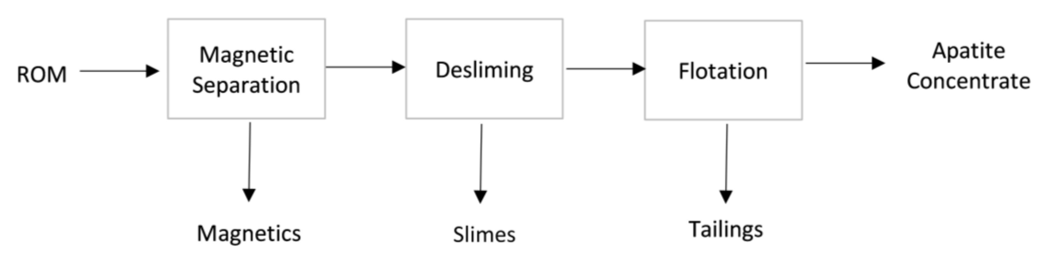
Understanding the relationship between independent and dependent variables requires knowledge of the mineral processing plant’s flowsheet (Figure 1). All geometallurgical samples were submitted to batch tests that mimicked the flowsheet: starting with a magnetic separation step, followed by desliming and flotation.

Magnetics, limes, tailings, and apatite concentrate are plant products. Therefore, each batch test generated the relative fraction of the initial mass destined for each product, making it possible to calculate the yield corresponding to each plant output. In this paper the term “yield” was used to express the ratio between weight or throughput of a stream and the throughput of the plant feed [56,57]. The term “recovery” was used to express the fraction of apatite recovered in a stream with respect to the feed stream.

Let Q_stream represent the solids flowrate of a given stream. Let Y_stream represent the yield of a given stream, then Equations (1) to (4) follow.

$$Y_{Magnetics}=\frac{Q_{Magnetics}}{Q_{ROM}}$$

(1)

$$Y_{Slimes}=\frac{Q_{Slimes}}{Q_{ROM}}$$

(2)

$$Y_{Concentrate}=\frac{Q_{Concentrate}}{Q_{ROM}}$$

(3)

$$Y_{Tailings}=\frac{Q_{Tailings}}{Q_{ROM}}$$

(4)

Thus, four yield values were available (totalling 100%): magnetics, slimes, concentrate, and tailings yield.

Chemical analysis is routinely carried out for the ROM, the flotation feed, and the flotation concentrate streams of the batch tests. The grades in the flotation tailings stream can be calculated from the measured grades in the flotation feed and concentrate streams. The grades in the combined magnetics and slime streams can be calculated using the grades and yields measured in the ROM and in the flotation feed. Let the metallurgical recovery of P₂O₅ in any stream be R_Stream and the grade of P₂O₅ in any stream be g_Stream. The metallurgical recoveries of P₂O₅ were calculated using the yields and grades as shown in Equations (5) to (7). Considering all output points with chemical information (calculated or analysed), it is possible to determine the P₂O₅ metallurgical recovery with respect to the ROM P₂O₅ content, as presented in Equations (6) to (8). It should be noted that when these three variables are added, the result equals 100%, as should be the case with the yield variables.

$$R_{Slimes+Magnetics}=\left(Y_{Slimes}+Y_{Magnetics}\right)\times \frac{g_{Slimes+Magnetics}}{g_{ROM}}$$

(5)

$$R_{Concentrate}=Y_{Concentrate}\times \frac{g_{Concentrate}}{g_{ROM}}$$

(6)

$$R_{Tailings}=Y_{Tailings}\times \frac{g_{Tailings}}{g_{ROM}}$$

(7)

Therefore, the dependent variables to be modeled are the slimes, magnetics, concentrate, and tailings yields, as well as the metallurgical recoveries in the slime + magnetic, in the flotation concentrate, and the flotation tailings.

Table 3. Dependent variables descriptive statistics. Values in %.

Variable (%)	N	Mean	Std. Dev.	Minimum	Q1	Median	Q3	Maximum
YSlimes	3056	42.85	10.10	4.09	36.07	42.37	49.52	81.62
YMagnetics	3056	10.79	8.09	0.04	4.74	9.25	14.95	68.35
YConcentrate	3056	13.74	6.94	0.34	8.47	13.14	18.10	52.55
YTailings	3056	32.61	11.86	1.91	23.19	32.17	41.52	68.84
RSlimes+Magnetics	3056	34.81	10.25	1.86	28.02	33.93	41.11	82.51
RConcentrate	3056	47.81	16.28	0.68	36.99	49.98	60.20	92.08
RTailings	3056	17.38	13.29	0.00	7.20	13.30	24.69	75.10

presents the descriptive statistics for all dependent variables under study. On average, 47.81% of all P₂O₅ and 13.74% of all mass fed in the plant are destined for the flotation concentrate.

2.3. Database Partition

Twenty percent of the samples were randomly selected and set apart to be used as a test set to evaluate the model’s performance. All models presented were elaborated using the remaining 80% of the samples in the database. The k-fold technique [29] was used to determine the optimum parameters for each proposed model. Then, the models obtained were applied to the test dataset.

3. Materials and Methods

The methodology proposed in this work was based on two main methods: artificial neural network (ANN) and recursive feature elimination, both belonging to the machine learning framework.

As explained before, RFE is a technique used in, so-called, ‘Feature Engineering’ aimed at identifying the most relevant input variables to predict either one or a set of output variables. The goal is to use the least possible number of variables, thus simplifying the model while maintaining good accuracy in the predictions.

ANNs are computing systems designed to most efficiently map the relationships between input and output variables in complex structures. These two subjects are more extensively described in the following sections, and the overall methodology can be outlined as follows:

(1)

Selection of the most relevant input variables using RFE;

(2)

The construction of ANN models to predict metallurgical attributes using the input variables selected in the previous step;

(3)

Checking the performance of the built model by forecasting the test dataset.

3.1. Recursive Feature Elimination

As already mentioned, one must decide how many variables will be used as inputs in the prediction model. It is common for the geometallurgical dataset to contain data that is either redundant or not relevant to the prediction of the process performance. Recursive feature elimination (RFE) [28] is an algorithm for automatic feature selection that uses a prediction algorithm in its core to rank the inputs by relevance using a predefined metric. The process starts by creating a predictive model with all the information, organizing the information, and measuring model performance. The less critical predictor is removed at each step. The model is rebuilt iteratively until the desired set of inputs is achieved.

Here, the most relevant subset was found using the RFE version with cross-validation (RFECV) [58], partitioning the dataset tenfold, three times (ten-fold validation with three repetitions). Three different machine learning multitarget predictive models were used in its core: linear regression [59], random forest [60], and CatBoost regressor [61], which will be briefly explained below.

Linear regression is one of the most commonly used techniques for building geometallurgical models [15]. Its goal is to find the equation which minimizes the prediction’s mean squared error using ordinary least squares. To rank the variables for importance, the recursive feature elimination uses the p-value of each variable, removing the one corresponding to the higher p-value in each algorithm iteration, until only the variable with the smallest p-value remains.

The random forest algorithm establishes cutoffs in the input variables, which help to estimate the output variables under study. The greater the number of times an input variable is selected to best describe the output, the greater its importance in the model’s creation. This importance is used inside the RFE to rank the input variables.

The CatBoost algorithm was developed based on the decision trees and gradient boosting theory. The main idea of boosting is to sequentially combine many weak models (small decision trees). Because gradient boosting fits the decision trees sequentially, the fitted trees will learn from former trees’ mistakes and reduce the errors. Adding a new function to the existing ones is continued until the selected loss function is no longer minimized [61]. Similar to other decision tree-based algorithms, CatBoost uses feature importance to rank the relevance of all inputs for the model being created.

It should be noted that only techniques which present a measure of variables’ importance can be used in RFE. Artificial neural networks, ACE [62], and others which do not provide this kind of information, cannot be used in combination with the recursive feature elimination.

To evaluate the performance of each model built, the following metrics were chosen: mean absolute error (MAE), square root of the mean squared error (RMSE), mean absolute percentage error (MAPE), median absolute percentage error (MdAPE), and the Pearson correlation coefficient. Once this study dealt with multitarget models, the mean value of each variable metric was taken to give a general idea of the model’s precision and accuracy. For example, the MAE value was calculated for each of the seven output variables under study. The mean of the seven MAE values was then calculated and this was named the global MAE. The same procedure was used for the other metrics.

The feature selection process was developed in three stages. First, the three predictive algorithm performances were evaluated with RFECV for each subset of relevant inputs in decreasing order until only the most important variable remained, obtaining the global MAE value in each algorithm step. The lowest global MAE value indicated the best predictive algorithm and optimum subset size.

In the second stage, the algorithm selected previously was used inside the RFECV, and the global MAPE for the optimum set was calculated, this being the reference value. All subsets of the variables were analysed (with a lower number of variables than the best case), which provided a global MAPE increase of a maximum of 5%, compared with the reference value. Thus, the smallest subset within the percentage cut-off was chosen as the optimum subset.

In the final third stage, to highlight the importance of the features, an adaptation of the SHAP-values algorithm [63] was used to show the importance of each variable as percentage values.

After the feature selection step, the development of two neural networks started: the first one using the optimum set of variables as inputs (in this case, all available variables) and the second using the variables contained in the optimum subset as inputs. Using this technique to achieve the forecast models was preferred to the CatBoost algorithm, once the neural network results were comparable to the CatBoost results while presenting the advantage of providing the yields and metallurgical balances between the forecasts. Details about the artificial neural network technique are given below.

3.2. Artificial Neural Networks

The artificial neural network technique (ANN) is versatile in geometallurgical model construction. This method can forecast variables with nonlinear relationships with the input parameters, such as the yields and metallurgical recoveries. Additionally, it can simultaneously predict two or more dependent variables using one single network structure. Due to these characteristics and a history of good results [12,14,15], ANN was chosen to predict the geometallurgical responses studied herein. A brief description of the theory related to ANN is given below. For more details about neural networks, their mathematics, and their applications in the mining industry, the reader should refer to Niquini and Costa [14].

Determining which, and how many, variables should be used as inputs is necessary, given that different structures will lead to different results. The independent variables in neural networks are named “input variables” (represented by X), while the dependent variables are named “output variables” (represented by Y). Therefore, the oxide grades in the ROM and the collector dosage inserted in the flotation tests are information that can be used as inputs. The yields and metallurgical recoveries are in the network outputs.

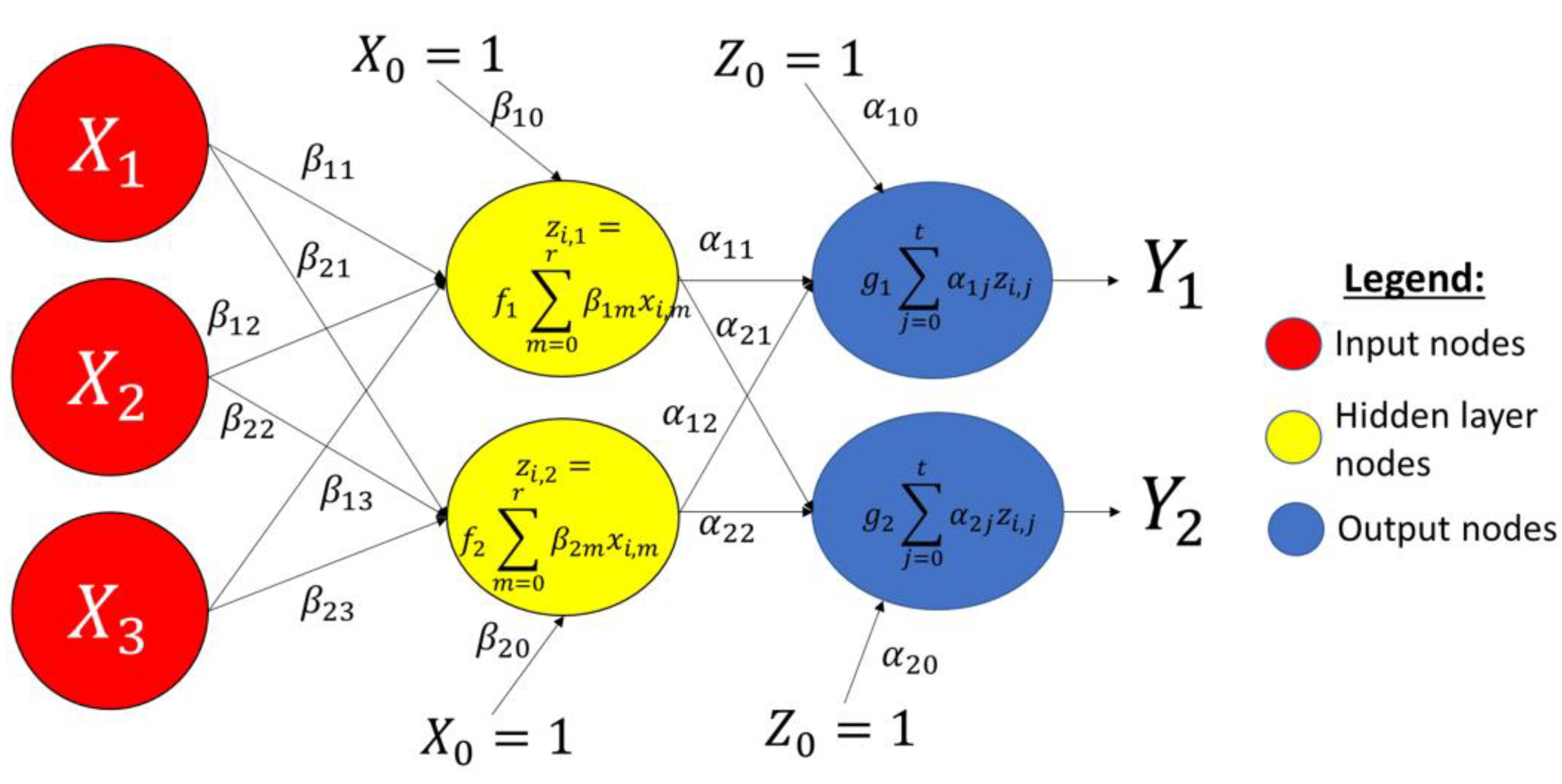
In addition to the input and output layers, there are three other fundamental structures in the ANN: the hidden layer(s), the network weights, and the activation functions (Figure 2).

The user determines the number of hidden nodes and the number of hidden layers. The hidden layer is the intermediary part of the network, where the intermediate calculation to generate the network’s final forecast is carried out. Each hidden node is denoted by Z.

The lines that connect the input layer to the hidden layer and the hidden layer to the output layer are named network weights. They determine the nodes with a greater or a lesser influence in each output node forecast: the higher the weight (in absolute terms), the more significant the influence of the related node, and vice-versa. The determination of α and β weight is usually made using the backpropagation algorithm (details in [64]). Equation (8), an adaptation of the notation given by Izenman [64], shows the position of the weights inside the network forecast function.

$${\widehat{y}}_{i,k}=g_k\left({\sum }_{j=0}^t{\alpha }_{kj}\left(f_j\left({\sum }_{m=0}^r{\beta }_{jm}{x}_{i,m}\right)\right)\right)$$

(8)

where i refers to the sample number in the database, with i = 1, …, n (where n is the total number of samples); k is the index which represents the output variable under study, with k = 1, …, s (where s is the number of output nodes); j is the index which represents the hidden nodes, with j = 0, …, t (where t is the total number of hidden nodes); and m represents the input nodes, with m = 0, …, r (where r is the total number of input nodes in the network).

The functions g and f, in Equation (8), and shown in Figure 2, are the activation functions: a set of predetermined functions which are fed with the linear combination of the input nodes (x) and its β weights, in the case of the f function, or fed with the linear combination of the hidden nodes (z) and its α weights, in case of the g function. Of all the activation functions that exist in the literature, the following were used in this study:

Linear function:

$$\phi \left(v\right)=v$$

(9)

Sigmoid function:

$$\phi \left(v\right)=\frac{1}{1+e^{\left(-v\right)}}$$

(10)

ReLU function:

$$\phi \left(v\right)=max\left(0,v\right)$$

(11)

Softplus function:

$$\phi \left(v\right)=ln\left(1+e^v\right)$$

(12)

Tanh function:

$$\phi \left(v\right)=\frac{(e^v-e^{-v})}{(e^v+e^{-v})}$$

(13)

Using Equation (8) and the activation functions mentioned above, it is possible to forecast the geometallurgical variables of interest. The models can predict the processing plant performance in each block of the 3D block model, aiding in routine mine scheduling procedures.

4. Results and Discussion

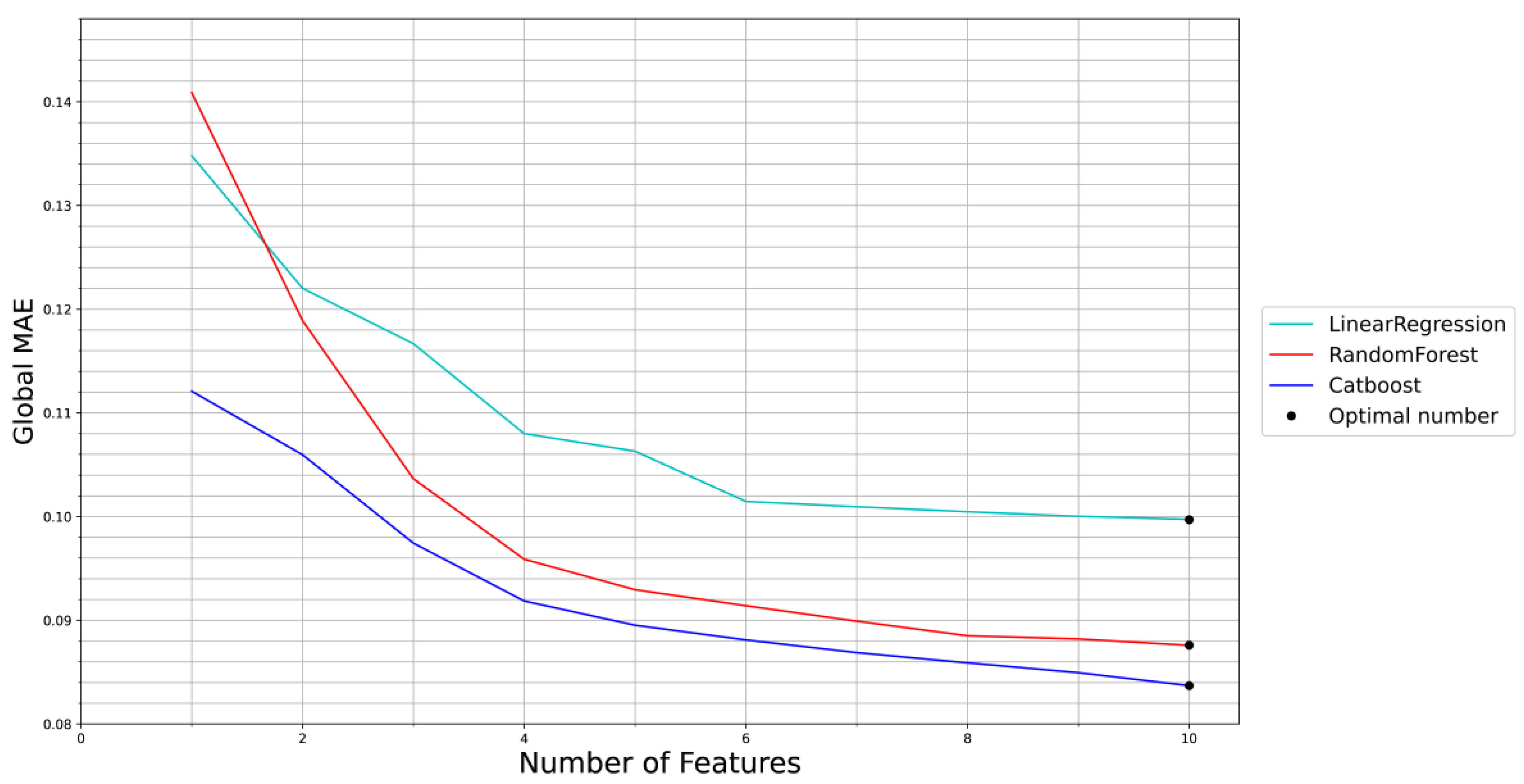
The first step in elaborating the forecast model for the seven output variables consisting of yields and recoveries, was to determine which input variables would be used in the neural network. Following the methodology proposed, the first stage included finding the best predictive algorithm and subset size. Figure 3 presents the performance of the three algorithms for a different number of features. As can be seen, the CatBoost Regressor algorithm is the best for any quantity of inputs, with an optimal performance being achieved by using 10 features in this scenario. Figure 3 also shows that the global MAE presents a lower rate of decrease from four or more inputs. Hence, it is necessary to analyse whether the size reduction of any chosen subset will significantly affect the model’s performance and which variables are selected in each scenario.

The CatBoost algorithm was applied for the optimum set of variables (10 features) and for the subsets containing four to nine features to reduce model complexity. The results for four, five, and six features are presented due to their importance. A ten-fold cross-validation technique was used, considering different randomly selected seeds. The global MAPE value was calculated for each set size, as presented in

Table 4. Global MAPE values observed for the differing number of input variables.

Metric	Catboost Algortithm with
	10 Variables	6 Variables	5 Variables	4 Variables
Global MAPE	6.07	6.36	6.50	6.75

. The increase in the global MAPE value, compared to the best case, is presented in

Table 5. Increase in global MAPE when subsets of variables were used.

Scenario	Catboost Algortithm with	Increase In Global MAPE (%) Compared Agaist the Best Case
1	6 variables	4.6
2	5 variables	7.1
3	4 variables	11.1

.

By analyzing the results, it is possible to conclude that, by choosing the six most relevant features, the global MAPE increment is lower than 5% when comparing this metric against the global MAPE obtained for the best case. Thus, the scenario using six variables was chosen to continue the study.

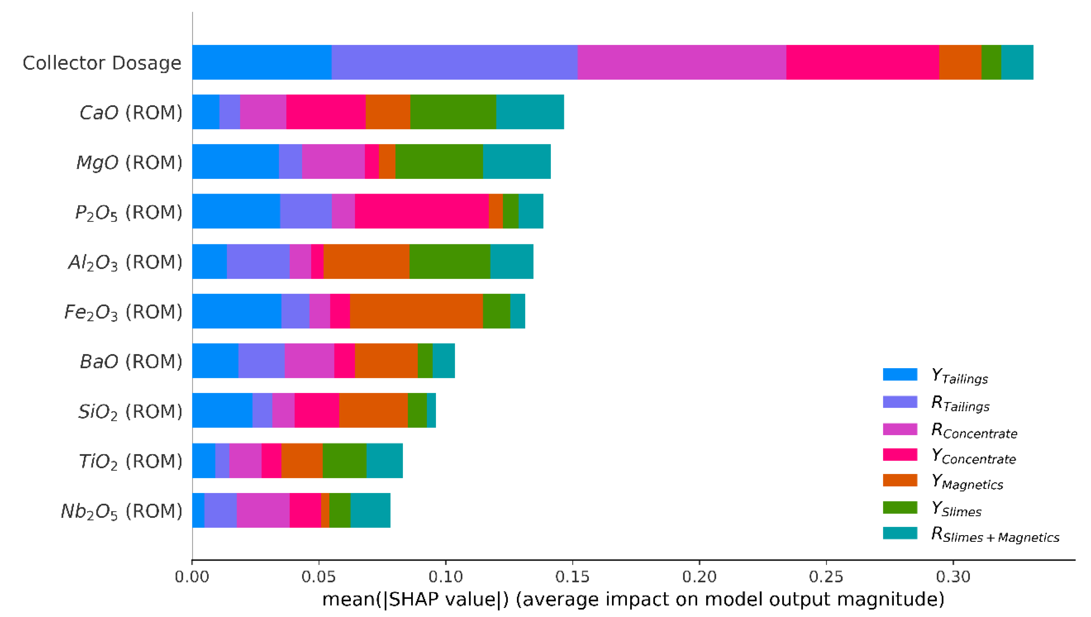
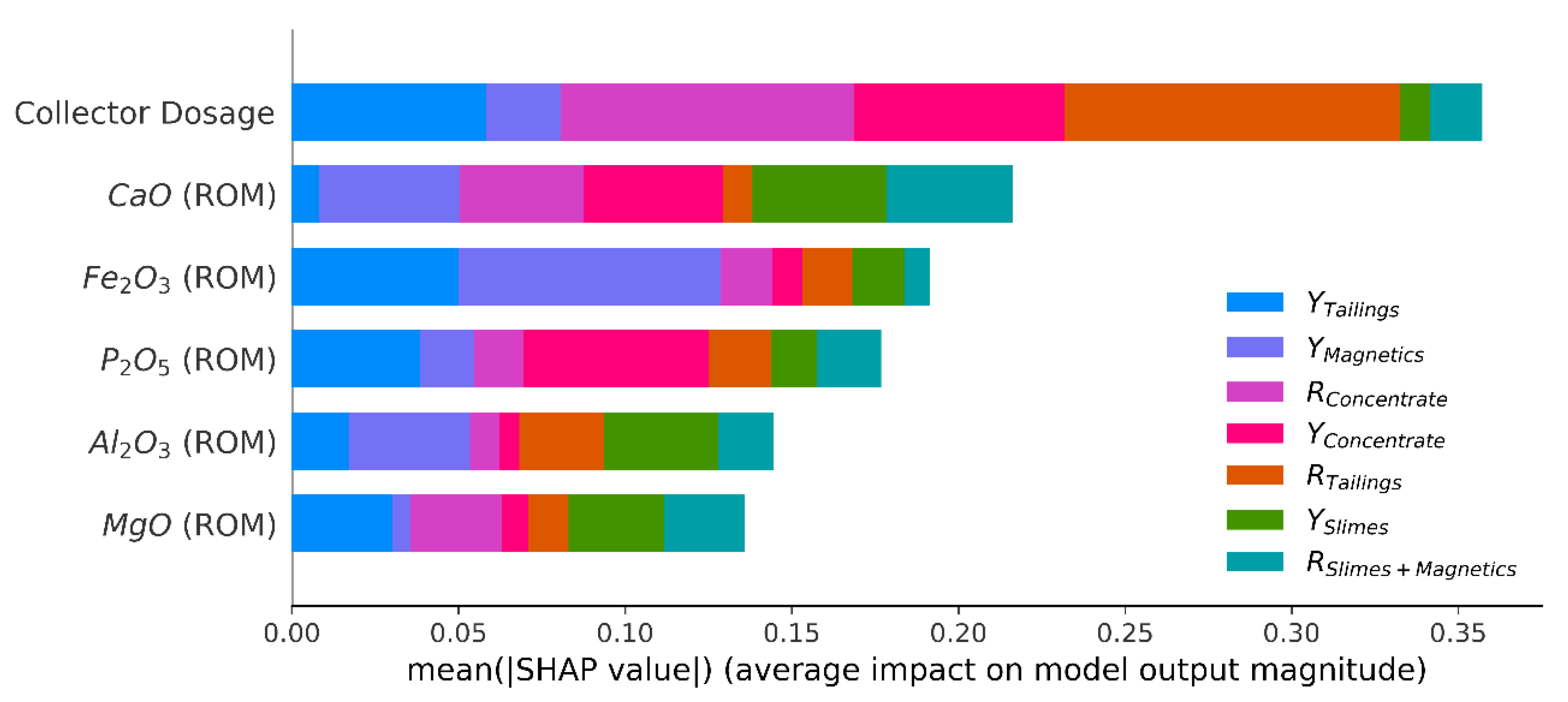
In the next step of the analysis, the CatBoost hyperparameters were calibrated for the two sets of variables: the best one, with all variables available, and the second, with six variables chosen in the reduced scenario. The SHAP-values algorithm was then used to estimate each input variable’s importance (at percentage levels) in both scenarios. Figure 4 illustrates the importance of the optimum scenario (10 features), while Figure 5 presents this information for the subset with six variables. The graphics generated by the algorithm can be interpreted as follows: the X axis represents the importance of each feature to the model (the higher the value, the more important the feature), while the Y axis shows the input variables included in the evaluation. The horizontal bar colors are related to the output variables that are to be predicted (the larger is the color bar, more important the feature is to forecast the respective output behavior). More details about the SHAP values technique can be read in [65].

Amongst the grades, the most important feature to describe the geometallurgical variables was the CaO concentration in the ROM, followed by the MgO concentration in the best scenario and Fe₂O₃ concentration in the sub-optimum scenario. The importance of collector dosage is notorious in both scenarios; being even more important to forecast the flotation concentrate and the tailings recoveries. It is known that the collector dosage cannot influence the desliming and demagnetization processes; thus, the influence of this variable on the yield of slimes, the yield of magnetics and the recovery of slimes + magnetics presented in Figure 4 and Figure 5, are related to a cross-relation with other variables, for example: if the sample has a lot of apatite grains with magnetite, part of the magnetic material will be concentrated in the magnetic separator which will present a high yield, but another part of the apatite grains with magnetite will follow through to flotation. When entering in the flotation step, the laboratory technician will see the apatite grains with magnetite in the sample and will add a higher collector dosage, in order to improve the flotation behavior. Thus, the collector dosage was correlated with the magnetic mass yield not because the first affected the latest, but because the first was calibrated to deal with the characteristic of the sample not concentrated in the magnetic separation step.

BaO, Nb₂O₅, SiO₂ and TiO₂ grades were the variables removed in the reduced scenario. It is known that barite and pyrochlore, the minerals that carry BaO and Nb₂O₅, are present in the deposit and they may affect flotation when their grades are significant; more specifically the barite which competes for the collector of apatite in flotation. Because these minerals are not usually present in high quantities, their influence in the global scenario is reduced, so the grades of BaO and Nb₂O₅ can be removed. The TiO₂ grade was probably selected for removal by the algorithm because it is correlated with the other two variables that were kept in the model (correlation of 0.48 with Fe₂O₃ and 0.46 with MgO). The same occurred with SiO₂, which is correlated with the grades of Fe₂O₃ (0.68), P₂O₅ (0.56) and MgO (0.53).

Next, the neural network’s hyperparameters were calibrated, starting with the complete model with the optimum set of variables, presented in Figure 4. Several tests were carried out to identify the best learning rate [66] to adjust this neural network, and the value found was 0.001. One thousand epochs were used. Two hidden layers were used: the first one with eight hidden nodes and a softplus activation function and the second with nine hidden nodes and a linear activation function. The linear activation function was used in the output layer. These sets of hyperparameters were selected because they provided the smallest global MAE for the validation set. The metrics generated by this network are summarized in

Table 6. ANN metrics using 10 input variables.

Variable	Set	Mean ± Std. Error
		Correlation	MAE	RMSE	MdAPE
YConcentrate	Training	0.854 ± 0.001	2.664 ± 0.013	3.599 ± 0.013	14.938 ± 0.2
YSlimes		0.608 ± 0.002	6.241 ± 0.021	8.042 ± 0.033	12.297 ± 0.067
YMagnetics		0.855 ± 0.001	3.05 ± 0.013	4.156 ± 0.015	25.445 ± 0.16
YTailings		0.837 ± 0.001	5.158 ± 0.036	6.534 ± 0.035	13.711 ± 0.077
RConcentrate		0.667 ± 0.002	9.296 ± 0.036	12.174 ± 0.044	14.564 ± 0.17
RSlimes+Magnetics		0.456 ± 0.002	6.964 ± 0.016	9.149 ± 0.022	16.155 ± 0.048
RTailings		0.688 ± 0.001	6.941 ± 0.031	9.596 ± 0.022	36.768 ± 0.231
YConcentrate	Validation	0.849 ± 0.008	2.708 ± 0.06	3.641 ± 0.082	15.482 ± 0.473
YSlimes		0.585 ± 0.017	6.35 ± 0.078	8.272 ± 0.134	12.239 ± 0.233
YMagnetics		0.847 ± 0.009	3.115 ± 0.067	4.28 ± 0.135	25.999 ± 0.727
YTailings		0.83 ± 0.006	5.24 ± 0.077	6.664 ± 0.09	13.909 ± 0.26
RConcentrate		0.655 ± 0.014	9.432 ± 0.208	12.291 ± 0.253	14.774 ± 0.416
RSlimes+Magnetics		0.435 ± 0.017	7.059 ± 0.136	9.236 ± 0.18	16.348 ± 0.644
RTailings		0.676 ± 0.013	7.065 ± 0.191	9.728 ± 0.191	37.596 ± 1.316
YConcentrate	Test	0.866	2.631	3.601	14.897
YSlimes		0.583	6.389	8.416	12.449
YMagnetics		0.837	3.276	4.602	27.851
YTailings		0.833	5.353	6.741	14.263
RConcentrate		0.625	9.479	12.843	13.925
RSlimes+Magnetics		0.424	7.073	9.276	16.199
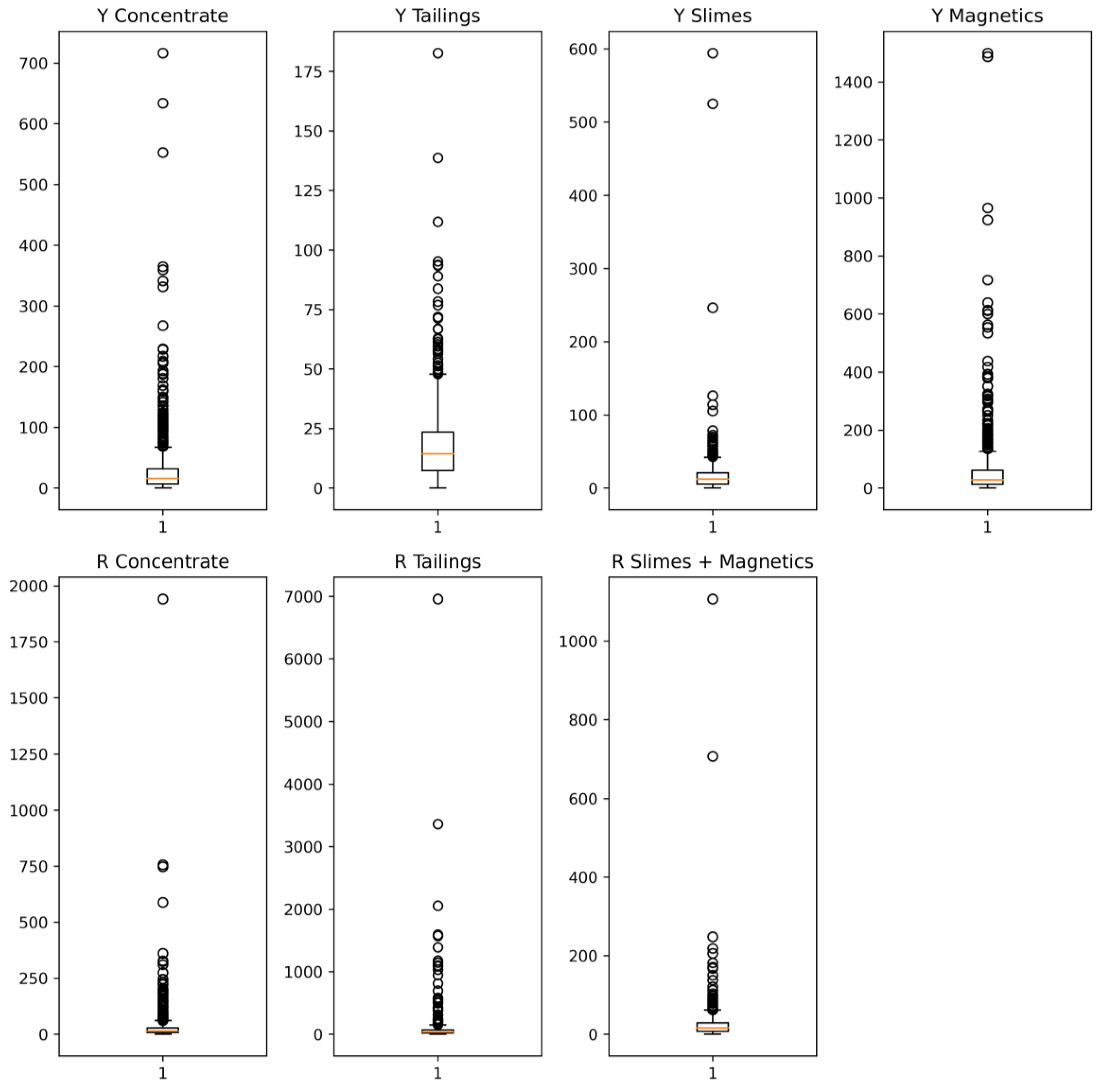
RTailings		0.658	7.181	10.420	34.133

. The first value in each cell represents the metric mean of the ten-fold validation, and the second represents the standard error. At the bottom of the table, the test set results obtained when the training and validation sets are combined to create the final model are presented. The MdAPE metric was selected to be analyzed because the outliers (illustrated in Figure 6) inflated the mean absolute percentage error (MAPE), which may lead to an erroneous model interpretation.

The correlation coefficient between the forecasts and the real values for the flotation concentrate yield was 0.866, and the MdAPE found was 14.897 in the test set. For the flotation concentrate P₂O₅ recovery, the correlation coefficient was 0.625, associated with a MdAPE value of 13.925. The slimes yield and the slimes + magnetics P₂O₅ recoveries also showed good MdAPE values (12.449 and 16.199, respectively), although the correlation coefficient between the real values and the forecasts is not very high. The magnetics yields and tailings P₂O₅ recovery were the variables with the highest MdAPE values (27.851 and 34.133, respectively).

After completing the analysis with the optimum scenario, the neural network’s calibration was conducted using the six variables presented in Figure 5. Two hidden layers were used: the first with 10 hidden nodes and a sigmoid activation function and the second with 10 hidden nodes and a linear activation function. The linear activation function was used in the output layer. The best learning rate found to adjust this network was 0.002 and one thousand epochs were used. The metrics generated by using this network are summarized in

Table 7. ANN metrics using six input variables.

Variable	Set	Mean ± Std. Error
		Correlation	MAE	RMSE	MdAPE
YConcentrate	Training	0.855 ± 0.001	2.664 ± 0.025	3.598 ± 0.018	15.122 ± 0.32
YSlimes		0.599 ± 0.001	6.334 ± 0.022	8.093 ± 0.021	12.523 ± 0.062
YMagnetics		0.846 ± 0.001	3.195 ± 0.019	4.319 ± 0.018	26.523 ± 0.149
YTailings		0.835 ± 0.001	5.165 ± 0.021	6.528 ± 0.025	13.692 ± 0.072
RConcentrate		0.667 ± 0.002	9.32 ± 0.069	12.221 ± 0.06	14.601 ± 0.302
RSlimes+Magnetics		0.463 ± 0.002	6.957 ± 0.02	9.121 ± 0.031	16.231 ± 0.082
RTailings		0.692 ± 0.002	6.902 ± 0.055	9.561 ± 0.028	36.608 ± 0.457
YConcentrate	Validation	0.851 ± 0.008	2.706 ± 0.056	3.634 ± 0.075	15.564 ± 0.346
YSlimes		0.582 ± 0.012	6.412 ± 0.065	8.205 ± 0.092	12.732 ± 0.23
YMagnetics		0.84 ± 0.007	3.225 ± 0.073	4.372 ± 0.098	26.718 ± 0.788
YTailings		0.829 ± 0.006	5.236 ± 0.071	6.629 ± 0.097	13.855 ± 0.281
RConcentrate		0.657 ± 0.012	9.385 ± 0.207	12.32 ± 0.261	14.674 ± 0.404
RSlimes+Magnetics		0.447 ± 0.017	7.002 ± 0.135	9.168 ± 0.181	16.463 ± 0.276
RTailings		0.682 ± 0.011	6.985 ± 0.133	9.659 ± 0.174	36.91 ± 0.964
YConcentrate	Test	0.859	2.671	3.650	16.169
YSlimes		0.586	6.470	8.437	12.656
YMagnetics		0.838	3.312	4.599	28.397
YTailings		0.827	5.490	6.854	14.806
RConcentrate		0.634	9.395	12.637	15.157
RSlimes+Magnetics		0.443	7.006	9.191	16.189
RTailings		0.665	7.244	10.233	34.327

.

The results presented in Table 7 show that for the reduced set of input variables, the metrics observed were very similar to the ones seen in the optimum scenario, especially for the variables with the most significant economic impact, namely the flotation concentrate yield and P₂O₅ recovery.

Using six and 10 features, a comparison of the two scenarios can be summarized by calculating the relative differences, as shown in Equation (14).

Table 8. Relative differences between the sub-optimum scenario and the optimum.

Variable	Set	Relative Difference (%)
		Correlation	MAE	RMSE	MdAPE
YConcentrate	Training	0.1%	0.0%	0.0%	1.3%
YSlimes		−1.5%	1.5%	0.6%	1.9%
YMagnetics		−1.1%	4.8%	3.9%	4.2%
YTailings		−0.2%	0.1%	−0.1%	−0.1%
RConcentrate		0.0%	0.3%	0.4%	0.3%
RSlimes+Magnetics		1.5%	−0.1%	−0.3%	0.5%
RTailings		0.6%	−0.6%	−0.4%	−0.4%
YConcentrate	Validation	0.2%	−0.1%	−0.2%	0.5%
YSlimes		−0.5%	1.0%	−0.8%	4.1%
YMagnetics		−0.8%	3.5%	2.1%	2.8%
YTailings		−0.1%	−0.1%	−0.5%	−0.4%
RConcentrate		0.3%	−0.5%	0.2%	−0.7%
RSlimes+Magnetics		2.8%	−0.8%	−0.7%	0.7%
RTailings		0.9%	−1.1%	−0.7%	−1.8%
YConcentrate	Test	−0.7%	1.5%	1.4%	8.5%
YSlimes		0.3%	1.3%	0.3%	1.7%
YMagnetics		0.1%	1.1%	−0.1%	1.9%
YTailings		−0.7%	2.6%	1.7%	3.8%
RConcentrate		1.4%	−0.9%	−1.6%	8.8%
RSlimes+Magnetics		4.5%	−1.0%	−0.9%	−0.1%
RTailings		1.1%	0.9%	−1.8%	0.6%

summarizes the relative differences observed between the Pearson correlation coefficients, MAE, RMSE, and MdAPE mean values.

$$Relative Difference=\left(\frac{{Metric Value}_{6features}-{Metric Value}_{10features}}{{Metric Value}_{10features}}\right)\ast 100\%$$

(14)

By analysing the relative difference in the test set, it is possible to conclude that when the correlation coefficient decreases, the fall is not marked (smaller than 0.7%), showing that the reduction in the number of input variables did not impact the model’s precision. In most cases, an improvement in the correlation coefficient value is noted when the reduced set of variables is used.

Removing four variables from the inputs did not significantly affect the metrics. The relative differences in the MAE and RMSE values showed an increase in errors lower than 2.6% when the reduced set of variables is used instead of the optimum set. The most significant impact observed was in the MdAPE values for the flotation concentrate mass and metallurgical recoveries, showing an increase of 8.5% and 8.8% in the test set, respectively, when the reduced scenario was adopted. The reduced model can be considered as a good option to forecast the metallurgical variables of interest because the MdAPE increase was lower than 4% for all other output variables.

Considering the above results, it can be concluded that it is possible to work with the reduced model without losing much, in terms of model precision and accuracy. There is a gain in simplicity once adding variables in the process can represent a considerable increase in the workload, not only in computer power but also in time spent by the analyst to elaborate, update, and evaluate the models created to estimate the input variables in the block model using kriging or simulation. Analysing through the geostatistical point of view, passing from 10 to six variables to be modelled implies a work-time reduction of 40%, a considerable amount.

5. Conclusions

Reducing the number of variables leads to a lower computational cost. The gain is also felt in the geostatistical workflow, once the number of input variables to be integrated to the resource block model is reduced. However, those benefits are counterbalanced by higher errors in the forecasting of some variables. The trade-off between a small error and a higher labor force is important when applying such models to a complete industrial operation. To help with this decision, it is important to quantify the errors related to the two approaches and compare them, as shown in this paper.

In this case study, the reduction from 10 to six input variables showed that dimension reduction can lead to models capable of returning correlation values close to the ones observed when the complete set of variables is used, with a small loss in the reduced scenario, when it occurs. The increase in MAE and RMSE was smaller than 2.6% for all output variables in the test set when the sub-optimum set of variables was used instead of the set with all 10 features. The four removed variables make sense considering the points discussed in chapter 4: the BaO and Nb₂O₅ are related to the presence of barite and pyrochlore, which only affects the process in high quantities (which is rare); and SiO₂ and TiO₂ grades are correlated with other variables that were maintained in the model, making their presence redundant. Thus, it was decided to select the model elaborated with the reduced number of input variables, due to its quality, and considering the practicality of the whole process, as this is a workflow being suggested for an active mining operation where time response represents a crucial aspect.

We would like to stress that each case study is unique. It is possible to achieve smaller errors in the test set with a reduced set of variables compared with the optimum scenario, especially if small datasets are used, due to overfitting (caused by a high number of variables and a small number of samples). It is also possible to find higher errors that do not justify the dimensionality reduction. Thus, it is important to follow the proposed workflow and analyze the errors in both scenarios to choose the best option for each mine under study.

It is important to mention that the geometallurgical ore model herein described is essentially statistical in nature. Nevertheless, the model is powerful enough to include some of the physical–chemistry aspects of the process. For example, the properly carried out investigation has led to the establishment of a quantitative relationship describing the deleterious effect of the presence of carbonates in the plant’s feed, understood as the ratio between CaO and P₂O₅, proving that important geochemical/mineralogical relationships were mathematically predicted, giving an interpretation of the results that makes geological sense.

Another important point that needs to be stressed is related to the estimation of the collector dosage in the block model. In this case study, this explanatory variable was attributed to the blocks by the nearest neighbor estimation method. Thus, mining regions which require a smaller collector dosage can be recognized, and areas which demand a higher collector dosage are also noted.

Final Thoughts about Mineral Processing

Usually, the processing plant’s human operator(s) has a well-established objective of a certain number of tonnes of the product (concentrate) with a required grade or quality. Such quality may include different grades (for example, SiO₂ and Fe₂O₃, but most certainly P₂O₅). A conveyor belt equipped with a scale provides the tonnage of the filtered product, so this information is readily available through the control system. At short time intervals, samples are taken and sent for analysis so that, given a short delay, product quality and moisture content are also available to the operator. Given that the plant is operating at a steady pace, the operator may decide to change the processing parameters so that the production objectives are met during his shift. The changes that can be made are relatively small, such as in the reagent dosage, aeration rate, and perhaps also the froth levels, and froth-wash-water flowrate.

The point here is that most of the plant’s processing parameters do not change at all, and for the few parameters that do change, so that production requirements can be met, the impacts on the production rate and quality are well-known. Therefore, it is safe to assume that the plant and all its processing parameters can either be changed to meet the required quality or not. Simply put, if the quality can be met, the rock is ore, and if not, the rock is waste. The broad question that is left concerns the metallurgical recovery of P₂O₅ as a function of ore quality. In other words, for the development of the geometallurgical model, the main concern is with the ore model.