Machine Learning Model of Hydrothermal Vein Copper Deposits at Meso-Low Temperatures Based on Visible-Near Infrared Parallel Polarized Reflectance Spectroscopy

Abstract

The verification efficiency and precision of copper ore grade has a great influence on copper ore mining. At present, the common method for the exploration of reserves often uses chemical analysis and identification, which have high costs, long cycles, and pollution risks but cannot realize the in situ determination of the copper grade. The existing scalar spectrometric techniques generally have limited accuracy. As a vector spectrum, polarization state information is sensitive to mineral particle distribution and composition, which is conducive to high-precision detection. Taking the visible-near infrared parallel polarization reflectance spectrum data and grade data of a copper mine in Xiaoyuan village, Huaining County, Anhui Province, China, as an example, the characteristics of the parallel polarization spectra of the copper mine were analyzed. The spectra were pretreated by first-order derivative transform and wavelet denoising, and the dimensions of wavelet denoising spectra, parallel polarization spectra, and first-order derivative spectra were also reduced by principal component analysis (PCA). Three, four, and eight principal components of the three types of spectra were selected as variables. Four machine learning models, the radial basis function (RBF), support vector machine (SVM), generalized regression neural network (GRNN), and partial least squares regression (PLSR), were selected to establish the PCA parallel polarization reflectance spectrum and copper grade prediction model. The accuracy of the model was evaluated by the determination coefficient (R²) and root mean square error (RMSE). The results show that, for parallel polarization spectra, first-order derivative spectra, and wavelet denoising spectra, the PCA-SVM model has better results, with R² values of 0.911, 0.942, and 0.953 and RMSE values of 0.022, 0.019, and 0.017, respectively. This method can effectively reduce the redundancy of polarized hyperspectral data, has better model prediction ability, and provides a useful exploration for the grade analysis of hydrothermal copper deposits at meso-low temperatures.

1. Introduction

Hydrothermal vein copper deposits at meso-low temperatures are often produced in neutral, weakly acidic, and alkaline volcanic rocks or shallowly formed intrusive bodies [1]. The natural type of ore is mainly copper-bearing diorite, and the metal minerals are mainly chalcopyrite in the ore, which is relatively high grade, easy to mine and process, and has high metal recovery [2]. As an important indicator of mineral processing, the ore grade and recovery rate is closely related to the level of mineral extract technology. For the different copper grades, the recovery method adopted is not the same. Therefore, how to determine the copper ore grade and mine reserves quickly and accurately at low cost is particularly important. The common method of ore grade determination often uses chemical analysis, such as chemical leaching, magnetic separation, and flotation [3,4,5,6], which is accurate but has a high cost and long determination period and cannot realize instant in situ determination of ore grade. In addition, there is a hysteresis effect relative to the ore allocation process [7,8]. Therefore, how to quickly and accurately determine copper content of copper ore is a difficult problem in mineral processing technology. It is of great significance to reduce costs and quickly apply to the evaluation of copper reserves and potential areas.

In recent years, with the rapid development of hyperspectral measurement technology, hyperspectral quantitative prediction technology has been used in the field of metallic and nonmetallic mineral content or grade detection. This method is with nondestructive detecting, fast detecting speed, high resolution, and low cost [9,10,11]. To extract spectral characteristic information more accurately and quickly, many scholars have carried out in-depth research on modeling methods. Genetic algorithm (GA) and Back Propagation neural network algorithm (BP) were applied to estimate the grade of low-grade porphyry copper deposit. Principal component analysis (PCA) and local linear embedding (LLE) were used to reduce the dimension of original spectral data. The results showed that the average absolute error of grade prediction of the model from the data processed by genetic algorithm was 0.045%, and the accuracy was significantly improved [12,13]. Stepwise multiple linear regression (SMLR) and principal component regression (PCR) were performed to effectively predict the copper content by visible-near infrared and shortwave infrared reflectance spectroscopy in the copper mine. The best and worst prediction performances were obtained by stepwise multiple linear regression (R² = 0.89) and principal component regression (R² = 0.37) methods [14,15,16]. Although some progress has been made in hyperspectral research, there is still no standard algorithm or model for the quantitative prediction of mineral elements and the accuracy of prediction needs to be further improved at present [17]. The main reason is that the ore composition varies, the cross interference of the spectral response of a variety of associated minerals results in the difference in the mineral surface reflectance, and the intensity spectrum is also easily polluted by the skylight [18,19].

As an independent characteristic of electromagnetic radiation, polarization is different from the reflectivity spectrum. It reflects the vibrational state of light interacting with the medium. When nonpolarized natural light enters the atmosphere, the scattering and absorption of the atmosphere will deflect the sunlight. Polarized reflected light will be generated in the mineral surface and bring the polarization state information closely related to the mineral surface physical characteristics [20]. Its change mode and degree are not only closely related to mineral content and surface materials, but also have high correlation with ore particle size, particle shape and distribution, surface roughness, refractive index, etc., which is a unique characteristic that the reflectivity spectrum does not have [21,22]. Therefore, in principle, polarization state information can be a useful supplement to hyperspectral data under the condition of complex mineral composition. It is helpful to improve the predicted accuracy of the hyperspectral model of copper grade [23]. In recent years, the exploration of polarization technology has shown the potential of polarization in the field of geological and mineral resources. An acousto-optical tunable filters (AOTF) spectro-polarimeter was used to obtain polarized reflection information of gypsum and kaolin, which revealed additional information on the mineral spectra by near infrared polarized spectroscopy [24]. A reflected light microscope and a polarizer plate were combined to contrast the unpolarized and polarized images, and an improved regional growth segmentation method was used to identify hematite particles based on reflectivity and texture information, which effectively improved the contrast of mineral particle images [25]. Furthermore, the self-developed polarization measurement system and processing software by Yang, Y.H. et al., were applied to systematically study the polarization spectrum characteristics of 11 common alteration minerals. The results showed that by visible-short wave infrared spectra, fluorite, quartz, potassium feldspar, and other minerals were not easily distinguished, but the polarization spectrum could enhance mineral recognition and classification [26]. In addition, chalcedony, quartz, opal, and calcite were measured with an ISI921VF field spectroradiometer and polarization modulation module, demonstrating that in the laboratory the incidence angle and detection angle of light had a significant impact on the polarization degree spectrum of the ore. Among the samples, chalcedony with small constituent particles and high crystallinity had the strongest polarization characteristics, but the polarization property of amorphous opal was the weakest [27].

The above research shows that vector polarized hyperspectral detection technology can not only obtain the polarized reflected spectral information of minerals but also characterize the vibrational state of light vectors in the process of radiation [28]. However, this information is easily affected by the incident direction of the light source and the observation direction of the sensor, which greatly reduce the predicted accuracy of ore grade [27]. When the light interacts with the mineral surface, the vibration direction is changed. The inhomogeneity of the horizontal and vertical components of the polarized light will generate the intensification of light energy in a certain direction. For example, the parallel polarized light can reduce the contribution of light reflection from the sky, avoid strong background light disturbance, reduce flare pollution, and effectively improve the target contrast for the surface with low reflection radiation intensity. It is helpful to reduce the uncertainty of direction and improve the detection accuracy of copper ore grade [29].

In this study, we aim to provide a novel approach for the rapid and accurate estimation of copper ore grade of hydrothermal copper deposits at meso-low temperatures. The capability of visible-near infrared parallel polarized reflectance spectroscopy will be discussed about detecting the grade of copper ore. To reduce the dimension of the input dataset, PCA will be carried out, and an optimal quantitative prediction model of copper ore grade will be established by comparing the performance of the radial basis function (RBF), support vector machine (SVM), generalized regression neural network (GRNN) and partial least squares regression (PLSR), so as to provide an effective technical means for accurately determining the in situ grades of the copper deposits [30].

2. Materials and Methods

2.1. Study Area and Ore Samples

The mining area is located 20 km northwest of Anqing city, 12 km southeast of Huaining County, and 2 km east of Yueshan town in Anhui Province, China. The mining area covers an area of 7.29 square kilometers and is under the jurisdiction of Xiaoyuan Village, Yueshan Town, Huaining County. The mining area belongs to the Susong Lujiang fault uplift of the Yangtze River fold fault belt in the Yangtze platform depression. The deposit originates from the north wing of the Huangmeishan short axis anticline near the West Branch North contact zone of the Yueshan rock mass, and the exposed strata are Lower and Middle Triassic carbonate rocks and clastic rocks. The mining area is shown in Figure 1a. According to the borehole core as shown Figure 1b, the alteration is mostly veinlet, disseminated veinlet, irregular veinlet, and lump, which is obviously controlled by the contact zone and structural fracture, and is accompanied by veinlet or spotted brass mineralization, magnetite mineralization, and pyritization.

The 66 grade control samples were taken from different percussion drill holes of hydrothermal copper deposits at meso-low temperatures as shown Figure 1b,c. First, they were crushed by an XPC 150 × 125 jaw crusher and a PE 60 × 100 jaw crusher. Then, an RK/PG250 × 150 roller crusher and a single- and double-deck dual-purpose vibrating screen were used to crush samples to less than 1 mm. The ring cone method was used to mix the stacking cone 4 times, and 66 pieces were bagged by reduction sampling with 1000 g each. Next, a XMQ 240 × 90 conical ball mill was used to grind the ore, the ground sample was wet sieved with a 200 mesh standard sieve, and the product on the sieve was dried and then sieved by a dry-type check using a 200 mesh sieve. To obtain the copper power samples, the grinding fineness of less than 0.074 mm was calculated from the weight of the product on the sieve, and the copper ore samples were produced by multiple selection and sweeping.

2.2. The Concept of Parallel Polarized Reflection (PPR)

Polarization is the characterization of a vector wave observed at a fixed point in space as a function of time in terms of vector waves. Polarization of light is a phenomenon in which the spatial distribution of the electric vector vibration of the light wave loses symmetry with respect to the direction of light propagation, and its quantified characterization can be expressed by the Stokes parametric method, as follows [29]:

$$\mathrm{S}=\left[\begin{array}{l}I\\ Q\\ U\\ V\end{array}\right]=\left[\begin{array}{l}{E}_l{E}_l^{*}+E_r{E}_r^{*}\\ E_l{E}_l^{*}-E_r{E}_r^{*}\\ E_l{E}_r^{*}+E_r{E}_l^{*}\\ i(E_l{E}_r^{*}-E_r{E}_l^{*})\end{array}\right]$$

(1)

where I denotes the total intensity of the light wave, Q denotes the difference in intensity of linearly polarized light in the x and y directions, U denotes the difference in intensity of linearly polarized light in the +1/4π and −1/4π directions, V denotes the intensity of circularly polarized light, $E_l$ and $E_r$ are the electric vectors parallel and perpendicular to the reference plane, respectively, and $E_l{}^{*}$ and $E_r{}^{*}$ are the $E_l$ and $E_r$ conjugate matrices, respectively.

The parallel polarized light reflection intensity (L) is

$$\mathrm{L}=I+Q=2E_l{E}_l^{*}$$

(2)

The parallel polarized reflection (PPR) is

$$PPR=\frac{\pi L}{F_0\cos \theta }$$

(3)

where $F_0$ is the solar spectral irradiance, which is obtained by the reference plane in the actual measurement, and $\theta$ is the solar zenith angle [31].

2.3. Data Acquisition and Preprocessing

2.3.1. Measurement of Copper Grade of Ore Samples

By chemical analysis, the copper grade of the 66 samples was obtained. As shown in

Table 1. Descriptive statistics of samples.

Sample Number	Copper Grade (%)
	Min	Max	Mean	Standard Deviation
66	0.01	19.25	7.56	6.51

, the average copper grade of the samples is 7.56%, the highest copper grade of raw ore is 4.23% by core crushing and the copper grade is up to 19.25% by foam flotation.

2.3.2. Measurement of Ore Sample Spectra

An SVC HR-1024 spectrometer was used for spectral measurements, which has a wavelength range of 350~2500 nm, spectral accuracy higher than ±0.5 nm, and FWHM ≦8.5 nm [31]. We installed a polarized lens with an arbitrary rotation angle and a 5° lens diaphragm. The effective wavelength range of the polarizer in the lens was 450 nm–1700 nm. We used a 2000 W photographic spotlight lamp with the illuminance of 39,800 lux per meter as the light source at a 45-degree angle with the horizontal direction and a 10° bare optical fiber probe to receive the polarized reflectivity data. The polarization reflection spectra of ore samples were measured in a dark room. The sample was placed in a 10 cm diameter, 2 cm deep container, and the surface was scraped flat with a ruler and the spectrometer lens was perpendicular to the sample observation surface. During the measurement, the multiangle measuring frame was used for automatic spectral measurement as shown in Figure 2b, and the unbiased and 0°, 60°, and 120° polarized states were selected. Five spectra curves were collected for each sample, and the average reflectance over five tests was taken as the polarized reflectance.

Figure 3 shows the parallel polarized reflection spectrum curve of 66 samples. The spectral characteristics are as follows:

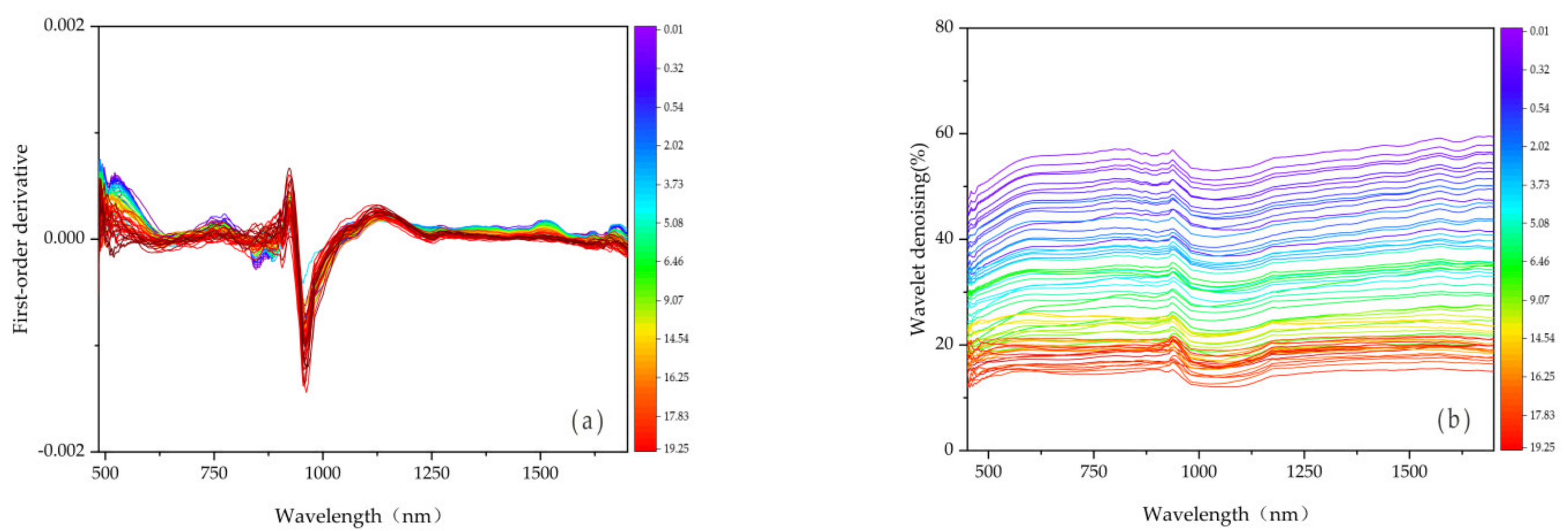
• The parallel polarized reflectivity of the sample spectrum has an obvious spectral discrimination between 10% and 60%. The parallel polarized spectra of different grades have a high degree of separation. With the increase in parallel polarization reflectivity, copper ore grade shows a downward trend. The parallel polarized reflectivity shows a rapid upwards trend at 450–600 nm when the copper content is lower, and a deep trough appears at 1000 nm.
• The spectral curves near 900 nm and 1700 nm show differences with copper content. For the copper grade less than 10%, the polarization reflection curves show a large fluctuation, but the change is gentle when the ore grade is greater than 10%.

2.3.3. Spectral Transform

After spectral acquisition, the spectral data were smoothed by the Savitzky–Golay method to prevent noise from disturbing the experimental results. Then the spectrum was transformed using derivative, wavelet denoising to reduce the influencing factors, such as background environment, illumination, and highlighting the characteristic spectrum of the target.

The derivative algorithm is a common data pre-processing method, and the derivative transformation can eliminate the influence of background information, thus improving the spectral resolution and facilitating the extraction of feature bands [32].

Wavelet denoising adopts the discrete wavelet transform method to preprocess the noisy signal, decompose the signal into various scales, remove the wavelet coefficients belonging to the noise at each scale, retain and enhance the wavelet coefficients belonging to the signal, and then recover the detection signal through the inverse wavelet transform [33].

The spectral curve after the first-order derivative processing is shown in Figure 4a. It can be seen from the figure that three peaks and three valleys are formed. Figure 4b shows that the curve after wavelet transformation has roughly the same trend as the polarization spectrum. Because the spectrum after wavelet denoising can not only effectively filter the noise, but also better retain the useful signal, avoid signal loss, and significantly improve the signal quality.

2.3.4. Spectral Dimension Reduction

In order to reduce the hyperspectral dimension, extract the main spectral features, compress the data, and improve the calculation speed, principal component analysis (PCA) is often used. PCA is a commonly used linear data dimension reduction method, and the extraction of original data is realized through linear changes [34]. It supports a small number of irrelevant variables to describe the data and retains more useful information.

PCA was used to reduce the dimensions of the parallel polarization spectra, first-order derivative spectra and wavelet denoising spectra. The number of principal components with a cumulative contribution rate of 90% is the input variable. The principal components of the parallel polarization spectrum, first-order derivative spectrum and wavelet denoising spectrum are 4, 8, and 3, respectively. The contribution rate of the three spectral principal components is shown in Figure 5.

2.4. Methods

2.4.1. Radial Basis Function Neural Network Model (RBF)

RBF neural network is a three-layer network with a single hidden layer, which is usually divided into an input layer, a hidden layer, and an output layer. Radial basis functions are used as activation functions in the hidden layer, and in this paper, the Gaussian kernel function is chosen as the activation function [35]. Its form is as follows:

$$R(\mathrm{x})=\exp (-{\frac{‖x-c‖}{2{\sigma }^2}}^2)$$

(4)

where x is the input data of sample, c is the kernel function center point, and $\sigma$ is the width parameter of the function. The third layer is the output layer, where the output layer of the network is a linear weighting of the output of each neural unit in the hidden layer.

2.4.2. Generalized Regression Neural Network (GRNN)

GRNN is a modification of the radial basis neural network with a four-layer neural network structure, which is usually divided into an input layer, pattern layer, summation layer, and output layer [36]. GRNN can build generalized regression neural networks by radial basis neurons and linear neurons, which are suitable for applications in function approximation. Radial basis functions and competing neurons can build probabilistic neural networks, which are commonly used to solve classification problems.

2.4.3. Partial Least Squares Regression (PLSR)

PLSR is a multivariate statistical method that is commonly used in hyperspectral models and can be a good solution to the problem of multiple colinearity in independent variables. First, the training set input spectral matrix X and output copper content matrix Y are decomposed by PLSR as follows:

$$X=T{P}^T+E,$$

(5)

$$Y=U{Q}^T+\mathrm{F}$$

(6)

where T and U are the score matrices of matrices X and Y, P and Q are the load matrices of matrices X and Y, and E and F are the residual matrices of X and Y, respectively [37].

During prediction, the score matrix T and U are subject to linear regression, and the form is as follows:

$$U=TB+E_d,$$

(7)

where B and E_d are the matrices of the regression coefficient and residuals, respectively.

2.4.4. Support Vector Machine (SVM)

SVM is a binary classification model that maps feature vectors of instances to certain points in space to solve nonlinear and high-dimensional classification problems by small and medium sample data, and is later extended for solving regression problems, also known as support vector regression [38]. Given a training dataset D = {(x_i, y_i), i = 1, 2, …, n} with n samples, a linear regression function $f(x)=wx+b$ can be built to approximate the target value y_i, assuming the existence of an f(x) that can estimate all the data with ε accuracy, considering the case of fitting errors and introducing relaxation factors ${\xi }_i\ge 0,{\xi }_i^{*}\ge 0,$ the support vector regression problem can be formalized as:

$$\min \frac{1}{2}{‖w‖}^2+C{\displaystyle \sum _{i=1}^n({\xi }_i+{\xi }_i^{*})}$$

(8)

Subject to

$$\left\{\begin{array}{l}{y}_i-w{x}_i-b<\epsilon +{\xi }_i\\ w{x}_i+b-y_i<\epsilon +{\xi }_i^{*}\\ {\xi }_i,{\xi }_i^{*}\ge 0\end{array}\right.$$

(9)

where the constant C > 0 is the penalty factor [39].

The SVM modeling originates from the MATLAB LIBSVM toolkit developed by Professor Chih-Jen Lin from National Taiwan University. The RBF, GRNN, PLSR model was implemented by the newrbe, newgrnn, and plsregress functions in MATLAB [40].

2.4.5. Model Evaluation

The determination coefficient (R²) and root mean square error (RMSE) are used to evaluate the models. The stability of the model is determined by R², which is the main indicator of the correlation degree between different variables. The larger the determination coefficient is, the higher the correlation.

The root mean square error (RMSE) is a parameter that measures the average error of data. RMSE can represent the degree of change of data. The smaller the RMSE is, the higher the precision of the model.

2.5. Model Establishment

To effectively analyze the relationship between the visible-near infrared parallel polarized reflectance spectroscopy and the copper grade, forty samples were selected as training samples, and twenty-six samples were selected as test samples. They were respectively divided by random functions as shown

Table 2. Descriptive statistics of sample set.

Sample Set	Number	Copper Grade (%)
		Min	Max	Mean	Standard Deviation
Training Set	40	0.01	19.25	7.07	5.95
Validation Set	26	0.01	18.51	8.32	7.21

. It can be seen that the copper content range of the training set includes the range of the validation set and the two datasets are similar to a certain extent, which ensures the applicability of the established model to the verification set.

In this study, the parallel polarized spectra, first-order derivative spectra, and wavelet denoising spectra after dimension reduction by PCA were used as independent variables (X), respectively, and the copper grade of the sample was used as the dependent variable (Y). The machine learning models of copper grade were established by RBF, PLSR, GRNN, and SVM algorithms for three types of spectral data, and the model was verified by test sample data. Through verification, the influence of different characteristic variables on the accuracy of each model was analyzed to select the best prediction model for the copper ore grade. The flow chart of copper grade prediction is as shown Figure 6.

3. Results and Discussion

3.1. Comparative Analysis of Modeling Method Results

3.1.1. Modeling and Verification of the Parallel Polarized Spectra

Four principal components with a cumulative contribution rate of 90% were selected as the input variables and the copper grade of the sample was used as the output variable. R² and RMSE were used to test respective model performance for estimating the sample’s copper grade. The RBF, PLSR, GRNN, and SVM algorithms were used for modeling. As shown in Figure 7, the R² of PCA-SVM is the highest, reaching 0.911, and the RMSE is 0.022, followed by PCA-GRNN at 0.908, and RMSE at 0.025. The R² values of PCA-SVM are 10.7% and 36.0% higher than that of PCA-PLSR and PCA-RBF, respectively, and RMSE is reduced by 0.011 and 0.030, respectively, indicating that the PCA-SVM model has a good prediction effect.

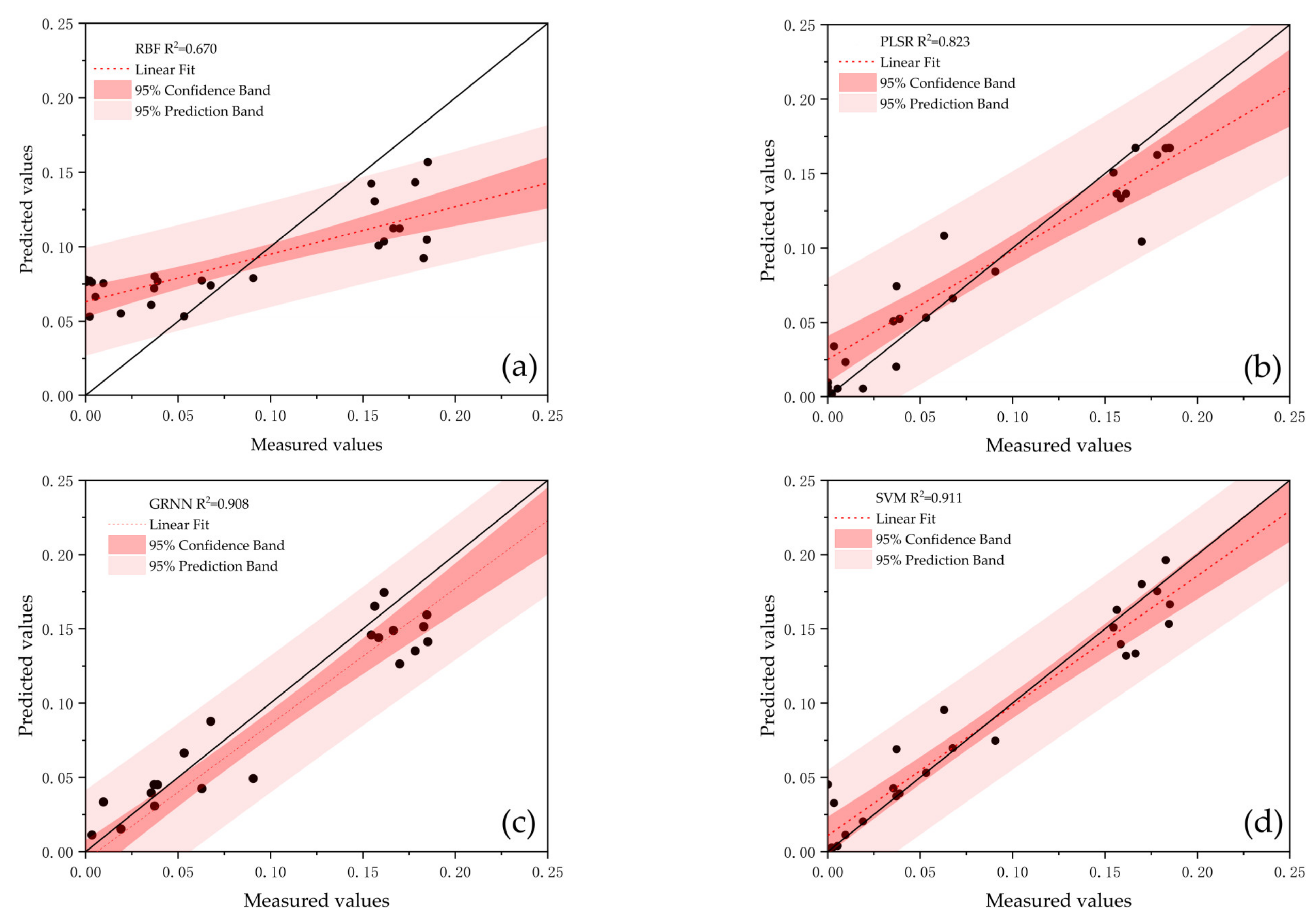
3.1.2. Modeling and Validation of First-Order Derivative Spectra

As shown in Figure 8, both PCA-SVM and PCA-GRNN models have excellent prediction ability, with R² values of 0.942 and 0.899, RMSE values of 0.019 and 0.024. In contrast, the R² of values PCA-RBF and PCA-PLSR are 0.78 and 0.854, with RMSE values of 0.039 and 0.028, respectively. Compared with the parallel polarized spectral data, the prediction model after the first-order derivative has a significantly improved prediction ability.

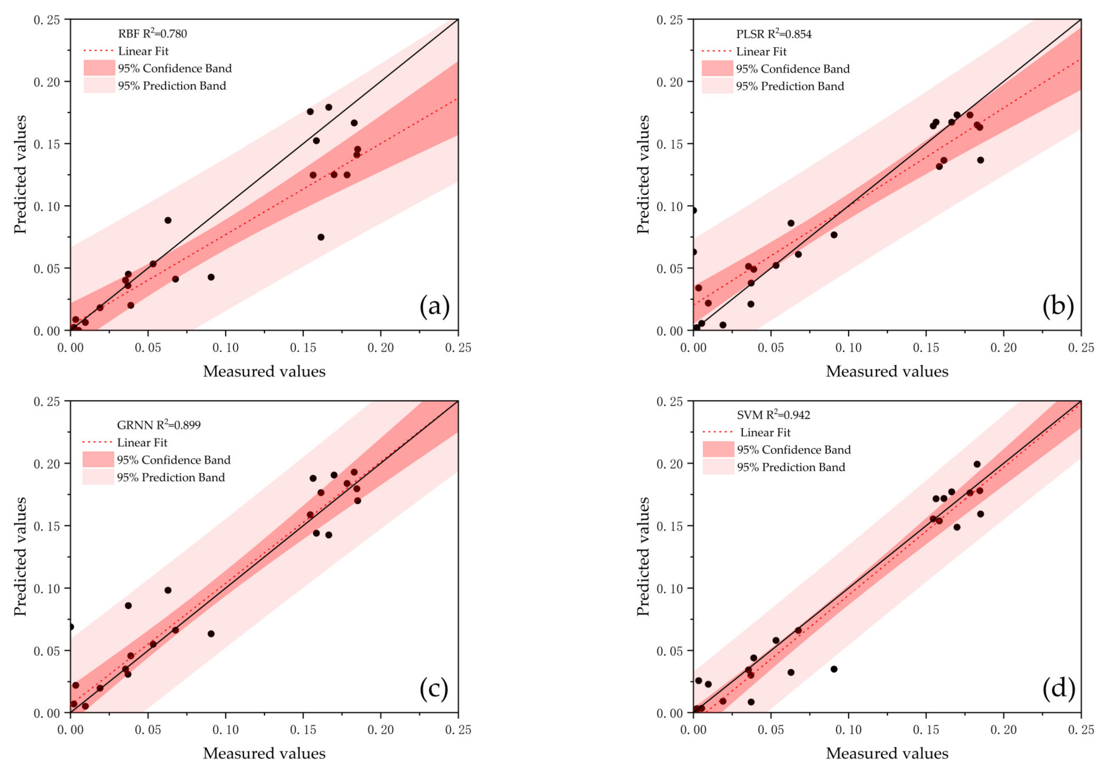
3.1.3. Modeling and Verification of Wavelet Denoising Spectra

For wavelet denoising, the R² values of the four models established by RBF, PLSR, GRNN, and SVM all exceeded 0.85. The PCA-SVM model had the best prediction ability, with an R² of 0.953 and an RMSE of 0.017, indicating that the model had excellent prediction ability. For PCA-GRNN, PCA-PLSR, and PCA-RBF, R² values were 0.948, 0.882, and 0.877, and RMSE values were 0.017, 0.048, and 0.026 (Figure 9), which also have good predictive power, indicating that the model established by the spectral data after wavelet denoising has strong robustness and superior anti-interference ability. The method can not only effectively filter the useless noise and maximize the noise ceiling, but also protect useful data or information from loss to the greatest extent [41].

3.2. Comparative Analysis of the Models

Among the four machine learning models, the PCA-SVM model was the best, and the prediction accuracy was higher than that of the other three models. Specifically, the PCA-SVM model with wavelet denoising transformation had the highest prediction accuracy, with an R² of 0.953 and an RMSE of 0.017. From the perspective of spectral data types, the prediction accuracy of PCA-SVM in the three spectral curve prediction models was relatively stable, all above 0.90, but the PCA-RBF model had low prediction accuracy and was sensitive to data noise. Compared to parallel polarization spectral modeling, the PCA-RBF Model R² based on the first-order derivative spectrum and wavelet denoising spectrum increased by 16.4% and 30.9%, and the PCA-PLSR Model R² increased by 3.8% and 7.2%, respectively. However, the PCA-GRNN model was not sensitive to the noise of the original data due to its high fault tolerance and robustness, and even with preprocessing of the raw data, the predictive power of the model decreased slightly.

As shown in Figure 10, The results of this study indicate that the PCA-SVM model had better prediction accuracy than the PCA-RBF, PCA-PLSR, and PCA-GRNN models for the grade assessment of hydrothermal copper mines at meso-low temperatures, and performed good predictive ability. For the small sample and high-dimensional regression in this study, compared with other machine learning algorithms, the PCA-SVM algorithm did not rely on global data estimation, and could reduce the linear dimension of the original data. It only considered a small number of important support vectors in the input spectrum for decision function regression, effectively avoided the complex process from induction to deduction and multi-dimensional sample space, and significantly reduced the risk of model overfitting and ensured good prediction ability. Compared with the PCA-SVM model, the predicted value of PCA-RBF model had a large underestimation. The center of the hidden layer basis function in the PCA-RBF was selected in the input sample set, which is difficult to reflect the true input-output relationship of the system in many cases, and the RBF still needs to randomly select multiple function centers in the operation, which may produce numerically ill-conditioned problems. Meanwhile, compared with the reflectance spectrum of Yachun Mao et al. [13] and Vahid Khosravi et al. [14] have verified, the visible-near infrared parallel polarized spectrum has a high degree of separation and strong anti-interference ability, which can better eliminate background interference and retain copper content information. However, due to the relatively small number of samples used in the experiment, the PCA-SVM algorithm had certain limitations in the global estimation and nonlinear fitting ability of large-scale training samples when faced with large sample data sets, which needs to be further tested in the actual different mineral intelligent detection and sorting and resource potential assessment [42].

4. Conclusions

This study proposed to employ the visible-near infrared parallel polarized reflectance spectrum detection technology to detect the grade of hydrothermal copper deposits at meso-low temperatures. The PCA-SVM model can have a good predicting precision of copper grade by fusing spectral dimension reduction and a machine learning algorithm. The conclusions are as follows:

The visible-near infrared parallel polarized reflectance spectra have strong polarized reflectance characteristics in the ranges of 600–780 nm and near 1150 nm, and the parallel polarized spectra of different grades have less mixing and crossing, and high separation, which is conducive to the removal and unmixing of spectral redundant information.

Since the initial spectral data have a large dimension and contain some redundant information, the PCA dimension reduction is useful to quickly extract the characteristic variables of parallel polarized hyperspectral data.

The PCA-SVM algorithm has achieved the optimal prediction accuracy in experimental research by using spectral data after wavelet denoising. Compared with PCA-SVM, the PCA-RBF model has a large underestimation. According to the spectral characteristics of different copper samples, different methods to improve the accuracy of the model may be an important research direction of hyperspectral quantitative prediction of copper grade in the future [43,44].

In conclusion, these research results provide the new technical means for the application of hyperspectral measurement technology and for the efficient detection of in situ grades of copper deposits. However, this study is mainly limited to spectral detection in the laboratory, and future studies can be dedicated to predict copper by aerial and satellite imagery.

References

1. Bao, N.S.; Lei, H.M.; Cao, Y.; Liu, S.J.; Gu, X.W.; Zhou, B.; Fu, Y.H. Iron Ore Tailing Composition Estimation Using Fused Visible-Near Infrared and Thermal Infrared Spectra by Outer Product Analysis. Minerals 2022, 12, 382. [Google Scholar] [CrossRef]
2. Fu, Y.H.; Xie, H.F.; Mao, Y.C.; Ren, T.; Xiao, D. Copper Content Inversion of Copper Ore Based on Reflectance Spectra and the VTELM Algorithm. Sensors 2020, 20, 6780. [Google Scholar] [CrossRef] [PubMed]
3. Ambo, A.I.; Iyakwari, S.; Glass, H.J. Selective leaching of copper from near infrared sensor-based preconcentrated copper ores. Physicochem. Probl. Mineral Process. 2020, 56, 204–218. [Google Scholar] [CrossRef]
4. Apua, M.C.; Madiba, M.S. Leaching kinetics and predictive models for elements extraction from copper oxide ore in sulphuric acid. J. Taiwan Inst. Chem. Eng. 2021, 121, 313–320. [Google Scholar] [CrossRef]
5. Noei, S.B.; Sheibani, S.; Rashchi, F.; Mirazimi, S.M.J. Kinetic modeling of copper bioleaching from low-grade ore from the Shahrbabak Copper Complex. Int. J. Miner. Metall. Mater. 2017, 24, 611–620. [Google Scholar] [CrossRef]
6. Starodub, K.; Kuminova, Y.; Dinsdale, A.; Cheverikin, V.; Filichkina, V.; Saynazarov, A.; Khvan, A.; Kondratiev, A. Experimental Investigation and Modeling of Copper Smelting Slags. Metall. Mater. Trans. B Proc. Metall. Mater. Proc. Sci. 2016, 47, 2904–2918. [Google Scholar] [CrossRef]
7. Cai, Y.Y.; Yang, C.H.; Xu, D.G.; Gui, W.H. Quantitative analysis of stibnite content in raw ore by Raman spectroscopy and chemometric tools. J. Raman Spectrosc. 2019, 50, 454–464. [Google Scholar] [CrossRef]
8. Elhamdaoui, I.; Rifai, K.; Iqbal, J.; Mohamed, N.; Selmani, S.; Fernandes, J.; Bouchard, P.; Constantin, M.; Laflamme, M.; Sabsabi, M.; et al. Measuring the concentration of gold in ore samples by laser-induced breakdown spectroscopy and comparison with the gravimetry/atomic absorption techniques. Spectroc. Acta Pt. B Atom. Spectr. 2021, 183, 106256. [Google Scholar] [CrossRef]
9. Van der Meer, F.D.; Van der Werff, H.M.A.; Van Ruitenbeek, F.J.A.; Hecker, C.A.; Bakker, W.H.; Noomen, M.F.; van der Meijde, M.; Carranza, E.J.M.; de Smeth, J.B.; Woldai, T. Multi- and hyperspectral geologic remote sensing: A review. Int. J. Appl. Earth Observ. Geoinf. 2012, 14, 112–128. [Google Scholar] [CrossRef]
10. Tong, Q.X.; Xue, Y.Q.; Zhang, L.F. Progress in Hyperspectral Remote Sensing Science and Technology in China Over the Past Three Decades. IEEE J. Sel. Top. Appl. Earth Observ. Remote Sens. 2014, 7, 70–91. [Google Scholar] [CrossRef]
11. Meyer, J.M.; Kokaly, R.F.; Holley, E. Hyperspectral remote sensing of white mica: A review of imaging and point-based spectrometer studies for mineral resources, with spectrometer design considerations. Remote Sens. Environ. 2022, 275, 13000. [Google Scholar] [CrossRef]
12. Mao, Y.C.; Ding, R.B.; Liu, S.J.; Bao, N.S. Research on Inversion Model of Low-Grade Porphyry Copper Deposit Based on Visible-Near Infrared Spectroscopy. Spectrosc. Spectr. Anal. 2020, 40, 2474–2478. [Google Scholar] [CrossRef]
13. Mao, Y.C.; Huang, J.Q.; Cao, W.; Fu, Y.H.; Zhao, Z.G.; Bao, N.S. Visible-NIR spectral characterization and grade inversion modelling study of the Derni copper deposit. Infrared Phys. Technol. 2021, 115, 103717. [Google Scholar] [CrossRef]
14. Khosravi, V.; Ardejani, F.D.; Aryafar, A.; Yousefi, S.; Karami, S. Prediction of copper content in waste dump of Sarcheshmeh copper mine using visible and near-infrared reflectance spectroscopy. Environ. Earth Sci. 2020, 79, 165. [Google Scholar] [CrossRef]
15. Khosravi, V.; Shirazi, A.; Shirazy, A.; Hezarkhani, A.; Pour, A.B. Hybrid Fuzzy-Analytic Hierarchy Process (AHP) Model for Porphyry Copper Prospecting in Simorgh Area, Eastern Lut Block of Iran. Mining 2021, 2, 1–12. [Google Scholar] [CrossRef]
16. Wang, J.L.; Gao, J.X.; Huang, J.Q.; Qi, Q.H.; Mao, X.Q.; Cao, W.; Ding, R.B.; Mao, Y.C. Quantitative Inversion Modeling Method for Grading Deerni Copper Deposits Based on Visible and Near-Infrared Hyperspectral Data. Can. J. Remote Sens. 2022, 48, 592–608. [Google Scholar] [CrossRef]
17. Sun, L.; Khan, S.; Shabestari, P. Integrated Hyperspectral and Geochemical Study of Sediment-Hosted Disseminated Gold at the Goldstrike District, Utah. Remote Sens. 2019, 11, 1987. [Google Scholar] [CrossRef] [Green Version]
18. Ogen, Y.; Denk, M.; Glaesser, C.; Eichstaedt, H.; Kahnt, R.; Loeser, R.; Suppes, R.; Chimeddorj, M.; Tsedenbaljir, T.; Alyeksandr, U.; et al. Quantification of the Spectral Variability of Ore-Bearing Granodiorite under Supervised and Semisupervised Conditions: An Upscaling Approach. J. Spectrosc. 2021, 2021, 2580827. [Google Scholar] [CrossRef]
19. Shirazy, A.; Ziaii, M.; Hezarkhani, A.; Timkin, T. Geostatistical and Remote Sensing Studies to Identify High Metallogenic Potential Regions in the Kivi Area of Iran. Minerals 2020, 10, 869. [Google Scholar] [CrossRef]
20. Martin, T.; Weller, A.; Behling, L. Desaturation effects of pyrite-sand mixtures on induced polarization signals. Geophys. J. Int. 2022, 228, 275–290. [Google Scholar] [CrossRef]
21. Dubovik, O.; Li, Z.Q.; Mishchenko, M.I.; Tanre, D.; Karol, Y.; Bojkov, B.; Cairns, B.; Diner, D.J.; Espinosa, W.R.; Goloub, P.; et al. Polarimetric remote sensing of atmospheric aerosols: Instruments, methodologies, results, and perspectives. J. Quant. Spectrosc. Radiat. Transf. 2019, 224, 474–511. [Google Scholar] [CrossRef]
22. Xiang, Y.; Yan, L.; Zhao, Y.S.; Gou, Z.Y.; Chen, W. Influence of Surface Roughness on Degree of Polarization of Biotite Plagioclase Gneiss Varying with Viewing Angle. Spectrosc. Spectr. Anal. 2011, 31, 3423–3428. [Google Scholar] [CrossRef]
23. Revil, A.; Vaudelet, P.; Su, Z.Y.; Chen, R.J. Induced Polarization as a Tool to Assess Mineral Deposits: A Review. Minerals 2022, 12, 571. [Google Scholar] [CrossRef]
24. Belyaev, D.A.; Yushkov, K.B.; Anikin, S.P.; Dobrolenskiy, Y.S.; Laskin, A.; Mantsevich, S.N.; Molchanov, V.Y.; Potanin, S.A.; Korablev, O.I. Compact acousto-optic imaging spectro-polarimeter for mineralogical investigations in the near infrared. Opt. Express 2017, 25, 25980–25991. [Google Scholar] [CrossRef] [PubMed]
25. Iglesias, J.C.A.; Gomes, O.D.M.; Paciornik, S. Automatic recognition of hematite grains under polarized reflected light microscopy through image analysis. Miner. Eng. 2011, 24, 1264–1270. [Google Scholar] [CrossRef]
26. Yang, Y.H.; Shi, W.X.; Qiu, J.T. Study on Polarization Spectroscopy of Alteration Minerals. Spectrosc. Spectr. Anal. 2021, 41, 948–953. [Google Scholar] [CrossRef]
27. Ye, S.; Sun, X.X.; Wang, J.J.; Wang, X.Q.; Zhang, W.T. Study on multiangular reflectance polarization characteristics of mineral in visible light waveband. Laser Technol. 2017, 41, 85–90. [Google Scholar] [CrossRef]
28. Svensen, O.; Stamnes, J.J.; Kildemo, M.; Aas, L.M.S.; Erga, S.R.; Frette, O. Mueller matrix measurements of algae with different shape and size distributions. Appl. Opt. 2011, 50, 5149–5157. [Google Scholar] [CrossRef]
29. Liu, J.; Hu, B.; He, X.; Bai, Y.; Tian, L.; Chen, T.; Wang, Y.; Pan, D. Importance of the parallel polarization radiance for estimating inorganic particle concentrations in turbid waters based on radiative transfer simulations. Int. J. Remote Sens. 2020, 41, 4923–4946. [Google Scholar] [CrossRef]
30. Gao, W.; Yang, K.M.; Li, M.Q.; Li, Y.R.; Han, Q.Q. Hyperspectral SFIM-RFR Model on Predicting the Total Iron Contents of Iron Ore Powders. Spectrosc. Spectr. Anal. 2020, 40, 2546–2551. [Google Scholar] [CrossRef]
31. Xu, L.F.; Liu, J.; Wang, C.H. Novel Polarization Conversion Method of Linearly Polarized Light at Specific Incident Angle Based on Plane-Parallel Plate. Optik 2019, 188, 187–192. [Google Scholar] [CrossRef]
32. Wang, P.; Li, N.; Yan, C.H.; Feng, Y.Z.; Ding, Y.; Zhang, T.L.; Li, H. Rapid quantitative analysis of the acidity of iron ore by the laser-induced breakdown spectroscopy (LIBS) technique coupled with variable importance measures-random forests (VIM-RF). Anal. Methods 2019, 11, 3419–3428. [Google Scholar] [CrossRef]
33. Ding, Y.; Zhang, W.; Zhao, X.Q.; Zhang, L.W.; Yan, F. A hybrid random forest method fusing wavelet transform and variable importance for the quantitative analysis of K in potassic salt ore using laser-induced breakdown spectroscopy. J. Anal. At. Spectrom. 2020, 35, 1131–1138. [Google Scholar] [CrossRef]
34. Deng, X.X.; Yang, G.; Zhang, H.; Chen, G.Y. Accurate quantification of alkalinity of sintered ore by random forest model based on PCA and variable importance (PCA-VI-RF). Appl. Opt. 2020, 59, 2042–2049. [Google Scholar] [CrossRef]
35. Li, T.S.; Duan, S.K.; Liu, J.; Wang, L.D. An improved design of RBF neural network control algorithm based on spintronic memristor crossbar array. Neural Comput. Appl. 2018, 30, 1939–1946. [Google Scholar] [CrossRef]
36. Specht, D.F. A general regression neural network. IEEE Trans. Neural Netw. 1991, 2, 568–576. [Google Scholar] [CrossRef] [Green Version]
37. Krishnan, A.; Williams, L.J.; McIntosh, A.R.; Abdi, H. Partial Least Squares (PLS) methods for neuroimaging: A tutorial and review. Neuroimage 2011, 56, 455–475. [Google Scholar] [CrossRef]
38. Ben-Hur, A.; Weston, J. A user’s guide to support vector machines. Methods Mol. Biol. 2010, 609, 223–239. [Google Scholar] [CrossRef] [Green Version]
39. Guenther, N.; Schonlau, M. Support vector machines. Stata J. 2016, 16, 917–937. [Google Scholar] [CrossRef] [Green Version]
40. Zhang, Y.; Wang, D.D.; Li, T. LIBGS: A MATLAB software package for gene selection. Int. J. Data Min. Bioinform. 2010, 4, 348–355. [Google Scholar] [CrossRef]
41. Shim, K.; Yu, J.; Wang, L.; Lee, S.; Koh, S.M.; Lee, B.H. Content Controlled Spectral Indices for Detection of Hydrothermal Alteration Minerals Based on Machine Learning and Lasso-Logistic Regression Analysis. IEEE J. Sel. Top. Appl. Earth Observ. Remote Sens. 2021, 14, 7435–7447. [Google Scholar] [CrossRef]
42. Li, X.H.; Wen, J.; Fu, Y.H.; Mao, Y.C.; Cao, W.; Huang, J.Q.; Zhao, Z.G.; Yu, G. Visible-NIR spectral characteristics and grade inversion model of skarn-type iron ore. Infrared Phys. Technol. 2022, 123, 104170. [Google Scholar] [CrossRef]
43. Desta, F.; Buxton, M.; Jansen, J. Data Fusion for the Prediction of Elemental Concentrations in Polymetallic Sulphide Ore Using Mid-Wave Infrared and Long-Wave Infrared Reflectance Data. Minerals 2020, 10, 235. [Google Scholar] [CrossRef] [Green Version]
44. Shirazi, A.; Hezarkhani, A.; Pour, A.B. Fusion of Lineament Factor (LF) Map Analysis and Multifractal Technique for Massive Sulfide Copper Exploration: The Sahlabad Area, East Iran. Minerals 2022, 12, 549. [Google Scholar] [CrossRef]
Figure 1. (a) Location of the study area in Xiaoyuan village, Yueshan Town, Huaining County, Anhui Province, China. (b) The cores from different construction boreholes in copper deposits. (c) A part of the copper ore samples processed by the crusher and the grinding machine.
Minerals 12 01451 g001
Figure 2. (a) SVC HR-1024; (b) parallel polarized reflection spectrum measurement system.
Minerals 12 01451 g002
Figure 3. Parallel polarized reflection spectra.
Minerals 12 01451 g003
Figure 4. (a) First-order derivative spectra of parallel polarization reflection; (b) polarization reflection spectra processed by wavelet denoising.
Minerals 12 01451 g004
Figure 5. (a) PCA of the parallel polarization spectrum, (b) PCA of first-order derivative spectrum and (c) PCA of wavelet denoising spectrum.
Minerals 12 01451 g005
Figure 6. The flow chart of copper grade prediction.
Minerals 12 01451 g006
Figure 7. Model prediction of parallel polarization spectral data (a) RBF, (b) PLSR, (c) GRNN, (d) SVM. The measured values and predicted values are expressed as the copper grade of the test samples and the predicted value of the model. The black line shows the 1:1 relationship and the dashed line shows the model trend. In the data augmentation domain, the input spectra with ranges of 450–1700 nm for Copper grade were selected to develop multivariate regression models. The SVM model falls within the largest number of points within the 95% confidence band.
Minerals 12 01451 g007
Figure 8. Model prediction of first-order derivative spectral data (a) RBF, (b) PLSR, (c) GRNN, (d) SVM. The measured values and predicted values are expressed as the copper grade of the test samples and the predicted value of the model. The black line shows the 1:1 relationship and the dashed line shows the model trend. In the data augmentation domain, the input spectra with ranges of 450–1700 nm for copper grade were selected to develop multivariate regression models. The SVM model falls within the largest number of points within the 95% confidence band.
Minerals 12 01451 g008
Figure 9. Model prediction of wavelet denoising spectral data (a) RBF, (b) PLSR, (c) GRNN, (d) SVM. The measured values and predicted values are expressed as the copper grade of the test samples and the predicted value of the model. The dashed line shows the 1:1 relationship and the black line shows the model trend. The black line shows the 1:1 relationship and the dashed line shows the model trend. In the data augmentation domain, the input spectra with ranges of 450–1700 nm for copper grade were selected to develop multivariate regression models. The SVM model falls within the largest number of points within the 95% confidence band.
Minerals 12 01451 g009
Figure 10. Comparative analysis of R2 and RMSE of three spectral data models.
Minerals 12 01451 g010