A Comparative Study of Porphyry-Type Copper Deposit Mineralogies by Portable X-ray Fluorescence and Optical Petrography


Department of Environmental, Geographical, and Geological Sciences, Bloomsburg University of Pennsylvania, Bloomsburg, PA 17815, USA
*
Author to whom correspondence should be addressed.
Minerals 2020, 10(5), 431; https://doi.org/10.3390/min10050431
Submission received: 30 March 2020
/
Revised: 6 May 2020
/
Accepted: 8 May 2020
/
Published: 11 May 2020
(This article belongs to the Special Issue Innovative and Applied Research on Platinum-Group and Rare Earth Elements: Dedicated to the Work and Memory of Dr. Demetrios G. Eliopoulos, IGME (Greece))
Abstract
:Porphyry-type deposits are crucial reserves of Cu and Mo. They are associated with large haloes of hydrothermal alteration that host particular mineral assemblages. Portable X-ray fluorescence analysis (pXRF) is an increasingly common tool used by mineral prospectors to make judgments in the field during mapping or core logging. A total of 31 samples from 13 porphyry copper deposits of the Western Cordillera were examined. Whole-rock composition was estimated over three points of analysis by pXRF. This approach attempts to capture the rapid and sometimes haphazard application of pXRF in mineral exploration. Modes determined by optical petrography were converted into bulk rock compositions and compared with those determined by pXRF. The elements S, Si, Ca, and K all were underestimated by optical mineralogy, and the elements Cu, Mo, Al, Fe, Mg, and Ti were overestimated by optical mineralogy when compared with pXRF results. Most of these porphyry samples occur in veined porphyritic quartz monzonite that is characteristic of these deposits. Sulfide and silicate vein stockworks are pervasive in most of the samples as well as dissemination of sulfides outwards from veinlets. Ore minerals present include chalcopyrite and molybdenite with lesser bornite. Chalcocite, digenite, and covellite are secondary. Potential sources of analytical bias are discussed.
1. Introduction
1.1. Porphyry-Type Deposits
Porphyry-type deposits, often termed just “porphyry deposits”, represent one of the most studied geological systems on Earth, and the economic fortunes that entail from the proper extraction of the metals found in these deposits have pushed the academic and industrial communities to study them. This deposit model that came to popularity in the mid-late 1960s [1,2], was summarized by Sillitoe [3] and then later expanded upon [4,5,6,7,8]. Porphyry-type deposits represent 60% of world Cu production annually, and 65% of known world Cu resources [6]. These deposits also represent half of the world’s Mo production and may also contain economic grades of Ag, Zn, W, Sn, Re, and Au [7]. Low-grade resources of Pt-group elements are also possible [9,10]. Tonnages commonly exceed one billion [8]. An example of a deposit of this scale is Bingham Canyon (Utah), a deposit analyzed in this study, at 2.6 Gt of ore [11]. These high tonnages are offset by lower grades of metals extracted, typically between 0.5–1.0 wt% Cu [7]. The deposits are typically found along convergent plate margins where the subduction of an oceanic plate below the adjacent continental or oceanic plate drives partial melting, thus creating arc magmatism [3]. Although similar types of deposits occur in rarer continental-continental orogens [12]. These magmatic arc systems allow metals found in greater concentrations deeper in the earth to rise buoyantly as magma and emplace themselves as intrusive bodies capable of metal concentration. These systems cool, and depressurization processes occur such that metals are highly concentrated in an immiscible hydrothermal fluid located at the top of such intrusive bodies. These metals are then injected into the surrounding rock by hydraulic fracturing forming large stockworks of cross-cutting veins that contain concentrated metals [8]. The particular samples analyzed in this study are from the Western Cordillera of the Americas. Deposits of this type are essential to the growth of economies in developing countries, such as Chile where copper mining has contributed an average of 10% of GDP over the past 20 years [13]. Deposits found along the Western Cordillera of North America are, or have been influential regarding the economies of the regions and countries these deposits are found in.
1.2. Portable X-ray Fluorescence
X-ray fluorescence analysis produces compositional data by exciting the sample in question with X-rays. Those X-rays will ionize the sample’s atoms by knocking out core-shell electrons. Outer-shell electrons will then fall/relax into the subsequent core-shell vacancy. As this involves a loss of energy, a photon is emitted with energy equal to the difference in electron orbitals. The energy quantum of the photon is unique to the element in question and is also in the X-ray portion of the electromagnetic spectrum. Thus, the X-ray’s energy is characteristic of the element and the number of photons with that quantum is proportional to the element’s concentration in the sample. Engineering advances over the last few decades have allowed this laboratory-scale instrumentation to be miniaturized into a portable format. A variety of commercial portable and handheld X-ray fluorescence analyzers are now available [14]. Portable X-ray fluorescence (pXRF) is an increasingly common method for on-site and rapid materials analysis. For exploration and development of mineral deposits, it has particularly been applied to geochemical exploration [15,16,17], assessments of soil contamination [18], core logging [19], and mineralization type [20,21]. This is a method that requires little training, is portable, fast, fairly affordable, and can provide useful data. However, compared to other lab methods (including more sophisticated, lab-based, and non-portable XRF analyzers), analyses can be very susceptible to measurement bias, insensitivity to elements lighter than Mg or Al, and matrix effects [22,23]. Whereas “portable” can refer to a variety of XRF configurations, for this study it refers to handheld instruments, typically resembling a pistol.
As pXRF is often used as a tool by field or core logging geologists, it is typically one of the first analytical methods applied to samples. The absence of typical sample preparation in the field, the small sample point size, and human bias in selecting what points to analyze introduce additional uncertainties to the data. Although they may be collected under less than optimal analytical conditions, results from pXRF can influence decisions regarding geologic mapping, cross-sections, and selection of samples for more detailed assay/investigation. Another investigative method that can follow pXRF is optical petrography. In fact, data from pXRF may influence a geologist to select a sample for thin sectioning and petrographic examination. A geologist can later re-interpret and reconcile the pXRF data in the context of sample mineralogy. Likewise, pXRF data can be useful in interpreting the observed mineralogy in thin sections. The combined use of complementary but independent methods such as pXRF and optical petrography has the potential to augment the abilities of the investigating geologist in a fairly fast and economical manner.
In addition to its portability and ease of use, pXRF is typically non-destructive. Outcrop, drill core, grab samples, soil, and thin section billets (this study) can be analyzed with no crushing, grinding, fusion, dissolution, etc., that lab-based XRF or ICP-MS require. Similarly, polished thin sections that can be made from a modest amount of sample, are not expended when examined, preserve mineral textures, and can later be analyzed by other methods such as electron microscopy or other microbeam methods.
We present that pXRF used in a rapid fashion with no standardization, in the manner of many field applications, can still provide semi-quantitative data that are useful to answer geological questions in the field. We simulate these haphazard conditions using point analysis on thin-section billets of rock samples from porphyry-type deposits. Sources of analytical uncertainty arising from these conditions are examined and discussed. The results are compared with those of optical petrography, another common, albeit much older, standby in non-destructive geological sample characterization.
2. Materials and Methods
2.1. Sample Locations
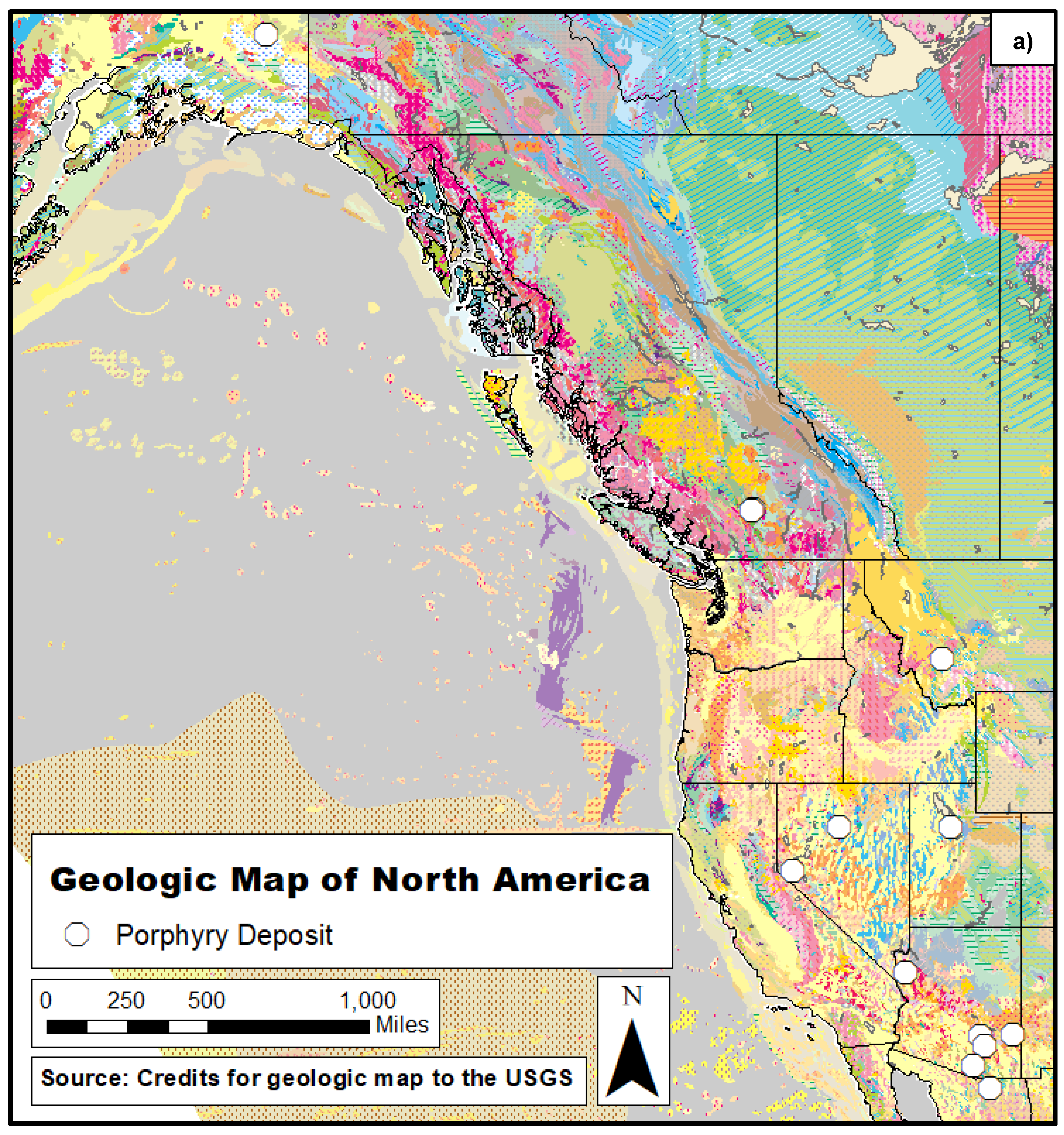
The 31 hand samples used in this comparative study are from 13 different deposits found along the oceanic-continental subduction zone of the Western Cordillera of North America (Table 1, Figure 1). These are Cu ± Mo porphyry-type deposits and represent different portions within each deposit (for those deposits with more than one sample). The samples include specimens from the hypogene and supergene zones of these deposits. The zone of interest for this study was primarily the hypogene. These samples were collected and donated by Peter H. Kirwin and John R. Ray, formerly of the American Copper and Nickel Company.
2.2. Analytical Methods
In this comparative study two methods were used to determine the overall mineralogy of the samples. These methods include using pXRF giving elemental weight percent readings for each sample, as well as using polarized transmitted and reflected light microscopy to estimate mineral abundances and related textures. Limiting the study to these two methods allows the investigation to be conducted in an essentially non-destructive manner at minimal cost.
2.2.1. Optical Petrography
The 31 samples were selected from a larger collection on the basis of interesting mineralogy or textures visible in hand samples, geographic location, and budget limitations (for thin sectioning). They were cut into rectangular billets by a rock saw (e.g., Figure 2). The billets were then used to shave off 30 µm × 26 mm × 46 mm polished thin sections for further analysis under a petrographic microscope. The thin sectioned samples were then examined under a Leica DM2700 P microscope (Leica Microsystems Inc., Buffalo Grove, IL, USA) in transmitted and reflected light modes. In the first assessment of these thin sections, the textures were documented along with a qualitative listing of minerals present in each sample. More in-depth qualitative observations were then made at this point, and the genetic sequencings of minerals along with their characteristics were noted. In the second extensive assessment of these samples using petrographic methods, the overall mineral modes were determined. This assumed that the mineral abundances in terms of thin section area are representative of the volume% abundances (true modes) of the mineral.
2.2.2. Portable X-ray Fluorescence
When the overall modes were determined for each sample, the bulk elemental compositions were then determined by pXRF analysis of the flat face of the corresponding billet the thin section was cut from. A Thermo Scientific NitonTM XL3t-950 GOLDD+ (Thermo Fisher Scientific, Waltham, MA, USA) was the pXRF analyzer used in this study. All analyses were done in Mining Cu/Zn mode. A 10-minute warmup and system check were conducted prior to every session of analyses. Analysis quality was checked for instrument drift using two manufacturer-provided standards: CRM 180-649 NIST 2709a and blank 180-647 99.995% SiO2 blank that were checked using the pXRF prior to the study and after the study. These standards are supplied as fine homogenized powders. No significant deviation from known values (>10%) was noted. Samples were analyzed with pXRF for a 120-s interval, with 30 s each for the main (Mo, Zr, U, Rb, Th, Pb, Se, As, Hg, Nb, Cu, Ni, Co, Fe, Mn, Sr, Y), low (Sc, Ca, K, V, Ti, Cr), high (Ba, Cs, W, Te, Sb, Sn, Cd, Ag, Pd, La, Ce, Pr, Nd), and light (Al, P, Si, Cl, S, Mg) characteristic X-ray ranges of elements using a series of filters. This allowed for fairly precise readings of elemental weight percent (wt%) for each sample. Each sample was analyzed three times in three separate locations on the sectioned surface of the billet in an attempt to address inhomogeneities within these billets. The average elemental composition was determined using all three readings per sample. In the case of three very different analyses, a fourth location was analyzed on the billet.
2.3. Data Calculation
Modes from petrographic microscopy observations were converted into estimates of bulk elemental composition for each sample. The modes, taken as volumetric percentages, were converted into mineral mass percentages using established densities. These mineral mass proportions were then converted into elemental proportions. Density and compositional values were sourced from webmineral.com. Elements not analyzable by pXRF (mostly elements lighter than Mg) were left out of calculations in the modal abundance conversion to allow for simpler comparison. Estimates of solid solution members were made for plagioclase, chlorite, and muscovite. In terms of atoms per formula unit (apfu) it is assumed that plagioclase has 0.5 Na, 0.5 Ca, 1 Al, and 3 Si, chlorite has 3.75 Mg and 1.25 Fe, and biotite has 2.5 Mg and 0.5 Fe.
The whole-rock compositions calculated from the modes were then compared with the average whole-rock compositions determined by pXRF for purposes of comparison and to audit the accuracy of each method against the other.
3. Results
3.1. Hand Sample Examination
At the hand sample scale, prior to the thin sectioning of each sample, porphyry-type copper deposit characteristics were evident (e.g., Figure 2; see [24] for a review). Characteristic veining associated with hydraulic fracturing was seen in many samples as mineral assemblages of silicates and sulfides with rare carbonates. Sulfides associated with the hypogene system are typically dominated by chalcopyrite and pyrite. Silicates in this zone displayed less alteration than that of more near-surface samples, maintaining the dominantly quartz monzonitic mineralogy seen in a majority of hypogene samples although chalky sericitization of feldspars is common in the host rocks. In hand samples, characteristic zoning of alteration could be seen with some ambiguity but overall a grade from hypogene to supergene alteration was clear (c.f., [7]). The oxidation and hydration of hypogene sulfide minerals was a clear indicator of supergene alteration.
3.2. Optical Petrography
In thin sections, the observations made of the hand samples were expressed in clearer detail, and the overall modes observed in hand samples are consistent with those observed at a microscopic level (Table 2, Figure 3). The main sulfides present in hypogene samples show characteristic veins/veinlets of chalcopyrite, bornite, and/or pyrite (e.g., Figure 3g,f), along with sulfide grains disseminated distally from veinlets (e.g., Figure 3a,h). These veinlets also comprise hydrothermal quartz along with sericite and chlorite, and rarely calcite (e.g., Figure 3g). Molybdenite was the only Mo-bearing sulfide seen in thin section (e.g., Figure 3b,c,h, Table 2). Samples affected by some supergene fluid alteration have distinct mineralogies. The sulfide assemblages of the hypogene zone, though starting rich in Cu sulfides, quickly grade into zones of pyrite showing a lack of Cu concentration distally (e.g., Figure 3f). In the supergene samples, chalcocite, covellite, and/or digenite are observed as rims on partially replaced pyrite and/or chalcopyrite (Figure 3a). Specular hematite (possibly with magnetite in some cases) occurs in some samples and also appears to be hydrothermal. This is distinct from the late hematite after sulfides seen in some partially oxidized samples (see below).
The host rocks vary depending on the particular deposit. Most are porphyritic hypabyssal/intrusive rocks that are quartz monzonitic/latitic, although granitic/rhyolitic and granodioritic/dacitic assemblages occur (c.f., [26]). Primary quartz is present in varying amounts but silicification is prevalent. Biotite, apatite, rare amphibole, and rare zircon are also present as primary minerals. In addition to silicification, potassic alteration, sericitization (mostly muscovite after plagioclase and orthoclase) and chloritization (of biotite) are prevalent (e.g., Figure 3e). Carbonation (of plagioclase and mafic minerals) occurs but is rare. In many samples, silicification and/or sericitization obliterated much of the primary phases and textures.
Supergene oxidation is evident in some samples by partial replacement of pyrite by masses of hematite ± goethite. These samples also showed some spots of decomposition of Cu-bearing sulfides as a greenish tinge or patina (i.e., chrysocolla-malachite) on hand samples, however, none of the areas thin sectioned contained these spots to any significance.
3.3. Estimation of Bulk Compositions from Modes
The estimated bulk rock compositions for these modes was calculated by converting the observed mineral abundances to weight proportions, and then elemental proportions based on idealized compositions of the minerals. Based on the observed minerals, only the elements Mg, Al, Si, P, S, K, Ca, Ti, Fe, Cu, and Mo were considered (Table 3).
3.4. Portable X-ray Fluorescence Analysis of Bulk Compositions
Analysis by pXRF provided compositional information in terms of elements Mg and heavier (Table 4). Overall composition across the samples varies significantly. Significant variations in Mg, Si, P, S, K, Ca, Ti, Fe, Cu, and Mo content occur. Other elements analyzed for, but are low in concentration (<0.5 wt%) and do not show significant variation are: Cl, V, Cr, Mn, Co, Ni, Zn, As, Se, Rb, Sr, Y, Zr, Nb, Ag, Cd, Sn, Sb, Ba, La, Ce, Pr, Nd, W, Au, Pb, Th, and U. Concentrations for V, Co, Se, Y, Sn, Sb, Au, and U were essentially non-detectable (less than approximately 0.001 wt%). Uncertainty in analyses is dominated by the variance between spots compared to the actual instrumental error with the possible exception of Mg, the element with the highest uncertainty in terms of measurement.
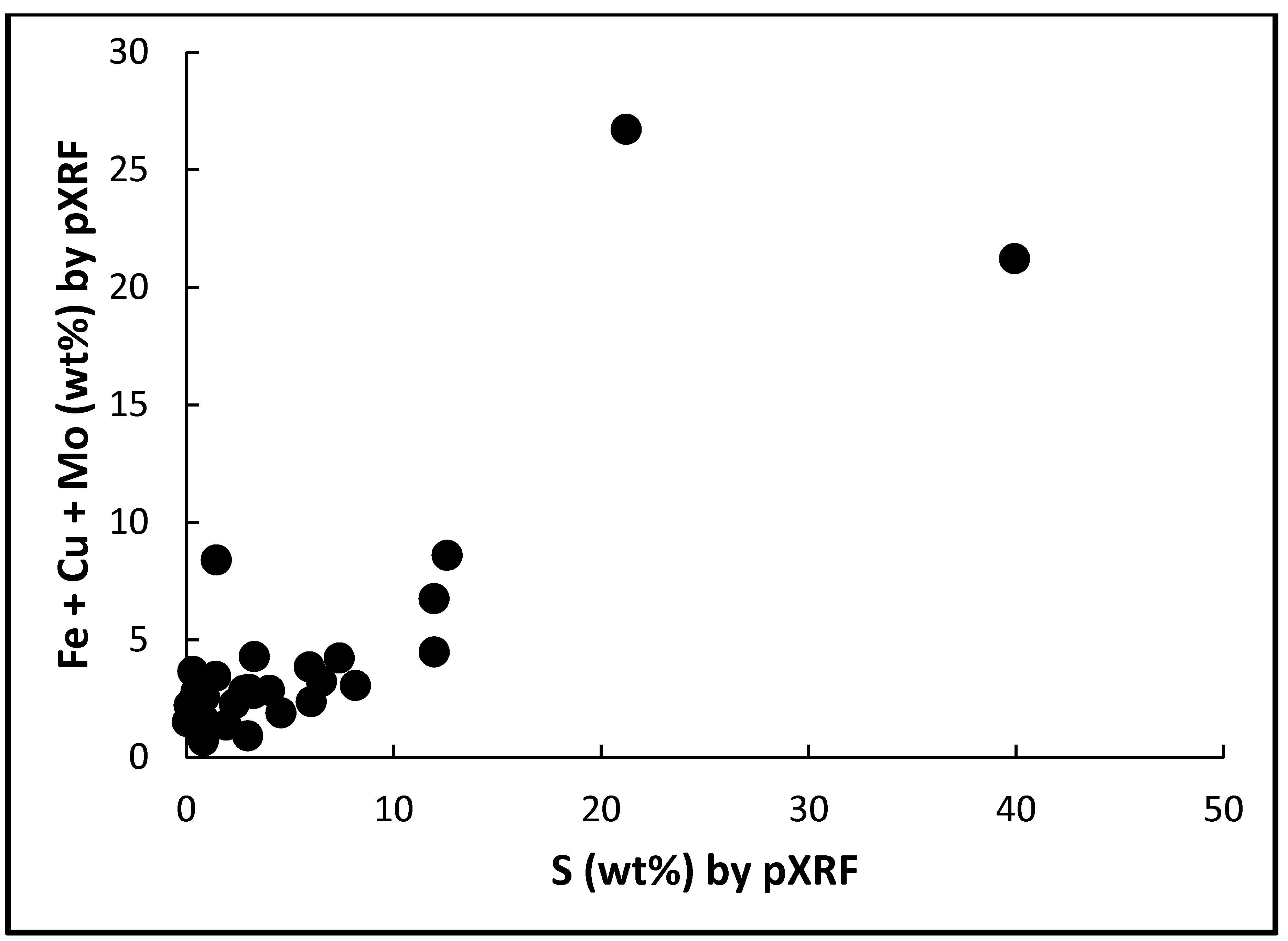
In terms of the economic metals, Cu grades vary from 0 to 14.8 wt% (mean: 0.8 wt%) and Mo grades vary from 0 to 0.3 wt% (mean 0.02 wt%). For the other elements, silicon is the most abundant and ranges from 23.2 to 53.8 wt% (mean: 37.4 wt%). Al is the second most consistently abundant element (0.1 to 8 wt%, mean: 4.9 wt%) followed by K (0 to 8.5 wt%, mean: 3.5 wt%). Elements that are high abundance in some samples (those with high sulfide mineral content) are Fe (0.5 to 20.8 wt%, mean: 3.6 wt%) and S (0.1 to 40 wt%, mean: 5.4 wt%). Less significant variations are Mg (0 to 3.5 wt%, mean: 0.6 wt%), P (0 to 0.4 wt%, mean 0.1 wt%), Ca (0 to 3.2 wt%, mean 0.8 wt%), and Ti (0 to 1.2 wt%, mean 0.3 wt%). The sum of chalcophile element concentrations: Fe, Cu, and Mo, correlate with S content (Figure 4).
3.5. Comparison of Bulk Compositions from Both Methods
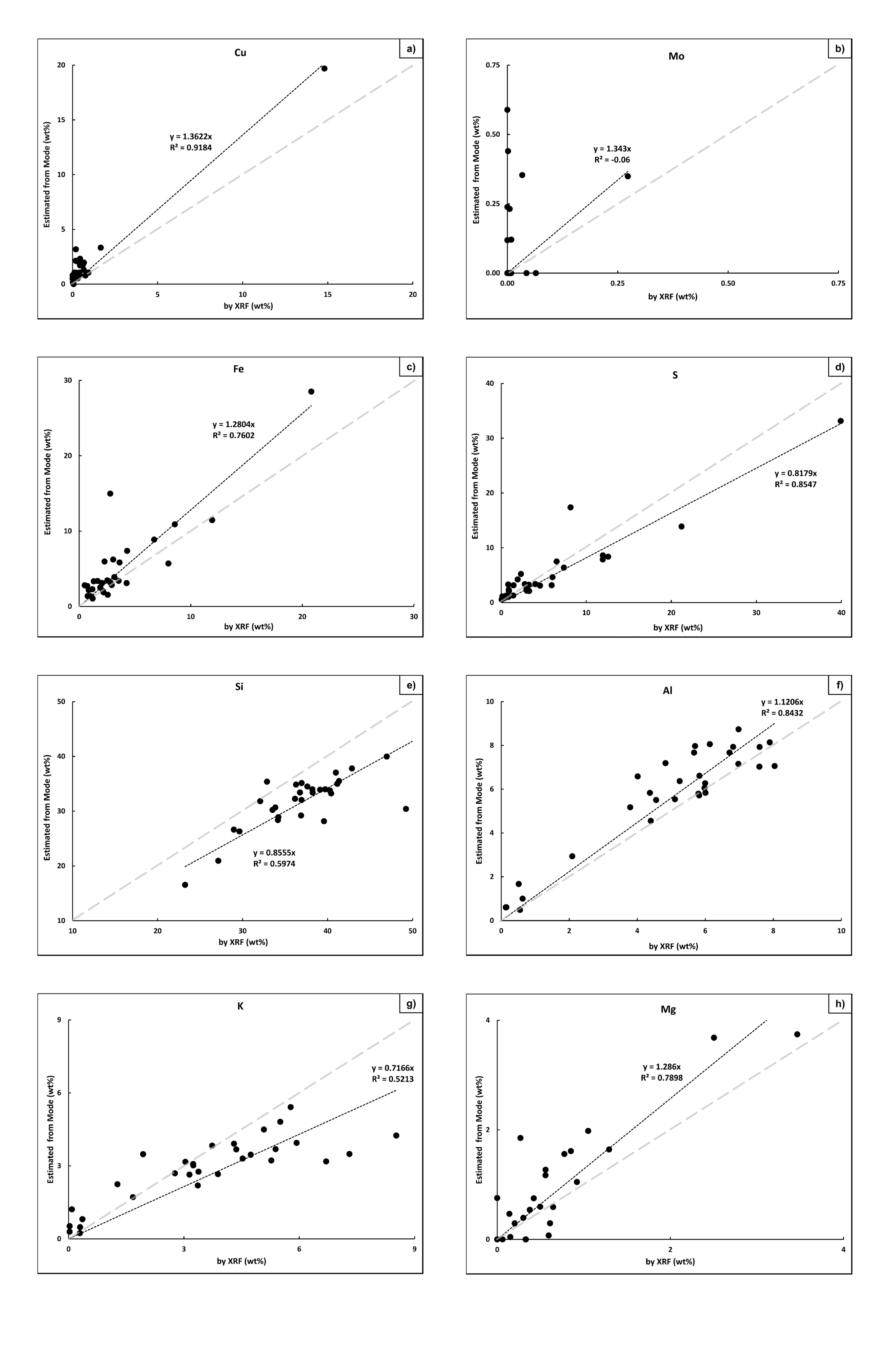
Calculated bulk rock composition (in terms of selected elements) based on estimated modes from optical petrography and the estimated bulk rock compositions based on pXRF analyses are compared on an element-by-element basis (Figure 5).
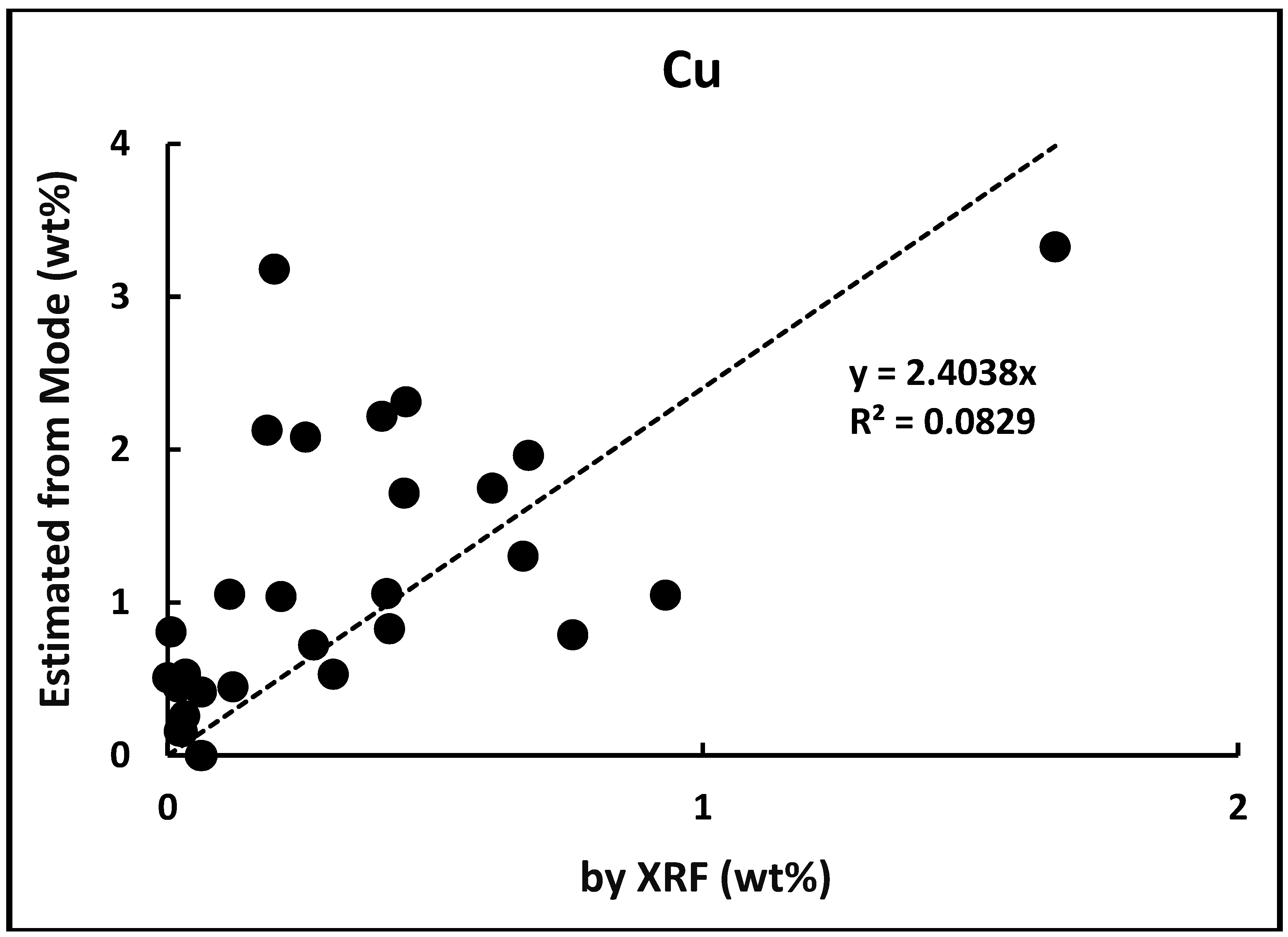
The degree of correlation between the two methods depends on the particular element. The lightest and the heaviest elements are systematically overestimated by optical petrography compared to pXRF: Cu, Mo, Fe, Al, Mg, and Ti (Figure 5a–c,f,h). In contrast, the mid-atomic number elements are underestimated by optical petrography compared to pXRF: S, Si, K, Ca, and P (Figure 5d,e,g). The element that shows the closest 1:1 correlation between the two methods is Al (Figure 5f), followed by Si (Figure 5e). The poorest correlations are shown for Cu and Mo (Figure 5a,b). The correlation for Cu is far worse when the single high-Cu sample (IP-12) is omitted from the fit (Figure 6). The best trendline fits are for Cu, S, and Al (Figure 5a,d,f). However, the fit is very poor in terms of Cu if sample IP-12 is omitted (Figure 6). The worst fit is shown by Mo (R2 = −0.06, Figure 5b), followed by Ca (R2 = 0.443), Ti (R2 = 0.4662), and P (R2 = 0.4721). The balances (remaining wt% not attributed to a single element) are slightly overestimated by mode compared to pXRF by a factor of 1.0623, and with an adequate fit (R2 = 0.7361). Significant outliers from these trends are Bu-06: higher Fe and S, but lower Si by mode than by pXRF, Bi-02: lower K by mode than by pXRF, F-02, higher K by mode than by pXRF, L-01: higher Cu by mode than by pXRF, and Mo-02: higher Mg by mode than by pXRF.
4. Discussion
There are multiple factors affecting each method that may bias results. These affect the accuracy and precision of the mode-based or pXRF-based methods, and the correlation of the two.
4.1. Causes of Poor Correlation
In terms of optical petrography, melanocratic (i.e., mafic minerals, sulfides, and oxides) minerals are typically overestimated compared to leucocratic minerals (i.e., felsic minerals, carbonates, and phosphates; c.f., [27]). Sulfide minerals are exclusive hosts for Cu and Mo in the samples. Similarly, biotite-chlorite and rutile are the major hosts for Mg and Ti, respectively. Biotite, chlorite, hematite, and sulfides are also the hosts for Fe. These minerals are all dark-colored or opaque in TPPL and readily noted. Colorless or light-colored minerals in TPPL such as quartz, muscovite (as sericite), orthoclase, plagioclase, calcite, and apatite collectively host the bulk of Si, K, Ca, and P. The residency of Al is less clear as it is overestimated by optical petrography (Figure 5f) and is an important constituent (along with K and Si) of biotite-chlorite but is a more significant component of the feldpars and sericite. Human error as systematic visual overestimation of biotite and chlorite during optical petrography would give a positive bias to the Mg, Fe, and Al calculated by mode; particularly if it was at the expense of quartz content. The other element with unusual behavior is S in that it is underestimated by optical petrography. As the only S-bearing phases noted are sulfides, it would be expected that optical mineralogy would overestimate this element as with Fe, Cu, and Mo. These elements track with S (Figure 4), but it is possible another S-bearing phase was overlooked, such as barite, anhydrite, or gypsum. Barite is not likely as a negligible Ba content was noted by pXRF in all samples. Hypogene anhydrite occurs in porphyry-type deposits (e.g., [28]), and can be fairly common [5,29]. Another cause for S underestimation from the mode is misidentifying sulfide minerals that are S-rich (chalcopyrite and covellite) for S-poor phases (bornite, digenite, and chalcocite). However, the most abundant S-bearing mineral is pyrite, and a similar underestimation is not present with Fe; nor are those two groups of Cu-sulfides easily confused in RPPL. It may be that the pXRF systematically overestimates S content of the samples and further calibration should have been applied. Systematic overestimation of S (along with P, Cu, and Mg) by pXRF has been observed with field analysis of soils [30]. However, Roman Alday et al. [16] found that for samples from the Elatsite porphyry-type deposit, pXRF overestimates Fe and K, and underestimates Mg compared to more intensive laboratory methods. Matrix effects on pXRF vary with mineral assemblages and development of calibration standards is reliant on rock type [23,31]. The poorest correlation of the chalcophile elements is for Mo. Economic grades in porphyry-type deposits range from approximately 0.1 to 0.3 wt% Mo, although lower grades in the presence of another commodity such as Cu are common [32]. This is a lower grade than Cu due to the higher valuation of Mo, typically 2× to 3× the per-pound metal price. This grade range approaches the limit of detection for Mo by most pXRF units in a typical silicate–sulfide matrix. The result is that although molybdenite is fairly distinct and easy to identify in reflected light, it may be in trace concentrations that contribute grades too low to be detected by pXRF. Thus, mode-based estimates of grade will likely be higher than those detected by pXRF. The selection of the pXRF analytical spots may also play a role (see Section 4.4).
4.2. Outliers from Trends
Five samples, in particular, plotted as major outliers from the trends established by the rest of the data for one or more elements. These are most likely the result of errors in visual estimation of modes as discussed above. Bu-06 has 2.8 wt% Fe by pXRF and 15 wt% Fe by mode. This is accompanied by a similar overestimation of S by mode and underestimation of Si by mode. This is most likely due to the overestimation of pyrite at the expense of quartz. Bi-02 has 8.5 wt% K by pXRF and 4.2 wt% K by mode. This is likely from an underestimation of muscovite (as sericite). F-02 has 1.9 wt% K by pXRF and 3.5 wt% by mode. The overestimation of potassic phases is likely. Orthoclase is most probable as it has a higher proportion of K to Al than muscovite and there is not a significant Al outlier for this sample. There is no accompanying Fe and/or Mg outlier, so biotite-chlorite is not likely. L-01 has 0.2 wt% Cu by pXRF and 3.2 wt% Cu by mode. This is most likely due to an overestimate of the modal abundance of chalcopyrite. Mo-02 has 0.3 wt% Mg by pXRF and 1.9 wt% Mg by mode, most likely due to an overestimation of a mafic mineral, such as chlorite. It should be noted, that the element with the highest instrumental error is Mg (Table 4).
4.3. Assumptions of Mineral Composition
Other than errors in visually estimating the mode of a sample or in misidentifying phases, another source of error in calculating the bulk rock composition from the mode is the assumed composition of the mineral phases. Chlorite, biotite, and plagioclase all have assumed compositions in terms of solid solution components for the purposes of translating the modes into compositional data. These assumptions are not supported by any mineral analysis such as electron microprobe analysis. Minerals such as biotite can vary in composition between different deposits and within single deposits. Magmatic biotite of the host is typically more Fe-rich than the later hydrothermal biotite [6], largely depending on what alteration zone (i.e., potassic vs. phyllic) they are from (e.g., [33]). There was no distinction between these parageneses of the same minerals during the determination of the modes. As chlorite is largely a product of biotite alteration in these deposits, a similar degree of compositional variation is expected. Likewise, plagioclase in porphyry deposits varies in composition. For example, plagioclase from Sierrita ranges from Ab25 to Ab45 [34]. The simplified estimation of a molar 1:1 ratio of Na:Ca in plagioclase in this study is likely why bulk compositions based on modes overestimates Ca content. Muscovite and chlorite from the Highland Valley district (that includes the Lornex and Bethlehem deposits) range in composition 2.2–2.6 Al apfu and 0.5–3.5 Mg apfu, respectively [35].
4.4. Sampling Biases
A further source of disparity between the results of the two methods lies in sampling. Though the thin section is cut from the billet, there may be fairly distinct differences in mode between a 0.03 mm thick section and a ~10 mm thick billet. The thin section is essentially a 2D representation of a 3D rock, whereas the pXRF analysis is an average of three different spots on the billet, each 8 mm in diameter (the default aperture size on the Niton XL3t), with an effective sampling depth (d) expressed by Equation (1):
where d is the sampling depth from which 99% of the signal is sourced, m is the mass per unit area sampled and ρ is sample density [23]. For the samples, the least dense abundant mineral is plagioclase (ρalbite = 2.61 g/cm3) and the densest is pyrite (ρpyrite = 5.01 g/cm3). Denser samples (i.e., sulfide-rich) will approach more surficial analyses, whereas sampling depth will be deeper for samples dominated by felsic minerals. If the billet has compositional variations in the vertical (depth) sense, then the spot analyses become pseudo-bulk analyses of a cylinder 8 mm in diameter a a depth that is a function of sample density. Similarly, in the horizontal sense, three spots at 50.27 mm2 totals ~150.8 mm2, whereas the thin section is up to 1196 mm2 in total area. Accounting for 3 mm margins around the billet, this reduces to 800 mm2 of sample area. Thus, this method in the best case, sampled only ~19% of the sample area and assumes it is representative of the other 21%. Sampling precision for finer-grained rocks by pXRF has been shown to be ≤5% relative standard deviation, but much higher for coarser-grained samples [36]. The thin section is a ~60 µm slice off of the top of the billet that is subsequently ground down to 30 µm. Sample heterogeneity is typically on a scale an order of magnitude larger. Differences in thin section and sample billet surface are negligible in comparison to the other discussed sources of uncertainty. Although most of the rocks in this sample suite are hypabyssal to volcanic, the presence of phenocrysts and veins/veinlets increases the number of measurements required to achieve the same precision that would be possible compared to an un-veined, aphyric sample. The large sample standard deviations across the spot analyses ((s)spot) for many samples illustrates this (Table 4). Samples with a high degree of heterogeneity in terms of multiple elements are all the Ithaca Peak samples, Be-4, Bu-2, Bu-7, F-3. Mo-6, OH-1, and S-4.
d = m/ρ
4.5. Applicability of pXRF to Mineral Exploration
Compared to the classic standard of optical petrography, pXRF is faster, more accessible, portable, and more easily conducted with little training. It is not a replacement for laboratory methods as it cannot reliably reach the levels of precision and accuracy required to meet standards for mineral resource reporting in terms of NI 43-101 (National Instrument 43-101 is the Canadian code for the Standards of Disclosure for Mineral Projects. It sets standards for reporting mineral resource information such as grade, tonnage, etc., and what methods are suitable for measuring them to an adequate degree of certainty) or JORC (Joint Ore Reserves Committee Code is essentially the Australian equivalent to NI 43-101) guidelines, but with calibration, it can achieve a low but useful level of quantitative certainty (e.g., [16,20,21]). However, for quick decisions regarding unknown samples in the field or core shed, semi-quantitative analysis is satisfactory in order to make rough interpretations on whether to collect a sample for more detailed assay/examination. Similarly, pXRF can be used to guide petrographic examinations in terms of possible (and impossible) phases present as with this study.
Although this study attempts to simulate “field” use of pXRF, the analytical conditions for this study were more optimal and controlled than those typical of field or even core shed settings. Analyzed surfaces of the billets were fresh, clean, and flat. Samples from outcrop, float, or trenches may have soil, lichen, or other debris covering the rock. Thick weathering rinds may also be present. Surfaces are typically irregular. Although conditions for drill core analysis are more controlled, sample geometry is not flat, but curved. This is especially relevant for smaller diameter drill core such as AQ, BQ, or NQ. pXRF analysis of reverse circulation (RC) chips suffers from especially variable conditions in terms of sample geometry and open space between the chips. These sources of uncertainty can be mitigated by cleaning surfaces, preparing flat surfaces, and even pulping and packing them into homogenized pucks, but all at the cost of significant time.
4.6. Directions for Future Research
The certainty of pXRF results would be much improved from non-factory calibration specific to porphyry-type samples. On the petrographic side, determination of the variations in mineral composition, at least of biotite, chlorite, plagioclase, and muscovite is needed in order to provide more accuracy in determining a chemical composition from the mode. The use of a scanning electron microscope with energy-dispersive X-ray spectra would provide sufficient accuracy. More detailed petrographic work, along with cathodoluminescence would help distinguish between different parageneses of minerals and better characterize the range of compositions present (c.f., [29,37]).
Author Contributions
Conceptualization, A.D.V.; methodology, A.D.V.; formal analysis, C.A.G.; investigation, C.A.G.; resources, A.D.V.; data curation, C.A.G.; writing—original draft preparation, C.A.G.; writing—review and editing, A.D.V. and C.A.G.; supervision, A.D.V.; project administration, A.D.V.; funding acquisition, C.A.G. and A.D.V. All authors have read and agreed to the published version of the manuscript.
Funding
Funding for Connor Gray was provided by a Bloomsburg University Undergraduate Research, Scholarly, and Creative Activity (URSCA) award.
Acknowledgments
Samples were collected by Peter H. Kirwin and John Ray. Funding for the Leica microscope was provided by the Bloomsburg University College of Science and Technology Dean’s office via Troy Prutzman and Robert Aronstam. I, Connor Gray, want to personally thank my undergraduate research advisor Adrian Van Rythoven for the opportunity to work on this project. Two anonymous reviewers and the editorial staff at Minerals provided comments that improved the quality of the manuscript.
Conflicts of Interest
The authors declare no conflict of interest.
References
- Titley, S.R.; Hicks, C.L. Geology of the Porphyry Copper Deposits, Southwestern North America; University of Arizona Press: Tuscon, AZ, USA, 1966. [Google Scholar]
- Lowell, J.D.; Guilbert, J.M. Lateral and vertical alteration-mineralization zoning in porphyry ore deposits. Econ. Geol. 1970, 65, 373–408. [Google Scholar] [CrossRef]
- Sillitoe, R.H. A Plate Tectonic Model for the Origin of Porphyry Copper Deposits. Econ. Geol. 1972, 67, 184–197. [Google Scholar] [CrossRef]
- Sillitoe, R.H.; Bonham, H.F. Volcanic landforms and ore deposits. Econ. Geol. 1984, 79, 1286–1298. [Google Scholar] [CrossRef]
- Berger, B.R.; Ayuso, R.A.; Wynn, J.C.; Seal, R.R. Preliminary Model of Porphyry Copper Deposits. Open-File Report 2008–1321; USGS: Reston, VA, USA, 2008.
- John, D.A.; Ayuso, R.A.; Barton, M.D.; Blakely, R.J.; Bodnar, R.J.; Dilles, J.H.; Gray, F.; Graybeal, F.T.; Mars, J.C.; McPhee, D.K.; et al. Porphyry Copper Deposit Model: Scientific Investigations Report 2010–5070–B. In Mineral Deposit Models for Resource Assessment; USGS: Reston, VA, USA, 2010; p. 169. [Google Scholar]
- Sillitoe, R.H. Porphyry Copper Systems. Econ. Geol. 2010, 105, 3–41. [Google Scholar] [CrossRef] [Green Version]
- Richards, J.P. Tectono-Magmatic Precursors for Porphyry Cu-(Mo-Au) Deposit Formation. Econ. Geol. 2003, 98, 1515–1533. [Google Scholar] [CrossRef]
- Eliopoulos, D.G.; Economou-Eliopoulos, M. Platinum-group element and gold contents in the Skouries porphyry copper deposit, Chalkidiki Peninsula, northern Greece. Econ. Geol. 1991, 86, 740–749. [Google Scholar] [CrossRef]
- Tarkian, M.; Stribrny, B. Platinum-group elements in porphyry copper deposits: A reconnaissance study. Mineral. Petrol. 1999, 65, 161–183. [Google Scholar] [CrossRef]
- Babcock, R.C., Jr.; Ballantyne, G.H.; Phillips, H. Summary of the geology of the Bingham District, Utah. Arizona Geol. Soc. Dig. 1995, 20, 316–325. [Google Scholar]
- Hou, Z.; Cook, N.J. Metallogenesis of the Tibetan collisional orogen: A review and introduction to the special issue. Ore Geol. Rev. 2009, 36, 2–24. [Google Scholar] [CrossRef]
- Copper Alliance. The Impacts of Copper Mining in Chile: Economic and Social Implications for the Country; International Copper Association: Santiago, Chile, 2017. [Google Scholar]
- Potts, P.J. Introduction, Analytical Instrumentation and Application Overview. In Portable X-ray Fluorescence Spectrometry; Potts, P.J., West, M., Eds.; Royal Society of Chemistry: Cambridge, UK, 2008; pp. 1–12. ISBN 978-0-85404-552-5. [Google Scholar]
- Liangquan, G. Geochemical Prospecting. In Portable X-ray Fluorescence Spectrometry; Potts, P.J., West, M., Eds.; Royal Society of Chemistry: Cambridge, UK, 2008; pp. 141–173. ISBN 978-0-85404-552-5. [Google Scholar]
- Roman Alday, M.C.; Kouzmanov, K.; Harlaux, M.; Stefanova, E. Comparative study of XRF and portable XRF analysis and application in hydrothermal alteration geochemistry: The Elatsite porphyry Cu-Au-PGE deposit, Bulgaria. In Proceedings of the 16th Swiss Geoscience Meeting, Bern, Switzerland, 30 November–1 December 2018; p. 2. [Google Scholar]
- Lemière, B. A review of pXRF (field portable X-ray fluorescence) applications for applied geochemistry. J. Geochemical Explor. 2018, 188, 350–363. [Google Scholar] [CrossRef] [Green Version]
- Kalnicky, D.J.; Singhvi, R. Field portable XRF analysis of environmental samples. J. Hazard. Mater. 2001, 83, 93–122. [Google Scholar] [CrossRef] [Green Version]
- Uvarova, Y.; Cleverley, J.; Baensch, A.; Verrall, M. Coupled XRF and XRD analyses for rapid and low-cost characterization of geological materials in the mineral exploration and mining industry. Explor. Newsl. Assoc. Appl. Geochemists 2014, 162, 1–14. [Google Scholar]
- Ahmed, A.; Crawford, A.J.; Leslie, C.; Phillips, J.; Wells, T.; Garay, A.; Hood, S.B.; Cooke, D.R. Assessing copper fertility of intrusive rocks using field portable X-ray fluorescence (pXRF) data. Geochem. Explor. Environ. Anal. 2019, 20, 81–97. [Google Scholar] [CrossRef]
- Andrew, B.S.; Barker, S.L.L. Determination of carbonate vein chemistry using portable X-ray fluorescence and its application to mineral exploration. Geochem. Explor. Environ. Anal. 2018, 18, 85–93. [Google Scholar] [CrossRef] [Green Version]
- Gallhofer, D.; Lottermoser, B.G. The Influence of Spectral Interferences on Critical Element Determination with Portable X-Ray Fluorescence (pXRF). Minerals 2018, 8, 320. [Google Scholar] [CrossRef] [Green Version]
- Markowicz, A.A. Quantification and Correction Procedures. In Portable X-ray Fluorescence Spectrometry; Potts, P.J., West, M., Eds.; Royal Society of Chemistry: Cambridge, UK, 2008; pp. 13–38. ISBN 978-0-85404-552-5. [Google Scholar]
- Taylor, R. Ore Textures; Springer: Berlin/Heidelberg, Germany, 2009; ISBN 978-3-642-01783-4. [Google Scholar]
- Whitney, D.L.; Evans, B.W. Abbreviations for names of rock-forming minerals. Am. Mineral. 2010, 95, 185–187. [Google Scholar] [CrossRef]
- Le Maitre, R.W.; Streckeisen, A.; Zanettin, B.; Le Bas, M.J.; Bonin, B.; Bateman, P.; Bellieni, G.; Dudek, A.; Efremova, S.; Keller, J.; et al. Igneous Rocks: A Classification and Glossary of Terms: Recommendations of the International Union of Geological Sciences Subcommission on the Systematics of Igneous Rocks, 2nd ed.; Le Maitre, R.W., Streckeisen, A., Zanettin, B., Le Bas, M.J., Bonin, B., Bateman, P., Eds.; Cambridge University Press: Cambridge, UK, 2002; ISBN 9780511535581. [Google Scholar]
- Wright, T.L.; Peck, D.L. Crystallization and Differnetiation of the Alae Magma, Alae Lava Lake, Hawaii. Professional Paper 935-C; USGS: Reston, VA, USA, 1976.
- Arnott, A.M.; Zentilli, M. Significance of calcium sulphates in the Chuquicamata porphyry copper system, Chile. In Proceedings of the Atlantic Geoscience Society Annual Meeting Abstracts - Atlantic Geology, Amherst, NS, Canada, 5–6 February 1999; Volume 35, p. 86. [Google Scholar]
- Hutchinson, M.C.; Dilles, J.H. Evidence for Magmatic Anhydrite in Porphyry Copper Intrusions. Econ. Geol. 2019, 114, 143–152. [Google Scholar] [CrossRef]
- Declercq, Y.; Delbecque, N.; De Grave, J.; De Smedt, P.; Finke, P.; Mouazen, A.M.; Nawar, S.; Vandenberghe, D.; Van Meirvenne, M.; Verdoodt, A. A Comprehensive Study of Three Different Portable XRF Scanners to Assess the Soil Geochemistry of an Extensive Sample Dataset. Remote Sens. 2019, 11, 2490. [Google Scholar] [CrossRef] [Green Version]
- Pinto, A.H. Portable X-Ray Fluorescence Spectrometry: Principles and Applications for Analysis of Mineralogical and Environmental Materials. Asp. Min. Miner. Sci. 2018, 1, 42–47. [Google Scholar] [CrossRef] [Green Version]
- Ludington, S.; Plumlee, G.S. Climax-Type Porphyry Molybdenum Deposits. Open-File Report 2009-1215; USGS: Reston, VA, USA, 2009.
- Ayati, F.; Yavuz, F.; Noghreyan, M.; Haroni, H.A.; Yavuz, R. Chemical characteristics and composition of hydrothermal biotite from the Dalli porphyry copper prospect, Arak, central province of Iran. Mineral. Petrol. 2008, 94, 107–122. [Google Scholar] [CrossRef]
- Preece, R.K., III. Paragenesis, Geochemistry, and Temperatures of Formation of Alteration Assemblages of the Sierrita Depost, Pima County, Arizona; University of Arizona: Tucson, AZ, USA, 1979. [Google Scholar]
- Alva Jimenez, T.R. Variation in hydrothermal muscovite and chlorite composition in the Highland Valley Porphyry Cu-Mo District, British Columbia, Canada. Ph.D. Thesis, University of British Columbia, Vancouver, BC, Canada, 2011. [Google Scholar]
- Potts, P.J.; Williams-Thorpe, O.; Webb, P.C. The Bulk Analysis of Silicate Rocks by Portable X-Ray Fluorescence: Effect of Sample Mineralogy in Relation to the Size of the Excited Volume. Geostand. Geoanalytical Res. 1997, 21, 29–41. [Google Scholar] [CrossRef]
- Götze, J. Application of Cathodoluminescence Microscopy and Spectroscopy in Geosciences. Microsc. Microanal. 2012, 18, 1270–1284. [Google Scholar] [CrossRef] [PubMed] [Green Version]
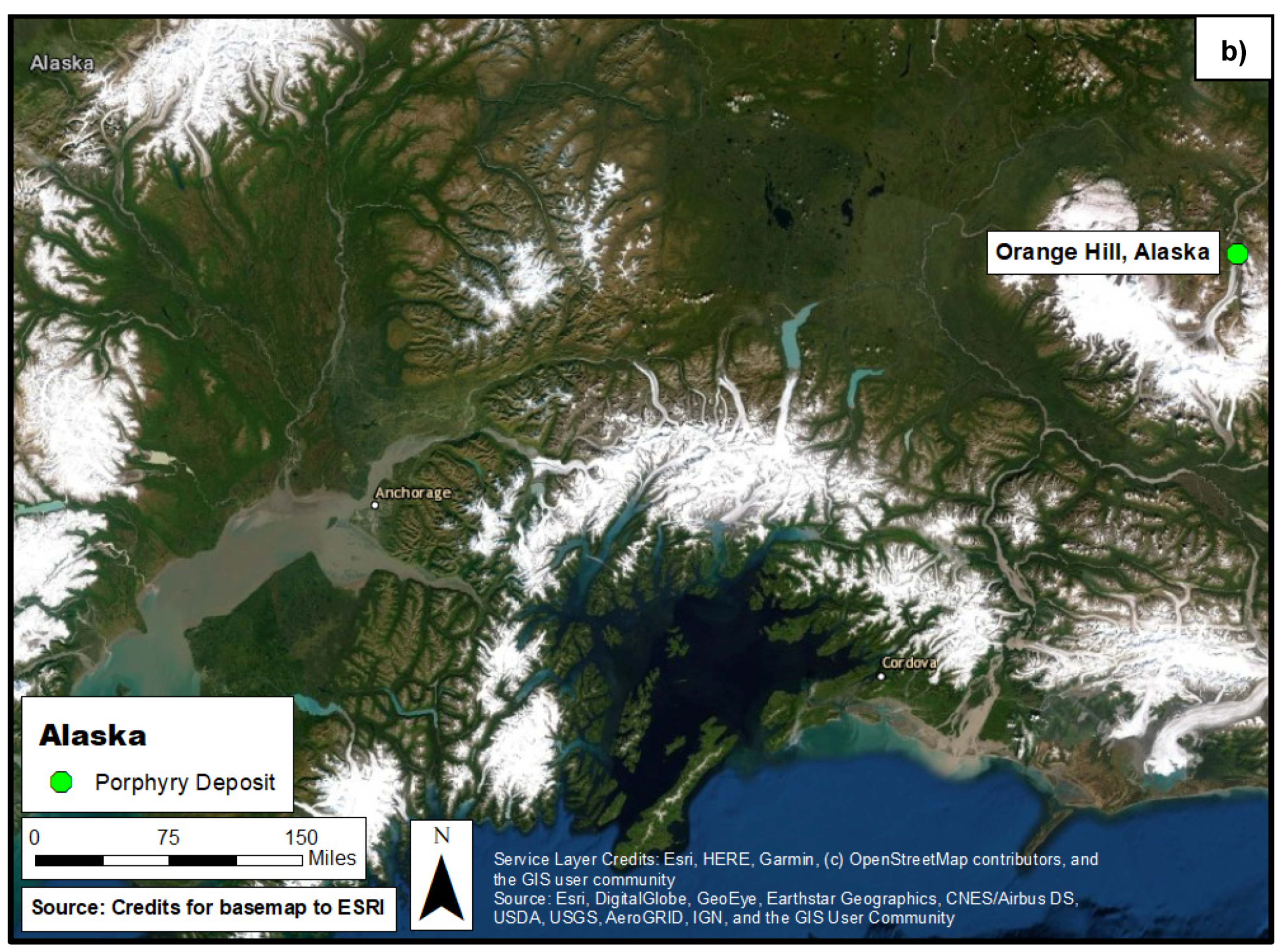
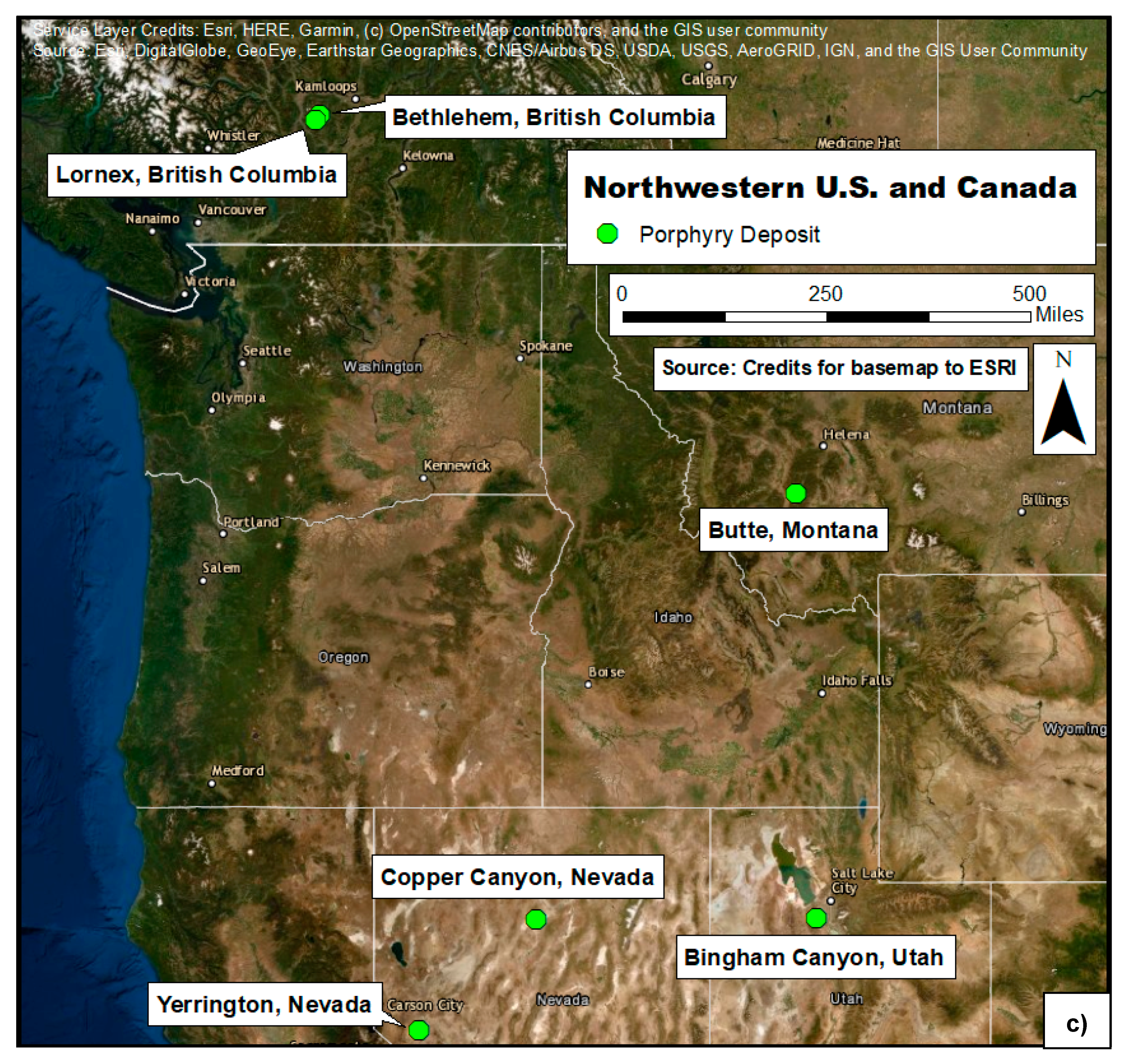
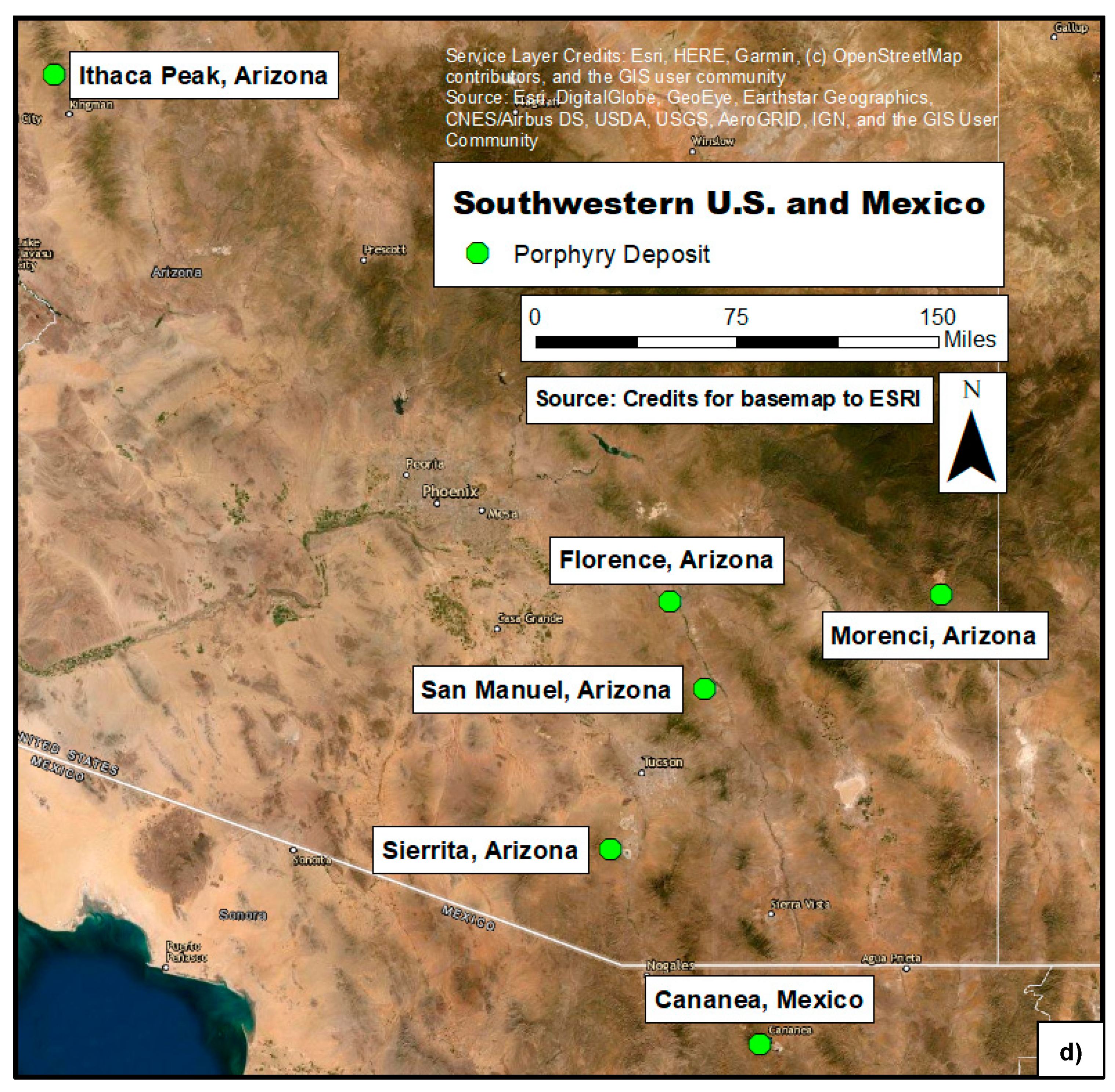
Figure 1.
Maps of deposit locations in western North America that were sampled. (a) Overall geologic map of the Western Cordillera (map constructed in ArcGIS). (b) Satellite image of the Orange Hill deposit in Alaska. (c) Satellite image of the British Columbian, Nevadan, Montanan, and Utahan deposits. (d) Satellite image of Arizonan and Mexican deposits.


Figure 2.
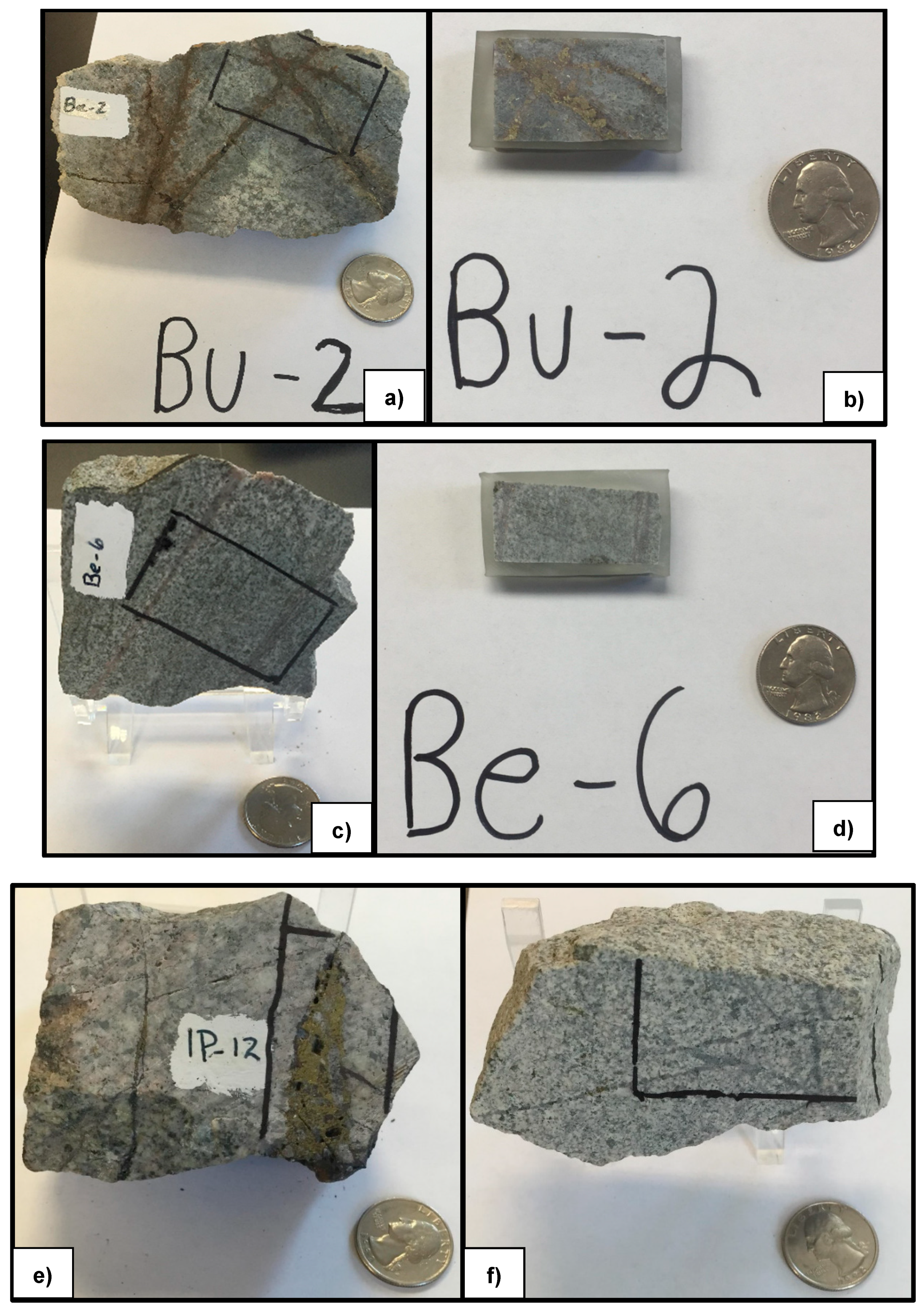
Example photographs of two samples from this study. (a) Bu-2 (Butte, Montana) hand sample showing sulfide vein stockwork characteristic of porphyry-type deposits and alteration haloes surrounding the veins. (b) Thin section billet cut from the sample in (a) and impregnated with epoxy. (c) Be-6 (Bethlehem, British Columbia) hand sample showing sulfide vein stockwork characteristic of porphyry-type deposits and alteration adjacent to the veins. (d) Thin section billet cut from the sample in (c) and impregnated with epoxy. (e) IP-12 (Ithaca Peak, Utah) hand sample showing a high-grade vein of Cu-Fe sulfides. (f) Y-3 (Yerington, Nevada) somewhat brecciated hand sample showing cross-cutting veinlet stockwork formed in multiple generations of fractures. American quarter for scale (~2.43 cm in diameter). Locations to be cut for thin-sectioning are outlined in black marker.
Figure 2.
Example photographs of two samples from this study. (a) Bu-2 (Butte, Montana) hand sample showing sulfide vein stockwork characteristic of porphyry-type deposits and alteration haloes surrounding the veins. (b) Thin section billet cut from the sample in (a) and impregnated with epoxy. (c) Be-6 (Bethlehem, British Columbia) hand sample showing sulfide vein stockwork characteristic of porphyry-type deposits and alteration adjacent to the veins. (d) Thin section billet cut from the sample in (c) and impregnated with epoxy. (e) IP-12 (Ithaca Peak, Utah) hand sample showing a high-grade vein of Cu-Fe sulfides. (f) Y-3 (Yerington, Nevada) somewhat brecciated hand sample showing cross-cutting veinlet stockwork formed in multiple generations of fractures. American quarter for scale (~2.43 cm in diameter). Locations to be cut for thin-sectioning are outlined in black marker.

Figure 3.
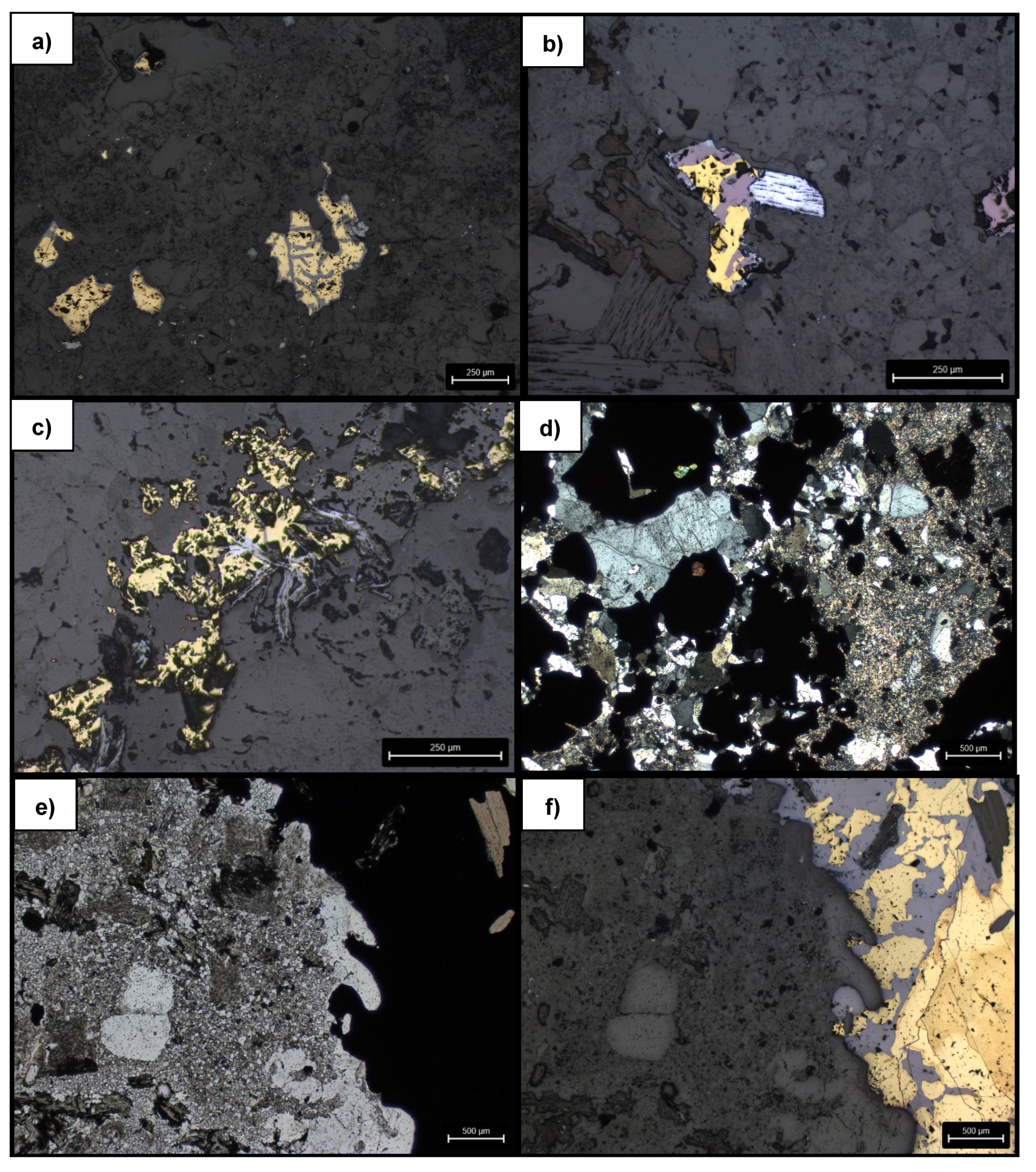
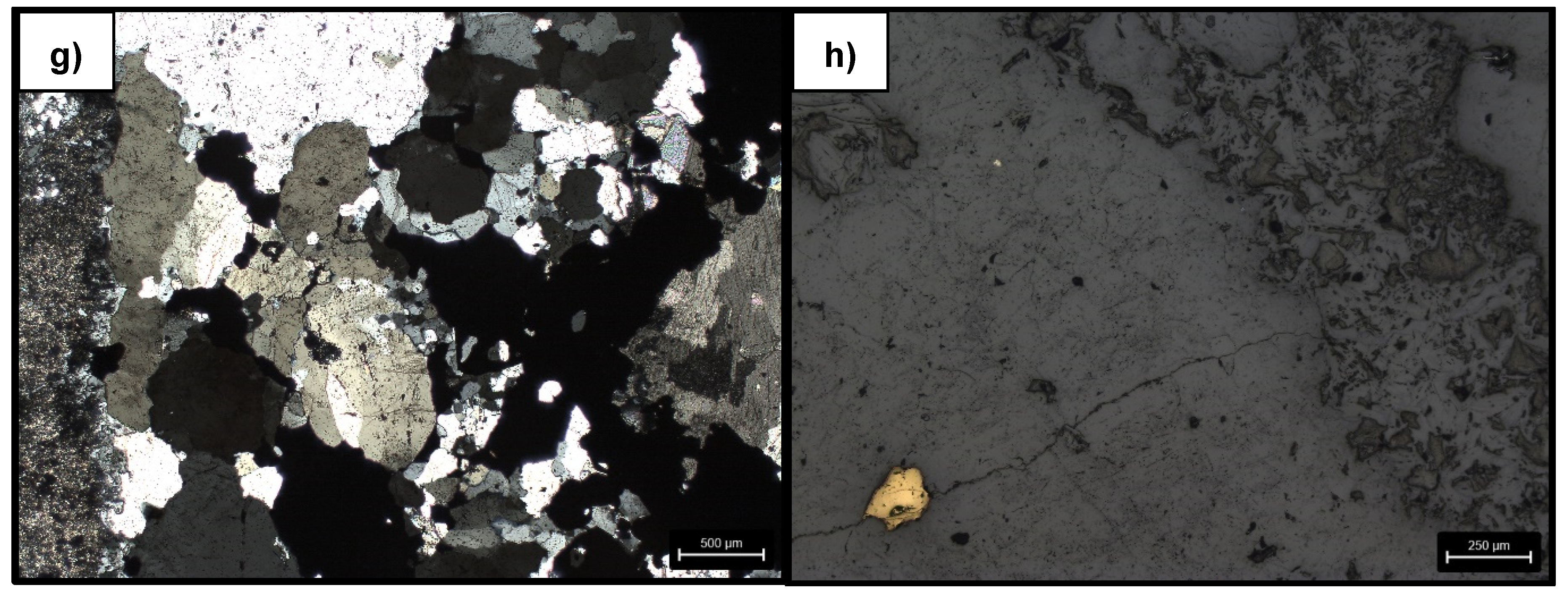
Example photomicrographs of two samples from this study. (a) Bi-2, chalcopyrite with alteration to chalcocite/covellite along crystal rims and fractures. Surrounding phases are quartz and sericite. RPPL (reflected plane-polarized light). (b) Bi-3, chalcopyrite, bornite, and molybdenite intergrown. Digenite alteration along the bornite and chalcopyrite crystal rims. Surrounding phases are biotite, quartz, and sericite. RPPL. (c) S-2, chalcopyrite and molybdenite in a quartz vein. RPPL (d) Bu-6, large pyrite crystals (some with possible zircon inclusions) in quartz + sericite + orthoclase. TXPL (transmitted cross-polarized light). (e) IP-12, vein of chalcopyrite + bornite + biotite in sericitized and chloritized porphyritic biotite quartz monzonite/latite. TPPL (transmitted plane-polarized light). (f) Same view as in (e), but in RPPL. (g) F-3, quartz + pyrite + chalcopyrite + calcite vein in sericitized monzonite host. (h) L-1, small grains of chalcopyrite (lower left) and molybdenite (upper right) in quartz and sericite. RPPL.
Figure 3.
Example photomicrographs of two samples from this study. (a) Bi-2, chalcopyrite with alteration to chalcocite/covellite along crystal rims and fractures. Surrounding phases are quartz and sericite. RPPL (reflected plane-polarized light). (b) Bi-3, chalcopyrite, bornite, and molybdenite intergrown. Digenite alteration along the bornite and chalcopyrite crystal rims. Surrounding phases are biotite, quartz, and sericite. RPPL. (c) S-2, chalcopyrite and molybdenite in a quartz vein. RPPL (d) Bu-6, large pyrite crystals (some with possible zircon inclusions) in quartz + sericite + orthoclase. TXPL (transmitted cross-polarized light). (e) IP-12, vein of chalcopyrite + bornite + biotite in sericitized and chloritized porphyritic biotite quartz monzonite/latite. TPPL (transmitted plane-polarized light). (f) Same view as in (e), but in RPPL. (g) F-3, quartz + pyrite + chalcopyrite + calcite vein in sericitized monzonite host. (h) L-1, small grains of chalcopyrite (lower left) and molybdenite (upper right) in quartz and sericite. RPPL.


Figure 4.
Plot of S content vs. sum of chalcophile elements determined by pXRF.

Figure 5.
Plots comparing the composition of samples determined by pXRF with those values calculated from mineral modes: (a) Cu, (b) Mo, (c) Fe, (d) S, (e) Si, (f) Al, (g) K, and (h) Mg. The grey, coarsely dashed lines show 1:1 equivalency for both methods.
Figure 5.
Plots comparing the composition of samples determined by pXRF with those values calculated from mineral modes: (a) Cu, (b) Mo, (c) Fe, (d) S, (e) Si, (f) Al, (g) K, and (h) Mg. The grey, coarsely dashed lines show 1:1 equivalency for both methods.

Figure 6.
Plot comparing Cu content of samples determined by pXRF with those values calculated from mineral modes but omitting high-Cu sample IP-12.
Figure 6.
Plot comparing Cu content of samples determined by pXRF with those values calculated from mineral modes but omitting high-Cu sample IP-12.


Table 1.
List of samples investigated in this study and their origins.
| Sample | Locality | Location | Sample | Locality | Location |
|---|---|---|---|---|---|
| Be-1 | Bethlehem | British Columbia | L-1 | Lornex | British Columbia |
| Be-4 | Bethlehem | British Columbia | Mo-2 | Morenci | Arizona |
| Be-6 | Bethlehem | British Columbia | Mo-4 | Morenci | Arizona |
| Bi-2 | Bingham Canyon | Utah | Mo-6 | Morenci | Arizona |
| Bi-3 | Bingham Canyon | Utah | Mo-8 | Morenci | Arizona |
| Bu-2 | Butte | Montana | OH-1 | Orange Hill | Alaska |
| Bu-6 | Butte | Montana | S-1 | Sierrita | Arizona |
| Bu-7 | Butte | Montana | S-2 | Sierrita | Arizona |
| C-3 | Cananea | Mexico | S-4 | Sierrita | Arizona |
| C-4 | Cananea | Mexico | SM-3 | San Manuel | Arizona |
| CC-1 | Copper Canyon | Nevada | SM-4 | San Manuel | Arizona |
| F-1 | Florence | Arizona | Y-3 | Yerington | Nevada |
| F-2 | Florence | Arizona | |||
| F-3 | Florence | Arizona | |||
| IP-1 | Ithaca Peak | Arizona | |||
| IP-2 | Ithaca Peak | Arizona | |||
| IP-3 | Ithaca Peak | Arizona | |||
| IP-10 | Ithaca Peak | Arizona | |||
| IP-12 | Ithaca Peak | Arizona |
Table 2.
Mineral modes (in volume%) of samples. Mineral abbreviations as in Whitney and Evans [25].
Table 2.
Mineral modes (in volume%) of samples. Mineral abbreviations as in Whitney and Evans [25].
| Sample: | Be-1 | Be-4 | Be-6 | Bi-2 | Bi-3 | Bu-2 | Bu-6 | Bu-7 | C-3 | C-4 | CC-1 | F-1 | F-2 | F-3 | IP-1 | IP-2 |
| Ccp | 0.3 | 1 | 1.5 | 1 | 1 | 0.5 | -- | 1.5 | -- | -- | 1 | 4 | 0.8 | 2.5 | -- | 0.1 |
| Cv | -- | -- | -- | 0.3 | -- | 0.2 | -- | 0.3 | -- | 2 | -- | -- | -- | -- | -- | 1 |
| Cct | -- | -- | -- | 1.5 | 0.1 | -- | 0.5 | -- | -- | -- | -- | -- | -- | -- | 0.5 | 0.5 |
| Bn | -- | 1 | 0.2 | 0.1 | 1 | -- | -- | -- | -- | -- | -- | -- | -- | -- | -- | -- |
| Dg | -- | -- | -- | -- | 0.3 | -- | -- | -- | -- | -- | -- | -- | -- | -- | -- | -- |
| Mol | -- | -- | -- | 0.2 | 0.1 | -- | -- | 0.5 | 0.5 | -- | -- | -- | -- | -- | -- | |
| Py | 1 | -- | -- | 2 | -- | 9 | 20 | 45 | 4 | 7 | -- | -- | 2 | 2 | 3 | 4 |
| Chl | 8 | 4.5 | 7 | 1 | -- | -- | -- | -- | -- | -- | -- | -- | 0.4 | 0.3 | -- | -- |
| Rt | 0.3 | -- | 0.3 | 0.5 | 0.2 | 1 | -- | -- | -- | -- | 0.3 | 0.5 | 1 | 0.4 | 1 | -- |
| Hem | 2 | 0.1 | -- | -- | -- | 3 | -- | -- | -- | 0.5 | -- | 0.5 | 0.5 | -- | -- | -- |
| Cal | -- | 2 | -- | -- | -- | -- | -- | -- | -- | -- | -- | -- | -- | 3 | -- | -- |
| Qz | 57.4 | 64.9 | 60 | 48.7 | 61.3 | 56.3 | 74.5 | 48.7 | 60.5 | 50 | 67 | 58 | 56.3 | 59.8 | 64.5 | 67.4 |
| Or | -- | -- | -- | -- | -- | -- | 3 | 10 | -- | -- | -- | |||||
| Ms | 27 | 25.5 | 22 | 42.7 | 25 | 30 | 2 | 4 | 35 | 40.5 | 23.7 | 34 | 12 | 32 | 31 | 27 |
| Bt | -- | 0.5 | -- | 1 | 10 | -- | -- | -- | -- | -- | 8 | 3 | 10 | -- | -- | -- |
| Pl | 3 | -- | 8 | -- | -- | -- | -- | -- | -- | -- | -- | -- | 5 | -- | -- | -- |
| Ap | 1 | 0.5 | 1 | 1 | 1 | -- | -- | -- | -- | -- | -- | -- | 2 | -- | -- | -- |
| Total | 100.0 | 100.0 | 100.0 | 100.0 | 100.0 | 100.0 | 100.0 | 100.0 | 100.0 | 100.0 | 100.0 | 100.0 | 100.0 | 100.0 | 100.0 | 100.0 |
| Sample: | IP-3 | IP-10 | IP-12 | L-1 | Mo-2 | Mo-4 | Mo-6 | Mo-8 | OH-1 | S-1 | S-2 | S-4 | SM-3 | SM-4 | Y-3 | |
| Ccp | 0.1 | 0.05 | 22 | 6 | 1 | -- | 2 | 1.5 | 1 | 1 | 2 | 0.5 | 3.5 | 4.5 | 2 | |
| Cv | 0.1 | 0.1 | -- | -- | -- | -- | -- | -- | -- | -- | -- | -- | -- | -- | -- | |
| Cct | -- | 0.2 | -- | -- | -- | -- | -- | -- | -- | -- | -- | -- | -- | -- | -- | |
| Bn | -- | -- | 10 | -- | -- | -- | -- | -- | -- | -- | -- | -- | -- | -- | -- | |
| Dg | -- | -- | -- | -- | -- | -- | -- | -- | -- | -- | -- | -- | -- | -- | -- | |
| Mol | 0.3 | -- | -- | 0.1 | -- | -- | -- | -- | -- | -- | 0.2 | 0.3 | -- | -- | -- | |
| Py | 1 | 9 | -- | -- | 5 | 2.5 | -- | 1.4 | 8 | 1.6 | 2 | 3 | 5 | 1 | -- | |
| Chl | -- | -- | 5 | -- | 13 | -- | 1.5 | -- | 11 | 11 | 2 | 0.5 | -- | -- | 4 | |
| Rt | 1 | -- | -- | -- | 1 | 0.3 | 0.3 | 0.2 | -- | 0.5 | 0.5 | 0.5 | 0.5 | 1.5 | 0.3 | |
| Hem | 1 | -- | 0.5 | -- | -- | -- | -- | -- | 0.5 | -- | -- | 0.3 | -- | 1 | 1.5 | |
| Cal | -- | -- | -- | -- | -- | -- | 0.3 | 0.9 | -- | -- | -- | 1 | -- | -- | -- | |
| Qz | 43.3 | 85.65 | 44.5 | 85.4 | 45 | 94.9 | 54.4 | 53.4 | 26.5 | 35 | 62.5 | 50.9 | 43 | 36.3 | 55.7 | |
| Or | 16 | -- | 1 | -- | -- | -- | -- | 7.1 | -- | 8.9 | 4 | 3 | -- | -- | 5 | |
| Ms | 10 | 5 | 12 | 8 | 34 | 2.3 | 34.5 | 33 | 15 | 10 | 25 | 36 | 37 | 26 | 25 | |
| Bt | 24.5 | -- | 1 | -- | -- | -- | 2 | 2.5 | 3 | -- | -- | -- | 4 | 25 | -- | |
| Pl | 1 | -- | 4 | -- | -- | -- | 5 | -- | 35 | 32 | 1.3 | 4 | 6.3 | 4 | 6 | |
| Ap | 1.7 | -- | -- | 0.5 | 1 | -- | -- | -- | -- | -- | 0.5 | -- | 0.7 | 0.7 | 0.5 | |
| Total | 100.0 | 100.0 | 100.0 | 100.0 | 100.0 | 100.0 | 100.0 | 100.0 | 100.0 | 100.0 | 100.0 | 100.0 | 100.0 | 100.0 | 100.0 |
Table 3.
Bulk rock compositions (elemental wt%) for selected elements calculated from modes determined by optical petrography.
Table 3.
Bulk rock compositions (elemental wt%) for selected elements calculated from modes determined by optical petrography.
| Sample | Be-1 | Be-4 | Be-6 | Bi-2 | Bi-3 | Bu-2 | Bu-6 | Bu-7 | C-3 | C-4 | CC-1 | F-1 | F-2 | F-3 | IP-1 | IP-2 |
| Mg | 1.2 | 0.8 | 1.0 | 0.3 | 1.6 | 0.0 | 0.0 | 0.0 | 0.0 | 0.0 | 1.3 | 0.5 | 1.6 | 0.0 | 0.0 | 0.0 |
| Al | 6.3 | 5.8 | 6.1 | 8.7 | 5.8 | 5.7 | 0.6 | 0.6 | 7.2 | 7.9 | 5.5 | 7.2 | 4.6 | 6.6 | 6.4 | 5.5 |
| Si | 32.3 | 35.5 | 35.4 | 30.2 | 34.5 | 28.9 | 30.4 | 16.5 | 33.9 | 29.2 | 37.0 | 33.4 | 33.8 | 33.2 | 35.0 | 35.1 |
| P | 0.2 | 0.1 | 0.2 | 0.2 | 0.2 | 0.0 | 0.0 | 0.0 | 0.0 | 0.0 | 0.0 | 0.0 | 0.4 | 0.0 | 0.0 | 0.0 |
| S | 1.1 | 1.0 | 0.9 | 3.4 | 1.2 | 8.4 | 17.4 | 33.2 | 4.2 | 7.5 | 0.5 | 2.1 | 2.3 | 3.2 | 3.1 | 4.6 |
| K | 2.7 | 2.6 | 2.2 | 4.2 | 3.5 | 2.8 | 0.5 | 0.3 | 3.5 | 3.8 | 3.2 | 3.7 | 3.5 | 3.2 | 3.1 | 2.7 |
| Ca | 0.5 | 1.0 | 1.0 | 0.4 | 0.5 | 0.0 | 0.0 | 0.0 | 0.0 | 0.0 | 0.0 | 0.0 | 1.3 | 1.2 | 0.0 | 0.0 |
| Ti | 0.3 | 0.0 | 0.3 | 0.4 | 0.2 | 0.8 | 0.0 | 0.0 | 0.0 | 0.0 | 0.3 | 0.5 | 0.9 | 0.4 | 0.9 | 0.0 |
| Fe | 1.9 | 1.4 | 1.6 | 2.3 | 1.4 | 10.9 | 15.0 | 28.5 | 3.3 | 6.2 | 1.1 | 2.7 | 3.5 | 3.1 | 2.5 | 3.4 |
| Cu | 0.2 | 1.7 | 1.0 | 3.3 | 2.3 | 0.4 | 0.7 | 0.8 | 0.0 | 2.1 | 0.5 | 2.1 | 0.4 | 1.3 | 0.8 | 2.0 |
| Mo | 0.0 | 0.0 | 0.0 | 0.2 | 0.1 | 0.0 | 0.0 | 0.4 | 0.6 | 0.0 | 0.0 | 0.0 | 0.0 | 0.0 | 0.0 | 0.0 |
| Balance | 53.5 | 50.1 | 50.2 | 46.2 | 48.7 | 42.0 | 35.4 | 19.6 | 47.3 | 43.2 | 50.5 | 47.9 | 47.8 | 47.7 | 48.2 | 46.7 |
| Sample | IP-3 | IP-10 | IP-12 | L-1 | Mo-2 | Mo-4 | Mo-6 | Mo-8 | OH-1 | S-1 | S-2 | S-4 | SM-3 | SM-4 | Y-3 | |
| Mg | 3.7 | 0.0 | 0.8 | 0.0 | 1.9 | 0.0 | 0.5 | 0.4 | 2.0 | 1.6 | 0.3 | 0.1 | 0.6 | 3.7 | 0.6 | |
| Al | 5.2 | 1.0 | 0.3 | 1.7 | 7.9 | 0.5 | 8.0 | 7.7 | 7.7 | 7.0 | 5.8 | 8.1 | 8.1 | 7.1 | 6.6 | |
| Si | 30.7 | 37.8 | 20.9 | 40.0 | 28.2 | 43.7 | 34.0 | 33.4 | 26.3 | 31.8 | 34.9 | 32.0 | 28.4 | 26.6 | 34.0 | |
| P | 0.3 | 0.0 | 0.0 | 0.1 | 0.2 | 0.0 | 0.0 | 0.0 | 0.0 | 0.0 | 0.1 | 0.0 | 0.1 | 0.1 | 0.1 | |
| S | 1.3 | 8.6 | 13.9 | 3.3 | 5.2 | 2.5 | 1.1 | 2.2 | 7.9 | 2.1 | 3.2 | 3.4 | 6.4 | 3.2 | 1.1 | |
| K | 5.4 | 0.5 | 1.2 | 0.8 | 3.3 | 0.2 | 3.7 | 4.5 | 1.7 | 2.2 | 3.0 | 3.9 | 3.9 | 4.8 | 3.2 | |
| Ca | 0.8 | 0.0 | 0.2 | 0.2 | 0.4 | 0.0 | 0.5 | 0.4 | 2.4 | 2.3 | 0.3 | 0.7 | 0.7 | 0.6 | 0.7 | |
| Ti | 0.9 | 0.0 | 0.0 | 0.0 | 0.9 | 0.3 | 0.3 | 0.2 | 0.0 | 0.5 | 0.5 | 0.5 | 0.4 | 1.3 | 0.3 | |
| Fe | 3.9 | 7.4 | 11.5 | 2.8 | 6.0 | 2.2 | 1.2 | 2.1 | 8.9 | 3.1 | 2.8 | 3.2 | 5.8 | 5.7 | 3.4 | |
| Cu | 0.2 | 0.5 | 19.7 | 3.2 | 0.5 | 0.0 | 1.1 | 0.8 | 0.5 | 0.5 | 1.0 | 0.3 | 1.7 | 2.2 | 1.1 | |
| Mo | 0.3 | 0.0 | 0.0 | 0.1 | 0.0 | 0.0 | 0.0 | 0.0 | 0.0 | 0.0 | 0.2 | 0.4 | 0.0 | 0.0 | 0.0 | |
| Balance | 47.2 | 44.3 | 31.5 | 47.8 | 45.5 | 50.6 | 49.7 | 48.5 | 42.7 | 48.8 | 47.8 | 47.6 | 43.7 | 44.8 | 49.1 |
Table 4.
Bulk rock compositions (elemental wt%) for selected elements determined by the average of point analyses for each thin section billet. Uncertainties are the averaged instrumental population standard deviation determined by the pXRF software: (2σ)inst and the sample standard deviation of the spot analyses across the billet: (s)spot. Samples with more than three spots analyzed are Bu-7 (five spots), Bu-2 (four spots), and IP-3 (four spots).
| Sample | Be-1 | Be-4 | Be-6 | Bi-2 | Bi-3 | Bu-2 | Bu-6 | Bu-7 | C-3 | C-4 | CC-1 | F-1 | F-2 | F-3 | IP-1 | IP-2 |
| Mg | 0.558 | 0.422 | 0.921 | 0.610 | 0.776 | 0.332 | 0.000 | 0.000 | 0.000 | 0.328 | 0.559 | 0.141 | 0.851 | 0.151 | 0.000 | 0.000 |
| Mg(2σ)inst | 0.197 | 0.201 | 0.203 | 0.284 | 0.237 | 0.668 | 0.409 | 1.405 | 0.318 | 0.356 | 0.209 | 0.326 | 0.213 | 0.391 | 0.327 | 0.437 |
| Mg(s)spot | 0.306 | 0.081 | 0.470 | 0.107 | 0.088 | 0.423 | 0.000 | 0.000 | 0.000 | 0.294 | 0.247 | 0.244 | 0.488 | 0.262 | 0.000 | 0.000 |
| Al | 5.995 | 5.798 | 5.979 | 6.977 | 6.007 | 5.821 | 0.134 | 0.152 | 6.972 | 6.819 | 5.109 | 4.832 | 4.397 | 5.828 | 5.247 | 4.555 |
| Al(2σ)inst | 0.134 | 0.136 | 0.130 | 0.173 | 0.147 | 0.185 | 0.076 | 0.197 | 0.153 | 0.163 | 0.131 | 0.121 | 0.119 | 0.156 | 0.127 | 0.123 |
| Al(s)spot | 0.131 | 2.363 | 0.659 | 0.077 | 0.646 | 0.348 | 0.134 | 0.147 | 0.954 | 0.641 | 0.215 | 1.550 | 0.357 | 1.631 | 2.394 | 0.411 |
| Si | 36.175 | 41.352 | 32.875 | 33.531 | 37.622 | 34.213 | 49.225 | 23.243 | 39.127 | 36.880 | 40.978 | 38.249 | 40.287 | 40.416 | 41.148 | 36.948 |
| Si(2σ)inst | 0.213 | 0.207 | 0.215 | 0.201 | 0.209 | 0.208 | 0.182 | 0.137 | 0.220 | 0.198 | 0.217 | 0.210 | 0.232 | 0.196 | 0.208 | 0.187 |
| Si(s)spot | 1.925 | 7.025 | 1.674 | 1.190 | 0.584 | 7.114 | 2.716 | 20.339 | 2.561 | 2.991 | 1.034 | 2.019 | 3.793 | 6.274 | 5.434 | 5.187 |
| P | 0.085 | 0.110 | 0.201 | 0.372 | 0.150 | 0.071 | 0.015 | 0.000 | 0.000 | 0.020 | 0.000 | 0.000 | 0.085 | 0.000 | 0.080 | 0.000 |
| P(2σ)inst | 0.020 | 0.023 | 0.019 | 0.026 | 0.023 | 0.035 | 0.045 | 0.070 | 0.033 | 0.033 | 0.039 | 0.029 | 0.026 | 0.041 | 0.024 | 0.038 |
| P(s)spot | 0.047 | 0.018 | 0.045 | 0.100 | 0.079 | 0.057 | 0.027 | 0.000 | 0.000 | 0.034 | 0.000 | 0.000 | 0.075 | 0.000 | 0.012 | 0.000 |
| S | 0.136 | 0.581 | 0.472 | 2.778 | 0.564 | 12.577 | 8.156 | 39.920 | 1.933 | 6.521 | 0.056 | 0.903 | 0.885 | 3.250 | 4.570 | 6.029 |
| S(2σ)inst | 0.008 | 0.014 | 0.012 | 0.036 | 0.015 | 0.100 | 0.064 | 0.451 | 0.028 | 0.060 | 0.007 | 0.017 | 0.018 | 0.037 | 0.045 | 0.052 |
| S(s)spot | 0.155 | 0.625 | 0.127 | 0.470 | 0.187 | 12.607 | 0.753 | 23.920 | 0.798 | 2.363 | 0.006 | 0.425 | 0.596 | 1.270 | 3.526 | 5.011 |
| K | 2.768 | 3.145 | 1.272 | 8.525 | 7.306 | 3.381 | 0.030 | 0.028 | 4.740 | 3.737 | 5.275 | 4.364 | 1.939 | 6.701 | 3.242 | 3.886 |
| K(2σ)inst | 0.041 | 0.039 | 0.034 | 0.083 | 0.069 | 0.063 | 0.010 | 0.036 | 0.055 | 0.051 | 0.056 | 0.044 | 0.039 | 0.064 | 0.042 | 0.044 |
| K(s)spot | 0.484 | 1.162 | 0.140 | 0.160 | 0.781 | 0.502 | 0.005 | 0.043 | 0.493 | 0.246 | 0.651 | 3.827 | 1.012 | 1.825 | 1.416 | 0.881 |
| Ca | 1.410 | 1.282 | 1.086 | 0.137 | 0.231 | 0.021 | 0.009 | 0.014 | 0.054 | 0.080 | 0.460 | 0.599 | 1.185 | 0.341 | 0.000 | 0.028 |
| Ca(2σ)inst | 0.034 | 0.029 | 0.030 | 0.026 | 0.023 | 0.027 | 0.004 | 0.019 | 0.016 | 0.017 | 0.024 | 0.022 | 0.032 | 0.025 | 0.026 | 0.014 |
| Ca(s)spot | 0.529 | 0.276 | 0.077 | 0.029 | 0.088 | 0.024 | 0.000 | 0.019 | 0.006 | 0.010 | 0.135 | 0.247 | 0.168 | 0.210 | 0.000 | 0.007 |
| Ti | 0.262 | 0.113 | 0.448 | 0.414 | 0.228 | 0.336 | 0.000 | 0.000 | 0.429 | 0.201 | 0.087 | 0.070 | 0.594 | 0.042 | 0.068 | 0.034 |
| Ti(2σ)inst | 0.088 | 0.059 | 0.105 | 0.115 | 0.083 | 0.179 | 0.062 | 0.163 | 0.094 | 0.092 | 0.083 | 0.080 | 0.109 | 0.102 | 0.101 | 0.082 |
| Ti(s)spot | 0.155 | 0.017 | 0.086 | 0.026 | 0.146 | 0.224 | 0.000 | 0.000 | 0.027 | 0.035 | 0.083 | 0.121 | 0.331 | 0.073 | 0.118 | 0.058 |
| Fe | 2.187 | 1.012 | 2.561 | 1.187 | 0.760 | 8.580 | 2.783 | 20.806 | 1.311 | 3.047 | 1.207 | 0.726 | 2.522 | 2.053 | 1.887 | 1.657 |
| Fe(2σ)inst | 0.031 | 0.024 | 0.033 | 0.027 | 0.024 | 0.066 | 0.029 | 0.422 | 0.026 | 0.035 | 0.026 | 0.023 | 0.033 | 0.029 | 0.029 | 0.027 |
| Fe(s)spot | 1.083 | 0.158 | 0.304 | 0.210 | 0.169 | 5.749 | 0.373 | 15.386 | 0.483 | 0.597 | 0.116 | 0.324 | 1.217 | 0.811 | 1.088 | 1.582 |
| Cu | 0.027 | 0.442 | 0.212 | 1.658 | 0.445 | 0.019 | 0.273 | 0.414 | 0.064 | 0.186 | 0.309 | 0.257 | 0.063 | 0.664 | 0.006 | 0.674 |
| Cu(2σ)inst | 0.002 | 0.006 | 0.005 | 0.016 | 0.007 | 0.002 | 0.005 | 0.014 | 0.003 | 0.005 | 0.005 | 0.005 | 0.003 | 0.008 | 0.002 | 0.007 |
| Cu(s)spot | 0.034 | 0.632 | 0.032 | 0.513 | 0.116 | 0.010 | 0.069 | 0.262 | 0.019 | 0.045 | 0.061 | 0.115 | 0.040 | 0.439 | 0.006 | 1.114 |
| Mo | 0.000 | 0.000 | 0.000 | 0.005 | 0.000 | 0.000 | 0.000 | 0.002 | 0.000 | 0.000 | 0.000 | 0.000 | 0.000 | 0.002 | 0.005 | 0.043 |
| Mo(2σ)inst | 0.002 | 0.002 | 0.002 | 0.001 | 0.002 | 0.002 | 0.002 | 0.002 | 0.002 | 0.002 | 0.002 | 0.002 | 0.002 | 0.002 | 0.002 | 0.001 |
| Mo(s)spot | 0.000 | 0.000 | 0.000 | 0.002 | 0.000 | 0.000 | 0.000 | 0.003 | 0.000 | 0.000 | 0.000 | 0.000 | 0.000 | 0.003 | 0.008 | 0.042 |
| balance | 50.397 | 45.743 | 53.974 | 43.805 | 45.910 | 34.650 | 39.374 | 15.422 | 45.370 | 42.181 | 45.960 | 49.860 | 47.192 | 40.553 | 43.746 | 46.146 |
| Sample | IP-3 | IP-10 | IP-12 | L-1 | Mo-2 | Mo-4 | Mo-6 | Mo-8 | OH-1 | S-1 | S-2 | S-4 | SM-3 | SM-4 | Y-3 | |
| Mg | 3.466 | 0.000 | 0.000 | 0.061 | 0.269 | 0.000 | 0.377 | 0.303 | 1.051 | 1.292 | 0.202 | 0.595 | 0.497 | 2.504 | 0.646 | |
| Mg(2σ)inst | 0.349 | 0.460 | 1.146 | 0.201 | 0.261 | 0.243 | 0.273 | 0.307 | 0.357 | 0.317 | 0.440 | 0.261 | 0.287 | 0.401 | 0.208 | |
| Mg(s)spot | 2.952 | 0.000 | 0.000 | 0.106 | 0.233 | 0.000 | 0.327 | 0.270 | 0.493 | 0.421 | 0.350 | 0.166 | 0.038 | 0.410 | 0.315 | |
| Al | 3.792 | 0.630 | 2.089 | 0.516 | 7.597 | 0.552 | 5.698 | 6.713 | 5.670 | 7.591 | 4.372 | 6.134 | 7.896 | 8.039 | 4.013 | |
| Al(2σ)inst | 0.132 | 0.075 | 0.153 | 0.058 | 0.165 | 0.066 | 0.148 | 0.167 | 0.167 | 0.187 | 0.150 | 0.156 | 0.182 | 0.212 | 0.114 | |
| Al(s)spot | 2.270 | 0.657 | 3.105 | 0.802 | 0.232 | 0.072 | 3.146 | 0.808 | 0.968 | 0.344 | 0.426 | 0.395 | 0.254 | 0.424 | 0.729 | |
| Si | 33.855 | 42.872 | 27.146 | 46.957 | 39.581 | 53.778 | 39.729 | 36.751 | 29.638 | 32.075 | 36.292 | 36.938 | 34.163 | 28.977 | 38.218 | |
| Si(2σ)inst | 0.226 | 0.176 | 0.167 | 0.210 | 0.227 | 0.228 | 0.205 | 0.204 | 0.182 | 0.216 | 0.203 | 0.202 | 0.187 | 0.243 | 0.212 | |
| Si(s)spot | 10.773 | 6.181 | 4.108 | 4.859 | 0.925 | 2.258 | 7.880 | 3.732 | 4.311 | 1.404 | 1.954 | 2.825 | 0.809 | 1.918 | 0.839 | |
| P | 0.417 | 0.045 | 0.047 | 0.085 | 0.137 | 0.000 | 0.030 | 0.056 | 0.014 | 0.108 | 0.239 | 0.071 | 0.167 | 0.153 | 0.057 | |
| P(2σ)inst | 0.025 | 0.038 | 0.043 | 0.035 | 0.024 | 0.042 | 0.031 | 0.024 | 0.051 | 0.024 | 0.027 | 0.024 | 0.026 | 0.023 | 0.028 | |
| P(s)spot | 0.436 | 0.042 | 0.081 | 0.023 | 0.044 | 0.000 | 0.052 | 0.016 | 0.024 | 0.004 | 0.161 | 0.028 | 0.044 | 0.067 | 0.059 | |
| S | 1.424 | 11.951 | 21.206 | 0.825 | 2.322 | 2.969 | 0.866 | 3.018 | 11.947 | 3.284 | 5.937 | 4.012 | 7.376 | 1.453 | 0.323 | |
| S(2σ)inst | 0.023 | 0.080 | 0.150 | 0.014 | 0.031 | 0.033 | 0.018 | 0.037 | 0.091 | 0.041 | 0.057 | 0.041 | 0.064 | 0.027 | 0.011 | |
| S(s)spot | 1.185 | 8.437 | 6.641 | 0.642 | 0.295 | 3.238 | 0.515 | 1.362 | 8.311 | 0.953 | 1.410 | 3.240 | 0.765 | 0.552 | 0.197 | |
| K | 5.778 | 0.301 | 0.087 | 0.361 | 4.530 | 0.296 | 5.385 | 5.082 | 1.676 | 3.363 | 3.247 | 5.932 | 4.304 | 5.508 | 3.039 | |
| K(2σ)inst | 0.075 | 0.015 | 0.026 | 0.010 | 0.057 | 0.014 | 0.057 | 0.058 | 0.043 | 0.056 | 0.050 | 0.065 | 0.056 | 0.093 | 0.043 | |
| K(s)spot | 2.875 | 0.358 | 0.077 | 0.573 | 0.073 | 0.042 | 2.497 | 1.210 | 0.058 | 2.083 | 0.498 | 1.774 | 0.105 | 0.334 | 0.905 | |
| Ca | 0.558 | 0.007 | 0.032 | 0.011 | 0.257 | 0.030 | 2.443 | 2.069 | 2.309 | 3.203 | 2.203 | 0.888 | 1.359 | 0.498 | 0.729 | |
| Ca(2σ)inst | 0.033 | 0.009 | 0.012 | 0.004 | 0.022 | 0.005 | 0.044 | 0.043 | 0.054 | 0.062 | 0.046 | 0.034 | 0.039 | 0.040 | 0.026 | |
| Ca(s)spot | 0.624 | 0.012 | 0.014 | 0.001 | 0.082 | 0.003 | 0.892 | 1.472 | 0.387 | 0.719 | 0.473 | 0.402 | 0.696 | 0.085 | 0.215 | |
| Ti | 0.698 | 0.000 | 0.000 | 0.000 | 0.358 | 0.126 | 0.263 | 0.241 | 0.137 | 0.404 | 0.465 | 0.168 | 0.307 | 1.228 | 0.232 | |
| Ti(2σ)inst | 0.148 | 0.066 | 0.150 | 0.031 | 0.102 | 0.045 | 0.084 | 0.091 | 0.131 | 0.135 | 0.110 | 0.106 | 0.102 | 0.235 | 0.088 | |
| Ti(s)spot | 0.334 | 0.000 | 0.000 | 0.000 | 0.032 | 0.016 | 0.171 | 0.030 | 0.120 | 0.018 | 0.325 | 0.185 | 0.036 | 0.027 | 0.118 | |
| Fe | 3.156 | 4.299 | 11.918 | 0.498 | 2.275 | 0.856 | 1.167 | 2.134 | 6.721 | 4.254 | 2.922 | 2.792 | 3.619 | 8.000 | 3.543 | |
| Fe(2σ)inst | 0.039 | 0.037 | 0.089 | 0.018 | 0.034 | 0.023 | 0.026 | 0.031 | 0.055 | 0.045 | 0.036 | 0.035 | 0.037 | 0.066 | 0.037 | |
| Fe(s)spot | 2.385 | 3.306 | 1.197 | 0.247 | 0.097 | 0.986 | 0.576 | 0.828 | 2.205 | 0.253 | 1.337 | 1.392 | 0.222 | 0.907 | 1.221 | |
| Cu | 0.022 | 0.122 | 14.803 | 0.199 | 0.000 | 0.061 | 0.409 | 0.757 | 0.024 | 0.033 | 0.930 | 0.032 | 0.607 | 0.400 | 0.116 | |
| Cu(2σ)inst | 0.002 | 0.003 | 0.160 | 0.004 | 0.003 | 0.003 | 0.006 | 0.009 | 0.002 | 0.002 | 0.010 | 0.002 | 0.008 | 0.007 | 0.004 | |
| Cu(s)spot | 0.006 | 0.139 | 3.822 | 0.166 | 0.000 | 0.055 | 0.235 | 0.545 | 0.008 | 0.017 | 0.640 | 0.038 | 0.097 | 0.218 | 0.085 | |
| Mo | 0.273 | 0.065 | 0.000 | 0.009 | 0.000 | 0.000 | 0.007 | 0.008 | 0.009 | 0.000 | 0.000 | 0.034 | 0.002 | 0.001 | 0.000 | |
| Mo(2σ)inst | 0.003 | 0.001 | 0.002 | 0.002 | 0.002 | 0.002 | 0.001 | 0.001 | 0.001 | 0.002 | 0.002 | 0.001 | 0.001 | 0.002 | 0.002 | |
| Mo(s)spot | 0.372 | 0.069 | 0.000 | 0.016 | 0.000 | 0.000 | 0.004 | 0.006 | 0.006 | 0.000 | 0.000 | 0.005 | 0.002 | 0.002 | 0.000 | |
| balance | 46.561 | 39.708 | 22.672 | 50.479 | 42.674 | 41.333 | 43.625 | 42.867 | 40.805 | 44.392 | 43.190 | 42.405 | 39.705 | 43.238 | 49.085 |
© 2020 by the authors. Licensee MDPI, Basel, Switzerland. This article is an open access article distributed under the terms and conditions of the Creative Commons Attribution (CC BY) license (http://creativecommons.org/licenses/by/4.0/).
Share and Cite
MDPI and ACS Style
Gray, C.A.; Van Rythoven, A.D. A Comparative Study of Porphyry-Type Copper Deposit Mineralogies by Portable X-ray Fluorescence and Optical Petrography. Minerals 2020, 10, 431. https://doi.org/10.3390/min10050431
AMA Style
Gray CA, Van Rythoven AD. A Comparative Study of Porphyry-Type Copper Deposit Mineralogies by Portable X-ray Fluorescence and Optical Petrography. Minerals. 2020; 10(5):431. https://doi.org/10.3390/min10050431
Chicago/Turabian StyleGray, Connor A., and Adrian D. Van Rythoven. 2020. "A Comparative Study of Porphyry-Type Copper Deposit Mineralogies by Portable X-ray Fluorescence and Optical Petrography" Minerals 10, no. 5: 431. https://doi.org/10.3390/min10050431
Note that from the first issue of 2016, this journal uses article numbers instead of page numbers. See further details here.