
Maintenance of Intraspecific Diversity in Response to Species Competition and Nutrient Fluctuations


1
Marine Ecology, GEOMAR Helmholtz Centre for Ocean Research, 24105 Kiel, Germany
2
Aquatic Ecology Group, Department of Architecture, Design and Urban Planning, University of Sassari, 07100 Sassari, Italy
3
Faculty of Science and Engineering, Åbo Akademi University, 20520 Turku, Finland
*
Author to whom correspondence should be addressed.
Microorganisms 2022, 10(1), 113; https://doi.org/10.3390/microorganisms10010113
Submission received: 15 November 2021
/
Revised: 16 December 2021
/
Accepted: 29 December 2021
/
Published: 6 January 2022
(This article belongs to the Special Issue New Insights on Phytoplankton Morpho-Functional Traits)
Abstract
:Intraspecific diversity is a substantial part of biodiversity, yet little is known about its maintenance. Understanding mechanisms of intraspecific diversity shifts provides realistic detail about how phytoplankton communities evolve to new environmental conditions, a process especially important in times of climate change. Here, we aimed to identify factors that maintain genotype diversity and link the observed diversity change to measured phytoplankton morpho-functional traits Vmax and cell size of the species and genotypes. In an experimental setup, the two phytoplankton species Emiliania huxleyi and Chaetoceros affinis, each consisting of nine genotypes, were cultivated separately and together under different fluctuation and nutrient regimes. Their genotype composition was assessed after 49 and 91 days, and Shannon’s diversity index was calculated on the genotype level. We found that a higher intraspecific diversity can be maintained in the presence of a competitor, provided it has a substantial proportion to total biovolume. Both fluctuation and nutrient regime showed species-specific effects and especially structured genotype sorting of C. affinis. While we could relate species sorting with the measured traits, genotype diversity shifts could only be partly explained. The observed context dependency of genotype maintenance suggests that the evolutionary potential could be better understood, if studied in more natural settings including fluctuations and competition.
1. Introduction
Global biodiversity is threatened by five major drivers: habitat change, overexploitation, pollution, introduction of non-indigenous species, and climate change [1,2]. The consequences of biodiversity loss include lower stability of ecosystem functions and a reduced efficiency of communities to take up resources, build up biomass, and recycle nutrients [3]. As a part of biodiversity, genetic or intraspecific diversity has received little attention for a long time [4], although it has been shown to enhance ecosystem recovery [5] and was linked to physiological versatility and ecological resilience towards climatic stress [6]. The ecological effects of intraspecific diversity can be as high or even higher than species effects [7].
Phytoplankton are diverse, globally distributed, and build the base for most marine food webs [8]. They account for approximately half of global primary productivity [9], and are substantial drivers for biogeochemical cycles [10,11]. Phytoplankton diversity is an important factor in structuring marine ecosystems [12]. Climate change-induced sea surface warming results in enhanced stratification, restricting nutrient availability, which is a major driver for phytoplankton composition and biomass [13,14,15]. Future predictions for phytoplankton communities in more stratified open oceans often suspect that smaller phytoplankton will find themselves in positions of advantage due to their ability to effectively take up nutrients at low concentrations [16,17]. However, there is consideration that larger cells could also benefit from the multiple drivers of global change, making predictions about phytoplankton communities in future oceans a difficult task [18]. Predicting diversity changes remains especially difficult, as it not only relies on understanding species coexistence, but also depends on intraspecific diversity.
Since Hutchinson’s “paradox of the plankton”, researchers have been trying to explain how the observed species diversity in a system with limited resources can be maintained [19,20]. While many solutions have been proposed, understanding the underlying mechanisms of species coexistence is still an ongoing topic in community ecology [21,22,23,24]. Interspecific trait variation and associated trade-offs are commonly seen as essential for coexistence, as they represent niche differentiation among species [25,26]. Modern coexistence theory identified a balance between stabilization and differences in species’ competitive abilities, which is required for species to coexist [27,28,29]. Like interspecific trait variation, intraspecific trait variation has been shown to be omnipresent [30,31,32,33]. It can change species interactions and thereby promote or undermine species coexistence [34,35,36,37,38]. While results appear contradictory, it is the type of trait and the trade-off exhibiting intraspecific trait variation that determines the effect on species coexistence [39]. Less is known about the effects of interspecific competition on intraspecific diversity, although the effects of species on genetic diversity have been hypothesized [40].
Moreover, variability of environmental factors has been shown to promote species coexistence by temporal niche partitioning [41,42]. In particular, nutrient fluctuations can prevent competitive exclusion, and as such sustain coexistence of phytoplankton attributable to different nutrient uptake strategies [43,44,45]. Nevertheless, little is known about the effects of nutrient fluctuations on the maintenance of the associated genotype variability, which has been shown experimentally to decline rapidly, while two phytoplankton species stably coexisted at a regularly fluctuating nutrient regime in the long term [46]. Recently it has been found in yeast that nutrient fluctuations maintain higher genetic diversity than static environments [47].
As phytoplankton are largely structured by nutrient availability [21,48,49], traits important for nutrient acquisition and utilization as well as trade-offs between them facilitate the understanding and prediction of community structures [50,51]. Competitive strategies of nutrient acquisition in phytoplankton were proposed by Sommer [43]: affinity-adapted species with low half-saturation constants have an advantage under nutrient limitation, while nutrient repletion favors velocity-adapted species, which have a high maximum nutrient uptake velocity (Vmax) and a high maximum growth rate (µmax). While the use of a half-saturation constant as a measure of nutrient affinity has been heavily criticized and, as an alternative, the use of affinity α is recommended [52], the general classification of nutrient strategies still holds and is visible in bloom succession from diatoms to coccolithophores [53,54], typical representatives for the described velocity- and affinity-adapted strategies, respectively. Furthermore, among phytoplankton major taxonomic groups, Vmax scales with a two-thirds exponent of cell size based on the relationship of cell surface to cell volume scaling and enzyme kinetics [50]. Cell size has been described as a master trait in phytoplankton because of its scaling with many functional traits [55]. It spans dimensions of 4 to 5 orders of magnitude [56,57] and contributes to the enormous interspecific trait variation described in phytoplankton [50]. Moreover, some studies have also reported substantial intraspecific trait variation in phytoplankton cell size and traits relevant for nutrient acquisition, growth, and toxin production [58,59,60,61]. This large intraspecific trait variation suggests high potential for adaptation, which could compensate for lower fitness of phytoplankton in more adverse conditions [18], and for the same coexistence mechanisms to operate as on species level.
The main objective of this study was to uncover mechanisms maintaining intraspecific diversity in two globally important but fundamentally different marine phytoplankton species. The coccolithophore Emiliania huxleyi and the diatom Chaetoceros affinis are different in their morpho-functional traits, such as cell shape and size, and nutrient uptake-related traits that are reflected in different nutrient uptake strategies; we assumed that the nine genotypes of each species used in this study also show trait differences. To explain mechanistically the genotype sorting of the two species, we identified the morpho-functional traits cell size and Vmax of each genotype individually. With this knowledge, we aimed to assess the effects of interspecific competition, nutrient availability, and temporal fluctuations in nutrient availability on intraspecific diversity. More precisely, we wanted to know (i) whether intraspecific diversity of one species is dependent on the presence of a competing species, (ii) whether intraspecific diversity is dependent on different nutrient concentrations and limitations, and (iii) if additional variability in nutrient availability, represented by changing temporal windows for species or genotypes with either affinity or velocity specialization to thrive, can maintain a higher intraspecific diversity.
2. Materials and Methods
2.1. Study System and Laboratory Conditions
The populations and communities used in this study comprised species from two major groups of phytoplankton, coccolithophores (Emiliania huxleyi) and diatoms (Chaetoceros affinis). Both coccolithophores and diatoms are cosmopolitan bloomers, together contributing up to 50% of marine primary production [62,63]. However, their different nutrient-utilization strategies [43,64] are mirrored in the succession of blooms: whereas diatoms initiate and drive the early peak of a bloom by rapid uptake of nutrients followed by rapid growth, coccolithophores occur later in the succession when the nutrient concentration is already lowered and their high affinity is advantageous [53,54]. These different nutrient uptake strategies possibly enable the coexistence of E. huxleyi and C. affinis in microcosms (Figure S1), which mimic natural shifts in nutrient concentrations from replete to deplete conditions. From each species, we used nine genotypes that were isolated in 2014 and 2015 from waters near Gran Canary (for detail on the genotypes used, see [65]).
The experiments were carried out in 0.5 L polycarbonate bottles (Nalgene) filled with 660 mL sterile filtrated (0.2 µm) artificial seawater (35 salinity; after Kester [66]. The experiment was performed in a climate chamber at 21.9 ± 0.6 °C and settled on a rotating wheel to ensure mixing of their content. Light was supplied by a 17:7 LD cycle (3-h sunrise and sunset) with 299.6 ± 21.0 µmol m−2 s−1 at maximum light intensity.
2.2. Trait Measurements
The maximum uptake rate Vmax for nitrogen was determined for each genotype of Chaetoceros affinis and Emiliania huxleyi by applying a gradient of seven levels of nitrate concentrations while keeping phosphate constant (Table 1). The applied nutrient concentrations differed slightly between the species, as they were for example adjusted to avoid co-limitation of the diatom with silicate. Silicate was added in access to both species by applying an N:Si ratio of 4 and 0.6 in E. huxleyi and C. affinis, respectively. Each treatment combination of genotype with nitrate concentration was three-fold replicated, which resulted in 189 experimental units per species. Due to space limitation on the plankton wheel, the Vmax experiments for C. affinis and E. huxleyi took place at different times (October 2020 and March 2019, respectively).
In order to ensure maximal uptake, we conducted the experiment with genotypes starting at minimum nitrogen cell quotas (Qmin), i.e., with cells that were starved prior to the experimental onset. Nutrient concentrations in this acclimation batch cycle were 1.8 µmol L−1 P, 30 µmol L−1 N, and 40 µmol L−1 Si for C. affinis, and 1.5 µmol L−1 P, 15 µmol L−1 N, and 3.75 µmol L−1 Si for E. huxleyi. The acclimation batch cycle lasted 17 and 14 days in E. huxleyi and C. affinis, respectively. To account for the substantial difference in size between the species, starting volumes were adjusted. All genotypes of C. affinis were inoculated with 250 cells mL−1, while E. huxleyi genotypes started with 1000 cells mL−1. Throughout the 4 days of experiment, the individual growth of each culture was followed daily by cell counts and inorganic dissolved nutrients measurements. To quantify E. huxleyi abundance, a 1 mL sample was taken and analyzed with a flow cytometer (Beckman Coulter Gallios). The abundance of C. affinis was analyzed from 5 mL Lugol’s iodine solution fixed samples under inverted microscopes Axiovert 200 and Axio Observer A1 (Zeiss) in Utermöhl chambers. Inorganic dissolved nutrient samples were taken by filtering a 6 mL sample over prewashed 0.2 µm GF/F filters (Whatman) and analyzed using an autoanalyzer (Thermo Scientific Flash).
Specific uptake (V) for each genotype at a given nutrient concentration was determined by choosing the highest per capita nitrate uptake during the experiment. Nitrate uptake was measured as the loss of dissolved nitrate within one day by calculating the difference between nitrate concentrations measured at consecutive days, normalized by the mean number of cells present at those days. The highest per capita uptake rate took place in most replicates between experiment day one and experiment day two. To calculate Vmax of each genotype, the determined specific uptake rates were fitted to a Monod model by using the starting nitrate concentrations.
The size of each genotype was calculated after Hillebrand [67] from the diameter/ width and length measurements. To account for high variability in size within single C. affinis genotypes, we quantified the proportion of different size classes and measured the sizes of five cells per class and replicate. For E. huxleyi starvation prior the start of the trait measurements might result in considerably different cell sizes [68]. Consequently, the sizes of 15 cells per replicate were assessed at the start of the diversity experiment to facilitate a comparison of single genotype traits to resulting diversity shifts.
2.3. Diversity Experiment
2.3.1. Experimental Design and Setup
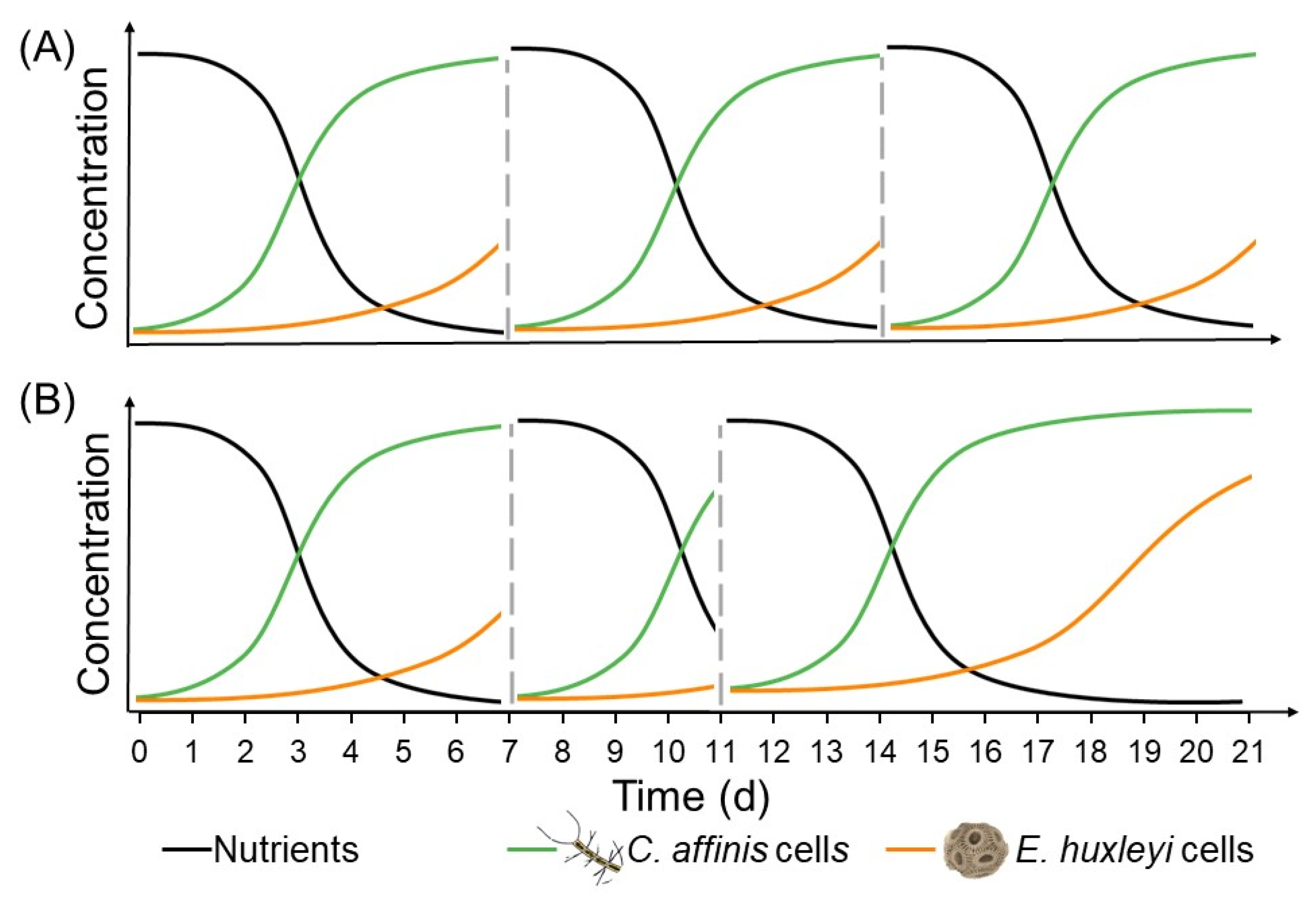
The effects of the presence of a competitor and fluctuations in nutrient availability on genotypic diversity were tested under different nutrient regimes using an experimental setup with the two phytoplankton species Emiliania huxleyi and Chaetoceros affinis. The two species were cultivated separately in mono-cultures and together in mix-cultures using a semi-continuous batch cycle system, where part of the community was transferred into new media to mark the start of a new batch cycle. To achieve the intended different nutrient fluctuations (regular versus irregular), the lengths of the batch cycles were varied (Figure 1). For half of the bottles, a part of the cells was transferred into new bottles with fresh media every 7 days (regular fluctuations at fixed batch cycle length), while for the other half a part of the cells was transferred after 7, 4, or 10 days (irregular fluctuations at variable batch cycle length), in a recurring fashion. Three different nutrient regimes were applied to reflect different N:P ratios and limitation scenarios in the ocean. Across these nutrient regimes, phosphate concentration was held equal with 0.93 ± 0.09 µmol L−1, while nitrate levels were adjusted to mimic a 10N:1P, 20N:1P, and 30N:1P ratio, and reached final nitrate concentrations of 8.60 ± 0.62, 19.08 ± 0.32, or 29.36 ± 0.47 µmol L−1, respectively. Silicate concentrations were aligned to reflect a 4:1 N:Si ratio. This relatively low N:Si ratio was chosen despite the potential of C. affinis to get co-limited by silicate, as preliminary tests of different nutrient concentrations demonstrated that this allowed for the longest coexistence of the model species in laboratory settings. Selenium, vitamins, and trace metals were also held constant according to f/8 concentration [69]. The culture treatment (mono-culture and mix-culture) was fully crossed with the batch cycle length treatment (fixed and variable) and the nutrient regimes (10N:1P, 20N:1P and 30N:1P), and replicated five times, resulting in 90 experimental units.
Prior to the experimental start, the genotypes were separately acclimated to experimental conditions with 20 µmol L−1 nitrate for 7 days. In the mix-culture, species were inoculated in concentrations of 25 cells mL−1 (C. affinis) and 500 cells mL−1 (E. huxleyi) to reflect similar biovolumes. The nine different genotypes of each species contributed equally to the total concentrations of the species. Mono-cultures were inoculated with 50 cells mL−1 (C. affinis) or 1000 cells mL−1 (E. huxleyi). The experiment ran for 91 days, or 13 batch cycles in total.
2.3.2. Sampling and Transfer
At the end of each batch cycle, bottles were sampled and transferred to the subsequent batch cycle under a biosafety cabinet (NuAire, model: NU-480-400E). For measurements of E. huxleyi density by a Gallios flow cytometer (Beckman Coulter), 3 mL volume was sampled over a 20 µm mesh-size sieve, which separated E. huxleyi cells from the significantly larger C. affinis. Another 5 mL were fixed with Lugol’s iodine solution for a cell count of C. affinis, and the cell size of both species was measured under inverted microscopes, as described above.
Part of the volume from the bottles with cells was transferred into new bottles with fresh media, marking the start of a new batch cycle. At first, transfer volumes for each culture and batch cycle length combination across all nutrient regimes were calculated, with the information on E. huxleyi density and one counted replicate each of C. affinis, to ensure a minimum initial density of 10 cells mL−1 of each species. With the start of the fifth batch cycle, the method was adjusted; transfer volumes were calculated individually for each nutrient treatment, and in the E. huxleyi mono-cultures for each bottle, to ensure that the starting densities in all treatments were comparable.
To follow the individual growth curve of each species during a batch cycle, in addition to the weekly sampling, the first long batch cycle (i.e., the third batch cycle) was characterized by daily measurements of cell density (E. huxleyi) and fluorescence (C. affinis) (Turner Designs, model: 10-AU Fluorometer). Nitrate, silicate, and phosphorus concentrations were measured at the end of the first three batch cycles in the mix-cultures at variable batch cycle length, to verify the proposed effects on nutrient concentrations at batch cycles of different lengths (Figure 1). Furthermore, nutrient concentrations in mix-cultures at the seventh batch cycle were measured daily from day 4 to day 7, to see which nutrient was the first to be completely taken up in each nutrient regime. The nutrient measurements were carried out in the same way as that described for the trait measurements.
2.3.3. Genotype Distribution
At midterm (i.e., 49 days or the seventh batch cycle) and at the end of the experiment (i.e., 91 days or the thirteenth batch cycle), subsamples were taken from each bottle to reisolate E. huxleyi and C. affinis cells for assessment of the genotype distribution, using microsatellites (after Hattich [65] and Listmann [46]; see the Supplementary Materials for details). Sequencing data were analyzed using GeneMarker software. Isolate genotypes were identified by comparing the primer peaks of the reisolates with the primer peaks of the stem culture genotypes. Experimental units with less than 5 isolates of one species identified were excluded from further analyses.
2.3.4. Shannon’s Diversity Index
Shannon’s diversity index H’ [70] was adapted on the genotype level and calculated separately for each species in every experimental unit, using the information on genotypes’ relative abundance. Calculation was carried out for both species separately to disentangle whether maintenance of intraspecific diversity varies between the species. The calculation (1) requires information about the number of genotypes S present, as well as their proportions pi, making Shannon’s diversity index H’ a comprehensive measure of diversity:
2.3.5. Statistical Analysis
Shannon’s diversity index and the relative abundances of the most frequent genotypes C91, C41, B82, B57, and B67 were analyzed by using mixed-effects models with four fixed factors: batch cycle length, nutrient regime, culture, and time. Bottle identity was incorporated as a random factor to account for repeated measures. Assumptions of tests were validated graphically, and the significance level for all analyses was set to p < 0.05. Starting from the most complex model (with all possible interactions), careful model simplification was applied. Model selection followed biological reasoning and the Bayesian information criterion (BIC). Final model output was reported as type II Wald F tests using Kenward-Roger df. Where test assumptions were not met, generalized linear mixed-effects models were used and reported as type II Wald χ2 tests.
3. Results
3.1. Trait Variability
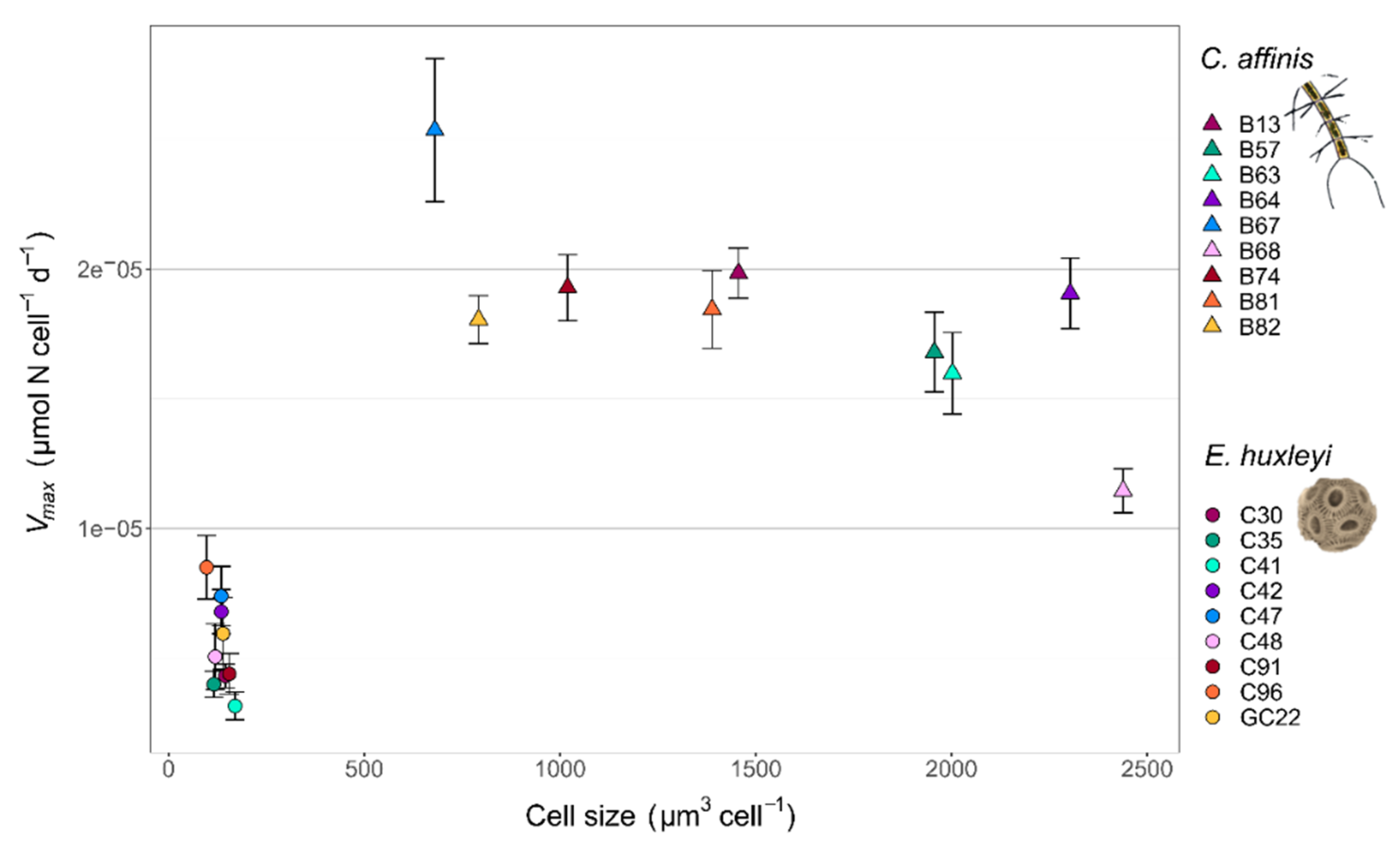
Trait measurements of Chaetoceros affinis and Emiliania huxleyi genotypes revealed fundamental trait differences between the two species and among the genotypes of each species, with regard to cell size and the maximum nutrient uptake rate Vmax (Figure 2). Between species, the generally smaller E. huxleyi genotypes had a mean cell size of 135 ± 20 µm3 in relation to the mean cell size of 1560 ± 612 µm3 for the larger C. affinis genotypes. In correlation with cell size, the mean Vmax was higher in C. affinis (1.8 × 10⁻⁵ ± 3.5 × 10⁻⁶ µmol N cell−1 d−1) than in E. huxleyi (5.5 × 10⁻⁶ ± 1.7 × 10⁻⁶ µmol N cell−1 d−1), showing the differences in nutrient uptake strategies of the species. In comparison, among the genotypes of each species, there was no correlation of Vmax with size. Intraspecific trait variability in E. huxleyi was reflected in a cell size range of 97 µm3 to 170 µm3 and a Vmax range of 3.1 × 10⁻⁶ µmol N cell−1 d−1 to 8.5 × 10⁻⁶ µmol N cell−1 d−1 in the genotypes. In the C. affinis genotypes, the sizes ranged from 680 µm3 to 2439 µm3 and Vmax ranged from 1.1 × 10⁻⁵ µmol N cell−1 d−1 to 2.5 × 10⁻⁵ µmol N cell−1 d−1. Standardized to the species mean, C. affinis showed higher variability in size (from −56% to 56%) compared to E. huxleyi (from −28% to 26%), whereas the variability in Vmax was higher in E. huxleyi (from −43% to 55%) than in C. affinis (from −37% to 39%).
3.2. Diversity Changes
3.2.1. Genotype Sorting
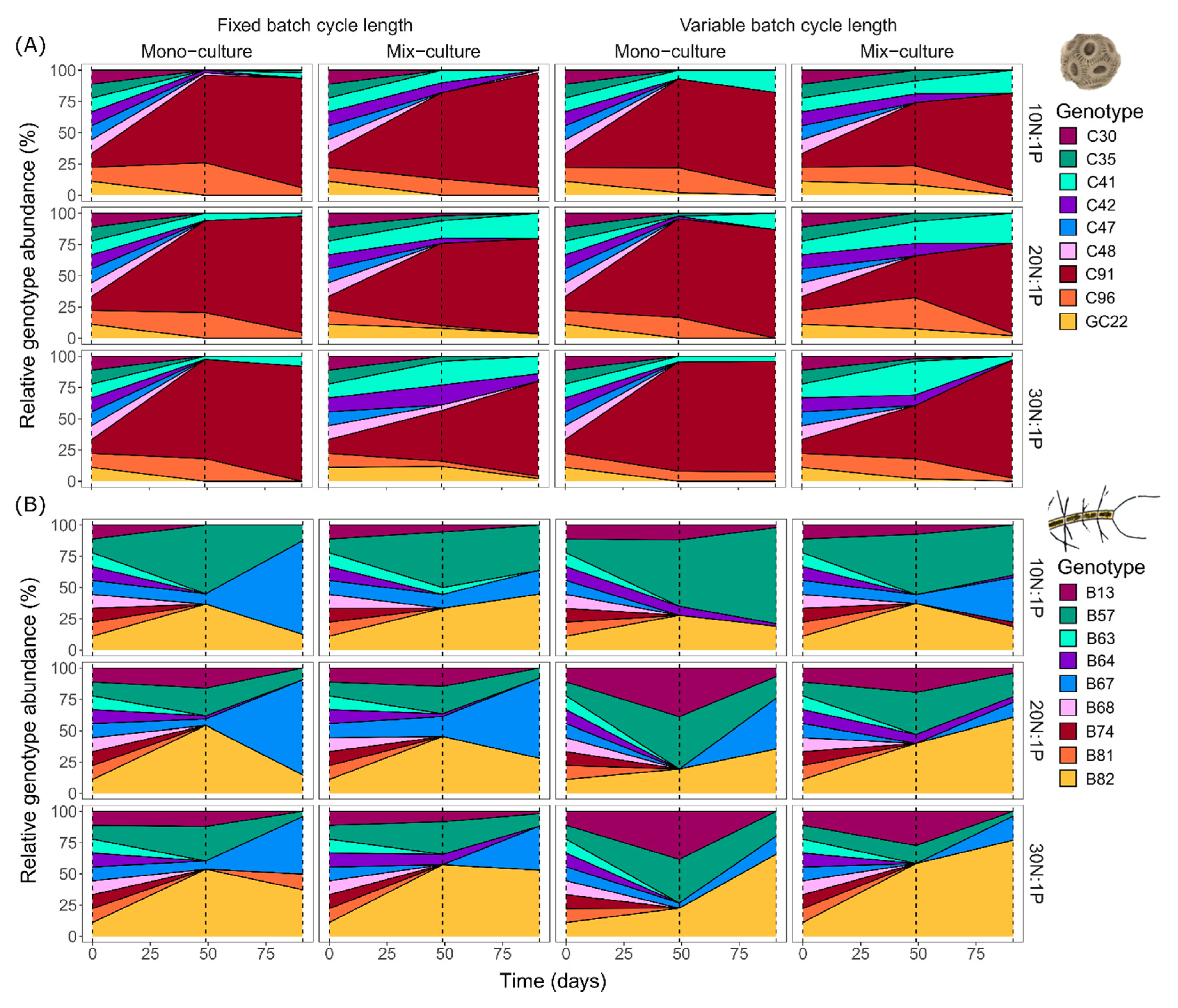
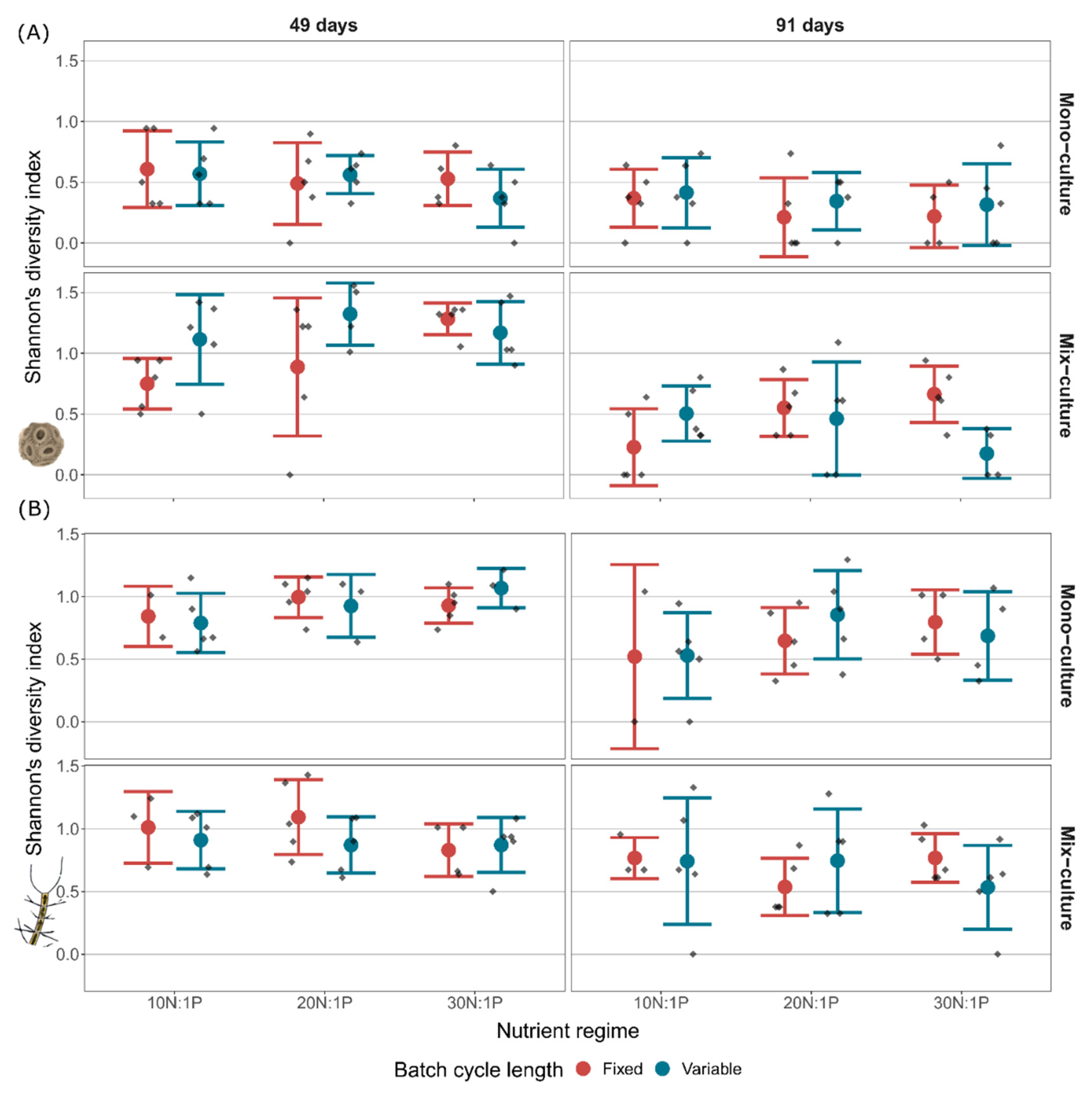
Genotype sorting of both E. huxleyi and C. affinis changed fundamentally over time (Figure 3), and the dynamics differed significantly between the two species. In E. huxleyi at midterm of the experiment, across all treatments, eight of the original nine genotypes were found. Their relative contributions to E. huxleyi total abundance changed drastically compared to the initial equal distribution, and led to dominance of genotype C91 in all treatments. Despite this uniform dominance, differences among treatments occurred in the maintenance of genotypes over time. The most prominent change is reflected in two more remaining genotypes in mix-cultures compared to mono-cultures. At the end of the experiment, the remaining genotypes were further reduced to six and the dominance of genotype C91 across all treatments increased even more, to nearly monodominance. In contrast to E. huxleyi, four genotypes majorly contributed to total C. affinis abundance throughout the experiment and dominated the different treatments in distinct ways. In addition, the two species differed in the exclusion process of genotypes; in C. affinis, this process was initially accelerated but in the longer term slower. More specifically, at midterm, a total of only six of the original nine genotypes were found, while at the end a total of seven genotypes were still present. Furthermore, the dominance of the single genotypes was not as pronounced as that described for E. huxleyi. This divergence in genotype sorting and exclusion between species is reflected in a 35% higher Shannon’s diversity index in C. affinis compared to E. huxleyi (Figure 4).
3.2.2. Maintenance of Intraspecific Diversity
Emiliania Huxleyi
In all treatments, the described change in genotype-sorting was reflected in a significant decrease of Shannon’s diversity index of E. huxleyi genotypes over time (Figure 4; “Time”, Table 2). The loss of Shannon’s diversity was, however, not uniform across treatments, but affected by culture, batch cycle length, and nutrient regime. Culture was especially important for the maintenance of Shannon’s diversity, as it was not only involved in several interactions, but mix-cultures generally increased diversity (“Culture”, Table 2), reflected in a 107% higher Shannon’s diversity in the mix-culture compared to mono-cultures at midterm. Coinciding with the higher Shannon’s diversity in mix-cultures, a reduction of the dominant genotype C91 (“Culture”, Table 3) and an increase of a subdominant genotype C41 (“Culture”, Table 4) were observed. Additionally, with rising nitrate concentration, Shannon’s diversity increased in mix-cultures but not in mono-cultures (“Culture × Nutrient”, Table 2). This increase in diversity correlated, once again, with a decrease in the proportion of genotype C91 (“Culture × Nutrient”, Table 3). Furthermore, batch cycle length affected Shannon’s diversity index through interactions (“Batch cycle length × Nutrient” and “Batch cycle length × Nutrient × Culture”, Table 2). More specifically, variable batch cycle length had no visible effect on diversity in mono-cultures at the end of the experiment, but led to 121% higher diversity compared to the fixed batch cycle length in the mix-cultures at the low nutrient regime 10N:1P. In contrast, variable batch cycle length decreased Shannon’s diversity index by 74% compared to the fixed batch cycle length at the high nutrient regime 30N:1P in the mix-cultures.
Chaetoceros Affinis
Shannon’s diversity index of C. affinis genotypes significantly decreased with time as a result of increased dominance of the four major contributing genotypes (Figure 4; “Time”, Table 5). Diversity was interactively affected by culture and nutrient regime (“Culture × Nutrient”, Table 5). This interaction was reflected in a 12% diversity decline from 10N:1P to 30N:1P in the mix-cultures compared to a 29% increase with the nutrient regime in the mono-cultures. The composition of C. affinis genotypes was largely structured by nutrients. The 20N:1P and 30N:1P nutrient regimes were dominated by genotype B82 (“Nutrient”, Table 6), while the 10N:1P regime was mainly composed of genotype B57 (“Nutrient”, Table 7). Variable batch cycle length led to a higher proportion of genotype B57 (“Batch cycle length”, Table 7), while fixed batch cycle length favored genotype B67 (“Batch cycle length”, Table 8). Additionally, genotype B67, which at midterm in some of the samples was below detection limit, increased with time in all treatments (“Time”, Table 8) and genotype B82 was more abundant in mix-cultures compared to mono-cultures (“Culture”, Table 6).
4. Discussion
Trait measurements of Emiliania huxleyi and Chaetoceros affinis genotypes indicated inter- and intraspecific trait variability with respect to size and the maximum nitrate uptake rate, Vmax. While E. huxleyi showed a higher percentage of variability in Vmax, C. affinis exhibited higher variability in size. The results of the diversity experiment showed that while genotype sorting of both species changed considerably over time, the patterns of the dynamics differed between species. As such, the genotype diversity of the two species was altered in different ways by the experimental treatments culture, batch cycle length, and nutrient regime. Shannon’s diversity in E. huxleyi was maintained by interspecific competition through the presence of C. affinis, and by irregular fluctuations in the 10N:1P nutrient regime, whereas C. affinis diversity was maintained by interspecific competition in the 10N:1P nutrient regime.
4.1. Maintenance of Intraspecific Diversity
4.1.1. Effects of Interspecific Competition
Our results showed that intraspecific diversity of one species can be affected by the presence of another and indicated that the coexistence of species might play an important role in the maintenance of intraspecific diversity. Interspecific competition could change intraspecific competition, resulting in higher intraspecific diversity. Specifically, the Shannon’s diversity of E. huxleyi was maintained for longer when cultivated together with C. affinis in a mix-culture compared to cultivation in a mono-culture. One possible explanation could be that the co-occurring growth of C. affinis effectively changed the nutrient concentrations or ratios, and by this process altered the competition between the E. huxleyi genotypes. As indicated by its higher cell size and Vmax, C. affinis (when compared to E. huxleyi) represents the better competitor for nutrients under replete nitrate conditions, and as such it likely altered the nutrient regime at the beginning of a batch cycle towards limiting to depleted conditions. In contrast to C. affinis, E. huxleyi is an affinity-adapted species, reflected in its smaller size and lower Vmax. As such, the rapid depletion of nutrients by the diatom at the onset of a batch cycle likely favored certain E. huxleyi genotypes and led to the decelerated exclusion speed of E. huxleyi genotypes. This could be regarded as an example of the facilitation described by Vellend, as shown in models to increase genotype richness as a result of higher species richness [76]. The observation also agrees with certain findings in a plant community, where maintenance of genetic variation was reported to depend on species diversity [77].
In C. affinis, the presence of the competitor altered Shannon’s diversity depending on nutrient conditions. Our results suggested that the effect of the interspecific competitor on diversity was mediated by species evenness, which in turn was driven by the nutrient regime (Figure S1). Evenness and as such the contribution of E. huxleyi to the total biovolume were highest in the 10N:1P nutrient regime. Only in the 10N:1P nutrient regime a positive effect of the presence of E. huxleyi could be measured. In the 30N:1P nutrient regime, the E. huxleyi biovolume contribution was negligible, and the influence of interspecific competition on the intraspecific diversity of C. affinis was highly unlikely. This suggests that the promotion of intraspecific diversity of a species requires substantial contribution of the competitor species to total biomass.
Furthermore, our results showed that genotype identity, which underlies intraspecific diversity, was altered by the presence of a competitor in both E. huxleyi and C. affinis. This was reflected, for example, by the higher relative abundances of genotypes C41 and B82 in mix-cultures compared to mono-cultures, respectively. Relative abundance shifts might have resulted from trait variability among genotypes, allowing for diverging responses to trait space shifts driven by interspecific competition. For example, in E. huxleyi mono-cultures, the higher Vmax of genotype C91 compared to C41 could have been beneficial. However, in the presence of C. affinis, with a much higher Vmax than E. huxleyi, nutrient availability for E. huxleyi likely decreased and therefore genotype C41 gained in terms of relative contribution. While it is known that intraspecific trait variation can change species’ interactions [34,35], our results underscore the hypothesized effects of species on genetic diversity [40].
4.1.2. Effects of Nutrient Fluctuations
As nutrient fluctuations can sustain species coexistence [43], we assumed that mechanisms of coexistence are the same on the genotype level and, therefore, additional variability promotes intraspecific diversity. Contrary to our expectations, the outcome from our work showed no generally higher intraspecific diversity when applying irregular rather than regular nutrient fluctuations, in the form of batch cycle length that changed nutrient availability (Figure S3). This outcome was especially surprising, considering that in yeast, nutrient fluctuations maintain higher genetic diversity than static environments [47]. These contradictory findings were likely to have been dependent on the different setups of fluctuations. First, with our fluctuation treatment, the quality and quantity of nutrients supplied was not altered. Second, in contrast to the cited studies that were conducted in chemostats [43,47], in our approach nutrient concentrations were allowed to shift from replete to deplete conditions in both fluctuation environments (Figure S4). Consequently, we did not apply a constant, static environment, but rather mimicked more natural conditions in our system, such as the occurrence and fluctuations in mixing events, which apparently resulted in a low effect of fluctuations on diversity.
Nevertheless, we found that for E. huxleyi only in the 10N:1P nutrient regime, variable batch cycle length led to higher Shannon’s diversity than did the fixed batch cycle length. As nitrate was the first nutrient to be depleted in the 10N:1P regime (Figure S4), this suggests that in our system, nitrate limitation was needed for irregular nutrient fluctuations to be of advantage. With respect to species level, it has been shown that nutrient fluctuations can increase macroalgae diversity in nutrient-limited coastal communities, while suppressing diversity in nutrient-enriched communities [78]. The authors explained their finding with the hump-shaped relationship between productivity and diversity [79], through which enrichment resulted in a diversity gain at low productivity sides and a loss in high productivity sides [80,81]. At first sight, our data verified this pattern at the genotypic level, and explained both the observed increase in genotype variation in E. huxleyi in the 10N:1P nutrient regime and the observed decline in genotype variation in the 20N:1P and 30N:1P nutrient regimes. Based on stoichiometry and confirmed by nutrient measurements (Figure S3), the 10N:1P regime represents a deplete regime and the 20N:1P and 30N:1P represent replete regimes, in terms of nitrate. However, considering phosphate levels, the 30N:1P regime would be a deplete regime, although the irregular fluctuations suppressed intraspecific diversity rather than promote it. As our fluctuating nutrients did not lead to enrichment but supplied the same amount of nutrients at different growth stages, it is likely that we did not observe a direct effect of a productivity-diversity relationship. However, an indirect effect in the mix-culture was possible, as the relative share of E. huxleyi in mix-cultures was significantly higher at 10N:1P than at 30N:1P (Figure S1), which might have prevented rare genotypes from being excluded. At 30N:1P, the very low abundance of E. huxleyi could have resulted in an increased likelihood of stochastic extinctions of genotypes, which was intensified by irregular fluctuations, presumably in the short batch cycles where the lowest E. huxleyi contribution occurred.
In our experiment, fluctuations did not affect the Shannon’s diversity of C. affinis, but did affect the remaining genotype identity. The fact that Shannon’s diversity was not affected by fluctuations could be due to the generally higher genotype diversity of C. affinis compared to E. huxleyi; in C. affinis, this resulted in a similar dominance pattern among treatments, however, with different genotypes. As such, Shannon’s diversity did not capture the observed genotype diversity shifts of C. affinis. Another potential explanation is that short, normal, and long batch cycles did not constitute a regulating force on the Shannon’s diversity of C. affinis because they all captured the end of growth or stationary phase that is reached on the fifth day (Figure S2). Furthermore, the long batch cycle of the irregular fluctuations did not impose a selection pressure on C. affinis as, contrary to our expectation, the long stationary phase did not result in senescence of C. affinis (Figure S1).
Irregular fluctuations promoted genotype B57, whereas regular fluctuations benefited genotype B67. As genotype B67 showed the highest Vmax of all genotypes, this could mean that the regular fluctuations favored genotypes that gained competitive advantage through a high Vmax. In contrast, the importance of being a good competitor due to high Vmax seemed lower at irregular fluctuations as the proportion of genotype B57 with a lower Vmax increased. This could be driven by the long batch cycle, where other traits such as affinity or storage capacity might have been more important. This shows that even small environmental differences resulting from irregular versus regular fluctuations can select for different genotypes that are specialized to a specific environment.
4.1.3. Effects of Nutrients
The role of nutrients on Shannon’s diversity remained concealed in interactions with the other treatments, as discussed. However, and specifically in C. affinis, genotype identity was structured by the nutrient regime. The considerably stronger effect of nutrient regimes on the genotype sorting of C. affinis compared to E. huxleyi was surprising, considering that (i) C. affinis was potentially co-limited by silicate across all nutrient regimes (Figure S4), and (ii) the C. affinis percentage trait variability in Vmax was smaller than that of E. huxleyi. Similar patterns were observed in a previous study, where the genotype sorting of C. affinis was more affected by CO2 concentration than was the genotype sorting of E. huxleyi (after 64 days; [46]), although the response variability in growth rate changes to CO2 was lower in C. affinis [65]. The authors discussed the overriding effects of general laboratory conditions on E. huxleyi genotype sorting, which likely also explain the dominance of the same E. huxleyi genotype across all treatments in this study. Only the relative abundance of E. huxleyi genotype C91 decreased with rising nitrate in the presence of C. affinis, thereby driving the according change in Shannon’s diversity. However, as this effect was only observable in competition with C. affinis, and the biomass of C. affinis increased with rising nitrate concentration (Figure S1), this indicates that C. affinis had a stronger effect on nutrient availability for E. huxleyi genotypes than did the nutrients provided at the start of a batch cycle.
Genotype sorting of C. affinis showed that the 20N:1P and 30N:1P nutrient regimes were dominated by genotype B82, while the 10N:1P regime was dominated by genotype B57. It is well known that higher Vmax found in diatoms are advantageous under high nutrient environments in relation to fundamental relationships such as cell surface to cell volume scaling and enzyme kinetics [50]. Trait measurements revealed that genotype B82 had a slightly higher Vmax than B57, indicating that a higher Vmax could be beneficial at higher nitrate concentrations. However, differences in Vmax between these C. affinis genotypes were small, and thus not sufficient to explain the genotype sorting. Additional trait measurements of Vmax for phosphate and silicate could have provided useful information, especially as they might also have been limiting. This applies particularly to potential phosphate limitation in the 30N:1P regime and silicate for C. affinis across treatments (Figure S4), potentially restricting the explanatory power of Vmax for nitrate. Cell size trait measurements do not explain genotype sorting at the different nutrient regimes, which could be caused by the absence of a correlation with Vmax among the genotypes. Vmax typically scales with phytoplankton cell size [64,82]; however, we found this relationship only between species. Similar patterns have been found for trade-offs between species that did not operate within species [39,83,84]. Moreover, the limited potential of trait measurements to explain genotype sorting is likely caused by the difference between the fundamental niche in absence of genotype and species competition and the realized ecological niche expressed under competition [85]. A quantitative study on the more than 60 year old concept supported the hypothesis that the fundamental niche is larger than the realized niche, and thereby underlines the importance of biotic interactions for species survival [86]. As genotypes show trait variability as well, this concept should also apply on the intraspecific level, and therefore lead to differences between fundamental and realized niches, restricting the explanatory power of individual trait measurements.
4.2. Implications for Phytoplankton in Future Oceans
Understanding the mechanisms by which genotypes coexist is an important step in grasping how biodiversity is maintained in nature. It provides realistic detail about the capability of communities to respond to new environments, a process especially important in times of global change. Our findings show that maintenance of intraspecific diversity is context-dependent, suggesting that the potential for species and communities to cope with altered conditions could be better understood, if it was studied in more natural settings including fluctuations and competition. In particular, the presence of a competitor showed pronounced direct effects on intraspecific diversity, in addition to the indirect modulation effects of other drivers. The competition effects were species-specific and depended on species composition, underlining the importance of assessing evolutionary change in response to new environmental conditions in an ecological context. Disentangling and understanding evolutionary change, and thus genotype sorting, in phytoplankton communities will help in assessing the potential for phytoplankton to cope with climate change, and ultimately improve predictions about their future. These predictions are essential, as shifts in phytoplankton can have cascading effects on ecosystems, which can eventually affect their services provided to humans [87].
Supplementary Materials
The following materials are available online at https://www.mdpi.com/article/10.3390/microorganisms10010113/s1, Figure S1: Stacked biovolume (mean ± SD) of E. huxleyi (orange) and C. affinis (green) at the end of each batch cycle over the course of time; Figure S2: Daily measurements of cell density of E. huxleyi (orange) and fluorescence of C. affinis (green) at batch cycle three under variable batch cycle length (long batch cycle); Figure S3: Measurements (mean ± SD) of nitrate (red), phosphate (green), and silicate (blue) at the end of batch cycles one (7 days), two (4 days) and three (10 days) under variable batch cycle length in mix-cultures; Figure S4: Measurements of nitrate (red), phosphate (green) and silicate (blue) in mix-cultures at batch cycle seven from day four to seven; Table S1: Primer sequences for microsatellite analysis.
Author Contributions
Conceptualization, J.H., G.S.I.H., S.P. and B.M.; methodology, J.H., G.S.I.H., S.P. and B.M.; formal analysis, J.H. and B.M.; investigation, J.H., G.S.I.H. and S.P.; data curation, J.H., G.S.I.H., S.P. and B.M.; writing—original draft preparation, J.H. and G.S.I.H.; writing—review and editing, J.H., G.S.I.H., S.P. and B.M.; visualization, J.H.; supervision, G.S.I.H. and B.M.; project administration, J.H., G.S.I.H. and B.M.; funding acquisition, B.M. All authors have read and agreed to the published version of the manuscript.
Funding
This research was funded by the DFG priority program SPP 1704 Dynatrait: Birte Matthiessen MA5058/2-2. The research stay of S.P. was funded by the German Academic Exchange Service (DAAD) and the Programma Mobilità Giovani Ricercatori of the University of Sassari (Italy).
Institutional Review Board Statement
Not applicable.
Informed Consent Statement
Not applicable.
Data Availability Statement
Data are available at PANGAEA (www.pangaea.de).
Acknowledgments
We thank T. Hansen, K. Qelaj, L. Hansen, J. Hoffmann, A. Fabricius, and V. Fey for their laboratory assistance, and our student assistants J. Houvener, S. Antoniello, J. Eberle, T. Liese, J. Romberg, J. Throm, and K. Seebass for their support. We further thank S. Marten, D. Gill, and T. Bayer for answering all questions related to the genetic lab work and analysis.
Conflicts of Interest
The authors declare no conflict of interest.
References
- Pereira, H.M.; Navarro, L.M.; Martins, I.S. Global biodiversity change: The bad, the good, and the unknown. Annu. Rev. Environ. Resour. 2012, 37, 25–50. [Google Scholar] [CrossRef] [Green Version]
- Díaz, S.; Settele, J.; Brondízio, E.S.; Ngo, H.T.; Guèze, M.; Agard, J.; Arneth, A.; Balvanera, P.; Brauman, K.; Butchart, S.H. Summary for policymakers of the global assessment report on biodiversity and ecosystem services of the intergovernmental science-policy platform on biodiversity and ecosystem services. Intergov. Sci. -Policy Platf. Biodivers. Ecosyst. Serv. 2019. [Google Scholar]
- Cardinale, B.J.; Duffy, J.E.; Gonzalez, A.; Hooper, D.U.; Perrings, C.; Venail, P.; Narwani, A.; Mace, G.M.; Tilman, D.; Wardle, D.A. Biodiversity loss and its impact on humanity. Nature 2012, 486, 59–67. [Google Scholar] [CrossRef]
- Hoban, S.; Campbell, C.D.; da Silva, J.M.; Ekblom, R.; Funk, W.C.; Garner, B.A.; Godoy, J.A.; Kershaw, F.; MacDonald, A.J.; Mergeay, J. Genetic diversity is considered important but interpreted narrowly in country reports to the convention on biological diversity: Current actions and indicators are insufficient. Biol. Conserv. 2021, 261, 109233. [Google Scholar] [CrossRef]
- Reusch, T.B.; Ehlers, A.; Hämmerli, A.; Worm, B. Ecosystem recovery after climatic extremes enhanced by genotypic diversity. Proc. Natl. Acad. Sci. USA 2005, 102, 2826–2831. [Google Scholar]
- Wernberg, T.; Coleman, M.A.; Bennett, S.; Thomsen, M.S.; Tuya, F.; Kelaher, B.P. Genetic diversity and kelp forest vulnerability to climatic stress. Sci. Rep. 2018, 8, 1851. [Google Scholar] [CrossRef] [PubMed]
- Des Roches, S.; Post, D.M.; Turley, N.E.; Bailey, J.K.; Hendry, A.P.; Kinnison, M.T.; Schweitzer, J.A.; Palkovacs, E.P. The ecological importance of intraspecific variation. Nat. Ecol. Evol. 2018, 2, 57–64. [Google Scholar] [CrossRef] [PubMed]
- Falkowski, P.G.; Katz, M.E.; Knoll, A.H.; Quigg, A.; Raven, J.A.; Schofield, O.; Taylor, F. The evolution of modern eukaryotic phytoplankton. Science 2004, 305, 354–360. [Google Scholar] [CrossRef] [Green Version]
- Field, C.B.; Behrenfeld, M.J.; Randerson, J.T.; Falkowski, P. Primary production of the biosphere: Integrating terrestrial and oceanic components. Science 1998, 281, 237–240. [Google Scholar] [CrossRef] [Green Version]
- Falkowski, P.G.; Barber, R.T.; Smetacek, V. Biogeochemical controls and feedbacks on ocean primary production. Science 1998, 281, 200–206. [Google Scholar] [CrossRef] [PubMed] [Green Version]
- Redfield, A.C. The biological control of chemical factors in the environment. Am. Sci. 1958, 46, 230A-221. [Google Scholar]
- Naeem, S.; Solan, M.; Aspden, R.; Paterson, D. Ecological consequences of declining biodiversity: A biodiversity-ecosystem function (bef) framework for marine systems. In Marine biodiversity and ecosystem functioning; Oxford University Press: New York, NY, USA, 2012; pp. 34–51. [Google Scholar]
- Hofmann, M.; Worm, B.; Rahmstorf, S.; Schellnhuber, H.J. Declining ocean chlorophyll under unabated anthropogenic CO2 emissions. Environ. Res. Lett. 2011, 6, 034035. [Google Scholar] [CrossRef]
- Boyce, D.G.; Lewis, M.R.; Worm, B. Global phytoplankton decline over the past century. Nature 2010, 466, 591–596. [Google Scholar] [CrossRef]
- Lewandowska, A.M.; Boyce, D.G.; Hofmann, M.; Matthiessen, B.; Sommer, U.; Worm, B. Effects of sea surface warming on marine plankton. Ecol. Lett. 2014, 17, 614–623. [Google Scholar] [CrossRef]
- Marinov, I.; Doney, S.; Lima, I. Response of ocean phytoplankton community structure to climate change over the 21st century: Partitioning the effects of nutrients, temperature and light. Biogeosciences 2010, 7, 3941–3959. [Google Scholar] [CrossRef] [Green Version]
- Peter, K.H.; Sommer, U. Phytoplankton cell size reduction in response to warming mediated by nutrient limitation. PLoS ONE 2013, 8, e71528. [Google Scholar] [CrossRef] [Green Version]
- Van de Waal, D.B.; Litchman, E. Multiple global change stressor effects on phytoplankton nutrient acquisition in a future ocean. Philos. Trans. R. Soc. B 2020, 375, 20190706. [Google Scholar] [CrossRef]
- Hutchinson, G.E. The paradox of the plankton. Am. Nat. 1961, 95, 137–145. [Google Scholar] [CrossRef] [Green Version]
- Record, N.R.; Pershing, A.J.; Maps, F. The paradox of the “paradox of the plankton”. ICES J. Mar. Sci. 2014, 71, 236–240. [Google Scholar] [CrossRef] [Green Version]
- Tilman, D.; Kilham, S.S.; Kilham, P. Phytoplankton community ecology: The role of limiting nutrients. Annu. Rev. Ecol. Syst. 1982, 13, 349–372. [Google Scholar] [CrossRef]
- Connell, J.H. Diversity in tropical rain forests and coral reefs. Science 1978, 199, 1302–1310. [Google Scholar] [CrossRef] [Green Version]
- Scheffer, M.; Rinaldi, S.; Huisman, J.; Weissing, F.J. Why plankton communities have no equilibrium: Solutions to the paradox. Hydrobiologia 2003, 491, 9–18. [Google Scholar] [CrossRef] [Green Version]
- Tilman, D. Causes, consequences and ethics of biodiversity. Nature 2000, 405, 208–211. [Google Scholar] [CrossRef] [PubMed]
- Chase, J.M.; Leibold, M.A. Ecological Niches: Linking Classical and Contemporary Approaches; University of Chicago Press: Chicago, IL, USA, 2003. [Google Scholar]
- Kneitel, J.M.; Chase, J.M. Trade-offs in community ecology: Linking spatial scales and species coexistence. Ecol. Lett. 2004, 7, 69–80. [Google Scholar] [CrossRef] [Green Version]
- Chesson, P. Mechanisms of maintenance of species diversity. Annu. Rev. Ecol. Syst. 2000, 31, 343–366. [Google Scholar] [CrossRef] [Green Version]
- Adler, P.B.; HilleRisLambers, J.; Levine, J.M. A niche for neutrality. Ecol. Lett. 2007, 10, 95–104. [Google Scholar] [CrossRef] [PubMed] [Green Version]
- Barabás, G.; D’Andrea, R.; Stump, S.M. Chesson’s coexistence theory. Ecol. Monogr. 2018, 88, 277–303. [Google Scholar] [CrossRef] [Green Version]
- Siefert, A.; Violle, C.; Chalmandrier, L.; Albert, C.H.; Taudiere, A.; Fajardo, A.; Aarssen, L.W.; Baraloto, C.; Carlucci, M.B.; Cianciaruso, M.V. A global meta-analysis of the relative extent of intraspecific trait variation in plant communities. Ecol. Lett. 2015, 18, 1406–1419. [Google Scholar] [CrossRef] [Green Version]
- Fu, H.; Yuan, G.; Zhong, J.; Cao, T.; Ni, L.; Xie, P. Environmental and ontogenetic effects on intraspecific trait variation of a macrophyte species across five ecological scales. PLoS ONE 2013, 8, e62794. [Google Scholar]
- Dawson, S.K.; Jönsson, M. Just how big is intraspecific trait variation in basidiomycete wood fungal fruit bodies? Fungal Ecol. 2020, 46, 100865. [Google Scholar] [CrossRef]
- Bay, L.; Buechler, K.; Gagliano, M.; Caley, M. Intraspecific variation in the pelagic larval duration of tropical reef fishes. J. Fish Biol. 2006, 68, 1206–1214. [Google Scholar] [CrossRef]
- Bolnick, D.I.; Amarasekare, P.; Araújo, M.S.; Bürger, R.; Levine, J.M.; Novak, M.; Rudolf, V.H.; Schreiber, S.J.; Urban, M.C.; Vasseur, D.A. Why intraspecific trait variation matters in community ecology. Trends Ecol. Evol. 2011, 26, 183–192. [Google Scholar] [CrossRef] [Green Version]
- Vellend, M. The consequences of genetic diversity in competitive communities. Ecology 2006, 87, 304–311. [Google Scholar] [CrossRef] [Green Version]
- Hart, S.P.; Schreiber, S.J.; Levine, J.M. How variation between individuals affects species coexistence. Ecol. Lett. 2016, 19, 825–838. [Google Scholar] [CrossRef]
- Courbaud, B.; Vieilledent, G.; Kunstler, G. Intra-specific variability and the competition–colonisation trade-off: Coexistence, abundance and stability patterns. Theor. Ecol. 2012, 5, 61–71. [Google Scholar] [CrossRef]
- Barabás, G.; D’Andrea, R. The effect of intraspecific variation and heritability on community pattern and robustness. Ecol. Lett. 2016, 19, 977–986. [Google Scholar] [CrossRef] [PubMed]
- Stump, S.M.; Song, C.; Saavedra, S.; Levine, J.M.; Vasseur, D.A. Synthesizing the effects of individual-level variation on coexistence. Ecol. Monogr. 2021, e1493. [Google Scholar] [CrossRef]
- Vellend, M.; Geber, M.A. Connections between species diversity and genetic diversity. Ecol. Lett. 2005, 8, 767–781. [Google Scholar] [CrossRef]
- Chesson, P.L.; Warner, R.R. Environmental variability promotes coexistence in lottery competitive systems. Am. Nat. 1981, 117, 923–943. [Google Scholar] [CrossRef]
- Comins, H.; Noble, I. Dispersal, variability, and transient niches: Species coexistence in a uniformly variable environment. Am. Nat. 1985, 126, 706–723. [Google Scholar] [CrossRef]
- Sommer, U. The paradox of the plankton: Fluctuations of phosphorus availability maintain diversity of phytoplankton in flow-through cultures. Limnol. Oceanogr. 1984, 29, 633–636. [Google Scholar] [CrossRef]
- Gaedeke, A.; Sommer, U. The influence of the frequency of periodic disturbances on the maintenance of phytoplankton diversity. Oecologia 1986, 71, 25–28. [Google Scholar] [CrossRef] [Green Version]
- Yamamoto, T.; Hatta, G. Pulsed nutrient supply as a factor inducing phytoplankton diversity. Ecol. Model. 2004, 171, 247–270. [Google Scholar] [CrossRef]
- Listmann, L.; Hattich, G.S.; Matthiessen, B.; Reusch, T.B. Eco-evolutionary interaction in competing phytoplankton: Nutrient driven genotype sorting likely explains dominance shift and species re-sponses to CO2. Front. Mar. Sci. 2020, 7, 634. [Google Scholar] [CrossRef]
- Abdul-Rahman, F.; Tranchina, D.; Gresham, D. Fluctuating environments maintain genetic diversity through neutral fitness effects and balancing selection. Mol. Biol. Evol. 2021, 38, 4362–4375. [Google Scholar] [PubMed]
- Vanni, M.J. Effects of nutrients and zooplankton size on the structure of a phytoplankton community. Ecology 1987, 68, 624–635. [Google Scholar] [CrossRef]
- Moschonas, G.; Gowen, R.J.; Paterson, R.F.; Mitchell, E.; Stewart, B.M.; McNeill, S.; Glibert, P.M.; Davidson, K. Nitrogen dynamics and phytoplankton community structure: The role of organic nutrients. Biogeochemistry 2017, 134, 125–145. [Google Scholar] [CrossRef] [PubMed] [Green Version]
- Litchman, E.; Klausmeier, C.A.; Schofield, O.M.; Falkowski, P.G. The role of functional traits and trade-offs in structuring phytoplankton communities: Scaling from cellular to ecosystem level. Ecol. Lett. 2007, 10, 1170–1181. [Google Scholar] [CrossRef] [PubMed]
- Litchman, E.; Klausmeier, C.A. Trait-based community ecology of phytoplankton. Annu. Rev. Ecol. Evol. Syst. 2008, 39, 615–639. [Google Scholar] [CrossRef] [Green Version]
- Kiørboe, T.; Andersen, K.H. Nutrient affinity, half-saturation constants and the cost of toxin production in dinoflagellates. Ecol. Lett. 2019, 22, 558–560. [Google Scholar] [CrossRef] [Green Version]
- Leblanc, K.; Hare, C.; Feng, Y.; Berg, G.; DiTullio, G.; Neeley, A.; Benner, I.; Sprengel, C.; Beck, A.; Sanudo-Wilhemy, S. Distribution of calcifying and silicifying phytoplankton in relation to environmental and biogeochemical parameters during the late stages of the 2005 north east atlantic spring bloom. Biogeosciences 2009, 6, 2155. [Google Scholar] [CrossRef] [Green Version]
- Hopkins, J.; Henson, S.A.; Painter, S.C.; Tyrrell, T.; Poulton, A.J. Phenological characteristics of global coccolithophore blooms. Glob. Biogeochem. Cycles 2015, 29, 239–253. [Google Scholar] [CrossRef] [Green Version]
- Litchman, E.; de Tezanos Pinto, P.; Klausmeier, C.A.; Thomas, M.K.; Yoshiyama, K. Linking traits to species diversity and community structure in phytoplankton. Hydrobiologia 2010, 653, 15–28. [Google Scholar] [CrossRef]
- Sommer, U.; Charalampous, E.; Genitsaris, S.; Moustaka-Gouni, M. Benefits, costs and taxonomic distribution of marine phytoplankton body size. J. Plankton Res. 2017, 39, 494–508. [Google Scholar] [CrossRef]
- Finkel, Z.V.; Beardall, J.; Flynn, K.J.; Quigg, A.; Rees, T.A.V.; Raven, J.A. Phytoplankton in a changing world: Cell size and elemental stoichiometry. J. Plankton Res. 2010, 32, 119–137. [Google Scholar] [CrossRef] [Green Version]
- Jung, S.W.; Youn, S.J.; Shin, H.H.; Yun, S.M.; Ki, J.-S.; Lee, J.H. Effect of temperature on changes in size and morphology of the marine diatom, ditylum brightwellii (west) grunow (bacillariophyceae). Estuar. Coast. Shelf Sci. 2013, 135, 128–136. [Google Scholar] [CrossRef]
- Brandenburg, K.M.; Wohlrab, S.; John, U.; Kremp, A.; Jerney, J.; Krock, B.; Van de Waal, D.B. Intraspecific trait variation and trade-offs within and across populations of a toxic dinoflagellate. Ecol. Lett. 2018, 21, 1561–1571. [Google Scholar] [CrossRef] [Green Version]
- Rynearson, T.A.; Virginia Armbrust, E. Genetic differentiation among populations of the planktonic marine diatom ditylum brightwellii (bacillariophyceae) 1. J. Phycol. 2004, 40, 34–43. [Google Scholar] [CrossRef] [Green Version]
- Zohary, T.; Fishbein, T.; Shlichter, M.; Naselli-Flores, L. Larger cell or colony size in winter, smaller in summer–a pattern shared by many species of lake kinneret phytoplankton. Inland Waters 2017, 7, 200–209. [Google Scholar] [CrossRef]
- Gregg, W.W.; Casey, N.W. Modeling coccolithophores in the global oceans. Deep Sea Res. Part II Top. Stud. Oceanogr. 2007, 54, 447–477. [Google Scholar] [CrossRef]
- Sarthou, G.; Timmermans, K.R.; Blain, S.; Tréguer, P. Growth physiology and fate of diatoms in the ocean: A review. J. Sea Res. 2005, 53, 25–42. [Google Scholar] [CrossRef]
- Edwards, K.F.; Thomas, M.K.; Klausmeier, C.A.; Litchman, E. Allometric scaling and taxonomic variation in nutrient utilization traits and maximum growth rate of phytoplankton. Limnol. Oceanogr. 2012, 57, 554–566. [Google Scholar] [CrossRef] [Green Version]
- Hattich, G.S.; Listmann, L.; Raab, J.; Ozod-Seradj, D.; Reusch, T.B.; Matthiessen, B. Inter-and intraspecific phenotypic plasticity of three phytoplankton species in response to ocean acidification. Biol. Lett. 2017, 13, 20160774. [Google Scholar] [CrossRef] [PubMed] [Green Version]
- Kester, D.R.; Duedall, I.W.; Connors, D.N.; Pytkowicz, R.M. Preparation of artificial seawater. Limnol. Oceanogr. 1967, 12, 176–179. [Google Scholar] [CrossRef]
- Hillebrand, H.; Dürselen, C.D.; Kirschtel, D.; Pollingher, U.; Zohary, T. Biovolume calculation for pelagic and benthic microalgae. J. Phycol. 1999, 35, 403–424. [Google Scholar] [CrossRef]
- McKew, B.A.; Metodieva, G.; Raines, C.A.; Metodiev, M.V.; Geider, R.J. Acclimation of emiliania huxleyi (1516) to nutrient limitation involves precise modification of the proteome to scavenge alternative sources of n and p. Environ. Microbiol. 2015, 17, 4050–4062. [Google Scholar] [CrossRef] [Green Version]
- Guillard, R.R. Culture of phytoplankton for feeding marine invertebrates. In Culture of Marine Invertebrate Animals; Springer: Berlin/Heidelberg, Germany, 1975; pp. 29–60. [Google Scholar]
- Shannon, C.E. A mathematical theory of communication. Bell Syst. Tech. J. 1948, 27, 379–423. [Google Scholar] [CrossRef] [Green Version]
- R Core Team. R: A Language and Environment for Statistical Computing. 2013. Available online: https://www.R-project.org/ (accessed on 26 July 2021).
- Bates, D.; Kliegl, R.; Vasishth, S.; Baayen, H. Parsimonious mixed models. arXiv 2015, arXiv:1506.04967. [Google Scholar]
- Fox, J.; Weisberg, S.; Adler, D.; Bates, D.; Baud-Bovy, G.; Ellison, S.; Firth, D.; Friendly, M.; Gorjanc, G.; Graves, S. Package ‘car’. 2021. Available online: https://www.CRAN.R-project.org/ (accessed on 9 June 2021).
- Wickham, H.; Wickham, M.H. Package ‘plyr’. 2020. Available online: https://www.CRAN.R-project.org/(accessed on 22 June 2021).
- Wickham, H. Ggplot2. Wiley Interdiscip. Rev. Comput. Stat. 2011, 3, 180–185. [Google Scholar] [CrossRef]
- Vellend, M. Effects of diversity on diversity: Consequences of competition and facilitation. Oikos 2008, 117, 1075–1085. [Google Scholar] [CrossRef]
- Lankau, R.A.; Strauss, S.Y. Mutual feedbacks maintain both genetic and species diversity in a plant community. Science 2007, 317, 1561–1563. [Google Scholar] [CrossRef] [Green Version]
- Fong, C.R.; Fong, P. Nutrient fluctuations in marine systems: Press versus pulse nutrient subsidies affect producer competition and diversity in estuaries and coral reefs. Estuaries Coasts 2018, 41, 421–429. [Google Scholar] [CrossRef]
- Chase, J.M.; Leibold, M.A. Spatial scale dictates the productivity–biodiversity relationship. Nature 2002, 416, 427–430. [Google Scholar] [CrossRef] [PubMed]
- Worm, B.; Lotze, H.K.; Hillebrand, H.; Sommer, U. Consumer versus resource control of species diversity and ecosystem functioning. Nature 2002, 417, 848–851. [Google Scholar] [CrossRef] [PubMed]
- Hillebrand, H.; Gruner, D.S.; Borer, E.T.; Bracken, M.E.; Cleland, E.E.; Elser, J.J.; Harpole, W.S.; Ngai, J.T.; Seabloom, E.W.; Shurin, J.B. Consumer versus resource control of producer diversity depends on ecosystem type and producer community structure. Proc. Natl. Acad. Sci. USA 2007, 104, 10904–10909. [Google Scholar] [CrossRef] [PubMed] [Green Version]
- Marañón, E.; Cermeño, P.; López-Sandoval, D.C.; Rodríguez-Ramos, T.; Sobrino, C.; Huete-Ortega, M.; Blanco, J.M.; Rodríguez, J. Unimodal size scaling of phytoplankton growth and the size dependence of nutrient uptake and use. Ecol. Lett. 2013, 16, 371–379. [Google Scholar] [CrossRef]
- Kasada, M.; Yamamichi, M.; Yoshida, T. Form of an evolutionary tradeoff affects eco-evolutionary dynamics in a predator–prey system. Proc. Natl. Acad. Sci. USA 2014, 111, 16035–16040. [Google Scholar] [CrossRef] [Green Version]
- Shiklomanov, A.N.; Cowdery, E.M.; Bahn, M.; Byun, C.; Jansen, S.; Kramer, K.; Minden, V.; Niinemets, Ü.; Onoda, Y.; Soudzilovskaia, N.A. Does the leaf economic spectrum hold within plant functional types? A bayesian multivariate trait meta-analysis. Ecol. Appl. 2020, 30, e02064. [Google Scholar] [CrossRef]
- Hutchinson, G.E. A Treatise on Limnology; John Wiley & Sons: New York, NY, USA; London, UK; Sydney, Australia; Toronto, ON, Canada, 1975. [Google Scholar]
- Soberón, J.; Arroyo-Peña, B. Are fundamental niches larger than the realized? Testing a 50-year-old prediction by hutchinson. PLoS ONE 2017, 12, e0175138. [Google Scholar]
- Winder, M.; Sommer, U. Phytoplankton response to a changing climate. Hydrobiologia 2012, 698, 5–16. [Google Scholar] [CrossRef]
Figure 1.
Schematic view of nutrient availability under (A) regular (transfer every 7 days; dashed grey lines indicate time of transfer) and (B) irregular (transfer after 7, 4 and 10 days; dashed grey lines) fluctuations and consequently changing temporal windows for species to thrive.
Figure 1.
Schematic view of nutrient availability under (A) regular (transfer every 7 days; dashed grey lines indicate time of transfer) and (B) irregular (transfer after 7, 4 and 10 days; dashed grey lines) fluctuations and consequently changing temporal windows for species to thrive.

Figure 2.
Vmax and cell size of the nine genotypes for E. huxleyi and C. affinis respectively. Error bars of Vmax show SE of Monod model estimates.
Figure 2.
Vmax and cell size of the nine genotypes for E. huxleyi and C. affinis respectively. Error bars of Vmax show SE of Monod model estimates.

Figure 3.
Mean relative genotype composition of E. huxleyi (A) and C. affinis (B) genotypes over time in mono-culture and mix-culture, at three nutrient regimes (10N:1P, 20N:1P, and 30N:1P) with fixed and variable batch cycle length.
Figure 3.
Mean relative genotype composition of E. huxleyi (A) and C. affinis (B) genotypes over time in mono-culture and mix-culture, at three nutrient regimes (10N:1P, 20N:1P, and 30N:1P) with fixed and variable batch cycle length.

Figure 4.
Shannon’s diversity of E. huxleyi (A) and C. affinis (B) genotypes at midterm (i.e., after 49 days) and at the end of the experiment (i.e., at 91 days) in mono-culture and mix-culture, at three nutrient regimes (10N:1P, 20N:1P, and 30N:1P) with fixed and variable batch cycle length. Mean ± SD and data points are shown.


Table 1.
Nutrient levels applied to measure uptake rates V at different concentrations of nitrogen for each genotype of E. huxleyi and C. affinis.
Table 1.
Nutrient levels applied to measure uptake rates V at different concentrations of nitrogen for each genotype of E. huxleyi and C. affinis.
| E. huxleyi | C. affinis | ||||||
|---|---|---|---|---|---|---|---|
| N:P | Nitrate (μmol L1) | Phosphate (μmol L−1) | Silicate (μmol L−1) | N:P | Nitrate (μmol L−1) | Phosphate (μmol L−1) | Silicate (μmol L−1) |
| 1.7 | 2.5 | 1.5 | 0.625 | 1.25 | 2.5 | 2 | 3.75 |
| 3.3 | 5 | 1.5 | 1.25 | 2.5 | 5 | 2 | 7.5 |
| 0.66 | 7.5 | 1.5 | 1.875 | 3.75 | 7.5 | 2 | 11.25 |
| 6.7 | 10 | 1.5 | 2.5 | 6.25 | 12.5 | 2 | 18.75 |
| 10 | 15 | 1.5 | 3.75 | 10 | 20 | 2 | 30 |
| 13.3 | 20 | 1.5 | 5 | 15 | 30 | 2 | 45 |
| 20 | 25 | 1.5 | 6.25 | 20 | 40 | 2 | 60 |
Table 2.
Analysis of deviance table of Type II Wald F tests with Kenward-Roger df for linear mixed-effects model with Shannon’s diversity index of E. huxleyi as response variable. Stars show significance level of the test; *** p < 0.001 and * p < 0.05.
Table 2.
Analysis of deviance table of Type II Wald F tests with Kenward-Roger df for linear mixed-effects model with Shannon’s diversity index of E. huxleyi as response variable. Stars show significance level of the test; *** p < 0.001 and * p < 0.05.
| F | Df | Df.res | Pr (>F) | |
|---|---|---|---|---|
| Time | 84.7822 | 1 | 52.640 | 1.481 × 10⁻¹² *** |
| Culture | 32.5963 | 1 | 50.472 | 6.007 × 10⁻⁷ *** |
| Batch cycle length | 0.7750 | 1 | 50.487 | 0.38284 |
| Nutrient | 0.1759 | 1 | 49.870 | 0.67670 |
| Time × Culture | 22.7148 | 1 | 52.654 | 1.521 × 10⁻⁵ *** |
| Time × Batch cycle length | 0.9863 | 1 | 52.706 | 0.32520 |
| Time × Nutrient | 0.8258 | 1 | 52.042 | 0.36767 |
| Culture × Batch cycle length | 0.2098 | 1 | 50.460 | 0.64893 |
| Culture × Nutrient | 4.4990 | 1 | 49.904 | 0.03890 * |
| Batch cycle length × Nutrient | 4.6540 | 1 | 49.904 | 0.03582 * |
| Time × Culture × Batch cycle length | 6.0934 | 1 | 52.750 | 0.01684 * |
| Culture × Batch cycle length × Nutrient | 3.6805 | 1 | 49.879 | 0.06078 |
Table 3.
Analysis of deviance table of Type II Wald F tests with Kenward-Roger df for linear mixed-effects model using the proportion of E. huxleyi genotype C91 as response variable. Stars show significance level of the test; *** p < 0.001 and * p < 0.05.
Table 3.
Analysis of deviance table of Type II Wald F tests with Kenward-Roger df for linear mixed-effects model using the proportion of E. huxleyi genotype C91 as response variable. Stars show significance level of the test; *** p < 0.001 and * p < 0.05.
| F | Df | Df.res | Pr (>F) | |
|---|---|---|---|---|
| Time | 58.1324 | 1 | 51.725 | 5.175 × 10⁻¹⁰ *** |
| Culture | 23.7114 | 1 | 51.418 | 1.108 × 10⁻⁵ *** |
| Batch cycle length | 2.1223 | 1 | 51.440 | 0.1512479 |
| Nutrient | 0.0035 | 1 | 50.787 | 0.9531272 |
| Time × Culture | 13.0523 | 1 | 51.737 | 0.0006851 *** |
| Time × Batch cycle length | 0.1128 | 1 | 51.828 | 0.7383192 |
| Time × Nutrient | 1.0086 | 1 | 51.123 | 0.3199753 |
| Culture × Batch cycle length | 1.3502 | 1 | 51.413 | 0.2506088 |
| Culture × Nutrient | 5.8993 | 1 | 50.823 | 0.0187236 * |
| Batch cycle length × Nutrient | 4.1937 | 1 | 50.827 | 0.0457573 * |
| Time × Culture × Batch cycle length | 6.4147 | 1 | 51.821 | 0.0143857 * |
| Time × Culture × Nutrient | 2.9749 | 1 | 51.110 | 0.0906086 |
Table 4.
Analysis of deviance table of Type II Wald χ2 tests for generalized linear mixed-effects model using the proportion of E. huxleyi genotype C41 as response variable. Stars show significance level of the test; *** p < 0.001 and * p < 0.05.
Table 4.
Analysis of deviance table of Type II Wald χ2 tests for generalized linear mixed-effects model using the proportion of E. huxleyi genotype C41 as response variable. Stars show significance level of the test; *** p < 0.001 and * p < 0.05.
| Chisq | Df | Pr (>Chisq) | |
|---|---|---|---|
| Time | 0.0585 | 1 | 0.80881 |
| Culture | 15.5260 | 1 | 8.138 × 10⁻⁵ *** |
| Batch cycle length | 2.5694 | 1 | 0.10895 |
| Nutrient | 1.1402 | 1 | 0.28562 |
| Time × Culture | 4.5431 | 1 | 0.03305 * |
| Time × Batch cycle length | 0.1090 | 1 | 0.74130 |
| Time × Nutrient | 2.3381 | 1 | 0.12625 |
| Culture × Batch cycle length | 0.0601 | 1 | 0.80627 |
| Culture × Nutrient | 0.7253 | 1 | 0.39441 |
| Batch cycle length × Nutrient | 3.4933 | 1 | 0.06162 |
| Time × Batch cycle length × Nutrient | 5.2336 | 1 | 0.02216 * |
Table 5.
Analysis of deviance table of Type II Wald F tests with Kenward-Roger df for linear mixed-effects model with Shannon’s diversity index of C. affinis as response variable. Stars show significance level of the test; *** p < 0.001 and * p < 0.05.
Table 5.
Analysis of deviance table of Type II Wald F tests with Kenward-Roger df for linear mixed-effects model with Shannon’s diversity index of C. affinis as response variable. Stars show significance level of the test; *** p < 0.001 and * p < 0.05.
| F | Df | Df.res | Pr (>F) | |
|---|---|---|---|---|
| Time | 19.6650 | 1 | 52.089 | 4.793 × 10⁻⁵ *** |
| Culture | 0.0003 | 1 | 48.398 | 0.98596 |
| Batch cycle length | 0.1554 | 1 | 48.594 | 0.69518 |
| Nutrient | 0.1890 | 1 | 48.903 | 0.66565 |
| Culture × Nutrient | 4.1334 | 1 | 48.354 | 0.04755 * |
Table 6.
Analysis of deviance table of Type II Wald F tests with Kenward-Roger df for linear mixed-effects model using the proportion of C. affinis genotype B82 as response variable. Stars show significance level of the test; *** p < 0.001 and ** p < 0.01.
Table 6.
Analysis of deviance table of Type II Wald F tests with Kenward-Roger df for linear mixed-effects model using the proportion of C. affinis genotype B82 as response variable. Stars show significance level of the test; *** p < 0.001 and ** p < 0.01.
| F | Df | Df.res | Pr(>F) | |
|---|---|---|---|---|
| Time | 1.7182 | 1 | 51.616 | 0.1957293 |
| Culture | 7.2690 | 1 | 49.769 | 0.0095460 ** |
| Batch cycle length | 0.0185 | 1 | 49.688 | 0.8924912 |
| Nutrient | 21.7629 | 1 | 49.853 | 2.348 × 10⁻⁵ *** |
| Time × Culture | 0.7028 | 1 | 51.632 | 0.4057090 |
| Time × Batch cycle length | 12.2608 | 1 | 51.615 | 0.0009635 *** |
| Time × Nutrient | 3.0196 | 1 | 51.781 | 0.0882072 |
| Culture × Batch cycle length | 0.1154 | 1 | 49.722 | 0.7355318 |
| Culture × Nutrient | 0.2061 | 1 | 50.039 | 0.6518140 |
| Batch cycle length × Nutrient | 2.8502 | 1 | 49.965 | 0.0975929 |
| Time × Batch cycle length × Nutrient | 3.5864 | 1 | 51.788 | 0.0638450 |
Table 7.
Analysis of deviance table of Type II Wald F tests with Kenward-Roger df for linear mixed-effects model using the proportion of C. affinis genotype B57 as response variable. Stars show significance level of the test; *** p < 0.001 and ** p < 0.01.
Table 7.
Analysis of deviance table of Type II Wald F tests with Kenward-Roger df for linear mixed-effects model using the proportion of C. affinis genotype B57 as response variable. Stars show significance level of the test; *** p < 0.001 and ** p < 0.01.
| F | Df | Df.res | Pr(>F) | |
|---|---|---|---|---|
| Time | 12.5416 | 1 | 52.554 | 0.0008436 *** |
| Culture | 2.8976 | 1 | 50.824 | 0.0948221 |
| Batch cycle length | 9.7939 | 1 | 50.813 | 0.0028994 ** |
| Nutrient | 30.8335 | 1 | 50.911 | 1.025 × 10⁻⁶ *** |
| Time × Culture | 0.0809 | 1 | 52.644 | 0.7771768 |
| Time × Batch cycle length | 2.8282 | 1 | 52.610 | 0.0985496 |
| Culture × Batch cycle length | 1.6830 | 1 | 50.853 | 0.2003867 |
| Batch cycle length × Nutrient | 8.1682 | 1 | 50.957 | 0.0061598 ** |
| Time × Culture × Batch cycle length | 2.9434 | 1 | 52.680 | 0.0921079 |
Table 8.
Analysis of deviance table of Type II Wald χ2 tests for generalized linear mixed-effects model using the proportion of C. affinis genotype B67 as response variable. Stars show significance level of the test; *** p < 0.001.
Table 8.
Analysis of deviance table of Type II Wald χ2 tests for generalized linear mixed-effects model using the proportion of C. affinis genotype B67 as response variable. Stars show significance level of the test; *** p < 0.001.
| Chisq | Df | Pr(>Chisq) | |
|---|---|---|---|
| Time | 94.3394 | 1 | <2.2 × 10⁻¹⁶ *** |
| Culture | 1.2037 | 1 | 0.2725788 |
| Batch cycle length | 13.1676 | 1 | 0.0002848 *** |
| Nutrient | 0.0439 | 1 | 0.8340921 |
| Time × Culture | 2.5019 | 1 | 0.1137088 |
| Time × Batch cycle length | 0.0032 | 1 | 0.9545872 |
| Time × Nutrient | 1.1567 | 1 | 0.2821593 |
| Culture × Batch cycle length | 1.5540 | 1 | 0.2125526 |
| Culture × Nutrient | 0.6527 | 1 | 0.4191354 |
| Batch cycle length × Nutrient | 0.3337 | 1 | 0.5634860 |
| Culture × Batch cycle length × Nutrient | 2.9239 | 1 | 0.0872775 |
Publisher’s Note: MDPI stays neutral with regard to jurisdictional claims in published maps and institutional affiliations. |
© 2022 by the authors. Licensee MDPI, Basel, Switzerland. This article is an open access article distributed under the terms and conditions of the Creative Commons Attribution (CC BY) license (https://creativecommons.org/licenses/by/4.0/).
Share and Cite
MDPI and ACS Style
Hamer, J.; Matthiessen, B.; Pulina, S.; Hattich, G.S.I. Maintenance of Intraspecific Diversity in Response to Species Competition and Nutrient Fluctuations. Microorganisms 2022, 10, 113. https://doi.org/10.3390/microorganisms10010113
AMA Style
Hamer J, Matthiessen B, Pulina S, Hattich GSI. Maintenance of Intraspecific Diversity in Response to Species Competition and Nutrient Fluctuations. Microorganisms. 2022; 10(1):113. https://doi.org/10.3390/microorganisms10010113
Chicago/Turabian StyleHamer, Jorin, Birte Matthiessen, Silvia Pulina, and Giannina S. I. Hattich. 2022. "Maintenance of Intraspecific Diversity in Response to Species Competition and Nutrient Fluctuations" Microorganisms 10, no. 1: 113. https://doi.org/10.3390/microorganisms10010113
Note that from the first issue of 2016, this journal uses article numbers instead of page numbers. See further details here.