Fretting Fatigue Life Prediction for Aluminum Alloy Based on Particle-Swarm-Optimized Back Propagation Neural Network


School of Mechanical-Electronic and Vehicle Engineering, Beijing University of Civil Engineering and Architecture, Beijing 100044, China
*
Author to whom correspondence should be addressed.
Metals 2024, 14(4), 381; https://doi.org/10.3390/met14040381
Submission received: 14 February 2024
/
Revised: 19 March 2024
/
Accepted: 21 March 2024
/
Published: 25 March 2024
Abstract
:Fretting fatigue is a specific fatigue phenomenon. Due to the complex mechanisms and multitude of influencing factors, it is still hard to predict fretting fatigue life accurately, despite there being many works on this topic. This paper developed a particle-swarm-optimized back propagation neural network to predict the fretting fatigue life of aluminum alloys using the test data gathered from the published literature. A commonly used critical plane model, the Smith, Watson, and Topper criterion, was used as a contrast. The analysis result shows that the proposed fretting fatigue life prediction neural network model achieves a higher prediction accuracy compared to the traditional SWT model. Experimental validation demonstrates the effectiveness of the model in improving the accuracy of fretting fatigue life prediction. This research provides a new data-driven methodology for fretting fatigue life prediction.
1. Introduction
Fretting fatigue (FF) [1] is a type of fatigue failure that occurs between two contacting components, characterized by very small sliding motions (always less than 100 μm) between the contacting surfaces. Fretting fatigue can lead to wear, surface damage, and sticking, which significantly influences the fatigue behavior of components. The fatigue strength under fretting conditions is approximately 30% lower than that under plain fatigue conditions [2]. Thus, it has a significant impact on equipment reliability, durability, and structural integrity. Fretting fatigue has always been the main issue in terms of failure between dovetail joints and bolted joints, which have been widely used in aeronautics and astronautics, amongst other things [3]. How to predict materials’ fretting fatigue life accurately is of great importance for many industries.
As a complex physical–chemical process, there are over 50 factors that can influence fretting fatigue [4]. Researchers have conducted numerous studies on these variables. For instance, Waterhouse [5] developed a theory of fretting crack initiation and propagation. He ascertained that, in the absence of oxygen, fretting fatigue behaves similarly to unidirectional wear, indicating that normal load and shear pressure are key factors directly influencing crack initiation and propagation. Ruiz [6] investigated fretting fatigue that occurred in dovetail joints by experimental and numerical methods and proposed a notable fretting fatigue damage parameter, which demonstrated that slip amplitude is one of the most crucial factors in fretting fatigue. Jin and Mall [7] proposed that tangential force also takes a key position in fretting fatigue. Nix and Lindley [8] noted that the crack initiation and early growth mechanism of fretting fatigue were determined by shear stresses which were influenced by contact load and shear force.
As a typical multiaxial fatigue case, the critical plane (CP) method [9], which has been widely accepted in multiaxial fatigue analysis, was naturally applied for FF life prediction. Over the past 50 years, a number of different critical plane methods have been published [10,11,12,13,14,15,16,17,18]. Among these criteria, the SWT criterion is considered to be a suitable model for the fretting fatigue life prediction of Al and Ti alloys [19,20,21,22,23].
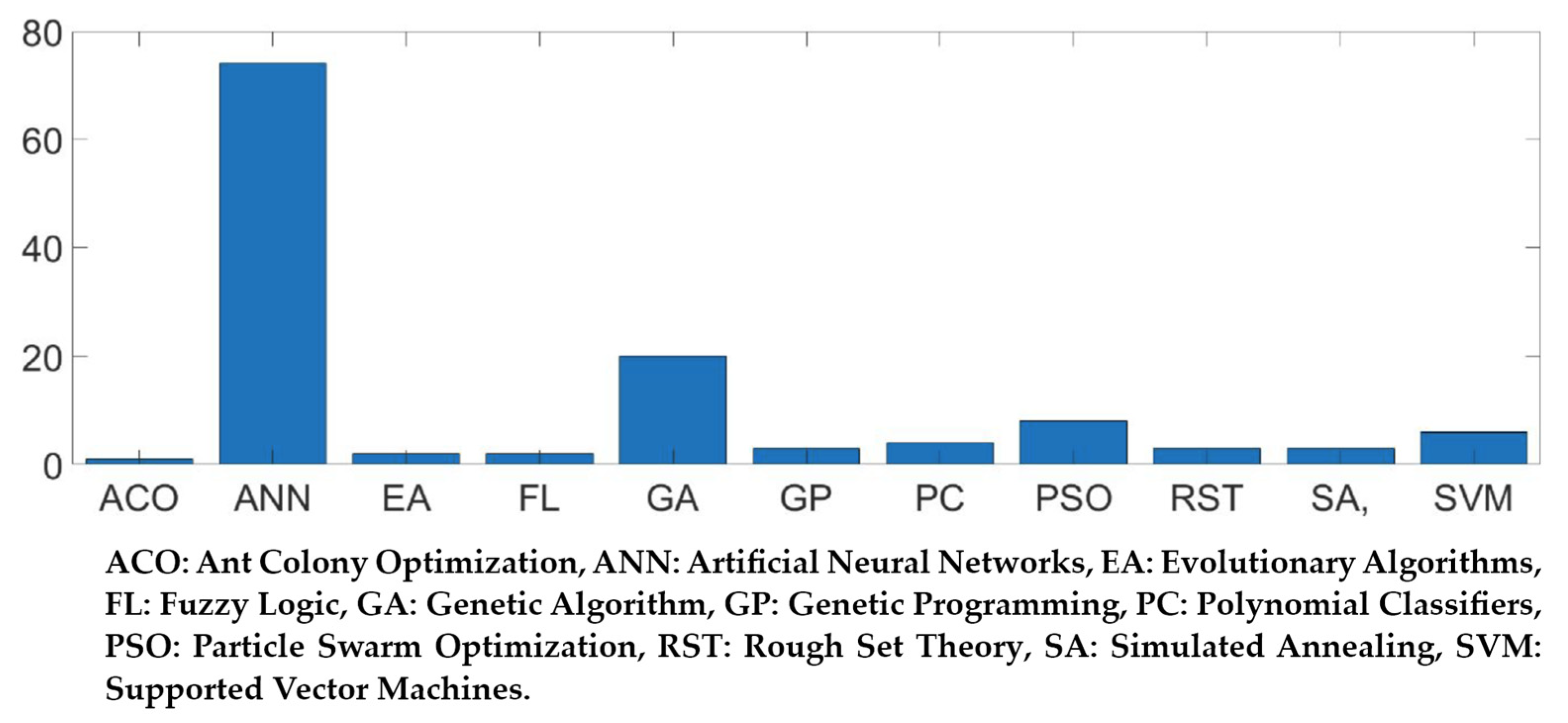
However, as a very complex failure problem that involves the mechanism of fatigue and wear, it is very difficult to establish a satisfactory model to predict FF life accurately [24]. Nowadays, with the rapid development of artificial intelligence, new computational tools like artificial neural networks (ANNs) are widely used for regression problems, classification problems, etc. [25]. These data-driven methods have also matured and been applied in the fatigue field. Depending on the statistics of Ref. [26], ant colony optimization, ANNs, etc., have been used for fatigue life prediction. Among these algorithms, ANN is the most popular one. More than 60% of works have used this method during their research on fatigue cases (as shown in Figure 1). For plain fatigue problems, Dourado and Felipe [27] built a deep neural network (DNN) to predict the corrosion–fatigue damage accumulation, and Yang and Kang [28,29] used a fully connected neural network (FCNN) based on multilayer perceptron (MLP) to predict multiaxial fatigue life. All these models can provide more accurate predictions compared with the traditional methods. The life prediction results given by these data-driven models are generally within ±2 bandwidth for high cycle fatigue cases. However, for fretting fatigue life estimation, just a few works have reported on this. Nowell et al. [30] utilized a multilayer perceptron (MLP) to predict fretting fatigue life, while Oliveira et al. [31,32] employed a multilayer perceptron (MLP) with a training dataset that contained finite element method results for the prediction of fretting fatigue life. These works prove that ANN is a satisfactory method for fretting fatigue life prediction.
Considering that FF is a very complicated multi-factor-influenced problem, it is difficult to establish a complete fretting fatigue evaluation method. Machine learning provides a new way of thinking about solving this problem. Considering that there are few works focused on the application of machine learning on fretting fatigue life prediction, the main work of this paper is to propose a novel methodology for the fretting fatigue life prediction of aluminum alloys, including 2024-T351 and Al4%Cu, based on a neural network (NN) method, called the fretting fatigue life prediction neural network (FFLP-NN). A particle-swarm-optimized back propagation (PSO-BP) algorithm was used to develop the FF model. The training data, such as loading conditions, fatigue life of 2024-T351, and Al4%Cu, were collected from the published literature. To evaluate the accuracy of the model, the prediction results were compared with the SWT criterion.
2. Fretting Fatigue Life Prediction Method
2.1. Critical Plane Approach for Fretting Fatigue Life Prediction
The critical plane (CP) method is developed based on the phenomenological observation of fatigue crack initiation [33]. As the CP approach has an explicit physical meaning and a good correlation with the fretting fatigue (FF) experiment, it is widely used to predict FF life [34]. Among these CP criteria, the SWT [17], which was first applied by Farris and Szowinski [19] in their research, is considered to be the most suitable one for fretting fatigue life prediction.
The SWT criterion was first proposed in 1970, where it was considered as a stress–strain fatigue damage function for metals’ fatigue. In 1987, Socie [35] made some modifications based on experimental data. Since then, the modified criterion has been widely used as a simple and effective method for predicting multiaxial fatigue life. Then, some researchers applied it in FF life prediction and found that it has a better agreement with FF experiments among numerous CP models.
The formula of the modified SWT criterion is as follows:
where σnmax is the maximum normal stress at the critical plane, Δεa/2 is the corresponding strain amplitude on the corresponding surface, σf′ and εf′ are the stress–strain fatigue parameters of the material, and b, c are the experimentally determined parameters. Nf is the fretting fatigue life, and E is Young’s modulus of the material.
The material parameters and experimental parameters of 2024-T351 and Al4%Cu used in the SWT criterion are shown in Table 1.
2.2. Stress and Strain Distribution Analysis
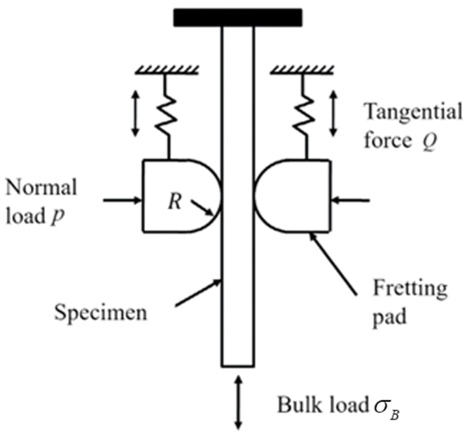
All the fretting fatigue (FF) test data used in this paper are based on typical FF testing, as illustrated in Figure 2. Two cylinder fretting pads are contacted with a plane specimen by normal load P. This structure (fretting pads and specimen) forms a Hertzian contact case whose stress distribution can be described using Hertz contact [36] mechanics. The specimen is fixed on one end and suffers bulk load σB on the other end. The fretting pads are fixed by supporting structures, which can be treated as ‘springs’. With the combined action of load P, σB, and stiffness of the springs, the contact system will generate tangential force Q on the fretting pad. Fretting will happen in the contact region between the specimen and the fretting pad. Fatigue crack will initiate around the contact edge of the specimen after many cycles of σB.
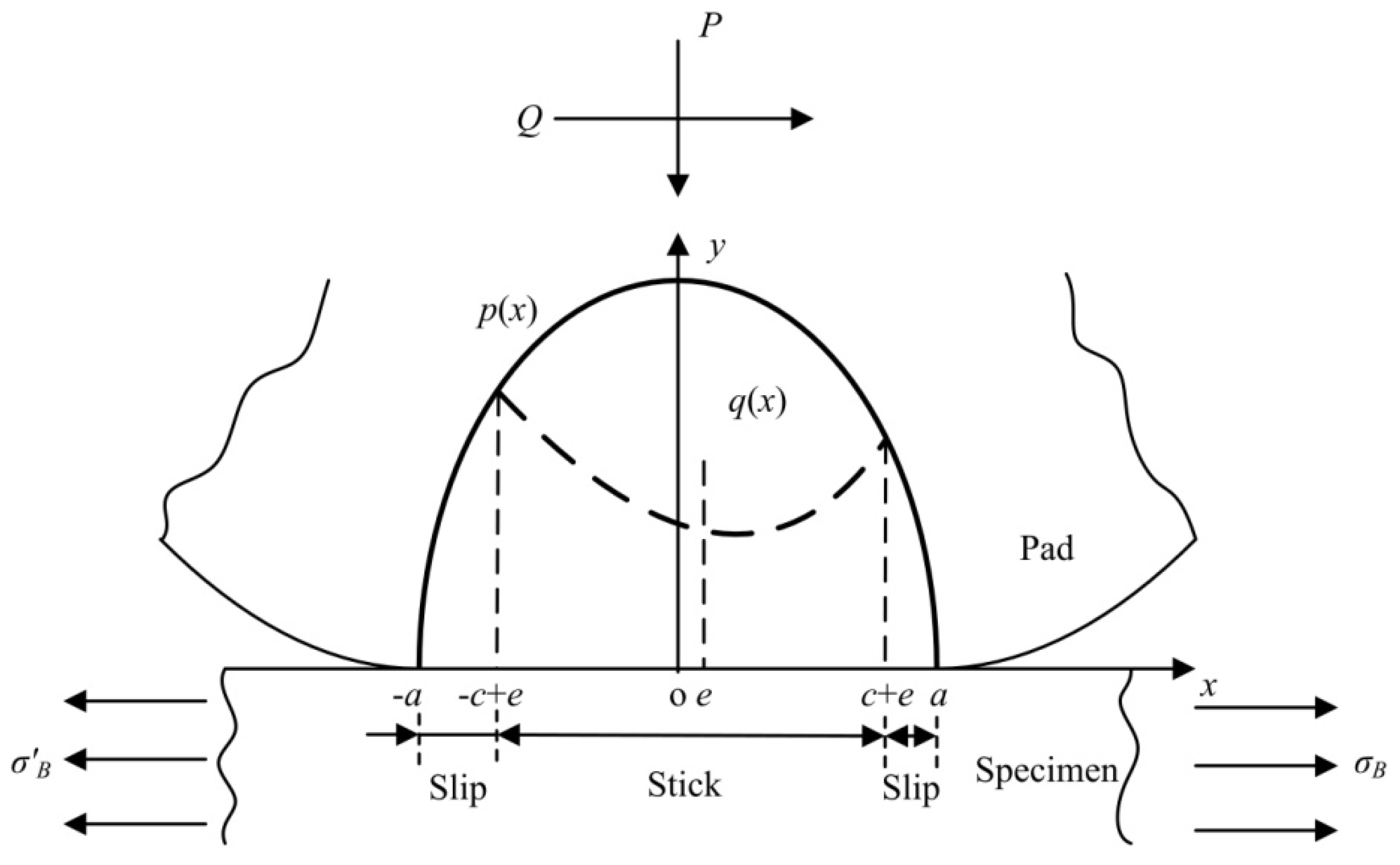
As a non-conforming contact problem, the stress and strain distribution of the contact region directly determined the fatigue behavior of the comportment, as shown in Figure 3, which is also important for the selection of the input factors of the FFLP-NN. This kind of Hertzian contact case was finally solved by Nowell and Hills [37]. As shown in Figure 3, the contact stress destitution is as follows:
where p0 is the max contact pressure, and a is the half width of the Hertz contact [36] region, given by
where P represents the normal load, and E* and R* are the equivalent Young’s modulus and radius of the two contact parts, respectively, given by
where E1, E2 are the Young’s moduli of the two contact parts, respectively, and ν1 and ν2 are the Poisson’s ratios of the two contact parts, respectively.
The shear stress distribution q(x) is [36] as follows:
where q′(x) and q″(x) are given by
where c and e are given by
where μ is the coefficient of friction, and Q is the tangential force.
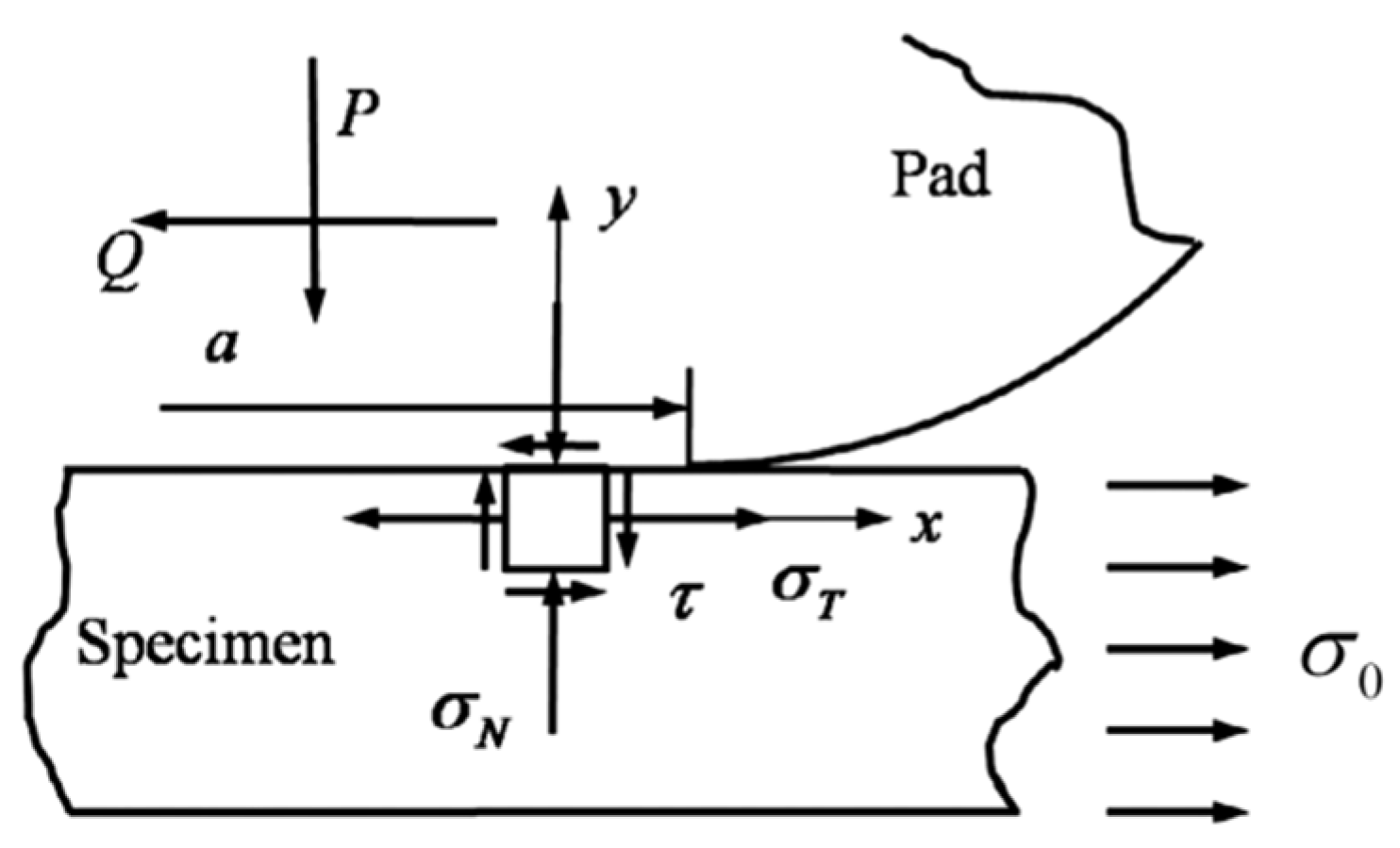
For applying the CP method in FF life prediction, the location and orientation of the critical plane should be determined first. As shown in Figure 4, the contact interface is under a multiaxial stress state. The stress or strain of different contact points in different generic planes can be calculated using the transformation equations, as follows:
where σx, σy, are normal stress and τxy is shear stress on the global coordinate system, εx, εy, are normal strain and γxy is shear strain on the global coordinate system, θ is the orientation of a generic plane, σθ, τθ represent the normal stress and shear stress on a generic plane, respectively, and εθ, γθ present the normal strain and shear strain on a generic plane, respectively.
2.3. Finite Element (FE) Model for Fretting Fatigue
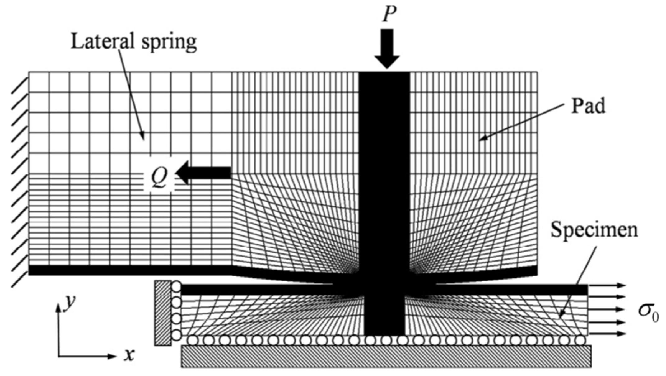
To obtain the stress component illustrated in Figure 5, a finite element (FE) model was established using the commercial FE software ABAQUS (developed by Dassault Systèmes in Paris, France, version Abaqus 2020). As a plane strain problem, a 2D model was used to simplify the numerical calculation.
As shown in Figure 5, the FE model consists of three components: a fretting pad, a lateral spring, and a specimen. The fretting pad was bonded to the lateral spring and put in contact with the specimen. The contact region of the fretting pad and the specimen was meshed by a refined element (element size 10 μm × 10 μm) to agree with the Hertzian analytical solution.
The boundary conditions and constraints applied to the model are shown in Figure 5. In the model, the left part of the lateral spring was set to be fixed. It should be noted that the mission of the lateral spring is to restrain the rigid motion of the fretting pad; thus, a small elastic modulus of the lateral spring is defined. The symmetry boundary was set on the left and lower sides of the specimen to constrain the rigid moment of the specimen. Normal load P is applied on the top edge of the fretting pad, and tangential force Q is applied on the left edge of the fretting pad. Bulk load σB is applied on the right edge of the specimen. A similar model has been used by many studies, and it has been proved to be accurate for fretting fatigue analysis [38].
2.4. Calculation Method of Critical Plane
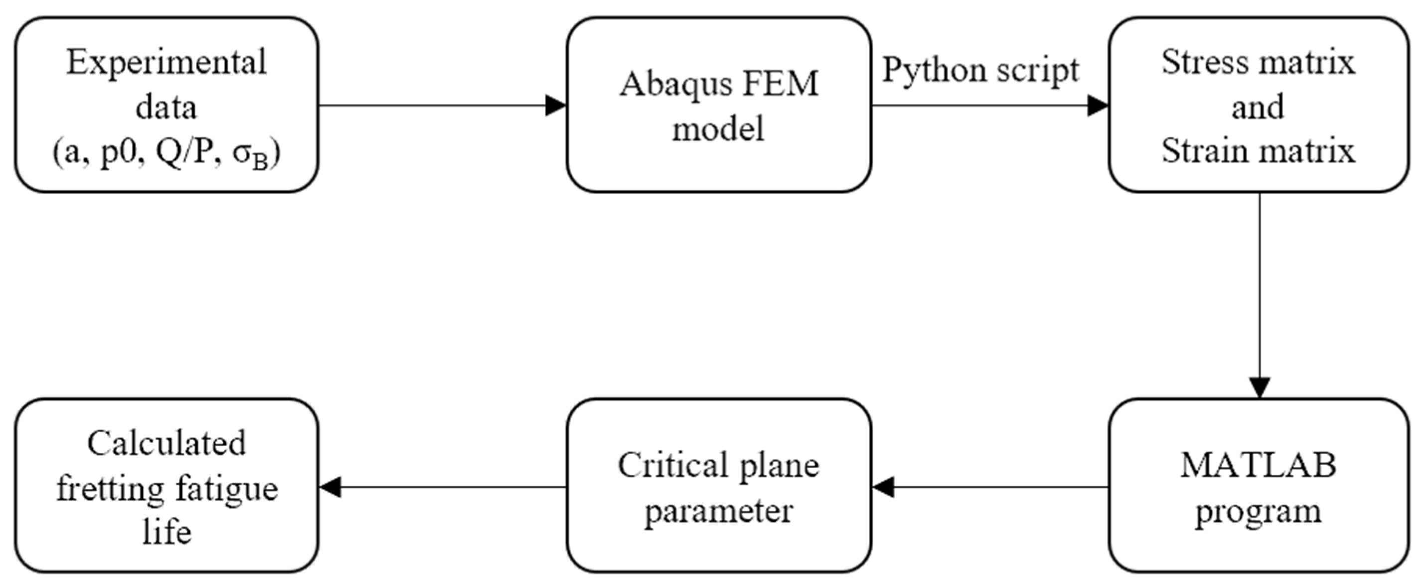
After the calculation was complete, a Python script was employed to retrieve the stress data of each node within the contact area from Abaqus and was saved as a text document in matrix form, with the format of the stress matrix [xi, σxi, σyi, τxyi]. Similarly, the strain data were also saved, with the format of the strain matrix [xi, εxi, εyi, γxyi], where i represents the ith node of the densest area from the specimen’s contact region.
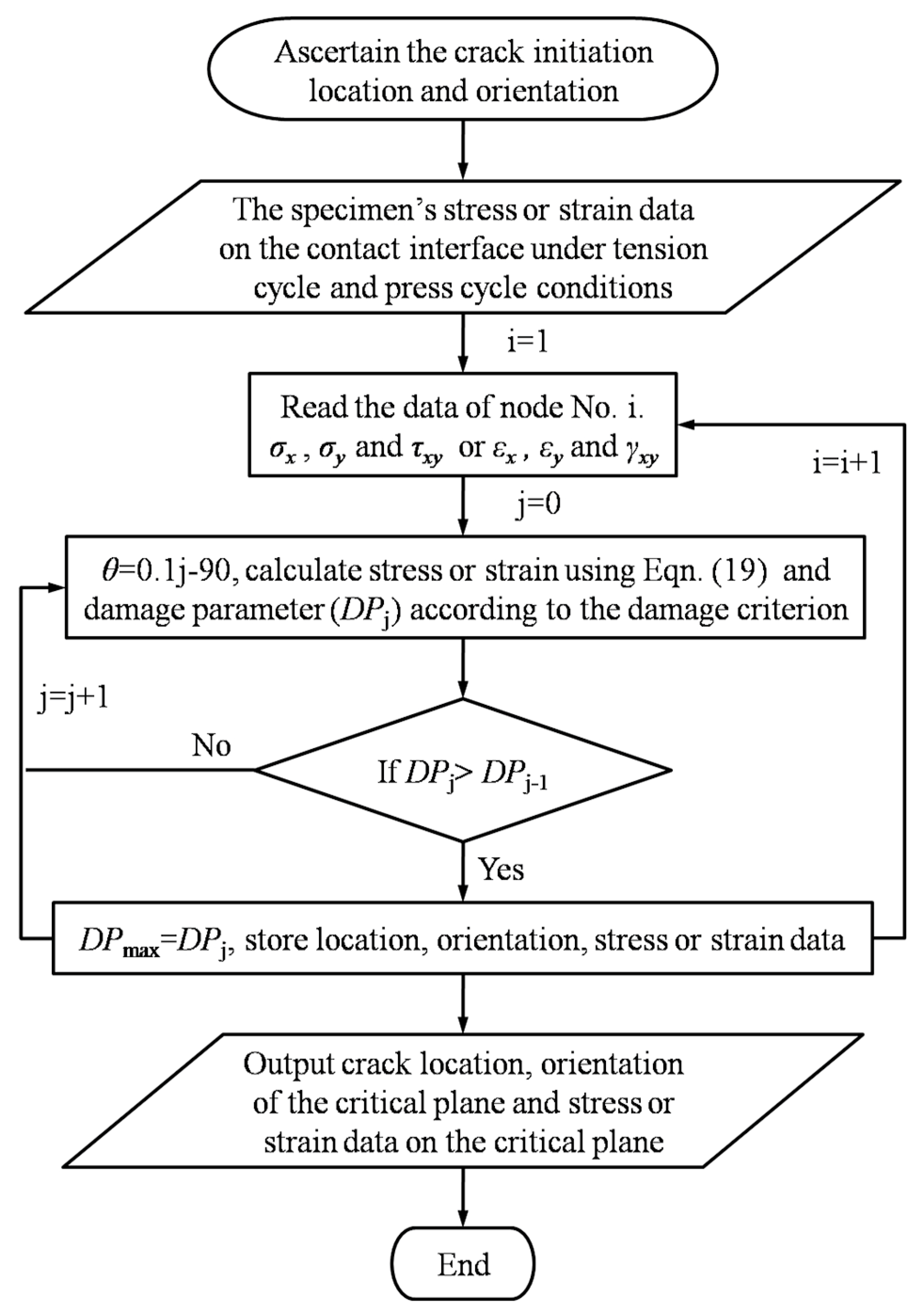
Depending on Equations (12) and (13), a MATLAB code was developed to locate the critical plane. The specimen’s stress or strain data on the contact interface under tension cycle and press cycle conditions were input into the program to calculate the normal stress–strain and shear stress–strain in the critical plane. The flow chart of the program is shown in Figure 6. More details are introduced in Ref. [34].
After all these processes, FF life can be calculated by a certain CP model. The general procedure is illustrated in Figure 7.
3. Artificial Neural Network Architecture
3.1. Multilayer Perceptron
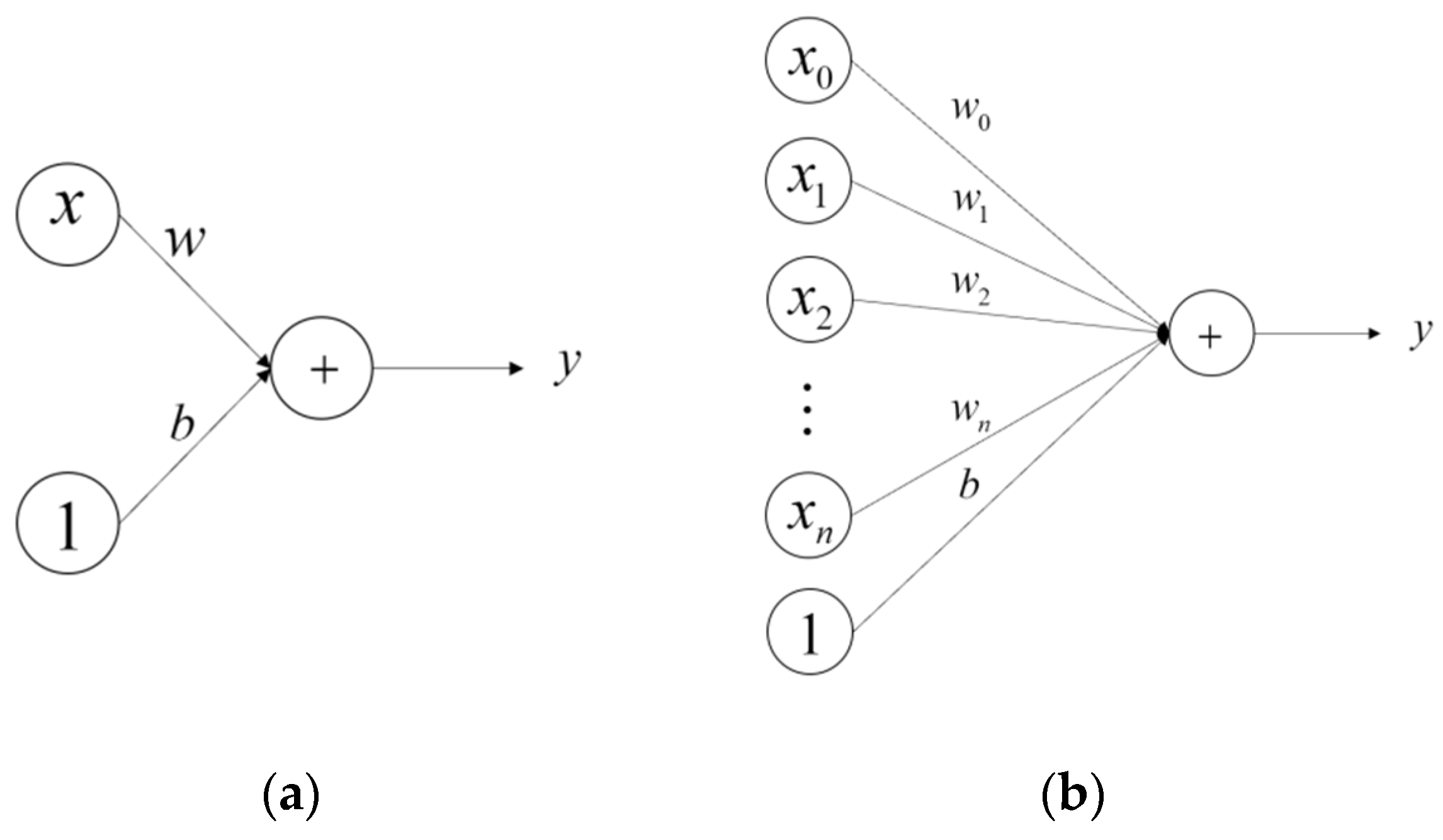
The perceptron [39] is the fundamental unit of classical artificial neural networks and plays a crucial role in neural network algorithms. Figure 8a shows the basic structure of a single perceptron. A single, independent perceptron is capable of performing basic linear regression calculations. When it has one input variable, the perceptron can be represented by the following equation:
where w represents weight, b is the bias, x denotes the input variable, and y represents the output value.
Through iterative calculations, the perceptron autonomously adjusts the weights and biases to minimize the loss between the predicted output value and the true value.
The multilayer perceptron (MLP) [40] is a neural network model that consists of multiple perceptrons and integrates input and output. Figure 8b shows a multiple-input perceptron in MLP. xi represents the ith input variable, and y is the output value. The output of the previous layer serves as the input for the next layer. Meanwhile, multiple input, which is presented as a matrix, is also allowed. Then, Equation (14) changes to the following:
Depending on this feature and structure, MLP can be used to deal with multi-factor-influenced nonlinear problems, such as FF life prediction.
3.2. Particle-Swarm-Optimized Back Propagation (PSO-BP) Neural Network
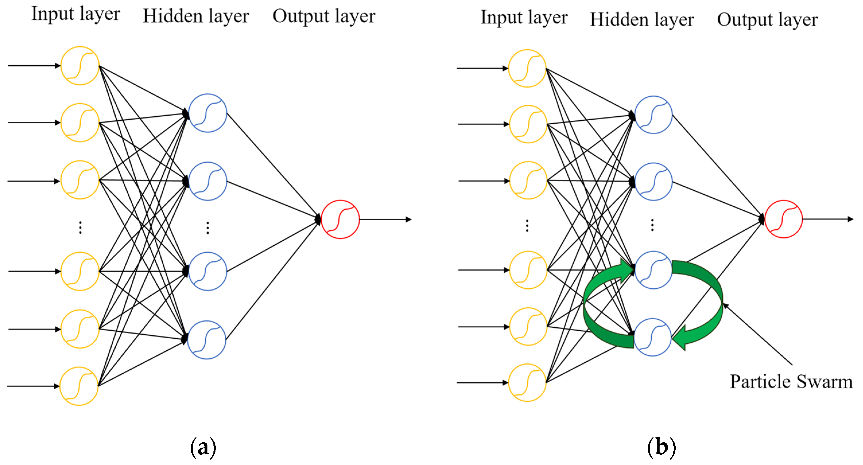
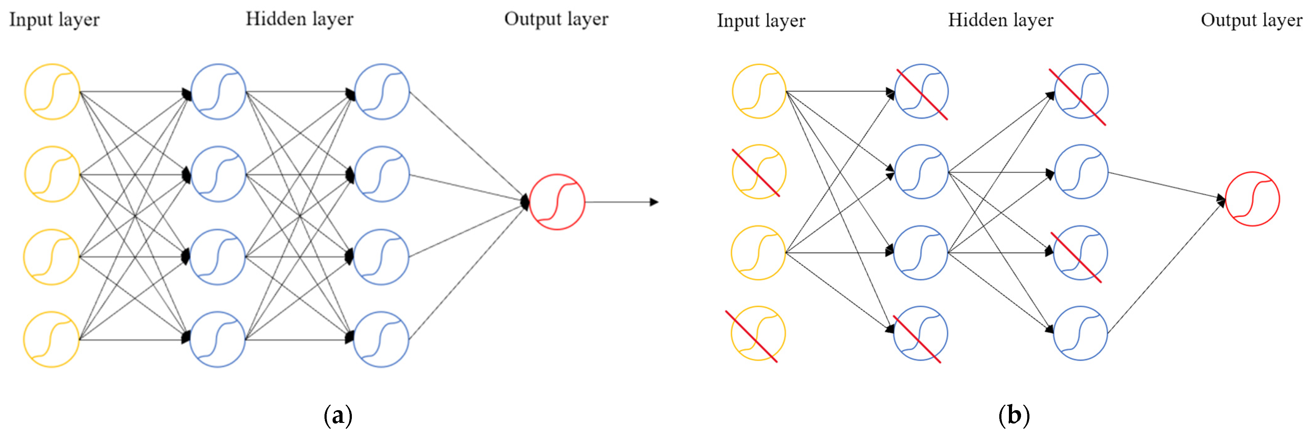
The particle swarm optimization (PSO) algorithm [41] is a path-planning algorithm designed for local path optimization. In the backpropagation (BP) neural network [39], each perceptron in every layer possesses distinct weights and biases. However, not all of this information is adjusted to reduce error. The PSO algorithm introduces the concept of particle swarm optimization into each layer, aiming to trace the local optimal perceptron through optimization [42]. By employing the PSO algorithm, the learning rate and fitting effect of the BP neural network can be effectively enhanced. Compared to the original BP neural network, the PSO-BP combination achieves faster convergence speed and improved prediction accuracy under the same scale of training samples. The architecture diagrams for both BP and PSO-BP are illustrated in Figure 9.
4. The Development of the Fretting Fatigue Life Prediction Neural Network (FFLP-NN)
4.1. Data Selection and Pre-Processing
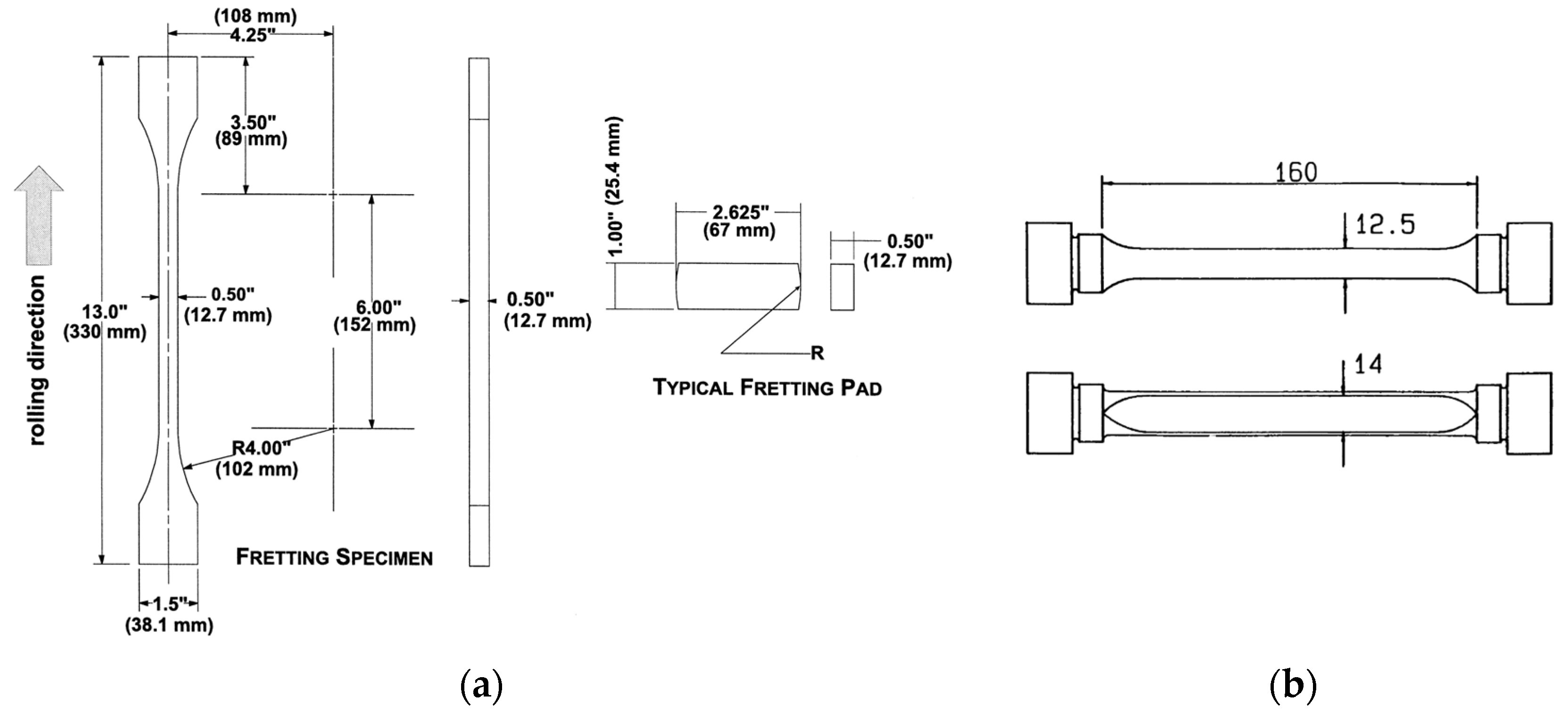
The fretting fatigue experimental data of aluminum alloy collected for the model were obtained from Nowell’s experiment data of Al4%Cu [43] and Farris and Szolwinski’s experiment data of 2024-T351 [19]; all the collected data are shown in Table 2 and Table 3. The shape and size of Farris and Nowell’s specimens are shown in Figure 10.
The choice of the input parameters is a key step for the training of the FFLP-NN. To highlight the character of FF, three types of parameters were picked: (1) normal load p0 and bulk load σB, which reflect the loading condition; (2) half-width a, which reflects the contact geometry; and (3) stress ratio Q/P, which reflects the wear behavior. Some of these parameters were also used by Nowell et al. [30] and were proved to be efficient for ANN model training.
Generally, fretting fatigue is treated as a high-cycle fatigue phenomenon whose fatigue life usually ranges from 105 to 107 cycles [44]. Depending on the concept of the fatigue limit, experiment fretting fatigue cycles over 107 are all treated as run-outs. The run-out data will introduce training noise. So, all the run-out data were removed from the dataset. According to Table 2 and Table 3, the target variable Nf (fretting fatigue life) is much larger than any of the input variables. It is recommended that the target variable should have the same order of magnitude as the input variables. So, the target variable Nf was processed following these rules before training:
All the data were divided into three parts, including a training set, a test set, and a validation set. Considering that the total non-duplicate data only contain 56 groups, about 10% of the data, a total of 6 groups were chosen randomly and separately as validation data. The residual 90% groups form the training set.
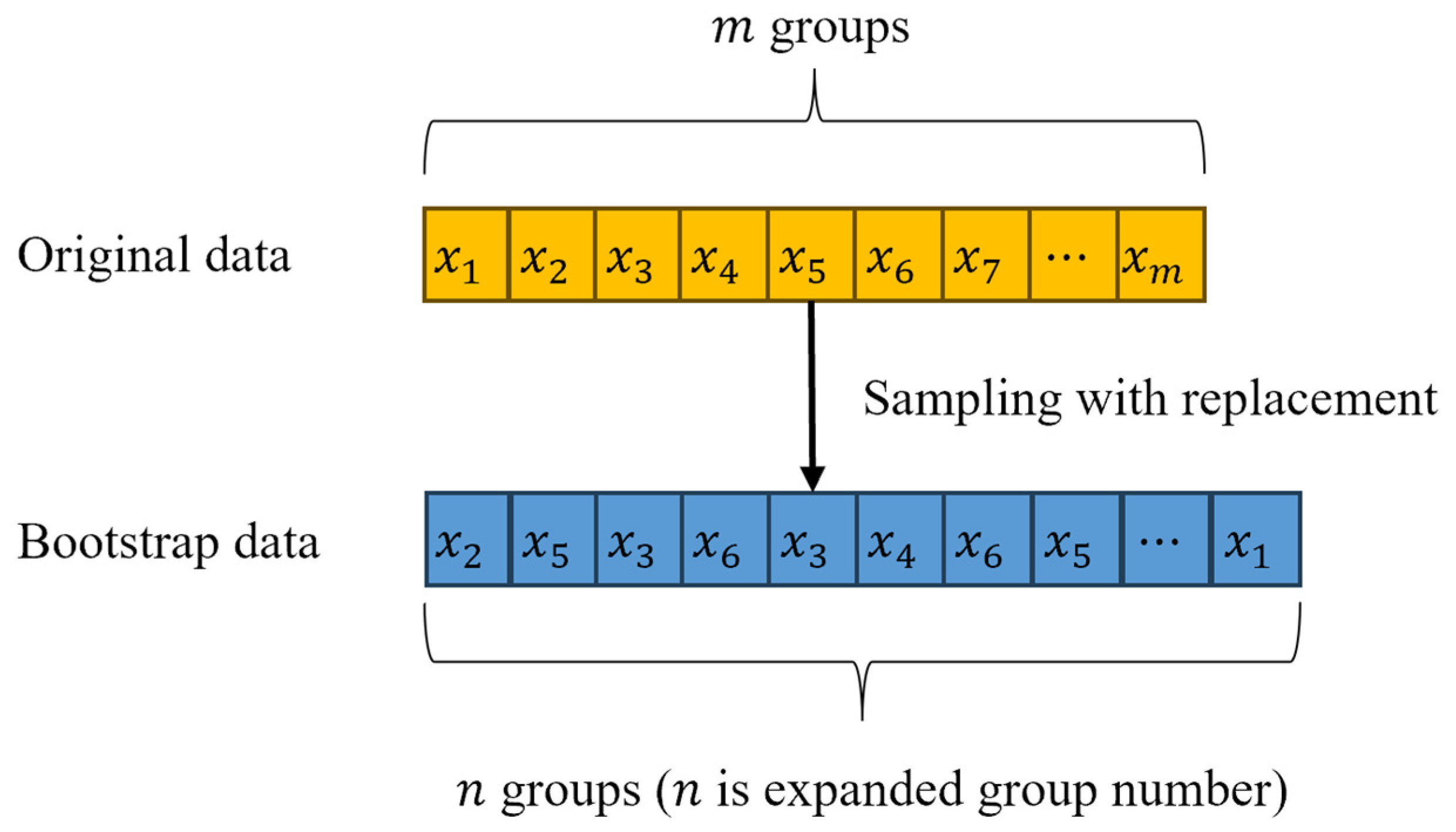
The quantity of the available experiment data is limited, which is insufficient for model training. To solve this small sample problem, expanding the dataset is necessary. In statistics, to enhance the observation of the distribution characteristics of a small amount of data, a sample expansion method called bootstrap [45] is generally used. This method is essentially a subsequent sampling with a return. The principle is as follows:
where Xi′ represents the ith sample in the expanded dataset, and Xj represents the randomly selected j th sample value from the original dataset. The bootstrap process is shown in Figure 11.
Then, the training set used in this training is extended to a dataset containing a total of 500 sets of data after 10 times of bootstrap expansion.
The test set is used to self-evaluate the training results during the training process. It is randomly selected from the training set. To clearly and objectively represent the training results, the scale of the test set should not be too large. In this process, it is limited to 10% of the training set [46].
Considering that the input variables are quite different in magnitude order, all the input data need to be normalized before the training process. Otherwise, incorrect amplification will occur or there will be a reduction in the impact of certain factors by unsuitable local weights, thereby influencing the accuracy of the NN model. In this paper, the MinMax normalization method (Equation (18)) [47] was employed. This normalization technique scales the values of the input variables to a specific range (typically between 0 and 1) based on the minimum and maximum values observed in the dataset using the following equation:
where Xnorm, X, Xmax, Xmin are the normalized, original, maximum, and minimum values of parameter X, respectively.
4.2. Parameters Setting for PSO-BP Neural Network
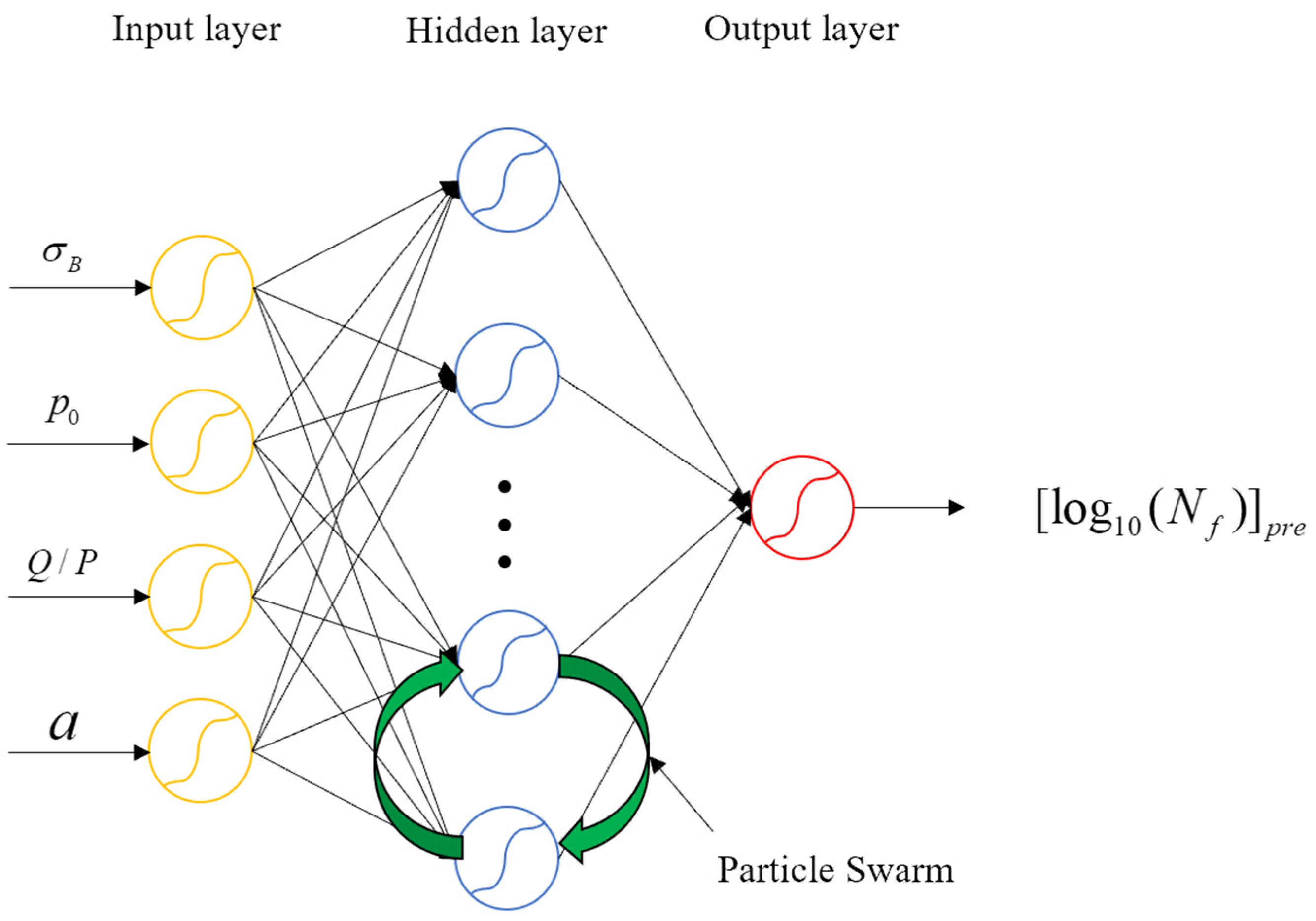
The exact structure of the FFLP-NN based on the PSO-BP algorithm is shown in Figure 12. The FFLP-NN has one input layer, one hidden layer, and one output layer. The input layer has four units; the hidden layer has eight units; and the output layer has one unit represented as a single output. The activation function between the input layer and the hidden layer is ReLU [48], which is a function that is widely used in prediction works. The rule of ReLU is as follows:
Considering that the output value of the hidden layer will also be treated as the input value of the output layer, the calculation of the hidden layer may contain a negative value, and ReLU can only retain the non-negative character of the input value. So, the activation function between the hidden layer and output layer is Leaky_ReLU, which can retain the negative character of the input value. The rule of Leaky_ReLU is as follows:
A dropout stage [49] (shown in Figure 13) and an L2 regulation method were set after the calculation of each layer (except the output layer) to prevent overfitting during training. The dropout ratio of each layer is set to be 50%, and the L2 regulation value is 0.2. The initializer function of the input data is ‘He-normal’, which is suitable for the ReLU activation function.
The learning rate can affect the convergence speed and learning effect of the model. The appropriate setting can achieve optimal results of both the learning effect and convergence speed. An adaptive moment estimation (Adam) optimizer [50], which can automatically adjust the learning rate according to the model’s convergence effect, was utilized to optimize the learning rate. The loss function of this model in terms of the mean square error is as follows:
where [log10(Nf)]pre represents the output prediction result of the model.
After trial training and optimization, the batch size (a hyper-parameter that defines the volume of samples in one training iteration) was set to 32, which was recommended in the NVIDIA® CUDA® (Compute Unified Device Architecture) developer’s guide; the number of epochs (a hyper-parameter which defines the times of training iteration) was set to be 100, which makes the training loss stably close to 0, and no overfit happened.
As a small sample case, to ensure the training effect of the model, a cross-validation method [51] was adopted during training. The particle swarm setting includes four particle swarm sizes with a maximum of 10 iterations. The concrete number of cross-validation times is three. All the hyper-parameters were adjusted manually; the main aim of this adjustment was to find suitable parameters which could achieve high training accuracy and prevent overfitting. After many turns of adjusting, the main hyper-parameters were determined, and they are outlined in Table 4. The model training was completed by NVIDIA® GeForce RTXTM 3070, and the model was built based on TensorFlow 2.6.
4.3. The Training Process of the Fretting Fatigue Life Prediction Neural Network (FFLP-NN) Model
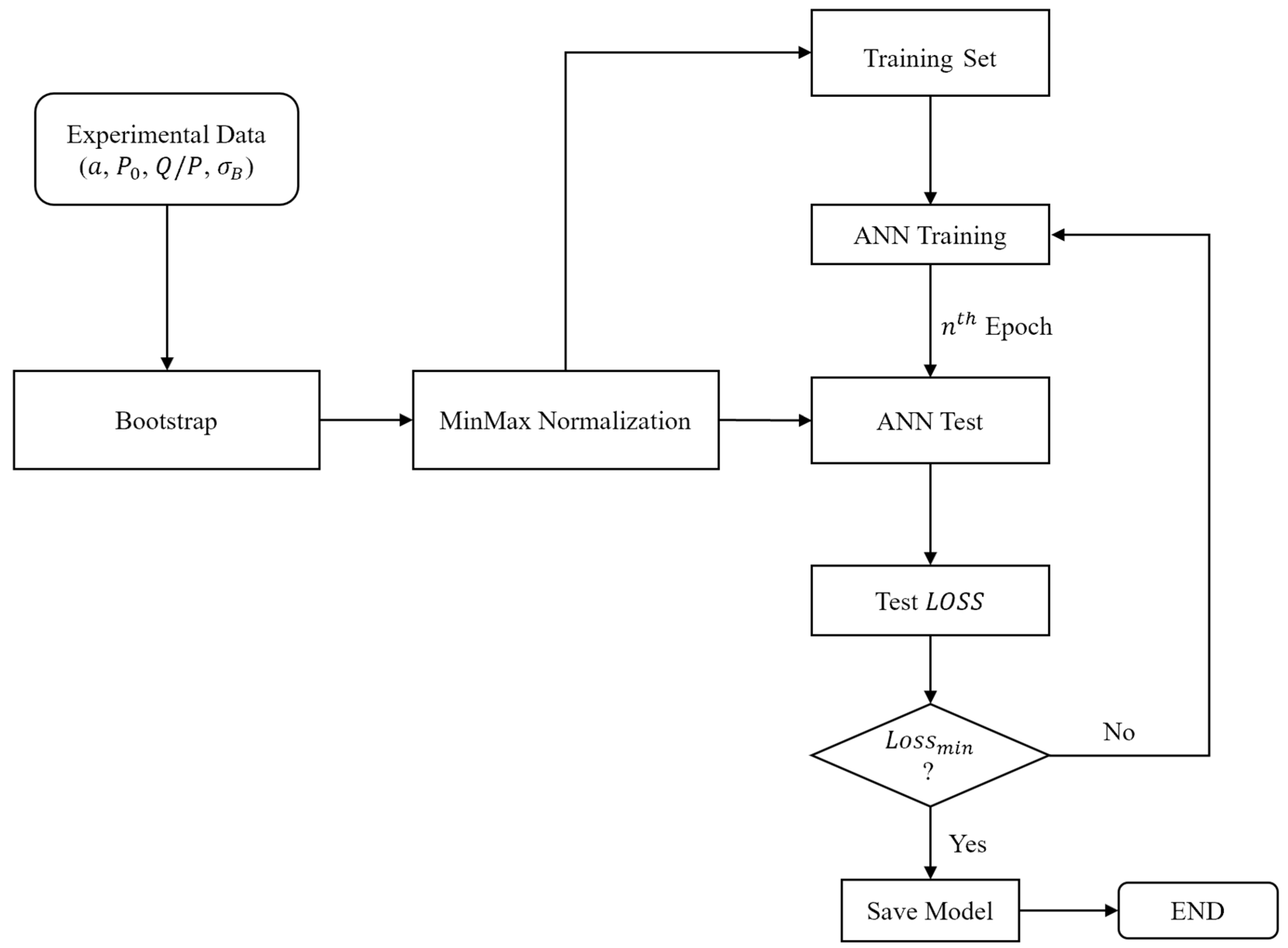
To sum up, the training process is shown in Figure 14. Firstly, the input parameters are collected from the experiment data, and a bootstrap algorithm is used to expand the sample set. The normalization method is used to edit the origin data and form the input matrix. The expanded sample set is divided into training sets, test sets, and validation sets by random sampling. Secondly, the training and test sets are inputted into the PSO-BP neural network. The best value of weights is captured by minimizing the test loss. Finally, training is stopped, and the model is saved.
5. Results and Discussion
5.1. The Prediction Results on Training Set of the FFLP-NN Model
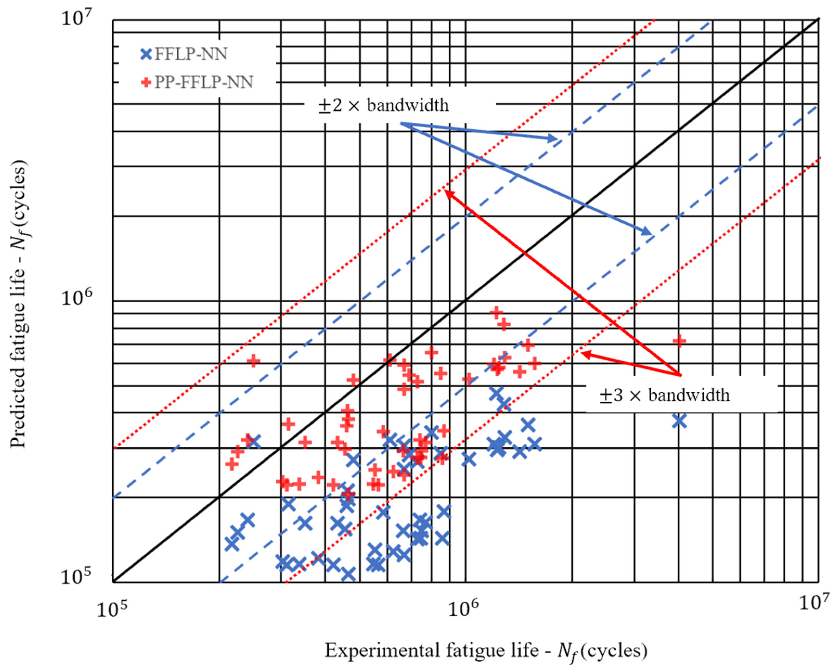
To further examine the training results of the model, the prediction life vs. experiment life of the training set is shown in Figure 15. Obviously, the distribution of the FFLP-NN data points in the figure is consistent with the diagonal (black solid line, which means that the prediction result is the same as the experiment result), but the overall prediction result is small. Nearly half of the data points fall below the ±3 bandwidth (red dotted line). This means that the FFLP-NN model can provide fretting fatigue life prediction regularly, but it usually provides conservative results.
Because this is a small sample training case, the prediction results given by the trained model always include a small error compared with the real value. Thus, post-processing [52] is a common method used for compensating for this error to improve the prediction accuracy, such as the weather forecasting area [53]. The simplest post-processing method is to add an error to the prediction result, as shown in Equation (22). Therefore, the prediction results are all translated at a distance, and more accurate prediction results can be obtained.
where Npre′ presents the post-processed prediction result, and Etra is the error obtained by calculating the prediction mean square error on the training set (Equation (23)). It should be stated that the value of Etra is constant after the training process. All the predictions of the trained model will use the same value of Etra. The post-processing fretting fatigue life prediction neural network (PP-FFLP-NN) prediction results on the training set are also given in Figure 14. It can be seen that PP-FFLP-NN’s performance is much better than the FFLP-NN. Almost all the prediction results are within the ±3 bandwidth, over 50% of the prediction results are within the ±2 band (blue dashed line), and only two prediction results fall outside the ±3 bandwidth. Considering that there are only 50 groups of experiment data available for the training of the model, the performance of the model is satisfactory.
5.2. Comparative Analysis
5.2.1. Evaluate Parameters
- (1)
- Average accuracy rate
Due to the potential deviations in the prediction results, the conventional calculation of the average relative error [54] formula may magnify the errors in the prediction results, which are larger than those in the experiment results. To overcome this issue, a new calculation formula called the ‘average accuracy rate’ was designed to evaluate the prediction performance. The formula for calculating the average accuracy rate is as follows, and the calculation result of the average accuracy rate will be expressed in percentage form:
where i presents the ith group of the data. If the average accuracy rate is lower than 100%, this indicates that the prediction results tend to be shorter than the true values on average, suggesting a conservative prediction. Conversely, if the average accuracy rate is higher than 100%, this means that the prediction results tend to be larger than the true values on average, indicating a radical prediction. A 100% average accuracy rate implies that the prediction results are the same as the true values on average, indicating a completely accurate prediction.
- (2)
- Floating range
Considering the generalization ability of this model, we generated extra experiment data (to ensure that the model is completely unfamiliar with the data). The prediction results of the extra experiment can effectively verify the generalization ability of the SWT, FFLP-NN, and PP-FFLP-NN.
Considering that the generalization ability of this model is hard to describe, a new calculation formula called ‘floating range’ was designed to evaluate the generalization ability. It was noticed that the value of a floating range close to 0 means better generalization ability. The floating range is defined as follows:
where AccVal presents the average accuracy rate in the validation set, and AccExp presents the average accuracy rate in the extra experiment data.
5.2.2. Prediction Results of the Validation Set and Extra Experiment Data
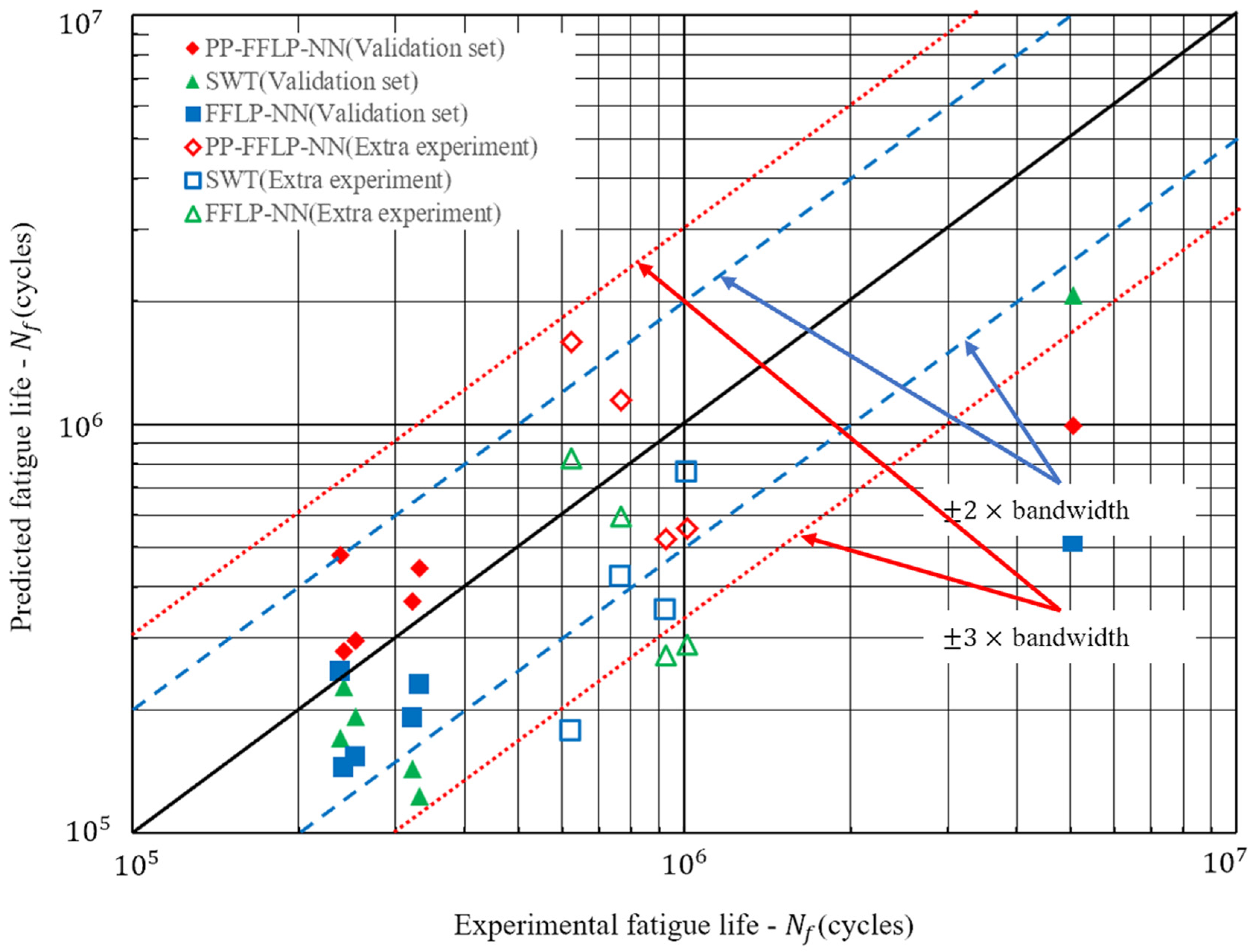
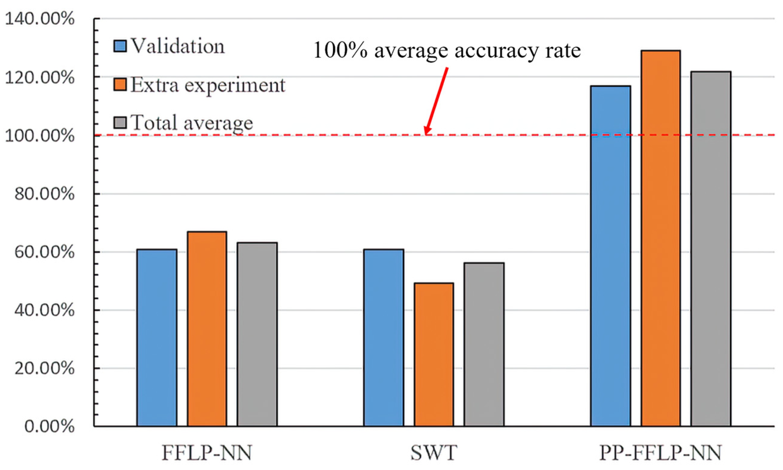
The validation dataset is extracted independently from the training data before model training, which is unfamiliar data for the model. In addition, our research group conducted four groups of extra experiments (Table 5) to verify the prediction performance and generalization ability of the model. All the prediction results on the validation set and the extra experiment data are shown in Figure 16. The average accuracy rate of each model is shown in Table 6 and Figure 17. The floating range of each model is shown in Table 7.
Figure 15 shows that, for the validation set, over 80% of the prediction results given by the FFLP-NN fall within the ±2 bandwidth (blue dashed line), while just 50% of the SWT prediction results fall within the ±2 bandwidth, and the rest fall within the ±3 bandwidth (red dotted line). The prediction results of the PP-FFLP-NN are closer to the true life compared with FFLP-NN results. The average accuracy of the SWT, FFLP-NN, and PP-FFLP-NN are 60.82%, 60.74%, and 116.99%. This reflects that the accuracy of the SWT and FFLP-NN is almost the same; the PP-FFLP-NN’s prediction accuracy is the best. In the extra experiment evaluation, 75% of the prediction results of the PP-FFLP-NN fall within the ±2 bandwidth, and all the results fall within the ±3 bandwidth. The FFLP-NN and SWT do not perform as well as the PP-FFLP-NN. The PP-FFLP-NN reached an average accuracy rate of about 129.03%, and the SWT and FFLP-NN only obtained rates of 49.24% and 66.98%. This shows that after the post-processing stage, the model’s performance is better than the SWT and FFLP-NN, and not only in the training and validation set; the PP-FFLP-NN can provide accurate prediction results even when faced with completely unfamiliar input data.
As shown in Table 6, for the generalization ability evaluation, the FFLP-NN and PP-FFLP-NN have the same floating range at about 9.88%; the SWT model is at 20.59%. This means that the applicability of the SWT model is not as good as the FFLP-NN and PP-FFLP-NN for large-range FF life prediction.
Considering the prediction accuracy, the above discussion shows that the FFLP-NN and PP-FFLP-NN can give more accurate predictions than the critical plane method. The traditional phenomenological or physical-related FF life prediction models usually just consider the stress or strain in the contact region to propose FF damage. On the one hand, most of these models or criteria are referenced from other fatigue cases, such as multiaxial fatigue cases. They do not consider fretting-related parameters to reflect the particularity of FF. On the other hand, fretting is a very complex phenomenon that cannot fully consider the main influence factors to establish a complete damage model, while NN is good at modeling multi-factor incomplete mechanism problems. However, depending on the validation set test, there was a prediction point (as shown in Figure 16) that only the SWT prediction fell within ±3 bandwidth; both the FFLP-NN and PP-FFLP-NN lost their accuracy. This is probably because there is only one training sample near the FF life of 5 × 10⁶ cycles. For data-driven neural networks, when the training samples cover less or no data, the prediction results tend to become unreliable; the traditional critical plane method based on a physical model will maintain its accuracy. Therefore, integrating physical information may improve the prediction accuracy of neural networks in this situation; further research is needed to verify this point. Even so, NN is still a powerful method for FF life prediction.
Considering the predicting efficiency, traditional FF life prediction based on the CP method always has the following steps: confirm loading data and material; carry out finite element (FE) calculation; find critical plane parameters; and calculate fatigue life. Finishing all the steps will take a lot of time and resources, but a trained ANN will provide the prediction result directly. The advantage of ANNs in life predicting efficiency is huge, and ANNs are based on statistics methodology, meaning that the prediction accuracy will increase after introducing more experimental data into training.
6. Conclusions and Future Prospects
In this paper, an FFLP-NN based on the PSO-BP neural network was trained for the fretting fatigue life prediction of aluminum alloys, including 2024-T351 and Al4%Cu. The input variables contain bulk load σB, loading ratio Q/P, the half-width of the Hertz contact area a, and maximum normal load p0. The output target variable was logarithmic processed fretting fatigue life data. We added a post-processing stage to the model to obtain better accuracy performance. According to the test result and evaluating indicators, the main conclusions of this paper are as follows:
- (1)
- The FFLP-NN based on the PSO-BP algorithm shows its good performance in small sample problems. Even though the training set only contains 50 groups of non-duplicate data, the FFLP-NN can also provide reasonable prediction results. However, the FFLP-NN without post-processing usually gives conservative predictions. This shows that post-processing can improve the model’s prediction accuracy.
- (2)
- In the validation test, the prediction results given by the FFLP-NN and PP-FFLP-NN are closer to the experiment results compared with the SWT prediction results. The PP-FFLP-NN model performs the best among the three models.
- (3)
- In the extra experiment test, three-quarters of the PP-FFLP-NN results fall within the ±2 bandwidth, and all the results fall within the ±3 bandwidth. The FFLP-NN and SWT did not perform as well as the PP-FFLP-NN. The performance of the PP-FFLP-NN is much better than the FFLP-NN and SWT. This shows that the post-processing stage can not only prove the prediction accuracy in the training and validation set but can also improve the accuracy even when faced with completely unfamiliar input data.
- (4)
- For the generalization ability of each model, the FFLP-NN and PP-FFLP-NN have the same floating range. The SWT model cannot give as accurate prediction results as the FFLP-NN and PP-FFLP-NN for large-range FF life prediction.
Taking all these conclusions into account, here are the prospects:
- (1)
- The ANN technique is based on statistics methodology; the prediction accuracy will increase after adding more experiment data into training and updating the model in future investigations.
- (2)
- The post-processing technique shows the optimistic effect on the ANN model prediction accuracy, and the CP method has physical meanings. Trying to integrate the CP method as a post-processing rule into ANNs may enhance the reliability of the ANN model.
Author Contributions
Conceptualization, X.L. and J.Y.; Methodology, X.L. and H.Y.; software, H.Y.; Validation, X.L. and H.Y.; Formal analysis, X.L. and J.Y.; Investigation, J.Y.; Resources, J.Y.; Data curation, X.L. and H.Y.; Writing—original draft preparation, H.Y.; Writing—review and editing, X.L.; Visualization, X.L. and H.Y.; supervision, J.Y.; Project administration, X.L. and J.Y.; Funding acquisition, X.L. and J.Y. All authors have read and agreed to the published version of the manuscript.
Funding
This research was funded by Science and Technology Plan Project of State Administration for Market Regulation of China Project 2021MK176. And The APC was funded by Beijing University of Civil Engineering and Architecture.
Data Availability Statement
The original contributions presented in the study are included in the article, further inquiries can be directed to the corresponding author.
Acknowledgments
Xin Liu from the Key Laboratory of Special Equipment Safety and Energy-saving for State Market Regulation, China Special Equipment Inspection and Research Institute (CSEI) is gratefully acknowledged.
Conflicts of Interest
The authors declare no conflict of interest.
References
- Waterhouse, R.B. Fretting Fatigue. Int. Mater. Rev. 1992, 37, 77–98. [Google Scholar] [CrossRef]
- Araújo, J. The Effect of Rapidly Varying Contact Stress Fields on Fretting Fatigue. Int. J. Fatigue 2002, 24, 763–775. [Google Scholar] [CrossRef]
- Croccolo, D.; De Agostinis, M.; Fini, S.; Olmi, G.; Robusto, F.; Scapecchi, C. Fretting Fatigue in Mechanical Joints: A Literature Review. Lubricants 2022, 10, 53. [Google Scholar] [CrossRef]
- Beard, J. An Investigation into the Mechanisms of Fretting Fatigue. Ph.D. Thesis, University of Salford, Salford, UK, 1982. Available online: http://ethos.bl.uk/OrderDetails.do?uin=uk.bl.ethos.237768 (accessed on 18 February 2024).
- Waterhouse, R.B. Fretting Corrosion. Proc. Inst. Mech. Eng. 1955, 169, 1157–1172. [Google Scholar] [CrossRef]
- Ruiz, C.; Boddington, P.H.B.; Chen, K.C. An Investigation of Fatigue and Fretting in a Dovetail Joint. Exp. Mech. 1984, 24, 208–217. [Google Scholar] [CrossRef]
- Jin, O.; Mall, S. Effects of Slip on Fretting Behavior: Experiments and Analyses. Wear 2004, 256, 671–684. [Google Scholar] [CrossRef]
- Nix, K.J.; Lindley, T.C. The Influence of Relative Slip Range and Contact Material on the Fretting Fatigue Properties of 3.5NiCrMoV Rotor Steel. Wear 1988, 125, 147–162. [Google Scholar] [CrossRef]
- Madge, J.J.; Leen, S.B.; Shipway, P.H. The Critical Role of Fretting Wear in the Analysis of Fretting Fatigue. Wear 2007, 263, 542–551. [Google Scholar] [CrossRef]
- Findley, W.N. A Theory for the Effect of Mean Stress on Fatigue of Metals Under Combined Torsion and Axial Load or Bending. J. Eng. Ind. 1959, 81, 301–305. [Google Scholar] [CrossRef]
- McDiarmid, D.L. A General Criterion for High Cycle Multiaxial Fatigue Failure. Fatigue Fract. Eng. Mater. Struct. 1991, 14, 429–453. [Google Scholar] [CrossRef]
- Matake, T. An Explanation on Fatigue Limit under Combined Stress. Bull. JSME 1977, 20, 257–263. [Google Scholar] [CrossRef]
- Fash, J.; Socie, D.; McDowell, D. Fatigue Life Estimates for a Simple Notched Component Under Biaxial Loading. In Multiaxial Fatigue; ASTM International: West Conshohocken, PA, USA, 1985; pp. 497–513. [Google Scholar] [CrossRef]
- Lohr, R.D.; Ellison, E.G. A Simple Theory for Low Cycle Multiaxial Fatigue. Fatigue Fract. Eng. Mater. Struct. 1980, 3, 1–17. [Google Scholar] [CrossRef]
- Kanazawa, K.; Miller, K.J.; Brown, M.W. Low-Cycle Fatigue Under Out-of-Phase Loading Conditions. J. Eng. Mater. Technol. 1977, 99, 222–228. [Google Scholar] [CrossRef]
- Fatemi, A.; Socie, D.F. A Critical Plane Approach to Multiaxial Fatigue Damage Including Out-Of-Phase Loading. Fatigue Fract. Eng. Mater. Struct. 1988, 11, 149–165. [Google Scholar] [CrossRef]
- Li, J.; Zhang, Z.; Sun, Q.; Li, C.; Qiao, Y. A New Multiaxial Fatigue Damage Model for Various Metallic Materials under the Combination of Tension and Torsion Loadings. Int. J. Fatigue 2009, 31, 776–781. [Google Scholar] [CrossRef]
- Smith, K.N.; Watson, P.; Topper, T.H. A stress-strain function for the fatigue of metals. J. Mater. JMLSA 1970, 5, 767–778. [Google Scholar]
- Szolwinski, M.P.; Farris, T.N. Observation, Analysis and Prediction of Fretting Fatigue in 2024-T351 Aluminum Alloy. Wear 1998, 221, 24–36. [Google Scholar] [CrossRef]
- Hwang, D.H.; Cho, S.-S. Fretting Fatigue Life Estimation Using Fatigue Damage Gradient Correction Factor in Various Contact Configurations. J. Mech. Sci. Technol. 2017, 31, 1127–1134. [Google Scholar] [CrossRef]
- Ding, J.; Houghton, D.; Williams, E.J.; Leen, S.B. Simple Parameters to Predict Effect of Surface Damage on Fretting Fatigue. Int. J. Fatigue 2011, 33, 332–342. [Google Scholar] [CrossRef]
- Navarro, C.; Munoz, S.; Dominguez, J. On the Use of Multiaxial Fatigue Criteria for Fretting Fatigue Life Assessment. Int. J. Fatigue 2008, 30, 32–44. [Google Scholar] [CrossRef]
- Ding, J.; Sum, W.S.; Sabesan, R.; Leen, S.B.; McColl, I.R.; Williams, E.J. Fretting Fatigue Predictions in a Complex Coupling. Int. J. Fatigue 2007, 29, 1229–1244. [Google Scholar] [CrossRef]
- Wang, J.; Zhou, C. Analysis of Crack Initiation Location and Its Influencing Factors of Fretting Fatigue in Aluminum Alloy Components. Chin. J. Aeronaut. 2022, 35, 420–436. [Google Scholar] [CrossRef]
- Montesinos López, O.A.; Montesinos López, A.; Crossa, J. Fundamentals of Artificial Neural Networks and Deep Learning. In Multivariate Statistical Machine Learning Methods for Genomic Prediction; Springer International Publishing: Cham, Switzerland, 2022; pp. 379–425. [Google Scholar] [CrossRef]
- Kalayci, C.B.; Karagoz, S.; Karakas, Ö. Soft Computing Methods for Fatigue Life Estimation: A Review of the Current State and Future Trends. Fatigue Fract. Eng. Mater. Struct. 2020, 43, 2763–2785. [Google Scholar] [CrossRef]
- Dourado, A.; Viana, F.A.C. Physics-Informed Neural Networks for Missing Physics Estimation in Cumulative Damage Models: A Case Study in Corrosion Fatigue. J. Comput. Inf. Sci. Eng. 2020, 20, 061007. [Google Scholar] [CrossRef]
- Yang, J.; Kang, G.; Liu, Y.; Kan, Q. A Novel Method of Multiaxial Fatigue Life Prediction Based on Deep Learning. Int. J. Fatigue 2021, 151, 106356. [Google Scholar] [CrossRef]
- Yang, J.; Kang, G.; Kan, Q. A Novel Deep Learning Approach of Multiaxial Fatigue Life-Prediction with a Self-Attention Mechanism Characterizing the Effects of Loading History and Varying Temperature. Int. J. Fatigue 2022, 162, 106851. [Google Scholar] [CrossRef]
- Nowell, D.; Nowell, P.W. A Machine Learning Approach to the Prediction of Fretting Fatigue Life. Tribol. Int. 2020, 141, 105913. [Google Scholar] [CrossRef]
- Brito Oliveira, G.A.; Freire Júnior, R.C.S.; Conte Mendes Veloso, L.A.; Araújo, J.A. A Hybrid ANN-Multiaxial Fatigue Nonlocal Model to Estimate Fretting Fatigue Life for Aeronautical Al Alloys. Int. J. Fatigue 2022, 162, 107011. [Google Scholar] [CrossRef]
- Brito Oliveira, G.A.; Cardoso, R.A.; Freire Júnior, R.C.S.; Araújo, J.A. A Generalized ANN-Multiaxial Fatigue Nonlocal Approach to Compute Fretting Fatigue Life for Aeronautical Al Alloys. Tribol. Int. 2023, 180, 108250. [Google Scholar] [CrossRef]
- Zhu, S.-P.; Ye, W.-L.; Correia, J.A.F.O.; Jesus, A.M.P.; Wang, Q. Stress Gradient Effect in Metal Fatigue: Review and Solutions. Theor. Appl. Fract. Mech. 2022, 121, 103513. [Google Scholar] [CrossRef]
- Li, X.; Zuo, Z.; Qin, W. A Fretting Related Damage Parameter for Fretting Fatigue Life Prediction. Int. J. Fatigue 2015, 73, 110–118. [Google Scholar] [CrossRef]
- Socie, D. Multiaxial Fatigue Damage Models. J. Eng. Mater. Technol. 1987, 109, 293–298. [Google Scholar] [CrossRef]
- Johnson, K.L. Contact Mechanics; Cambridge University Press: Cambridge, UK, 1985. [Google Scholar]
- Hills, D.A. Mechanics of Fretting Fatigue. Wear 1994, 175, 107–113. [Google Scholar] [CrossRef]
- Lykins, C. An Evaluation of Parameters for Predicting Fretting Fatigue Crack Initiation. Int. J. Fatigue 2000, 22, 703–716. [Google Scholar] [CrossRef]
- Mijwil, M.M. Artificial Neural Networks Advantages and Disadvantages. Mesopotamian J. Big Data 2021, 2021, 29–31. [Google Scholar] [CrossRef]
- Kruse, R.; Mostaghim, S.; Borgelt, C.; Braune, C.; Steinbrecher, M. Multi-Layer Perceptrons. In Texts in Computer Science; Springer: Cham, Switzerland, 2022; pp. 53–124. [Google Scholar] [CrossRef]
- Gad, A.G. Particle Swarm Optimization Algorithm and Its Applications: A Systematic Review. Arch. Comput. Methods Eng. 2022, 29, 2531–2561. [Google Scholar] [CrossRef]
- Mulumba, D.M.; Liu, J.; Hao, J.; Zheng, Y.; Liu, H. Application of an Optimized PSO-BP Neural Network to the Assessment and Prediction of Underground Coal Mine Safety Risk Factors. Appl. Sci. 2023, 13, 5317. [Google Scholar] [CrossRef]
- Nowell, D. An Analysis of Fretting Fatigue; The University of Oxford: Oxford, UK, 1988; Available online: https://ora.ox.ac.uk/objects/uuid:61c9f75d-7c81-4280-9997-91f6e79543fb (accessed on 12 February 2024).
- Lukáš, P.; Klesnil, M.; Polák, J. High Cycle Fatigue Life of Metals. Mater. Sci. Eng. 1974, 15, 239–245. [Google Scholar] [CrossRef]
- Rousselet, G.; Pernet, C.R.; Wilcox, R.R. An Introduction to the Bootstrap: A Versatile Method to Make Inferences by Using Data-Driven Simulations. Meta-Psychology 2023, 7. [Google Scholar] [CrossRef]
- Dietterich, T.G. Approximate Statistical Tests for Comparing Supervised Classification Learning Algorithms. Neural Comput. 1998, 10, 1895–1923. [Google Scholar] [CrossRef]
- Ahmed, H.A.; Muhammad Ali, P.J.; Faeq, A.K.; Abdullah, S.M. An Investigation on Disparity Responds of Machine Learning Algorithms to Data Normalization Method. Aro-Sci. J. Koya Univ. 2022, 10, 29–37. [Google Scholar] [CrossRef]
- Apicella, A.; Donnarumma, F.; Isgrò, F.; Prevete, R. A Survey on Modern Trainable Activation Functions. Neural Netw. 2021, 138, 14–32. [Google Scholar] [CrossRef]
- Srivastava, N.; Hinton, G.; Krizhevsky, A. Dropout: A simple way to prevent neural networks from overfitting. J. Mach. Learn. Res. 2014, 15, 1929–1958. [Google Scholar]
- Ogundokun, R.O.; Maskeliunas, R.; Misra, S.; Damaševičius, R. Improved CNN Based on Batch Normalization and Adam Optimizer. In Proceedings of the Computational Science and Its Applications—ICCSA 2022 Workshops, Malaga, Spain, 4–7 July 2022; pp. 593–604. [Google Scholar] [CrossRef]
- Bates, S.; Hastie, T.; Tibshirani, R. Cross-Validation: What Does It Estimate and How Well Does It Do It? J. Am. Stat. Assoc. 2023, 1–12. [Google Scholar] [CrossRef]
- Van Schaeybroeck, B.; Vannitsem, S. Post-Processing through Linear Regression. Nonlinear Process. Geophys. 2011, 18, 147–160. [Google Scholar] [CrossRef]
- Li, W.; Pan, B.; Xia, J.; Duan, Q. Convolutional Neural Network-Based Statistical Post-Processing of Ensemble Precipitation Forecasts. J. Hydrol. 2022, 605, 127301. [Google Scholar] [CrossRef]
- Chen, K.; Guo, S.; Lin, Y.; Ying, Z. Least Absolute Relative Error Estimation. J. Am. Stat. Assoc. 2010, 105, 1104–1112. [Google Scholar] [CrossRef]
Figure 1.
Statistics on soft computing methods for fatigue life estimation. Reprinted with permission from Ref. [26] 2024, Willey.
Figure 1.
Statistics on soft computing methods for fatigue life estimation. Reprinted with permission from Ref. [26] 2024, Willey.

Figure 2.
Illustration of fretting fatigue experiment loading conditions. Reprinted with permission from Ref. [34]. 2024 Elsevier.
Figure 2.
Illustration of fretting fatigue experiment loading conditions. Reprinted with permission from Ref. [34]. 2024 Elsevier.

Figure 3.
An illustration of stress distribution on the contact region.

Figure 4.
Stress state of a point in the contact area.

Figure 5.
The finite element (FE) model for contact analysis.

Figure 6.
The flow chart of the normal stress–strain and shear stress–strain calculation program. Reprinted with permission from Ref. [34] 2024, Elsevier.
Figure 6.
The flow chart of the normal stress–strain and shear stress–strain calculation program. Reprinted with permission from Ref. [34] 2024, Elsevier.

Figure 7.
Flow chart of fretting fatigue life calculation by critical plane approach.

Figure 8.
Single input variable perceptron (a) and multiple input perceptron (b).

Figure 9.
Structure diagram of BP and PSO-BP neural network: original BP (a); PSO-BP (b).

Figure 10.
Specimen of Farris. Reprinted with permission from Ref. [19] 2024, Elsevier (a). Specimen of Nowell. Reprinted from Ref. [43] (b).

Figure 11.
Schematic diagram of bootstrap method.

Figure 12.
Structure of FFLP-NN.

Figure 13.
Dropout stage in NN: no dropout (a); dropout (b).

Figure 14.
Flowchart of the model training process.

Figure 15.
FFLP-NN and PP-FFLP-NN prediction result on training set.

Figure 16.
Prediction results of each model in the validation set and extra experiment data.

Figure 17.
The average accuracy of each model.


Table 1.
Aluminum alloy material parameters used in SWT criterion.
| Material | E (MPa) | ν | σf′ | εf′ | b | c |
|---|---|---|---|---|---|---|
| 2024-T351 | 74,100 | 0.33 | 714 | 0.166 | −0.078 | −0.536 |
| Al4%Cu | 74,000 | 0.33 | 1015 | 0.21 | −0.11 | −0.52 |
Table 2.
Experiment data of Al4%Cu. Adapted from Ref. [43].
Table 2.
Experiment data of Al4%Cu. Adapted from Ref. [43].
| Specimen No. | a (mm) | R (mm) | p0 (MPa) | σB (MPa) | Q/P | μ | Nf (Cycles) |
|---|---|---|---|---|---|---|---|
| 1 | 0.57 | 75 | 157 | 92.7 | 0.45 | 0.75 | 670,000 |
| 2 | 0.19 | 25 | 157 | 92.7 | 0.45 | 0.75 | 10,000,000 * |
| 3 | 0.76 | 100 | 157 | 92.7 | 0.45 | 0.75 | 850,000 |
| 4 | 1.08 | 150 | 143 | 92.7 | 0.24 | 0.75 | 1,280,000 |
| 5 | 0.9 | 125 | 143 | 92.7 | 0.24 | 0.75 | 1,220,000 |
| 6 | 0.72 | 100 | 143 | 92.7 | 0.24 | 0.75 | 5,060,000 |
| 7 | 0.18 | 25 | 143 | 92.7 | 0.24 | 0.75 | 10,000,000 * |
| 8 | 1.08 | 150 | 143 | 92.7 | 0.45 | 0.75 | 690,000 |
| 9 | 0.18 | 25 | 143 | 92.7 | 0.45 | 0.75 | 10,000,000 * |
| 10 | 0.9 | 125 | 143 | 92.7 | 0.45 | 0.75 | 1,240,000 |
| 11 | 0.09 | 12.5 | 143 | 92.7 | 0.45 | 0.75 | 10,000,000 * |
| 12 | 0.54 | 75 | 143 | 92.7 | 0.45 | 0.75 | 800,000 |
| 13 | 0.72 | 100 | 143 | 92.7 | 0.45 | 0.75 | 610,000 |
| 14 | 0.09 | 12.5 | 143 | 92.7 | 0.24 | 0.75 | 10,000,000 * |
| 15 | 0.1 | 12.5 | 157 | 92.7 | 0.45 | 0.75 | 10,000,000 * |
| 16 | 0.28 | 37.5 | 157 | 92.7 | 0.45 | 0.75 | 10,000,000 * |
| 17 | 0.36 | 50 | 143 | 92.7 | 0.24 | 0.75 | 10,000,000 * |
| 18 | 1.14 | 150 | 157 | 92.7 | 0.45 | 0.75 | 670,000 |
| 19 | 0.36 | 50 | 143 | 77.2 | 0.45 | 0.75 | 10,000,000 * |
| 20 | 0.72 | 100 | 143 | 77.2 | 0.45 | 0.75 | 1,420,000 |
| 21 | 0.54 | 75 | 143 | 77.2 | 0.45 | 0.75 | 1,200,000 |
| 22 | 0.9 | 125 | 143 | 77.2 | 0.45 | 0.75 | 1,020,000 |
| 23 | 0.18 | 25 | 143 | 77.2 | 0.45 | 0.75 | 10,000,000 * |
| 24 | 0.09 | 12.5 | 143 | 77.2 | 0.45 | 0.75 | 10,000,000 * |
| 25 | 0.27 | 37.5 | 143 | 92.7 | 0.45 | 0.75 | 4,040,000 |
| 26 | 0.14 | 25 | 120 | 61.8 | 0.45 | 0.75 | 10,000,000 * |
| 27 | 0.54 | 75 | 143 | 92.7 | 0.24 | 0.75 | 10,000,000 * |
| 28 | 0.36 | 50 | 143 | 92.7 | 0.45 | 0.75 | 1,500,000 |
| 29 | 0.21 | 37.5 | 120 | 61.8 | 0.45 | 0.75 | 10,000,000 * |
| 30 | 0.28 | 50 | 120 | 61.8 | 0.45 | 0.75 | 10,000,000 * |
| 31 | 0.41 | 75 | 120 | 61.8 | 0.45 | 0.75 | 10,000,000 * |
| 32 | 0.71 | 125 | 120 | 61.8 | 0.45 | 0.75 | 1,570,000 |
| 33 | 0.57 | 100 | 120 | 61.8 | 0.45 | 0.75 | 10,000,000 * |
| 34 | 0.85 | 150 | 120 | 61.8 | 0.45 | 0.75 | 1,230,000 |
| 35 | 0.38 | 50 | 157 | 92.7 | 0.45 | 0.75 | 1,290,000 |
| 36 | 0.95 | 125 | 157 | 92.7 | 0.45 | 0.75 | 730,000 |
p.s. * is run-out.
Table 3.
Experiment data of 2024-T351. Adapted with permission from Ref. [19]. 2024, Elsevier.
Table 3.
Experiment data of 2024-T351. Adapted with permission from Ref. [19]. 2024, Elsevier.
| Specimen No. | a (mm) | R (mm) | p0 (MPa) | σB (MPa) | Q/P | μ | Nf (Cycles) |
|---|---|---|---|---|---|---|---|
| 1 | 1.54 | 127 | 246.0 | 110.3 | 0.22 | 0.65 | 314,000 |
| 2 | 1.24 | 127 | 197.8 | 84.7 | 0.28 | 0.65 | 422,000 |
| 3 | 1.31 | 127 | 208.4 | 110.3 | 0.31 | 0.65 | 241,475 |
| 4 | 1.21 | 121 | 202.7 | 100.7 | 0.35 | 0.65 | 241,016 |
| 5 | 1.37 | 121 | 230.6 | 110.3 | 0.31 | 0.65 | 217,061 |
| 6 | 1.76 | 229 | 155.7 | 111.7 | 0.43 | 0.65 | 238,000 |
| 7 | 1.75 | 229 | 155.3 | 112.9 | 0.37 | 0.65 | 269,574 |
| 8 | 1.40 | 127 | 223.2 | 84.8 | 0.23 | 0.65 | 668,277 |
| 9 | 1.66 | 178 | 189.2 | 100.0 | 0.27 | 0.65 | 349,520 |
| 10 | 1.66 | 178 | 189.2 | 100.0 | 0.27 | 0.65 | 433,780 |
| 11 | 1.30 | 127 | 207.3 | 88.4 | 0.35 | 0.65 | 563,946 |
| 12 | 1.51 | 127 | 240.4 | 101.9 | 0.31 | 0.65 | 545,489 |
| 13 | 1.51 | 127 | 240.4 | 101.9 | 0.31 | 0.65 | 337,934 |
| 14 | 1.53 | 178 | 174.2 | 85.8 | 0.38 | 0.65 | 582,922 |
| 15 | 1.88 | 229 | 166.3 | 97.0 | 0.32 | 0.65 | 739,250 |
| 16 | 1.75 | 178 | 199.9 | 113.1 | 0.34 | 0.65 | 455,759 |
| 17 | 1.88 | 229 | 166.9 | 85.4 | 0.32 | 0.65 | 856,524 |
| 18 | 1.28 | 127 | 204.0 | 115.8 | 0.52 | 0.65 | 465,000 |
| 19 | 1.77 | 178 | 201.2 | 85.2 | 0.21 | 0.65 | 665,073 |
| 20 | 1.77 | 178 | 201.2 | 85.2 | 0.21 | 0.65 | 749,093 |
| 21 | 2.00 | 229 | 177.3 | 81.8 | 0.24 | 0.65 | 747,135 |
| 22 | 2.00 | 229 | 177.3 | 81.8 | 0.25 | 0.65 | 729,715 |
| 23 | 1.40 | 127 | 223.0 | 109.2 | 0.35 | 0.65 | 302,804 |
| 24 | 1.73 | 229 | 153.4 | 81.0 | 0.31 | 0.65 | 867,330 |
| 25 | 1.74 | 229 | 153.8 | 82.9 | 0.26 | 0.65 | 768,364 |
| 26 | 1.79 | 178 | 203.6 | 99.4 | 0.31 | 0.65 | 552,250 |
| 27 | 1.99 | 229 | 176.4 | 109.5 | 0.34 | 0.65 | 320,864 |
| 28 | 1.49 | 127 | 237.8 | 108.8 | 0.27 | 0.65 | 253,883 |
| 29 | 1.87 | 229 | 165.8 | 110.8 | 0.33 | 0.65 | 479,540 |
| 30 | 1.40 | 127 | 224.0 | 98.2 | 0.36 | 0.65 | 464,166 |
| 31 | 2.01 | 229 | 178.3 | 97.9 | 0.24 | 0.65 | 463,324 |
| 32 | 1.65 | 178 | 187.9 | 84.7 | 0.27 | 0.65 | 621,442 |
| 33 | 1.53 | 178 | 174.3 | 97.4 | 0.36 | 0.65 | 459,882 |
| 34 | 1.69 | 178 | 192.1 | 106.4 | 0.34 | 0.65 | 225,535 |
| 35 | 1.53 | 178 | 174.9 | 110.6 | 0.38 | 0.65 | 330,695 |
| 36 | 1.31 | 127 | 209.0 | 97.1 | 0.33 | 0.65 | 311,516 |
| 37 | 1.50 | 127 | 238.6 | 85.4 | 0.27 | 0.65 | 381,535 |
Table 4.
Hyperparameters of FFLP-NN.
| Layer | Initializer | Unit | Activation Function | Regularization | Dropout Ratio |
|---|---|---|---|---|---|
| Input | He-normal | 4 | ReLU | L2(0.2) | 50% |
| Hidden | None | 8 | Leaky_ReLU | L2(0.2) | 50% |
| Output | None | 1 | None | None | 0% |
Table 5.
The extra experiment data.
| Specimen No. | a (mm) | R (mm) | p0 (MPa) | σB (MPa) | Q/P | μ | Nf (Cycles) |
|---|---|---|---|---|---|---|---|
| 1 | 0.25 | 50 | 100 | 93.8 | 0.40 | 0.65 | 766,000 |
| 2 | 0.51 | 50 | 200 | 93.8 | 0.74 | 0.65 | 925,600 |
| 3 | 0.51 | 50 | 200 | 78.1 | 0.83 | 0.65 | 1,010,600 |
| 4 | 0.25 | 50 | 100 | 78.1 | 0.18 | 0.65 | 623,200 |
Table 6.
The average accuracy rate of each model.
| Prediction Data | SWT | FFLP-NN | PP-FFLP-NN |
|---|---|---|---|
| Validation set | 60.82% | 60.74% | 116.99% |
| Extra experiment | 49.24% | 66.98% | 129.03% |
| Total average | 56.19% | 63.24% | 121.81% |
Table 7.
Floating range results.
| Model | SWT | FFLP-NN | PP-FFLP-NN |
|---|---|---|---|
| Floating range | 20.59% | 9.88% | 9.88% |
Disclaimer/Publisher’s Note: The statements, opinions and data contained in all publications are solely those of the individual author(s) and contributor(s) and not of MDPI and/or the editor(s). MDPI and/or the editor(s) disclaim responsibility for any injury to people or property resulting from any ideas, methods, instructions or products referred to in the content. |
© 2024 by the authors. Licensee MDPI, Basel, Switzerland. This article is an open access article distributed under the terms and conditions of the Creative Commons Attribution (CC BY) license (https://creativecommons.org/licenses/by/4.0/).
Share and Cite
MDPI and ACS Style
Li, X.; Yang, H.; Yang, J. Fretting Fatigue Life Prediction for Aluminum Alloy Based on Particle-Swarm-Optimized Back Propagation Neural Network. Metals 2024, 14, 381. https://doi.org/10.3390/met14040381
AMA Style
Li X, Yang H, Yang J. Fretting Fatigue Life Prediction for Aluminum Alloy Based on Particle-Swarm-Optimized Back Propagation Neural Network. Metals. 2024; 14(4):381. https://doi.org/10.3390/met14040381
Chicago/Turabian StyleLi, Xin, Haoran Yang, and Jianwei Yang. 2024. "Fretting Fatigue Life Prediction for Aluminum Alloy Based on Particle-Swarm-Optimized Back Propagation Neural Network" Metals 14, no. 4: 381. https://doi.org/10.3390/met14040381
Note that from the first issue of 2016, this journal uses article numbers instead of page numbers. See further details here.