
Dynamic Hardening of AISI 304 Steel at a Wide Range of Strain Rates and Its Application to Shot Peening Simulation


1
School of Mechanical, Aerospace and Systems Engineering, KAIST, 291 Daehak-ro, Yuseong-gu, Daejeon 34141, Korea
2
Institute of Thermomechanics, The Czech Academy of Sciences, 18200 Prague, Czech Republic
*
Author to whom correspondence should be addressed.
Metals 2022, 12(3), 403; https://doi.org/10.3390/met12030403
Submission received: 8 January 2022
/
Revised: 18 February 2022
/
Accepted: 19 February 2022
/
Published: 25 February 2022
(This article belongs to the Special Issue Hardening Behavior of Deformed Steel and Alloys)
Abstract
:The hardening behavior of AISI 304 steel is investigated at various strain rates, from the quasi-static state to ultra-high strain rates, because it is necessary for numerical simulation of high-speed deformation problems. This kind of testing at a wide range of strain rates has not been yet reported in the literature although it is indispensable for accurate numerical analyses where deformation takes place with a wide spectrum of strain rates. AISI 304 steel is a kind of austenitic stainless steel used in various engineering fields, which does not harden by heat treatment, but by cold working such as shot peening. In order to obtain hardening properties at each strain rate, tensile tests were carried out using a universal testing machine of the INSTRON 5583 for the quasi-static state, a high speed material testing machine of a servo-hydraulic type for intermediate strain rates, and a tensile split-Hopkinson bar for high strain rates with a digital image correlation method. The hardening properties at the ultra-high strain-rate region were obtained from Taylor impact test results by calibration with an experimental–numerical hybrid inverse optimization for reliable extrapolation results. Finally, the hardening flow stress curves were obtained at various strain rates from the quasi-static state to ultra-high strain rates by interpolating the data with the extended Lim–Huh model. The result shows that the yield stress of 759 MPa at the quasi-static state increased to 1429 MPa at a strain rate of , which is about 1.9 times of the quasi-static yield stress. As a demonstration example, the dynamic hardening properties obtained were applied to a shot peening simulation that required hardening curves at a wide range of strain rates from the static state to . The simulation result with the dynamic hardening properties is compared to that with the quasi-static properties. The comparison shows a notable difference in the maximum compressive residual stress by 32%, demonstrating that it is important to consider the dynamic hardening properties in such high strain rate simulation as shot peening for accurate simulation results.
1. Introduction
The AISI 304 steel is a kind of austenitic stainless steel with high corrosion resistance, high thermal resistance, and high strength at low temperatures used in various engineering fields. This material is not hardened by heat treatment in general, but hardened by mechanical cold working treatment. One of the typical cold working treatments is a shot peening process which is achieved at high strain rates. To investigate such hardening by mechanical treatment, studies about the material behavior are necessary at high strain rates because high strain-rate deformation is induced not only in shot peening but also in many engineering fields. In general, the material properties at high strain rates are different from the quasi-static material properties because of the stress waves and the inertia effects [1,2]. In order to acquire the material properties at high strain rates, various kinds of material testing methods have been developed for a wide range of strain rates. Conventional mechanical testing machines are used for the quasi-static state; servo-hydraulic testing machines are developed for intermediate strain rates [1,2]; split–Hopkinson pressure bars are utilized for high strain rates [3]; and Taylor impact tests are carried out for ultra-high strain rates [4,5,6]. In addition, these types of testing methods have been utilized for various types of loading conditions by adjusting jig systems in a proper manner [6,7,8,9].
According to the test results which are different from each other depending on the material, various dynamic hardening models have been suggested for an accurate description of dynamic behavior of materials [10,11,12,13]. The Johnson–Cook model [10] is a basic dynamic hardening model where strain rate hardening is expressed explicitly and multiplied to the reference hardening curve at the quasi-static state, but the shapes of hardening curves do not change according to the strain rate. A modified Johnson–Cook model [13] expresses the strain rate effect as a function of exponential, but the shapes of the hardening curves still do not change according to the strain rate. The Khan–Huang model [11] and the Lim–Huh model [12] have been proposed to overcome the deficit of the Johnson–Cook model. Both models are capable of describing the change of the shape of hardening curves according to the strain rate. The Lim–Huh model especially shows high performance compared to other dynamic hardening models with respect to various materials, since the model is purely based on experimental results and their interpolation. For the hardening model at ultra-high strain rates, an inverse prediction method was developed to predict the yield stress, which was called an experimental–numerical hybrid inverse optimization for reliable extrapolation results. The method [4,6,14] is to obtain proper yield stresses at ultra-high strain rates by comparing deformed shapes from experiments with that from simulation and minimizing the difference in the two deformed shapes. The hardening flow stress curves are obtained at various strain rates from the quasi-static state to ultra-high strain rates by interpolating the data with the extended Lim–Huh model.
Austenitic stainless steels, including AISI 304, have various beneficial properties such as high resistance to corrosion and oxidation and mechanical properties at various temperature ranges, from cryogenic to high temperature. The AISI 304 provides high oxidation resistance even at high temperatures. Thus, this material is applied to structural materials for high temperature, such as combustion engines or heat exchangers [15]. In addition, the AISI 304 shows high mechanical strength and high ductility in a cryogenic atmosphere. References [16,17] show the stress–strain curves of AISI 304 at various low temperatures, which show high strength and ductility. Due to these properties at low temperatures, AISI 304 is applicable and widely used for liquid natural gas storage. Because of this characteristic, many studies about AISI 304 have been carried out, but these are mainly focused on the effect of temperature on the material behavior. In contrast, there are few studies to investigate the hardening properties during its fabrication, especially at high strain rates.
In order to improve the hardening characteristic of AISI 304 steel, a shot peening process is usually applied to improve the surface hardness and fatigue life of the material because a low carbon content of austenitic stainless steel make it difficult to be hardened through heat treatment such as rapid cooling. In a shot peening process, small shots repeatedly hit the surface of the material with high velocities. This process induces compressive residual stress by plastic deformation near the surface. In addition, repeated high impact shots cause phase transformation of the material from austenite retained to martensite, finer grain sizes, high density of dislocation, and distortion of microstructure, which obstructs the movement of dislocation. These phenomena improve the surface hardness and the fatigue life of the material [18,19].
In order to evaluate the material properties after the shot peening process, numerical simulation can be utilized using a finite element method with the dynamic material properties. To obtain accurate results in shot peening simulation, dynamic material properties need to be considered because high speed impacts are imposed repeatedly on the surface of a peen during the process. Most of studies about shot peening have focused on analysis of factors which can affect the state of the residual stress such as the shot size, the impact velocity, or kind of materials of a peen using finite element simulation [20,21,22]. Strain-rate effects on the hardening behavior are, however, not considered in most simulation cases even though the strain rate increases up to ultra-high strain-rate region during the process [23]. Most of studies about the AISI 304 do not provide the hardening properties considering strain-rate effects.
The objective of this paper is to provide the dynamic properties of the AISI 304 steel at a wide range of strain rates and explain the importance of considering strain-rate effects on the hardening behavior. Shot peening simulation was selected as an example in which dynamic simulations were carried out to compare two finite element analysis results with dynamic material properties and with static ones. In Section 2, in order to obtain hardening behaviors considering strain-rate effects, various types of material tests were conducted at various strain rates from the quasi-static state to ultra-high strain rates. In Section 3, hardening curves were characterized through specific procedures and then a proper extrapolation scheme was applied to calibrate hardening behavior at an ultra-high strain-rate region with a hybrid inverse optimization method to compare experimental results with numerical ones. The dynamic material properties obtained were applied to a shot peening simulation using a finite element method. The simulation result is compared to those with quasi-static properties to demonstrate the necessity of the dynamic properties at a wide range of strain rates.
2. Materials and Methods
The target material was the AISI 304 steel and material tests were performed from the quasi-static state to ultra-high strain rates. The quasi-static state ranged from to , the intermediate strain-rate region ranged from to , the high strain-rate region ranged of , and ultra-high strain-rate region ranged higher than . Material tests were carried out with proper testing equipment at each strain-rate region and the procedures are explained in the next sections.
2.1. Quasi-Static State Test
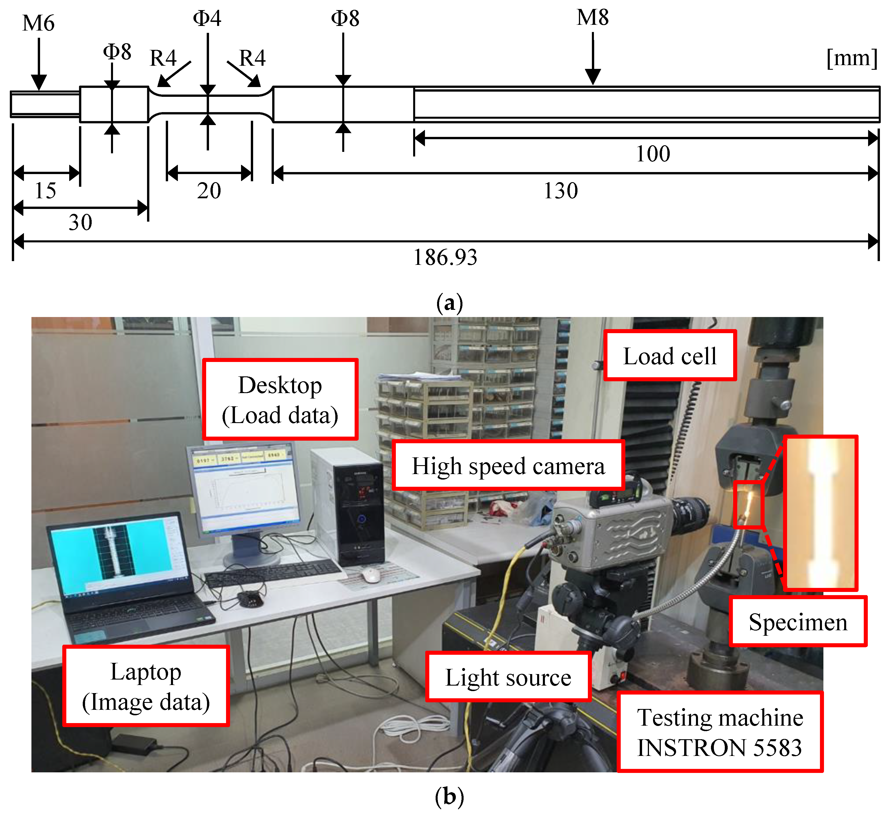
Uniaxial tensile tests were conducted for hardening behavior of the AISI 304 steel in the quasi-static state. Figure 1a shows the drawing of the test specimen of a round bar type dog-bone shape with dimensions, where the gauge length is 20 mm and the diameter of the gauge region is 4 mm. The specimen was also used in intermediate strain rate tests to have consistent results of the hardening curves. The gripping region in the specimen had threads to prevent slip during gripping in the tests. The testing machine was the INSTRON 5583 (Instron, Norwood, MA, USA), whose maximum load capacity was 150 kN and crosshead speed was from 0.05 mm/min to 500 mm/min. Target strain rates were from to in these experiments, and corresponding crosshead speeds were from 1.2 mm/min to 120 mm/min, respectively, for each target strain rate. A high speed camera, Phantom v5 (Phantom, Wayne, NJ, USA), was used to capture images of a speckle pattern during the deformation and Digital Image Correlation (DIC) method was utilized for strain analysis [24,25]. Frame rates were set to 1 fps, 10 fps, and 200 fps for each target strain rate, respectively. Figure 1b shows the experimental setup with the INSTRON 5583 in the quasi-static state case.
2.2. Intermediate Strain Rate Test
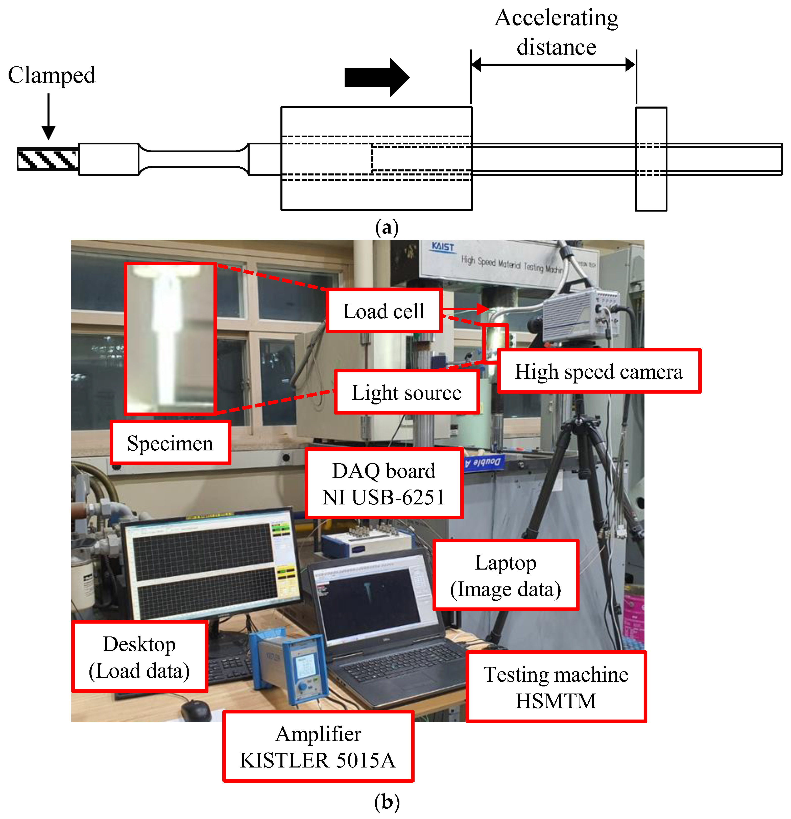
Uniaxial tensile tests were conducted for hardening behavior of the AISI 304 steel at intermediate strain rates with specimens of the same dimensions for the quasi-static state tests, as shown in Figure 1a, to avoid discrepancy in the results due to the difference of the specimen shape. The testing machine was a High Speed Material Testing Machine (HSMTM, KAIST, Daejeon, Korea). The equipment was a servo-hydraulic testing machine with a maximum load capacity of 30 kN and a crosshead speed of 0.003 m/s up to 7.8 m/s. In these tests, the accelerating distance was required so that the crosshead reached the target loading velocity, as described in Figure 2a. Target strain rates were , , and in these experiments and the crosshead speeds were 0.02 m/s, 0.2 m/s, and 2.0 m/s, respectively, for each target strain rate. During the test, deformed images were acquired with a high-speed camera of FASTCAM SA5 (Photron, Tokyo, Japan), because a higher frame rate was required to capture enough number of images of a speckle pattern during the deformation. Frame rates are set to 1000 fps, 10,000 fps, and 25,000 fps respectively for each target strain rate. DIC analysis was also used for strain analysis and Figure 2b shows the experimental setup with the HSMTM in the intermediate strain rate case.
2.3. High Strain Rate Test
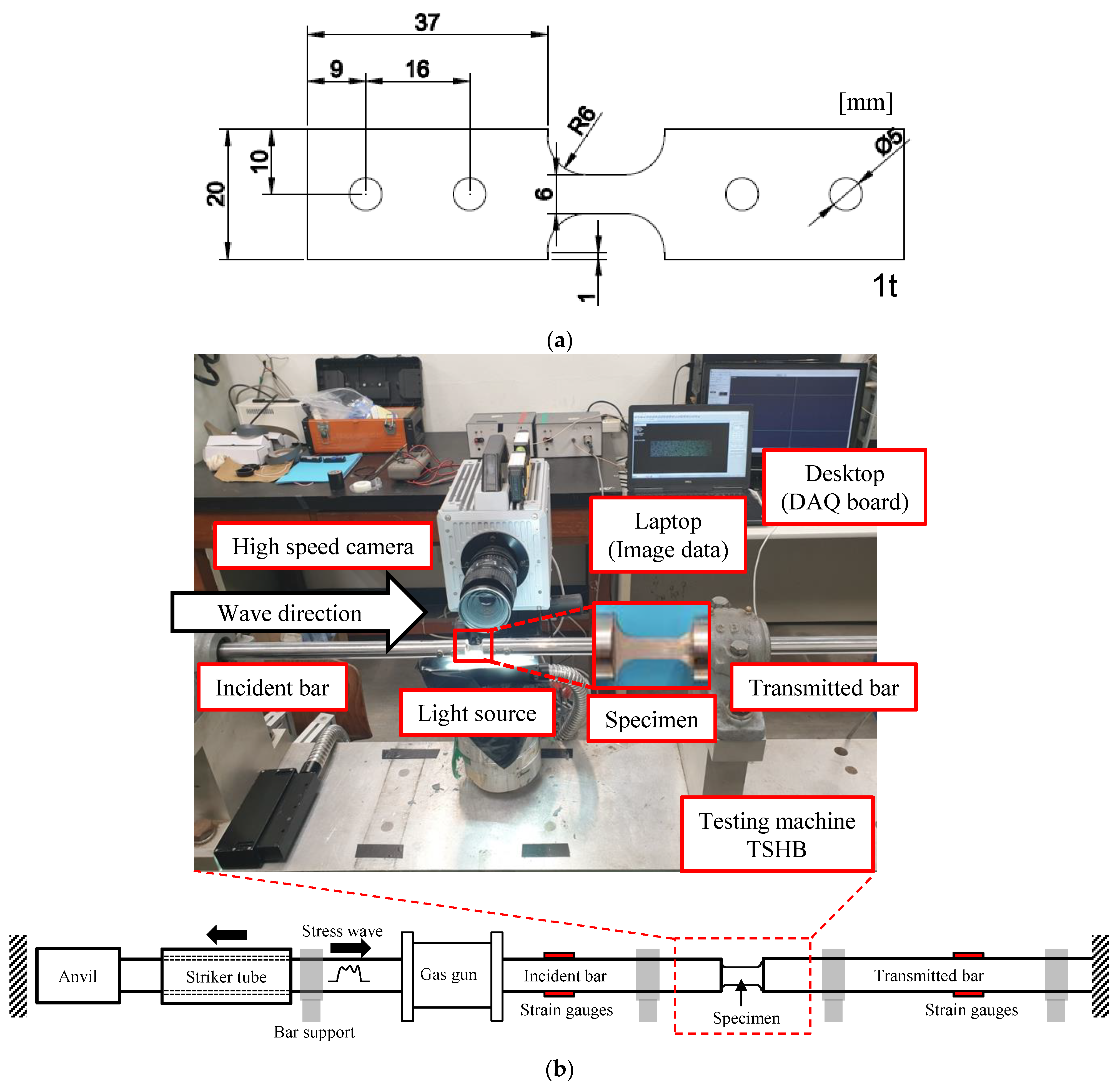
In order to investigate hardening behavior of the AISI 304 steel at high strain rates, a Tensile Split-Hopkinson Bar (TSHB) test was carried out. In the TSHB test, a specimen was deformed by the stress wave induced from the impact between a striker bar and an anvil at the end of an incident bar based on the same principle of a split-Hopkinson pressure bar test. Uniaxial tensile stress and strain were calculated using the reflective wave and the transmitted wave, as below:
where , , and are the elastic modulus, the stress wave velocity, and the cross section area of the transmitted bar or incident bar respectively, and , are the longitudinal length and the cross section area of the specimen, respectively, and and are elastic strains measured at the transmitted bar and the reflected bar respectively. Figure 3a shows the drawing of the TSHB test specimen with the typical geometry [5]. The maximum pressure capacity of the TSHB was about 550 kPa. In the present experiment, a pressure of 138 kPa was applied to induce deformation at a strain rate of , which was enough for the specimen to fracture in the gauge section by the first stress wave. Figure 3b shows the experimental setup with the TSHB in the high strain rate case.
2.4. Ultra-High Strain Rate Test
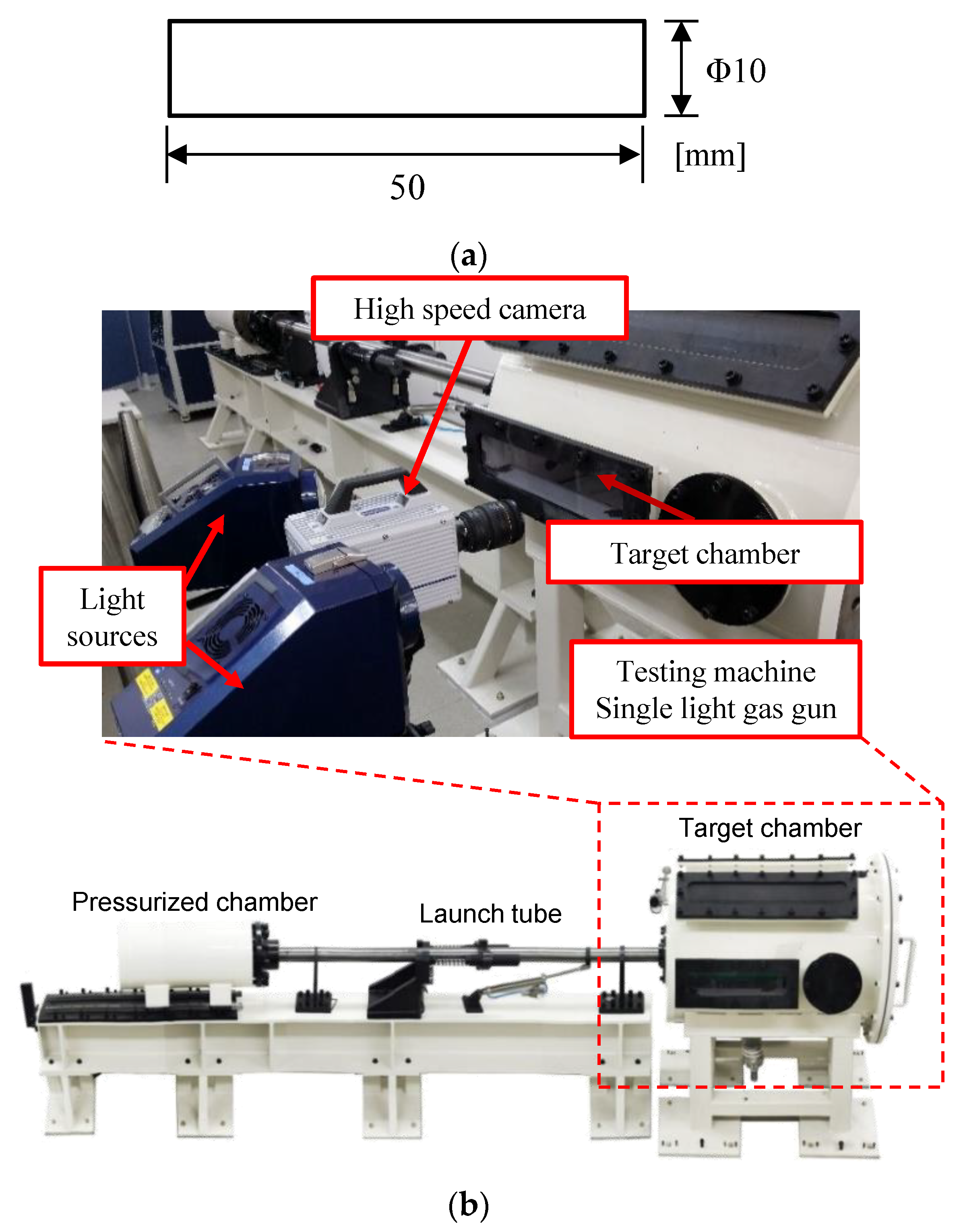
Taylor impact tests are performed to induce deformation of a specimen at ultra-high strain-rate region with a single light gas gun whose maximum pressure capacity is about 13.8 MPa. A specimen of a cylindrical projectile, depicted in Figure 4a, was accelerated by passing through the launch tube and then impacted on the target plate in the target chamber. The target plate was composed of maraging steel in order to be deformed within an elastic region only. Experiments were conducted under an input pressure of 1.57 MPa using nitrogen gas, which derived the impact velocity of the projectile to 224 m/s. Unlike previous tests, it was quite difficult to calculate the stress and strain of a deformed specimen directly from experimental results in the Taylor impact test. Instead, hardening curves at ultra-high strain rates were calibrated by a proper extrapolation method [4,6] as described in the next chapter. In order to apply this method, sequential image series of deformed shapes of a specimen was required for optimization. The sequential images were acquired with a high speed camera of FASTCAM SA5 (Photron, Tokyo, Japan) with frame rates of during the experiments. Figure 4b shows the experimental setup with the Taylor impact testing machine for the deformation at ultra-high strain rates.
3. Results and Discussion
The test results in the previous chapter are evaluated with the following procedures in order to identify hardening curves extended from the quasi-static state up to ultra-high strain rates. Hardening curves ranging from the quasi-static state to high strain-rate region are directly obtained from experiments and are then characterized using the extended Lim–Huh dynamic hardening model. This model shows higher performance with respect to various kinds of materials than other models because it is formulated based on experimental results and their interpolation. A detailed description of the model is presented in Appendix A. Hardening curves at ultra-high strain-rate region are, however, evaluated from an experimental–numerical hybrid inverse optimization process.
3.1. Experimental–Numerical Hybrid Inverse Optimization
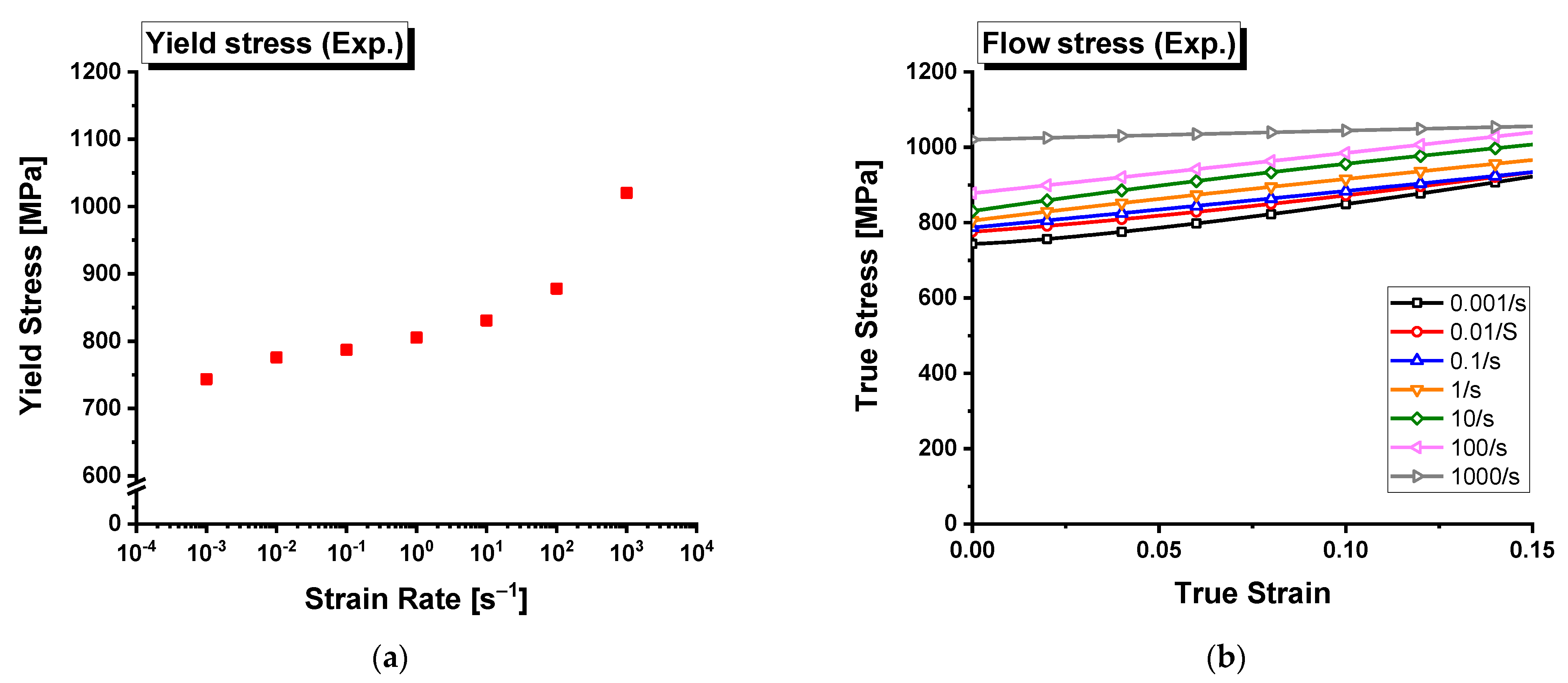
Material tests were conducted at least five times at each strain rate for reproducibility. Stress and strain signals obtained from the tests usually had some undesired signal because of high frequency noise or load ringing phenomenon especially at high strain rates. To remove undesired signals, data conditioning techniques are applied [1,2,25,26]. Then the conditioned signals are fitted using the Swift model [27] by a least square method to define a representative curve at each strain rate. In addition, the yield stress of each strain rate is obtained using a general 0.2% offset method. Figure 5 shows the yield stress and flow stress curves at the strain rates ranging from to . The increase in the yield stress becomes larger as the strain rate increases, but the hardening rate of the flow stress is not remarkable even with large deformation as strain rate increases due to thermal softening effect and dislocation pattern [28]. Thus, the thermal softening effect needs to be considered explicitly when the strain rate of material is high as formulated in Equation (A1) in Appendix A.
The relation between the flow stress from experiments and the isothermal state can be expressed as shown in Equation (2) where the thermal softening effect is formulated with the same manner as explained in Equation (A4) in Appendix A [4,6].
The elevation of temperature of a material during the deformation is calculated as below:
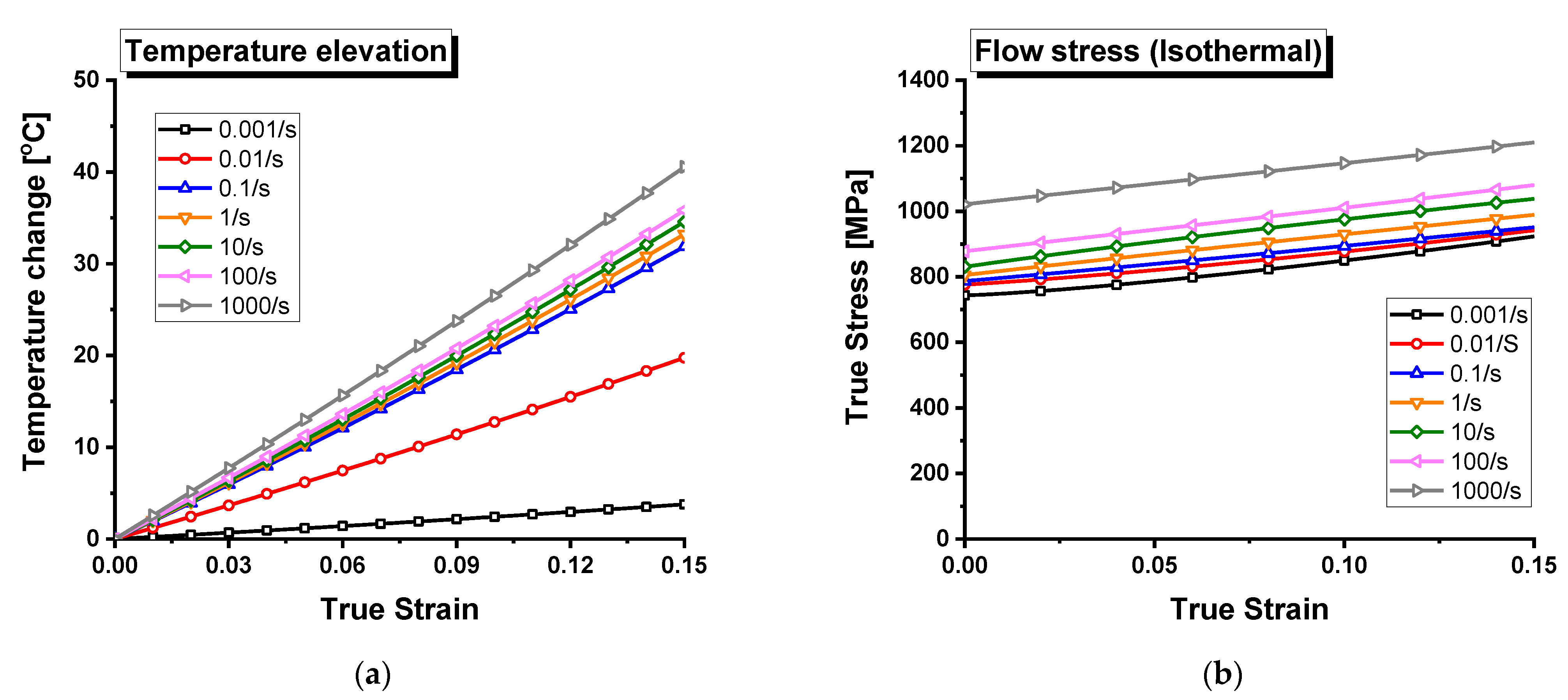
where a conduction factor is the function of strain rate, is the ratio of the transformed heat to the plastic work, is the density, and is the heat capacity of a material. Figure 6a,b show temperature elevation during the deformation and the isothermal flow stress at each strain rate, respectively. The yield stress is not affected by the thermal softening effect because there is no temperature change during the elastic deformation, and the amount of strain hardening in the isothermal state becomes larger than that in the adiabatic state that corresponds to the experimental case in Figure 5b, especially at high strain rates.
The isothermal hardening curves evaluated are represented by the extended Lim–Huh model in Equation (A1) in Appendix A. Hardening curves in the ultra-high strain-rate region are then predicted by extrapolation from the model. Extrapolation, however, may predict incorrect values, which means that the results of the extrapolated values may overestimate or underestimate the yield stress. In order to overcome this pitfall, extrapolated hardening curves need calibration using the experimental results of the Taylor impact test. In this paper, an experimental–numerical hybrid inverse optimization is applied as suggested in the reference [4]. The hardening curves extrapolated are updated by multiplying control factors to current curves to minimize the difference in the deformation shape of a specimen between experimental results and finite element simulation results. Hardening curves at ultra-high strain-rate region are updated with proper iterations as follow:
where and are updated and current flow stress respectively, and and are updated and current yield stress respectively. The instant yield stress is defined in each iteration as follows:
where is the yield stress defined at the reference strain rate of which is set to at room temperature. and in Equation (5) are design variables in the optimization problem. The object function J is defined as a square root of summation of the square of deviations in diameters and lengths of a deformed specimen between experiments and simulation results at each iteration step as below:
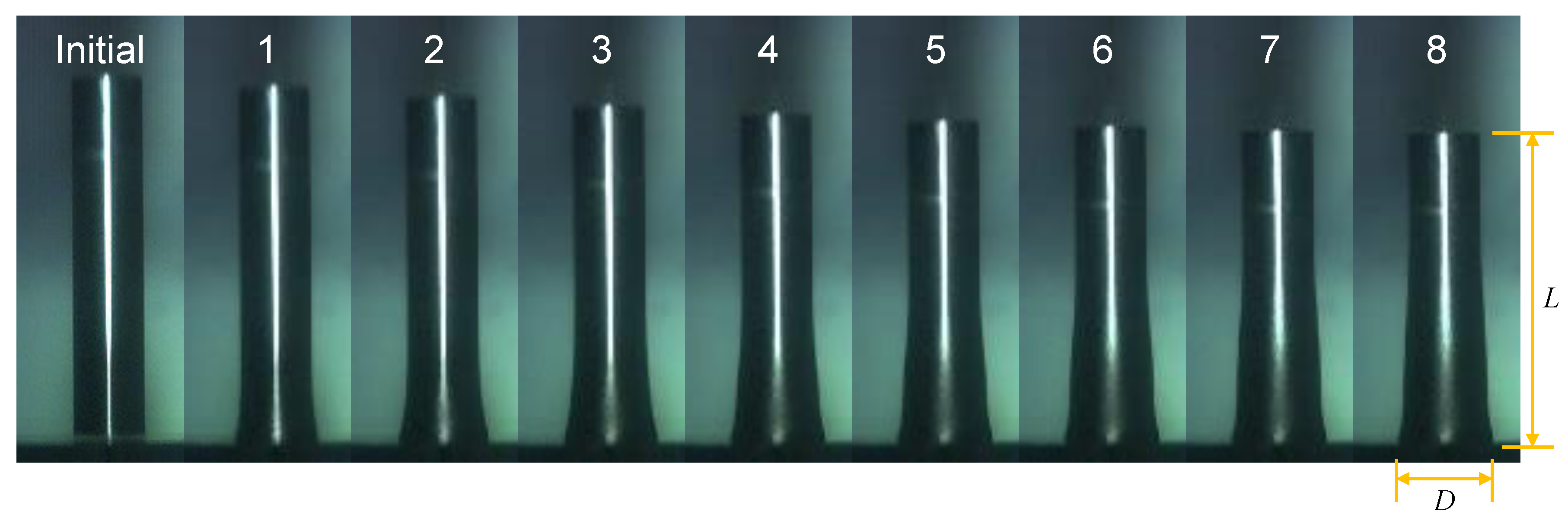
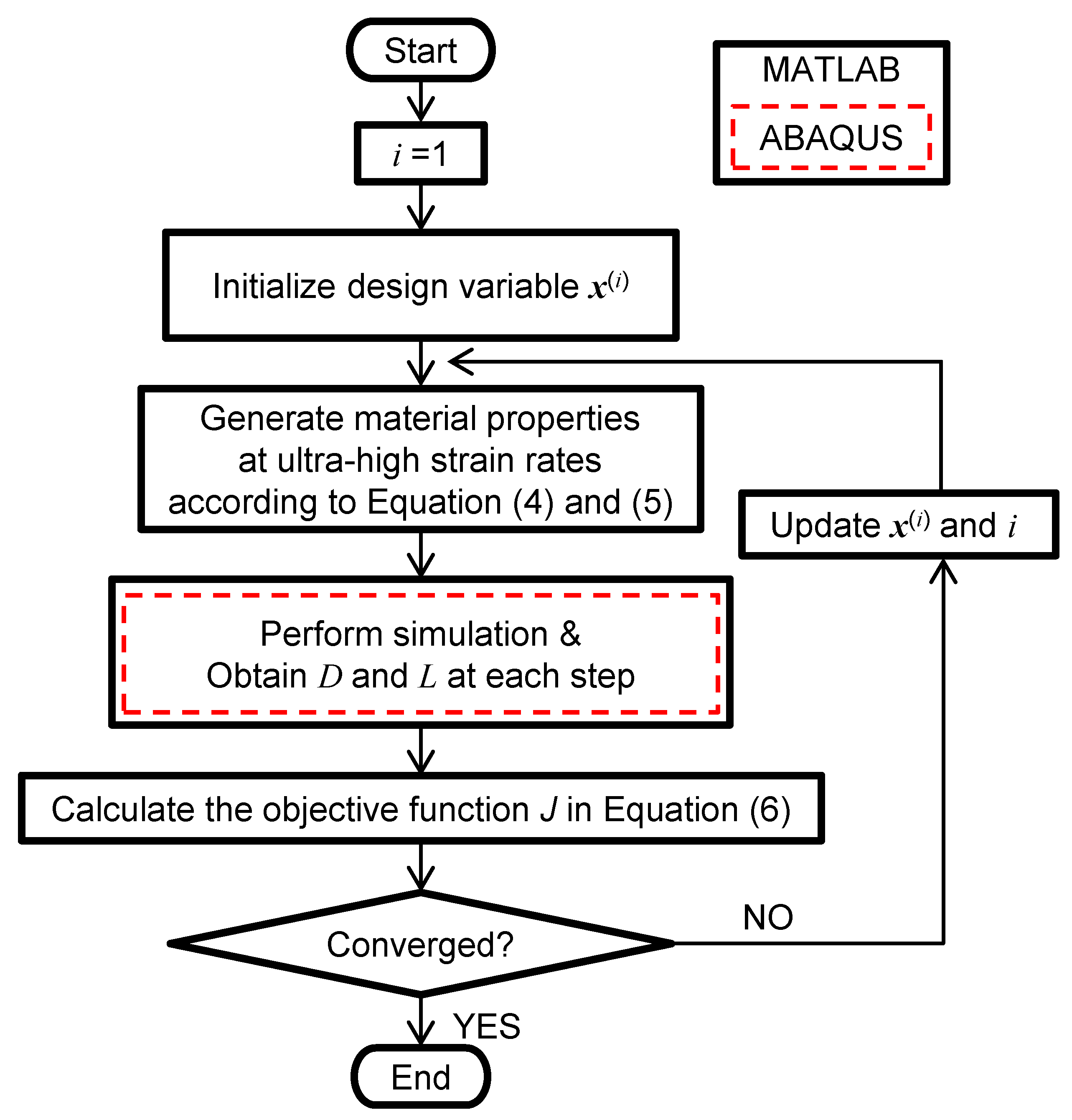
where N is the total number of sequential images compared, D is the diameter of a deformed specimen at the impact surface, and L is the length from the impact surface to the other end of the specimen at each image. Figure 7 shows the sequential deformation images obtained from a Taylor impact test, from which diameters and lengths of a specimen are taken at each image. Optimization iteration is carried out following the flowchart shown in Figure 8 using MATLAB with the Nelder–Mead simplex method. Finite element simulation is performed using a commercial software ABAQUS/Explicit. Finite element simulation condition is described in Figure 9 where a half model is applied to reduce computation time, the impact velocity is 224 m/s, the friction coefficient is 0.1 between the specimen and target surface, and the adiabatic condition are applied. The element types of a specimen and a target are C3D8R with the element sizes of 0.2 mm and 1.0 mm respectively. The total number of nodes is 305,017 and the total number of elements is 285,927. This element size is small enough for finite element simulation results to converge a certain value during high strain rate deformation with thermal softening. The target plate deforms in the elastic state because the maraging steel of the plate has a very high yield strength. Elastic properties and thermal properties of a projectile are shown in Table 1. Figure 10a,b show the variation of the objective function value and design variables during the optimization iteration where the solution process is converged after about 30 iterations. Figure 10c shows the deformation shape of the specimen at each step before and after calibration of the flow stress at the ultra-high strain-rate region compared with experimental points.
3.2. Hardening Curves at a Wide Range of Strain Rates
In order to obtain hardening curves at a wide range of strain rates from the quasi-static state to ultra-high strain rates, various types of material tests are conducted for each strain-rate region and then experimental data are evaluated with proper data processing as mentioned in the previous section.
Figure 11 shows the yield stress at various strain rates and the flow stress curves before and after calibration. Table 2 shows the final results of the material constants of the extended Lim–Huh model. Figure 11a show that the yield stresses are obtained at strain rates of , , and by the extrapolation process and the corresponding values are 1156 MPa, 1446 MPa, and 1943 MPa respectively. The yield stress is then calibrated by the optimization process in the Section 3.1 resulting in 1079 MPa, 1219 MPa, and 1429 MPa respectively. According to the yield stress calibrated, hardening curves at ultra-high strain rates are scaled down by the ratio of 0.9337, 0.8428, and 0.7352 respectively, which are the same ratios as that for the yield stress. Figure 11b shows the hardening curves before calibration and Figure 11c shows the hardening curves after calibration with the same ratios as that for the yield stress. The calibration results reveal that the extrapolation with the extended Lim–Huh model overestimates the hardening behavior and show that the AISI 304 steel has the low strain rate sensitivity compared to the other metals such as AISI 4130 and the Ti6Al4V in the reference [5]. The results imply the tendency that the strain rate sensitivity of the FCC metal is lower than that of the BCC or HCP metal. In addition, this calibration results demonstrate that hardening curves at ultra-high strain rates should be obtained directly from experiments or predicted with proper extrapolation. Figure 11c informs that the yield stress 759 MPa at the quasi-static state increases to 1429 MPa at a strain rate of , which is about 1.9 times of the quasi-static yield stress. It is noted from the results that the difference in hardening curves between the quasi-static state and the high strain rate is severe despite the low strain rate sensitivity. This result suggests that numerical simulation for high-speed deformation requires the consideration of the dynamic material properties.
3.3. Application to Shot Peening Simulation
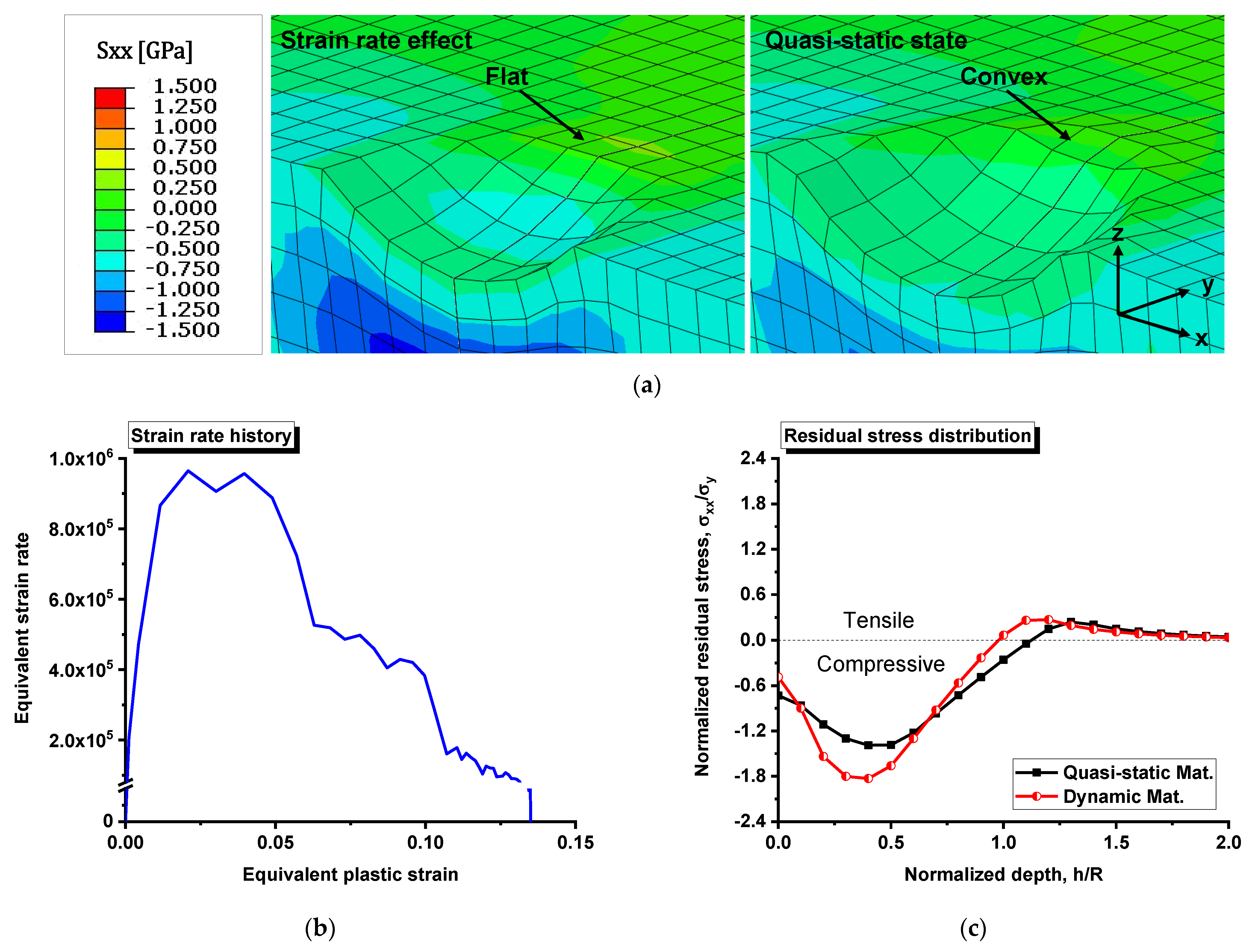
Shot peening is a method to improve surface hardness and fatigue life by inducing compressive residual stress on the material surface, phase transformation from austenite to martensite, and finer grain sizes. In this process, a large number of shots of very small and hard ball-type particles collide to a peen of the surface of the target material with a high impact velocity. This collision induces high strain rate deformation and gradient of plastic deformation which leads to residual stress. Thus, the obtained material properties of the AISI 304 steel considering the strain rate effect are applied to a shot peening simulation and this result is compared with that considering the quasi-static state material properties only. This paper adopts a single shot impingement at the center of the surface and extracts the residual stress profile along the depth direction at the center of the material. Figure 12 shows the finite element model and analysis conditions. A single shot, in which elastic deformation is considered only, impacts the center of the peen at a velocity of 70 m/s. To save computing time, a quarter model is used where symmetric conditions are applied in the x-direction and y-direction. In order to remove stress oscillation, Rayleigh damping coefficients of and are applied to coarse mesh region 2 and the values are referred from [29,30]. The element type C3D8R is adopted for all elements and the element sizes are 0.025 mm in the inner part of the peen region 1 and 0.05 mm in the outer part of the peen region 2. The finite element mesh system consists of the total number of nodes of 36,912 and the total number of elements of 33,175. Elastic material properties used in this simulation to the shot and peen are the same as those in Table 1. Finite element simulation is performed with the commercial software of ABAQUS/Explicit. Figure 13a,c show residual stress distribution contours of with deformation shapes for both cases and the profile of the residual stress along with the depth at the center of the peen. These figures show similar tendencies in stress distribution but difference in magnitude. The maximum compressive residual stress with dynamic material properties is 1.32 times higher than that with the quasi-static properties case. The reason of the difference can be explained as the increase in the flow stress with the increase in the strain rates. When a shot collides the surface of the AISI 304, the material undergoes deformation at high strain rates and the flow stress increases abruptly due to high-speed plastic deformation. As a result, the residual stress increases even for a smaller deformation amount due to high strain rate deformation. This result implies that simulation of high-speed deformation such as shot peening needs to adopt flow stress curves with the strain rate effect for accurate analysis results especially when high strain rate deformation is expected. In addition, it should be taken for granted that the dynamic material properties are necessary in this kind of simulation because the strain rate reaches up to ultra-high strain-rate region as demonstrated in Figure 13b in shot peening simulation.
4. Conclusions
The hardening behavior of the AISI 304 steel is investigated at a wide range of strain rates from the quasi-static state to ultra-high strain rates for simulation of high-speed deformation. Even in high-speed deformation, a set of hardening curves at various strain rates is indispensable for accurate simulation. The conclusions and results are summarized as follows:
- Various experiments were carried out to investigate strain rate hardening behavior with various kinds of testing machines: The INSTORON 5583 for the quasi-static state; the HSMTM for intermediate strain rate tests; the TSHB for the high strain rate tests; and the Taylor impact test for ultra-high strain rate tests. To obtain proper stress–strain curves, the DIC (Digital Image Correlation method) was utilized to obtain the strain during the three tests, which was synchronized with the load. The results from the Taylor impact tests were used to calibrate the stress–strain curves properly at ultra-high strain rates.
- Hardening curves in the quasi-static state and at high strain rates are directly obtained from experiments and those in the ultra-high strain-rate region are evaluated with an experimental–numerical hybrid inverse optimization method by comparison of the simulation result with the experimental result. Hardening curves calibrated demonstrate that the strain rate hardening is lower than extrapolated ones with the extended Lim–Huh model. Thus, the strain rate sensitivity of the AISI 304 steel is less than that predicted from extrapolation of the model and this calibration process is necessary to obtain correct data.
- The novel material properties of the AISI 304 steel at various strain rates are applied to shot peening simulation with a single shot impingement as a demonstration example. The simulation result is compared to the one considering the static properties only. Residual stress distribution shows the similarity in its distribution, but the maximum magnitude of the compressive residual stress shows the difference of 1.32 times higher than that with the static properties. It is concluded from the comparison that the material properties considering the strain rate effect are useful in simulation where high strain rate deformation is expected even for a material which has relatively low strain rate hardening.
Author Contributions
Conceptualization, H.H, R.K., S.L., K.Y., X.A.; formal analysis, S.L., K.Y.; investigation, S.L., K.Y., X.A.; methodology, H.H., R.K., S.L., K.Y.; resources, H.H., R.K., S.L., K.Y., X.A.; writing—original draft, S.L.; writing—review & editing, H.H. All authors have read and agreed to the published version of the manuscript.
Funding
This research received no external funding.
Institutional Review Board Statement
Not applicable.
Informed Consent Statement
Not applicable.
Data Availability Statement
Not applicable.
Conflicts of Interest
The authors declare no conflict of interest.
Nomenclature
| Uniaxial stress, uniaxial strain, and uniaxial strain rate of a specimen in a SHB test | |
| Uniaxial strain of a transmitted bar and a reflected bar in a SHB test | |
| Longitudinal length and cross section area of a gauge region | |
| Elastic modulus, stress wave velocity, and cross section area of a split-Hopkinson bar | |
| Equivalent stress and equivalent strain | |
| Material constants of the Swift hardening model | |
| Material constants for strain rate effect of the Lim–Huh model | |
| Temperature, melting temperature, room temperature, andtemperature change of a specimen | |
| Material constants for thermal softening effect of the extended Lim–Huh model | |
| Stress obtained from experiments and stress in the isothermal state | |
| Material properties for temperature change calculation | |
| Yield stress at a wide range of strain rates and at the reference strain rate for inverse optimization | |
| Reference strain rate for inverse optimization | |
| Objective function for inverse optimization | |
| Deign variables for inverse optimization | |
| Diameter at the contact surface of the specimen in a Taylor impact test from finite element analysis and experiment | |
| Distance from the contact surface to the other end of the specimen in a Taylor impact test from finite element analysis and experiment | |
| HSMTM | High Speed Material Testing Machine, material tests for intermediate strain rates. |
| TSBH | Tensile Split-Hopkinson Bar, material tests for high strain rates. |
Appendix A
The extended Lim–Huh model consists of three terms: a strain hardening term; a strain rate hardening term; and a thermal softening term as below [4,5]:
For the first term of strain hardening in Equation (A1), the Swift model [27] is adopted as follows:
where and are material constants and is the equivalent plastic strain. The strain hardening term for flow stress at the reference strain rate can be replaced by other models such as the Voce model [31], the Hockett–Sherby model [32], or a combination of them depending on the material types.
The second term of strain rate hardening in Equation (A1) is defined as below [12]:
and , and p are material constants, is the strain rate, and is the reference strain rate. This term contains not only strain rate hardening effects but also strain hardening effects to describe shape change of hardening curves with respect to strain rate.
The third term of thermal softening in Equation (A1) is defined as below:
and and are temperatures of the current state, the room temperature, and the melting temperature of the material respectively, and are material constants, and is the reference strain rate. In this paper, material coefficients in Equation (A4) are replaced with those of the AISI 4130 steel from the reference [5].
References
- Huh, H.; Kim, S.-B.; Song, J.-H.; Lim, J.-H. Dynamic tensile characteristics of TRIP-type and DP-type steel sheets for an auto-body. Int. J. Mech. Sci. 2008, 50, 918–931. [Google Scholar] [CrossRef]
- Huh, H.; Lim, J.; Park, S. High speed tensile test of steel sheets for the stress-strain curve at the intermediate strain rate. Int. J. Automot. Technol. 2009, 10, 195–204. [Google Scholar] [CrossRef]
- Zhao, H.; Gary, G. On the use of SHPB techniques to determine the dynamic behavior of materials in the range of small strains. Int. J. Solids Struct. 1996, 33, 3363–3375. [Google Scholar] [CrossRef]
- Piao, M.; Huh, H.; Lee, I.; Ahn, K.; Kim, H.; Park, L. Characterization of flow stress at ultra-high strain rates by proper extrapolation with Taylor impact tests. Int. J. Impact Eng. 2016, 91, 142–157. [Google Scholar] [CrossRef]
- Piao, M.; Huh, H.; Lee, I.; Park, L. Characterization of hardening behaviors of 4130 Steel, OFHC Copper, Ti6Al4V alloy considering ultra-high strain rates and high temperatures. Int. J. Mech. Sci. 2017, 131, 1117–1129. [Google Scholar] [CrossRef]
- Lee, S.; Huh, H. Shear Stress Hardening Curves of AISI 4130 Steel at Ultra-high Strain Rates with Taylor Impact Tests. Int. J. Impact Eng. 2021, 149, 103789. [Google Scholar] [CrossRef]
- Carbonniere, J.; Thuillier, S.; Sabourin, F.; Brunet, M.; Manach, P.-Y. Comparison of the work hardening of metallic sheets in bending–unbending and simple shear. Int. J. Mech. Sci. 2009, 51, 122–130. [Google Scholar] [CrossRef]
- Thuillier, S.; Manach, P.-Y. Comparison of the work-hardening of metallic sheets using tensile and shear strain paths. Int. J. Plast. 2009, 25, 733–751. [Google Scholar] [CrossRef]
- Lou, Y.; Yoon, J.W.; Huh, H. Modeling of shear ductile fracture considering a changeable cut-off value for stress triaxiality. Int. J. Plast. 2014, 54, 56–80. [Google Scholar] [CrossRef]
- Johnson, G.R. A constitutive model and data for materials subjected to large strains, high strain rates, and high temperatures. In Proceedings of the 7th International Symposium of Ballistics, The Hague, The Netherlands, 19–21 April 1983; pp. 541–547. [Google Scholar]
- Khan, A.S.; Huang, S. Experimental and theoretical study of mechanical behavior of 1100 aluminum in the strain rate range 10− 5− 104s− 1. Int. J. Plast. 1992, 8, 397–424. [Google Scholar] [CrossRef]
- Huh, H.; Ahn, K.; Lim, J.H.; Kim, H.W.; Park, L.J. Evaluation of dynamic hardening models for BCC, FCC, and HCP metals at a wide range of strain rates. J. Mater. Processing Technol. 2014, 214, 1326–1340. [Google Scholar] [CrossRef]
- Kang, W.; Cho, S.; Huh, H.; Chung, D. Modified Johnson-Cook model for vehicle body crashworthiness simulation. Int. J. Veh. Des. 1999, 21, 424–435. [Google Scholar] [CrossRef]
- Taylor, G.I. The use of flat-ended projectiles for determining dynamic yield stress I. Theoretical considerations. Proc. R. Soc. Lond. Ser. A Math. Phys. Sci. 1948, 194, 289–299. [Google Scholar]
- Sabioni, A.C.S.; Huntz, A.-M.; Luz, E.C.d.; Mantel, M.; Haut, C. Comparative study of high temperature oxidation behaviour in AISI 304 and AISI 439 stainless steels. Mater. Res. 2003, 6, 179–185. [Google Scholar] [CrossRef] [Green Version]
- Park, W.S.; Yoo, S.W.; Kim, M.H.; Lee, J.M. Strain-rate effects on the mechanical behavior of the AISI 300 series of austenitic stainless steel under cryogenic environments. Mater. Des. 2010, 31, 3630–3640. [Google Scholar] [CrossRef]
- Zheng, C.; Yu, W. Effect of low-temperature on mechanical behavior for an AISI 304 austenitic stainless steel. Mater. Sci. Eng. A 2018, 710, 359–365. [Google Scholar] [CrossRef]
- Wu, J.; Liu, H.; Wei, P.; Zhu, C.; Lin, Q. Effect of shot peening coverage on hardness, residual stress and surface morphology of carburized rollers. Surf. Coat. Technol. 2020, 384, 125273. [Google Scholar] [CrossRef]
- Webster, G.; Ezeilo, A. Residual stress distributions and their influence on fatigue lifetimes. Int. J. Fatigue 2001, 23, 375–383. [Google Scholar] [CrossRef]
- Wohlfahrt, H. The influence of peening conditions on the resulting distribution of residual stress. In Proceedings of the Second International Conference on Shot Peening, Chicago, IL, USA, 14–17 May 1984; pp. 316–331. [Google Scholar]
- Meguid, S.; Shagal, G.; Stranart, J.; Daly, J. Three-dimensional dynamic finite element analysis of shot-peening induced residual stresses. Finite Elem. Anal. Des. 1999, 31, 179–191. [Google Scholar] [CrossRef]
- Schiffner, K. Simulation of residual stresses by shot peening. Comput. Struct. 1999, 72, 329–340. [Google Scholar] [CrossRef]
- Guagliano, M. Relating Almen intensity to residual stresses induced by shot peening: A numerical approach. J. Mater. Processing Technol. 2001, 110, 277–286. [Google Scholar] [CrossRef]
- Pan, B.; Qian, K.; Xie, H.; Asundi, A. Two-dimensional digital image correlation for in-plane displacement and strain measurement: A review. Meas. Sci. Technol. 2009, 20, 062001. [Google Scholar] [CrossRef]
- Choi, M.; Huh, H.; Jeong, S.; Kim, C.; Chae, K. Measurement uncertainty evaluation with correlation for dynamic tensile properties of auto-body steel sheets. Int. J. Mech. Sci. 2017, 130, 174–187. [Google Scholar] [CrossRef]
- Huh, H.; Jeong, S.; Bahng, G.; Chae, K.; Kim, C. Standard uncertainty evaluation for dynamic tensile properties of auto-body steel-sheets. Exp. Mech. 2014, 54, 943–956. [Google Scholar] [CrossRef]
- Swift, H. Plastic instability under plane stress. J. Mech. Phys. Solids 1952, 1, 1–18. [Google Scholar] [CrossRef]
- Huh, H.; Yoon, J.-H.; Park, C.-G.; Kang, J.-S.; Huh, M.-Y.; Kang, H.-G. Correlation of microscopic structures to the strain rate hardening of SPCC steel. Int. J. Mech. Sci. 2010, 52, 745–753. [Google Scholar] [CrossRef]
- Gariépy, A.; Larose, S.; Perron, C.; Lévesque, M. Shot peening and peen forming finite element modelling–towards a quantitative method. Int. J. Solids Struct. 2011, 48, 2859–2877. [Google Scholar] [CrossRef]
- Gariépy, A.; Miao, H.; Lévesque, M. Simulation of the shot peening process with variable shot diameters and impacting velocities. Adv. Eng. Softw. 2017, 114, 121–133. [Google Scholar] [CrossRef]
- Voce, E. The relationship between stress and strain for homogeneous deformation. J. Inst. Met. 1948, 74, 537–562. [Google Scholar]
- Hockett, J.; Sherby, O. Large strain deformation of polycrystalline metals at low homologous temperatures. J. Mech. Phys. Solids 1975, 23, 87–98. [Google Scholar] [CrossRef]
Figure 1.
Material tests in the quasi-static state: (a) Dimensions of the specimen; (b) Experimental setup with the INSTRON 5583. (Adapted from ref. [6]).
Figure 1.
Material tests in the quasi-static state: (a) Dimensions of the specimen; (b) Experimental setup with the INSTRON 5583. (Adapted from ref. [6]).

Figure 2.
Material tests at intermediate strain rates: (a) Loading mechanism; (b) Experimental setup with the HSMTM. (Adapted from ref. [6]).
Figure 2.
Material tests at intermediate strain rates: (a) Loading mechanism; (b) Experimental setup with the HSMTM. (Adapted from ref. [6]).

Figure 3.
Material tests at high strain rates: (a) Drawing of the specimen; (b) Experimental setup with the TSHB.
Figure 3.
Material tests at high strain rates: (a) Drawing of the specimen; (b) Experimental setup with the TSHB.

Figure 4.
Taylor impact tests for deformation at ultra-high strain rates: (a) Drawing of a specimen; (b) Experimental setup with the Taylor impact testing machine. (Adapted from ref. [6]).
Figure 4.
Taylor impact tests for deformation at ultra-high strain rates: (a) Drawing of a specimen; (b) Experimental setup with the Taylor impact testing machine. (Adapted from ref. [6]).

Figure 5.
Experimental results at strain rates ranging from to : (a) Yield stress; (b) Flow stress curve.
Figure 5.
Experimental results at strain rates ranging from to : (a) Yield stress; (b) Flow stress curve.

Figure 6.
Temperature elevation and flow stress in the isothermal state at strain rates ranging from to : (a) Temperature elevation; (b) Flow stress in the isothermal state.
Figure 6.
Temperature elevation and flow stress in the isothermal state at strain rates ranging from to : (a) Temperature elevation; (b) Flow stress in the isothermal state.

Figure 7.
Sequential deformed images taken from a Taylor impact test.

Figure 8.
Flow chart of the optimization process for the calibration of hardening behavior at ultra-high strain-rate region. (Adapted from ref. [6]).
Figure 8.
Flow chart of the optimization process for the calibration of hardening behavior at ultra-high strain-rate region. (Adapted from ref. [6]).

Figure 9.
Finite element mesh system and simulation conditions in the calibration of hardening behavior at ultra-high strain-rate region.
Figure 9.
Finite element mesh system and simulation conditions in the calibration of hardening behavior at ultra-high strain-rate region.

Figure 10.
Optimization results for the calibration of hardening behavior at ultra-high strain-rate region: (a) Convergence of the objective function; (b) Convergence of design variables; (c) Deformation image series before and after calibration with experimental points.
Figure 10.
Optimization results for the calibration of hardening behavior at ultra-high strain-rate region: (a) Convergence of the objective function; (b) Convergence of design variables; (c) Deformation image series before and after calibration with experimental points.

Figure 11.
Calibrated yield stress and flow stress at ultra-high strain-rate region: (a) Yield stress before and after calibration; (b) Flow stress before calibration; (c) Flow stress after calibration.
Figure 11.
Calibrated yield stress and flow stress at ultra-high strain-rate region: (a) Yield stress before and after calibration; (b) Flow stress before calibration; (c) Flow stress after calibration.

Figure 12.
Finite element mesh system and simulation conditions for the shot-peening simulation.

Figure 13.
Finite element analysis results of shot peening simulation with the flow stress of the quasi-static state and considering strain rate effect: (a) Residual stress distribution contours and deformation shapes; (b) Strain rate history underneath the center; (c) Residual stress profiles along with the depth at the center.


Table 2.
Material constants for AISI 304 steel determined with the extended Lim–Huh model [5].
Table 2.
Material constants for AISI 304 steel determined with the extended Lim–Huh model [5].
| Material Constant | Value | Material Constant | Value |
|---|---|---|---|
Publisher’s Note: MDPI stays neutral with regard to jurisdictional claims in published maps and institutional affiliations. |
© 2022 by the authors. Licensee MDPI, Basel, Switzerland. This article is an open access article distributed under the terms and conditions of the Creative Commons Attribution (CC BY) license (https://creativecommons.org/licenses/by/4.0/).
Share and Cite
MDPI and ACS Style
Lee, S.; Yu, K.; Huh, H.; Kolman, R.; Arnoult, X. Dynamic Hardening of AISI 304 Steel at a Wide Range of Strain Rates and Its Application to Shot Peening Simulation. Metals 2022, 12, 403. https://doi.org/10.3390/met12030403
AMA Style
Lee S, Yu K, Huh H, Kolman R, Arnoult X. Dynamic Hardening of AISI 304 Steel at a Wide Range of Strain Rates and Its Application to Shot Peening Simulation. Metals. 2022; 12(3):403. https://doi.org/10.3390/met12030403
Chicago/Turabian StyleLee, Sungbo, Kwanghyun Yu, Hoon Huh, Radek Kolman, and Xavier Arnoult. 2022. "Dynamic Hardening of AISI 304 Steel at a Wide Range of Strain Rates and Its Application to Shot Peening Simulation" Metals 12, no. 3: 403. https://doi.org/10.3390/met12030403
Note that from the first issue of 2016, this journal uses article numbers instead of page numbers. See further details here.