Application of Tanks-in-Series Model to Characterize Non-Ideal Flow Regimes in Continuous Casting Tundish

Abstract

This study describes a new tanks-in-series model for analyzing non-ideal flow regimes in a single-strand tundish. The tundish was divided into two interconnected tanks, namely an inlet tank and an outlet tank. A water model experiment was carried out to separately measure the residence-time distribution (RTD) of the two tanks. Drift beads were adopted in the water model experiment to simulate the non-metallic inclusions in molten steel. Dead volume fraction was evaluated by analyzing measured RTD curves. The ratio between mixed flow volume and plug flow volume was proposed as a new criterion to evaluate the inclusion removal. In the inlet tank, a higher mixed flow fraction was preferred to effectively release turbulent kinetic energy and enhance inclusion collision growth. In the outlet tank, a higher plug flow fraction was preferred to facilitate inclusion removal by flotation. The optimal positions of the weir were recommended based on the RTD analysis and the inclusion removal from the results of water model experiments. A theoretical equation was derived based on the tanks-in-series model, providing a good fitting function to analyze the experimental data. The confirmation test was performed by applying computational fluid dynamics simulations of liquid steel flow in the real tundish.

1. Introduction

The initial idea of using residence-time distribution (RTD) in the analysis of a chemical reactor’s performance was proposed by MacMullin and Weber in 1935 [1]. An extensive study of mixing performance in non-ideal reactors using RTD theory was published by Danckwert in 1953 [2]. Since then, RTD theory based on the tracer technology has become an important tool for the analysis of industrial reactors. It has been widely utilized in industry to optimize processes, improve product quality, save energy and reduce pollution [3]. Metallurgical reactor was identified as an appropriate target beneficiary for applying RTD theory since metal industries are globally widespread and are of considerable economic and environmental importance.

Steelmaking tundish acts as a reservoir and distributor settled between the ladle and the continuous casting molds. With the emphasis on the steel quality, a modern tundish is designed to provide maximum opportunity for the control of liquid flow, mixing and inclusion removal [4,5]. The RTD characteristics of a given tundish can be studied through the pulse injection of inert tracer at the vessel inlet and monitoring its concentration change at the vessel outlet. RTD analyses such as mean residence time, plug flow volume, dead zone volume and mixed flow volume can be used to estimate the tundish performance [6,7,8]. Two responses are typically applied, namely (i) inclusion remove rate, (ii) dead volume fraction. The proper implementation of flow control devices (FCD) in the tundish ensures the increase of inclusion removal rate and the decrease of dead volume fraction [9,10].

A large number of studies about mathematical models and water models have been reported on the analyses of RTD with a focus on the optimization of flow control device in a tundish. A summary of the previous modelling works for RTD studies can be found in

Table 1. Summary of modeling investigations on residence-time distribution (RTD) in the tundish.

Reference	Model 1	Code	Design			Numeric Model 5	RTD 6	Perfor. Criteria 7	RTD Model 8	Parameter Study 9
			Str. 2	Fluid 3	FCD 4	Fluid/Turb./Inc.
López-Ramirez (1998) [11]	N	-	2	S	B, TI	k-ε	E	DV,PV,MV	SG	SFR, FCD, TC
Craig (2001) [12]	N	FLUENT	1	S,W	D,W	k-ε	E	DV	SG	FCD
Jha (2004) [13]	N	PHOENICS	6	S	TI	(vari.)	E	DV,PV,MV	SG	TC, FCD
Vargas-Zamora (2004) [14]	P	-	1	W	TI, D	-	F	DV,PV,MV	SG	GFR
Zhong (2008) [15]	P	-	2	W	TI, D, W	-	E	DV,PV,PV/DV	SG	TC, FCD, GFR
Kumar (2008) [16]	N,P	FLUENT	4	W	TI,D	k-ε	E	DV,PV,MV	SG	TC,FCD
Bensouici (2009) [17]	N, P	FLUENT	1	W	W, D	k-ε	E	DV,PV,MV	SG	MS, FCD
Yang (2009) [18]	N,P,I	FLUENT	2	W,S	D,TI	k-ε	E	DV,PV,MV	SG	TC,FCD,IS
Cwudziński (2010) [19]	N,I	FLUENT	1	S	D,TI	k-ε	E,F	DV,PV,MV	SG	GFR,FCD
Zheng (2011) [20]	N, I	CFX	2	S	TI, B	E/k-ε/L	E	DV,PV,MV	SG	TC, GFR, IS
Tripathi (2012) [21]	N	FLUENT	1	S	TI, ED	k-ε	E	DV,PV,PV/DV	SG	FCD
Chen (2014) [22]	N, P	FLUENT	1	S, W	W	E/k-ε/L	E	DV,PV,MV	SG	TC, FCD, IS
Chen (2015) [23]	N, P	FLUENT	1	W	SR, D, W, TI	(vari.)	E	DV	SG	MS, TS, TP
Chang (2015) [24]	N, P	FLUENT	7	S, W	TI, B	E/k-ε/L	E	DV,PV,MV	SG	GFR, FCD
Devi (2015) [25]	N, P	FLUENT	2	S, W	D	E/k-ε	E	PV/DV,PV/MV	SG	FCD, GFR
He (2016) [26]	N, P	FLUENT	5	S, W	TI, B	k-ε	E	DV,PV,MV	SG	TC, SFR
Neves (2017) [26]	N, P	CFX	2	W	SR, D, W	E/k-ε	E	DV,PV,MV	SG	GFR, FCD
Aguilar–Rodriguez (2018) [28]	N	FLUENT	1	S	-	VOF	E	DV,PV,MV	SG	GFR, TC, FCD
Yang (2019) [29]	N	CFX	2	S	D, TI	k-ε/L	E	DV,PV,MV	SG	FCD, TC
Wang (2020) [30]	N	FLUENT	2	S	W, TI, F	E/k-ε/L	E	DV,PV,MV	SG	IS, FCD, TC
Tkadlečková [31]	N	FLUENT	5	S	TI,	k-ε/L	F	DV,PV,MV	SG	FCD,IS

¹ N—numeric model; P—physical model; ² Str.: strand; ³ W—water; S—steel; ⁴ FCD—flow control devices; SR—stop rod; D—dam; ED—electromagnetic dam; W—weir; TI—Turbulence inhibitor; F—filter; B—baffles; ⁵ Turbu.: turbulence; Inc.: Inclusion; E—Eulerian; VOF—volume of fluid; ⁶ E—E-curve; F—F-curve. ⁷ Perfor.: performance; DV—dead volume; PV—plug flow volume; MV—mixed flow volume; ⁸ SG: single model; SZ: series model; ⁹ SFR—steel flow rate; GFR—gas flow rate; TC—tundish configuration; MS—mesh size; TS—time step; ID—inlet depth; IS—inclusion size; FCD—flow control devices.

[11,12,13,14,15,16,17,18,19,20,21,22,23,24,25,26,27,28,29,30,31]. These modelling studies led to considerable improvements in understanding the various flow phenomena associated with the tundish operations. Among them, the single-tank model was applied by analyzing RTD curves at the outlet of the tundish, as listed in column-RTD model. Most calculated the dead volume fraction, the plug volume fraction and the mixed volume fractions in the tundish. The tundish performance criteria were mainly based on the dead volume faction.

However, the dead volume fraction is not the sole criterion. The ratio of plug flow volume and mixed flow volume is also very important to analyze the tundish performance, e.g., mixing and inclusion removal. With the installation of FCD, it is difficult to describe the local flow patterns by using the single-tank model. With this consideration, an entire tundish can be divided into a series of interacting tanks with different metallurgical functions. For instance, a single-strand tundish can be divided into two interacting tanks (inlet tank and outlet tank) in series due to the configuration of the weir. The ratio of plug flow volume and mixed flow volume in the inlet tank and outlet tank changes over the location and height of the weir. In the inlet tank, to effectively release turbulent kinetic energy and to promote the collision growth of inclusions, a large mixed flow volume is preferred. In the outlet tank, to facilitate inclusion floatation removal with a stable horizontal flow pattern of liquid steel, a large plug flow volume is preferred.

Therefore, a new tanks-in-series model for analyzing the non-ideal flow regimes in a single-strand tundish was developed in this study. Water model experiment was conducted to measure RTD curves of the two interconnected tanks. Drift beads were adopted in the water model experiment to simulate the non-metallic inclusions in molten steel. Inclusion removal rate and dead volume fraction were studied by the influence of location and height of the weir. The ratio of mixed flow volume and plug flow volume in the two tanks was systematically analyzed. The optimal position of the weir was proposed from the results of water model experiment. A confirmation test was performed by applying the computational fluid dynamics (CFD) simulation in the real tundish.

2. Model Description

2.1. Theoretical Model

2.1.1. Single-Tank Model

The liquid steel in tundish has non-uniform flow patterns due to the existence of short-circuiting flow, cyclic flow and stagnant zone. Therefore, a single-tank model was appropriate to analyze the non-ideal flow in the entire tundish. This model was based on the assumption that the tundish contains three different flow regimes: plug flow, mixed flow and dead zone. RTD was applied to characterize the volume of different flow regimes (V_p, V_m and V_d).

RTD is a statistical representation of the time spent by an arbitrary volume of the fluid in the tundish. It is defined as the exit age distribution in the form of E(t) for a pulse input. E-curve can be plotted based on the dimensionless outlet concentration (C-curve) measured in the water model or calculated by the mathematical model. Actual mean residence time ($\overline{\tau })$ is presented in Equation (1) [32].

$$\overline{\tau }=\frac{{{\displaystyle \int }}_0^{\infty }tC\left(t\right)dt}{{{\displaystyle \int }}_0^{\infty }C\left(t\right)dt}$$

(1)

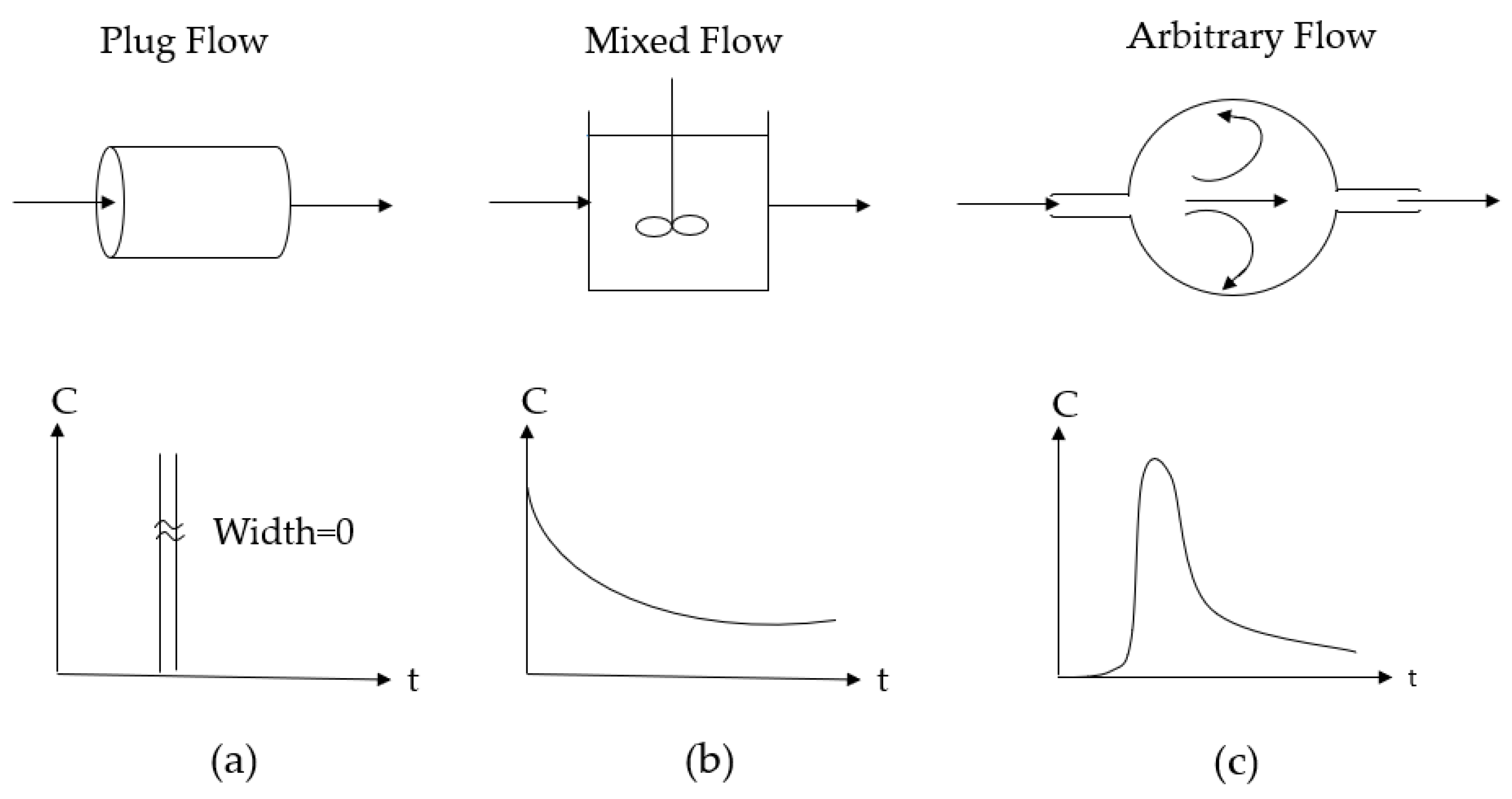
In a plug flow reactor, as exhibits in Figure 1a, the response to a pulse input is that all fluid elements leave the vessel with the same residence time. In a completely mixed flow reactor, as shown in Figure 1b, the fluid elements leave the vessel over a range of residence time. When a device operates between these two conditions, there is a degree of plug flow that results in an initial monitored concentration peak at the outlet, and a degree of mixed flow that results in the concentration tails at the outlet, as presented in Figure 1c [33].

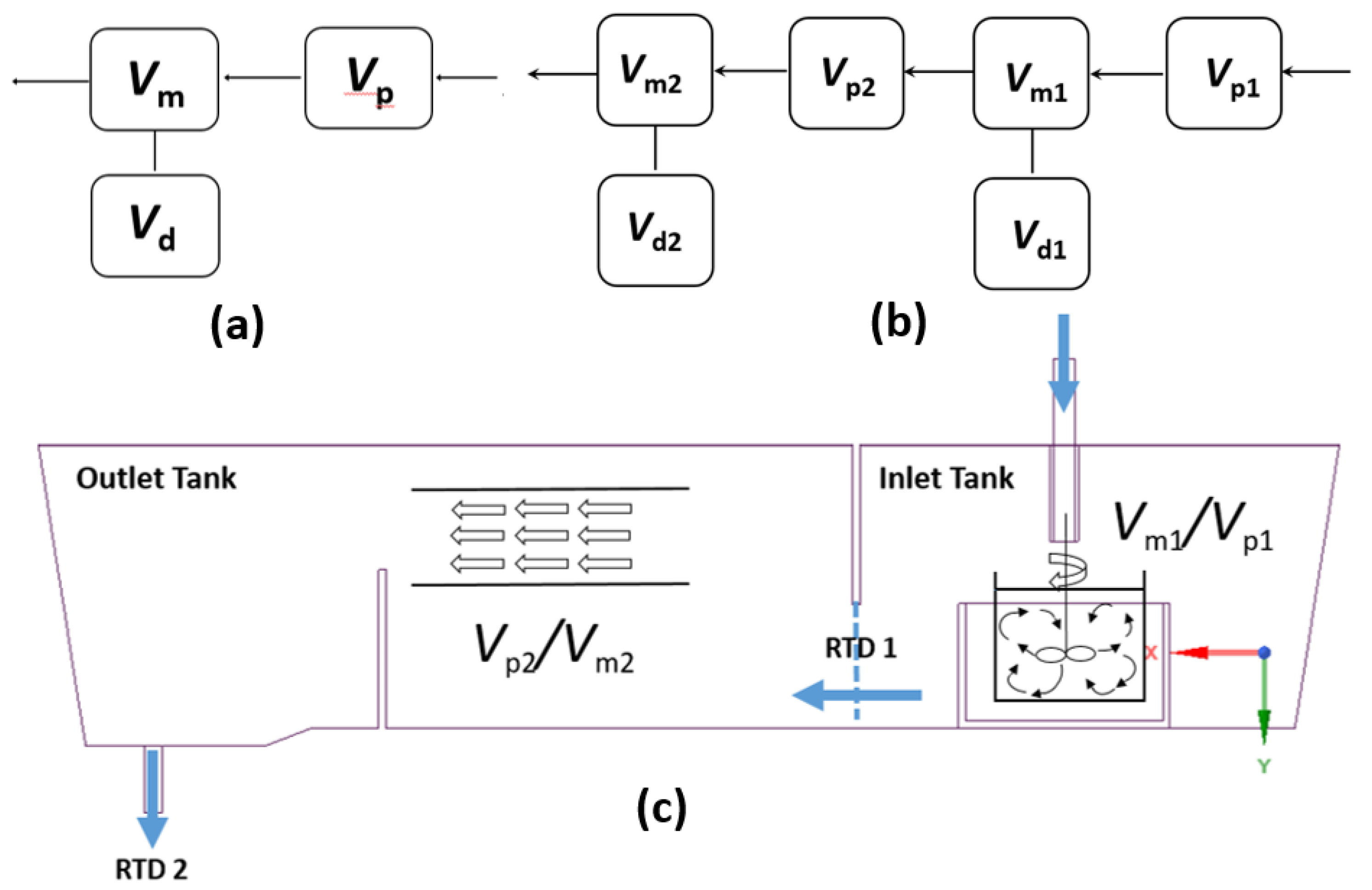
Applying the single-tank model of tundish (as shown in Figure 2a), plug flow volume fraction (V_p/V), mixed flow volume fraction (V_m/V) and dead volume fraction (V_d/V) were calculated through Equations (2)–(4) [13].

Dead volume fraction,

$$V_{\mathrm{d}}/V=1-\frac{\overline{\tau }}{\tau }$$

(2)

Plug flow volume fraction,

$$V_{\mathrm{P}}/V=\left({\theta }_{\min }+{\theta }_{\mathrm{peak}}\right)/2$$

(3)

Mixed flow volume fraction,

$$V_{\mathrm{m}}/V=1-V_{\mathrm{d}}/V-V_{\mathrm{p}}/V$$

(4)

where, τ is the theoretical residence time, θ_min is the dimensionless time of minimum concentration at the tundish outlet, θ_peak is the dimensionless time of peak concentration at the tundish outlet.

Applying the single-tank model, the theoretical E-curve can be expressed as a combination of different flow regimes, as given in Equation (5) [34].

$$\mathrm{E}(\theta )=\{\begin{array}{cc}0,& 0\le \theta \le \frac{V_{\mathrm{p}}}{V}\\ \frac{V}{V_{\mathrm{m}}}{e}^{\left(-\frac{V}{V_{\mathrm{m}}}\theta +\frac{V_{\mathrm{p}}}{V_{\mathrm{m}}}\right)},& \theta \ge \frac{V_{\mathrm{p}}}{V}\end{array}$$

(5)

2.1.2. Tanks-in-Series Model

As illustrated in Figure 2b,c, the tundish was divided into two interacting tanks in series (inlet tank and outlet tank) based on the configuration of the weir. In the single-tank model, the dead volume fraction was calculated for the entire tundish. It is difficult to determine whether the dead volume exists mainly in the inlet tank or in the outlet tank. Hence, a detailed theoretical model, e.g., tanks-in-series model, was proposed to characterize the flow regimes in the tundish [35].

The mass balance equation of tracer for the ith tank in a system is defined as:

$$F_{\mathrm{V}}\cdot C_{i-1}\left(t\right)-F_{\mathrm{V}}\cdot C_i\left(t\right)=V_i\cdot \frac{\mathrm{d}{C}_i\left(t\right)}{\mathrm{d}t}$$

(6)

$$\frac{\mathrm{d}{C}_i\left(t\right)}{\mathrm{d}t}+\frac{C_i\left(t\right)}{{\tau }_i}=\frac{1}{{\tau }_i}\cdot C_{i-1}\left(t\right)$$

(7)

For pulse input of tracer, the initial conditions for the inlet tank (the 1st tank) are

$$C_0=0,C_1\left(0\right)=\frac{M}{V_{\mathrm{m}1}}$$

(8)

The following expression for the tracer concentration with the time in the inlet tank can be derived by integrating Equation (7) over the initial conditions.

$$C_1\left(t\right)=\frac{M}{V_{\mathrm{m}1}}\cdot e^{-\frac{t}{{\tau }_1}}$$

(9)

The mass balance equation of tracer in the outlet tank is expressed as:

$$\frac{\mathrm{d}{C}_2\left(t\right)}{\mathrm{d}t}+\frac{C_2\left(t\right)}{{\tau }_2}=\frac{1}{{\tau }_2}\cdot \frac{M}{V_{\mathrm{m}1}}\cdot e^{-\frac{t}{{\tau }_1}}$$

(10)

The following expression for the tracer concentration with the time in outlet tank can be expressed as:

$$C_2\left(t\right)=e^{-{\displaystyle \int \frac{1}{{\tau }_2}dt}}\left({\displaystyle \int \frac{1}{{\tau }_2}\frac{M}{V_{\mathrm{m}1}}{e}^{-\frac{t}{{\tau }_1}}{e}^{{\displaystyle \int \frac{1}{{\tau }_2}dt}}dt+A}\right)$$

(11)

The following expression is derived by integrating Equation (11).

$$C_2\left(t\right)=\frac{M}{V_{\mathrm{m}1}}\frac{{\tau }_1}{{\tau }_1-{\tau }_2}\left(e^{-\frac{t}{{\tau }_1}}-e^{-\frac{t}{{\tau }_2}}\right)$$

(12)

The E(t) function is obtained from Equation (12) by changing the concentration scale.

$$E\left(t\right)=\frac{F_{\mathrm{V}}}{V_{\mathrm{m}1}}\frac{{\tau }_1}{{\tau }_1-{\tau }_2}\left(e^{-\frac{t}{{\tau }_1}}-e^{-\frac{t}{{\tau }_2}}\right)=\frac{1}{{\tau }_1-{\tau }_2}\left(e^{-\frac{t}{{\tau }_1}}-e^{-\frac{t}{{\tau }_2}}\right)$$

(13)

$$E\left(t\right)=\frac{V}{V_{\mathrm{m}1}-V_{\mathrm{m}2}}\frac{1}{\tau }\left(e^{-\frac{V}{V_{\mathrm{m}1}}\frac{t}{\tau }}-e^{-\frac{V}{V_{\mathrm{m}2}}\frac{t}{\tau }}\right)$$

(14)

Equation (14) is written as a function of dimensionless time as follows.

$$E\left(\theta \right)=\frac{V}{V_{\mathrm{m}1}-V_{\mathrm{m}2}}\left(e^{-\frac{V}{V_{\mathrm{m}1}}\theta }-e^{-\frac{V}{V_{\mathrm{m}2}}\theta }\right)$$

(15)

Finally, Equation (16) is derived from Equation (15) by considering the plug flow fractions (V_p1 and V_p2) in inlet and outlet tanks. It should be noted that Equation (16) describes the RTD for the entire tundish since both inlet tank and outlet tank are considered in the theoretical analysis.

$$E\left(\theta \right)=\{\begin{array}{l}0,0\le \theta \le \frac{V_{\mathrm{p}1}+V_{\mathrm{p}2}}{V}\\ \frac{V}{V_{\mathrm{m}1}-V_{\mathrm{m}2}}\left[e^{-\frac{V}{V_{\mathrm{m}1}}\left(\theta -\frac{V_{\mathrm{p}1}}{V}-\frac{V_{\mathrm{p}2}}{V}\right)}-e^{-\frac{V}{V_{\mathrm{m}2}}\left(\theta -\frac{V_{\mathrm{p}1}}{V}-\frac{V_{\mathrm{p}2}}{V}\right)}\right],\theta \ge \frac{V_{\mathrm{p}1}+V_{\mathrm{p}2}}{V}\end{array}$$

(16)

where, V_p = V_p1 + V_p2V_m = V_m1 + V_m2V_d = V_d1 + V_d2, V = V_m + V_p + V_d.

2.1.3. Application of Theoretical Model

A single-strand tundish, casting 230 × 1000 mm² slab, is the target vessel in this study. To apply the single-tank model in the tundish, the measured tracer concentration at the outlet of the water model was analyzed. The plug flow volume fraction (V_p/V), mixed flow volume fraction (V_m/V) and dead volume fraction (V_d/V) were first calculated through Equations (2)–(4). These values were then used in Equation (5) to calculate the theoretical E-curve.

Equation (16) was used for the application of the tanks-in-series model in the tundish. However, it is difficult to obtain all parameters in Equation (16) from one measured RTD curve at the tundish outlet. Therefore, the tracer concentrations were measured at two different positions in the water model: (1) below the weir; (2) at the outlet of the tundish. Two E-curves, RTD of the inlet tank and entire tundish, were obtained. The volume fraction of plug flow, mixed flow and dead zone were characterized separately for the inlet tank, outlet tank and entire tundish based on the two measured E-curves RTD1 and RTD2, as shown in Figure 2c. These volume fractions from the water modelling experiment are applied in Equation (16) to extract the theoretical RTD curve of the entire tundish.

The ratio between plug flow volume and mixed flow volume is proposed as a new criterion to evaluate the tundish performance in terms of inclusion removal. In the inlet tank, V_m1/V_p1 (the ratio of mixed flow volume to plug flow volume) is applied as a criterion since a strong mixed flow leads to effective release of turbulent kinetic energy and promotion of inclusion collision growth. In the outlet tank, V_p2/V_m2 (the ratio of plug flow volume to mixed flow volume) is applied as a criterion since a strong plug flow facilitates inclusion removal due to the stability of horizontal flow pattern near the steel/slag interface.

2.2. Water Model

2.2.1. RTD Measurement

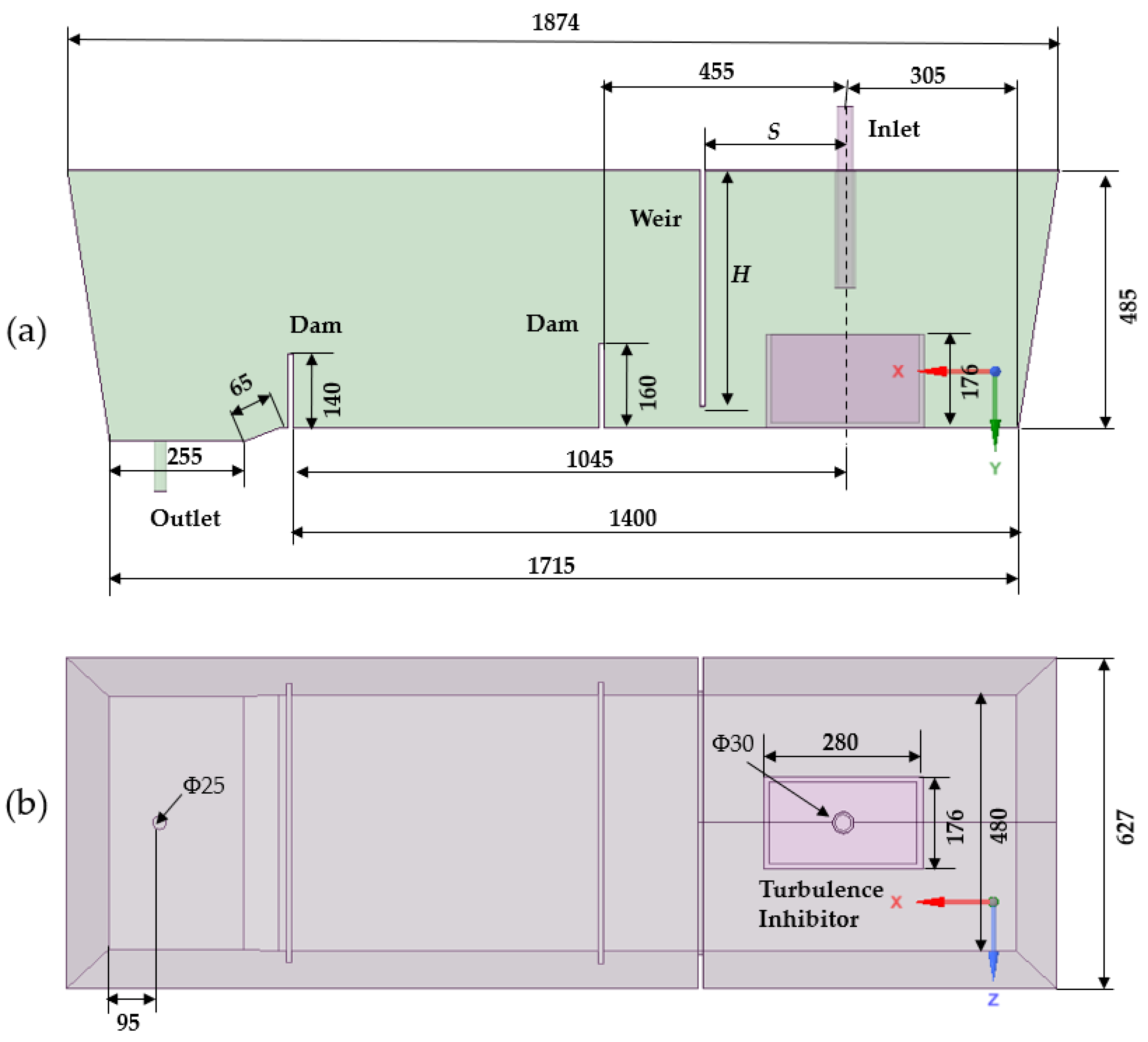
The normal casting speed in the steel plant is 1.5 m/min. The water model of the single-strand tundish was built based on similarity principles. The water model was constructed of plexiglass with the geometric scale ratio λ of 1:2.5. Figure 3 exhibits the geometric dimension of the water model furnished with one weir, two dams and one turbulence inhibitor. Dynamic similarity is determined by requiring the Froude number in the water model, which is equivalent to that in the prototype, as shown in Equation (17).

(Fr)_m = (Fr)_p

(17)

where m stands for water model and p is the prototype of the tundish. The Froude number Fr is defined as Equation (18)

Fr = u²/gL

(18)

Then, liquid velocity, volumetric flow rate and time ratio between the model and the prototype are described as a function of geometric scale ratio, as expressed in Equations (19)–(21). Parameters of the water model are obtained by these equations, which are listed in

Table 2. Process parameters of prototype and water model of the tundish.

Parameters	Prototype	Model
Liquid level (m)	1.063	0.425
Volume (m3)	6.109	0.391
Flow rate (m3/h)	20.7	2.1

.

$$\frac{u_m}{u_p}={(\frac{L_m}{L_p})}^{\frac{1}{2}}={\lambda }^{0.5}$$

(19)

$$\frac{Q_m}{Q_p}=\frac{u_m{L}_m{}^2}{u_p{L}_p{}^2}={\lambda }^{2.5}$$

(20)

$$\frac{{\tau }_m}{{\tau }_p}=\frac{L_m/u_m}{L_p/u_p}={\lambda }^{0.5}$$

(21)

The water model experiment was performed to consider the dispersion of tracer concentration. Once the water reaches the assumed liquid level (425 mm) and was stabilized, 200 mL saturated NaCl solution was used as the tracer injecting through the tundish inlet in 2 s. The detectors were placed below the weir and at the tundish outlet to record the tracer concentration. The pulse stimulus–response technique was applied to measure RTD. Afterwards, the time and the concentration were transformed to a dimensionless value in order to compare the flow characteristics obtained.

2.2.2. Inclusion Separation

The non-metallic inclusions (e.g., oxides Al₂O₃) are lighter than liquid steel. Thus, they have the tendency to float towards the surface of the liquid steel. The floating velocity of inclusion particles in the tundish can be modelled by Stoke’s law, described by Equation (22). Direct measurement on the separation of buoyant particles in the water model was performed to study the flotation of non-metallic inclusions in the tundish [36].

$$u_{\mathrm{s}}=\frac{\left({\rho }_{\mathrm{l}}-{\rho }_{\mathrm{s}}\right)\mathrm{g}{d}_{\mathrm{s}}^2}{18\mu }$$

(22)

where, u_s is the inclusion floating velocity, ρ_l is the density of liquid steel, ρ_s is the density of inclusion, g is the gravity acceleration, d_s is the solid inclusion diameter, μ is viscosity of liquid steel.

To satisfy the similarity of inclusion floating behavior, it is necessary that particles trajectories should be similar to the inclusions in molten steel. The particle diameter in the water model can be evaluated based on Equation (23), which is derived from Equations (19) and (22).

$$d_{\mathrm{s},\mathrm{m}}^2=\frac{u_{\mathrm{s},\mathrm{m}}}{u_{\mathrm{s},\mathrm{m}}}\cdot \frac{{\mu }_{\mathrm{m}}}{{\mu }_{\mathrm{p}}}\cdot \frac{\left({\rho }_{\mathrm{l},\mathrm{p}}-{\rho }_{\mathrm{s},\mathrm{p}}\right)}{\left({\rho }_{\mathrm{l},\mathrm{m}}-{\rho }_{\mathrm{s},\mathrm{m}}\right)}\cdot d_{\mathrm{s},\mathrm{p}}^2={\lambda }^{0.5}\cdot \frac{{\mu }_{\mathrm{m}}}{{\mu }_{\mathrm{p}}}\cdot \frac{\left({\rho }_{\mathrm{l},\mathrm{p}}-{\rho }_{\mathrm{s},\mathrm{p}}\right)}{\left({\rho }_{\mathrm{l},\mathrm{m}}-{\rho }_{\mathrm{s},\mathrm{m}}\right)}\cdot d_{\mathrm{s},\mathrm{p}}^2$$

(23)

By applying constants listed in

Table 3. Input parameters and boundary conditions used for computational fluid dynamics (CFD) simulations and water model.

Parameter	Value
Steel density	7080 kg/m3
Water density	998 kg/m3
Steel viscosity	0.0064 Pa·s
Water viscosity	0.001 Pa·s
Reference Pressure	101,325 Pa
Inclusion density	2700 kg/m3
Particle density (water model)	800 kg/m3
Outlet (outflow ratio)	1
Wall	No slip
Surface of inlet tank (flow)	Free slip
Surface of outlet tank (flow)	Free slip
Surface of inlet tank (inclusion)	50% escape
Surface of outlet tank (inclusion)	100% escape
Tracer inlet (E-curve)	1 (t ≤ 0–2 s), 0 (t > 2 s)

, the relation of particle diameters between the modelled particles and the real inclusions is expressed as:

$$d_{\mathrm{s},\mathrm{m}}^2=2.184\cdot d_{\mathrm{s},\mathrm{p}}^2$$

(24)

Drift beads were used to model the inclusions in water experiment. The particles were obtained by sieving with three size distribution ranges: 124–150 μm, 89–124 μm, and 74–89 μm. They represent the inclusions diameter of 84–101 μm, 60–84 μm and 50–60 μm in liquid steel, respectively. In total four grams’ spherical particles were added through the inlet pipe. The particles collected from the outlet were weighted with a Sartorius electrobalance after drying. The inclusion removal rate is calculated by Equation (25).

$$\eta =\frac{W_{\mathrm{in}}-W_{\mathrm{out}}}{W_{\mathrm{in}}}\times 100\%$$

(25)

2.3. Computational Fluid Dynamics (CFD) Model

CFD software STAR-CCM + V.13 (Siemens PLM software, Plano, TX, USA) was performed to simulate the fluid flow, the inclusion removal, and the residence-time distribution [37]. The assumptions made for the mathematical model are described below:

• The model is based on a 3D standard set of the Navier–Stokes equations.
• Isothermal and steady-state liquid flow is considered.
• The motion of inclusions is simulated by solving the force balance equations.
• The realizable k-ε model is used to describe the turbulence.
• The free surface is flat and is kept at a fixed level. The tundish slag layer is not included.
• The surface tension and wettability at slag/steel/inclusion interphase boundaries are not included.

2.3.1. Transport Equation

The molten steel flow is defined as a three-dimensional flow with constant density. Equations (26) and (27) are the governing equations used to describe the continuous phase [38].

Continuity:

$$\frac{\partial \left(\rho u_j\right)}{\partial x_j}=0$$

(26)

Momentum:

$$\rho u_j\frac{\partial u_i}{\partial x_j}=-\frac{\partial P}{\partial x_i}+\frac{\partial }{\partial x_j}\left[\left(\mu +{\mu }_t\right)\left\{\frac{\partial u_i}{\partial x_j}+\frac{\partial u_j}{\partial x_i}\right\}\right]+\rho g_i+S_F$$

(27)

Realizable k-ε model:

$$\frac{\partial }{\partial t}\left(\rho k\right)+\frac{\partial }{\partial x_j}\left(\rho k{u}_j\right)=\frac{\partial }{\partial x_j}\left[\left(\mu +\frac{{\mu }_t}{{\sigma }_k}\right)\frac{\partial k}{\partial x_j}\right]+G_k+G_b-\rho \epsilon -Y_M+S_k$$

(28)

$$\frac{\partial }{\partial t}\left(\rho \epsilon \right)+\frac{\partial }{\partial x_j}\left(\rho \epsilon u_j\right)=\frac{\partial }{\partial x_j}\left[\left(\mu +\frac{{\mu }_t}{{\sigma }_{\epsilon }}\right)\frac{\partial \epsilon }{\partial x_j}\right]+\rho C_{1}S\epsilon -\rho C_2\frac{{\epsilon }^2}{k+\sqrt{v\epsilon }}+C_{1\epsilon }\frac{\epsilon }{k}{C}_3{G}_b+S_{\epsilon }$$

(29)

where k is the turbulent kinetic energy; ε is the turbulent energy dissipation rate; µ is the molecular viscosity; µ_t is the turbulent viscosity; G_k represents the generation of turbulent kinetic energy due to the mean velocity; Y_M symbolizes the contribution of the fluctuating dilatation in compressible turbulence to the overall dissipation rate; υ is the kinematic viscosity; and σ_k and σ_ε are the turbulent Prandtl numbers for k and ε, respectively.

The success of numerical prediction methods depends to a great extent on the performance of the turbulence model used. The realizable k-ε model is substantially better than the standard k-ε model for many applications, including (i) round jets; (ii) boundary layers under strong adverse pressure gradients or separation; (iii) rotation and recirculation; and (iv) strong streamline curvature [39].

The Eulerian–Lagrangian approach has been applied to investigate the behavior of the non-metallic inclusions in the system. A one-way coupling approach is considered, where the influence of the micro-inclusion on the molten steel flow is neglected. The transport of the dispersed phase is predicted by tracking the trajectories of a certain number of representative parcels. The transport equation for each inclusion particle is given as [37]:

$$m_{\mathrm{i}}\frac{d{V}_{\mathrm{p}}}{\partial t}=F_{\mathrm{d}}+F_{\mathrm{p}}+F_{\mathrm{vm}}+F_{\mathrm{g}}+F_{\mathrm{l}}+F_{\mathrm{td}}$$

(30)

where m_i and V_p stand for the mass and the velocity of the particle. On the right side of Equation (30), the particle–fluid interaction forces are drag force (F_d), pressure gradient force (F_p), virtual mass forces (F_vm), gravitational force (F_g), lift force (F_l) and turbulent dispersion (F_td), respectively.

To calculate the residence-time distribution (RTD), the transport of a passive scalar is simulated by solving a filtered advection-diffusion equation. The passive scalar transport equation is solved at each time step once the fluid field is calculated.

$$\rho \frac{\partial \overline{C}}{\partial t}+\rho \overline{u_j}\frac{\partial \overline{C}}{\partial x_j}-\frac{\partial }{\partial x_j}\left[D_{eff}\frac{\partial \overline{C}}{\partial x_j}\right]=0$$

(31)

where D_eff is the effective diffusivity. The velocity field is solved obtained from a steady-state simulation and remained constant during the calculation of the passive scalar.

2.3.2. Mesh and Boundary Conditions

The volume mesh was generated in Star-CCM + V13.04 using the trimmer and prism layer meshing options. Three prism layers were generated next to all the walls. The surface mesh was generated first. Then the volume mesh was built based on the surface mesh by adjusting the growth rate and the biggest mesh size. A base mesh size of 0.006 m was used in this study. The surface average y + value in the first layer of the mesh near the wall is 2. A half tundish model was simulated through its symmetry plane in order to save time on CFD calculations. The final CFD model possesses a total of 3.6 million trimmer cells in the computing domain.

No-slip conditions were applied on all solid surfaces for the liquid steel phase. A constant inlet velocity was used. At the outlet of tundish, the outflow boundary condition was applied. A wall function was used to bridge the viscous sub-layer and to provide the near-wall boundary conditions for the average flow and the turbulence transport equations.

In the calculation, a discrete random walk model was applied to simulate the inclusion trajectories. To simplify the model, the inclusion particles were assumed to have a spherical shape. Agglomeration and collision of the inclusion particles were not considered. Considering the strong mixing and high turbulence flow of the entering stream, inclusion particles that reach the top surface of the inlet tank were regarded as 50% removal and 50% rebound. Inclusion particles that reach the top surface of the outlet tank were regarded as 100% removal due to the low turbulence flow, while the rest were considered as rebound. In total, around 6500 inclusion particles were injected through the inlet. The inclusion particle (Al₂O₃) density was set as 2700 kg m⁻³. Input parameters are listed in Table 3.

Zero mass flux was applied at walls and free surface for the passive scalar equation. At t = 0–2 s the mass fraction of tracer at the inlet was set to be equal to 1. When t > 2 s it was given as zero. The concentration of the tracer at the outlet was monitored from t = 0 to 3000 s and the RTD curves were obtained from the numerical calculation.

2.3.3. Solution Procedure

The discretized equations were solved in a segregated manner with the semi-implicit method for the pressure-linked equations (SIMPLE) algorithm. The second-order upwind scheme was used to calculate the convective flux in the momentum equations. The solution was judged to be converged when the residuals of all flow variables were less than 1 × 10⁻⁴, together with the stability of the velocity and the turbulence at the key monitor points. The flow fields were calculated in steady state. The transient calculation was used to solve the discrete phase equations. The under-relaxation parameters of flow calculations for the pressure, the velocity and the turbulence were 0.3, 0.7 and 0.8, respectively.

3. Results

The use of weir and dam in the tundish can significantly reduce the short circuiting and by-passing. The high turbulence region can be confined in the inlet tank. However, a significant fraction of the tundish will act as a dead volume in the lee of the weir and dam [4]. Therefore, this study focused on the effect of the weir position on the flow patterns in the single-strand tundish. Two geometric factors, the distance between weir and inlet (S) and the depth of the weir (H), were investigated in the water model experiment and shown in Figure 3a.

The experiments were divided into two steps: (i) varying the distance between weir and inlet, to find an optimal position in the horizontal direction; (ii) varying the depth of weir to find an optimal position in the vertical direction, while the horizontal position of the weir was fixed based on the result of step (i).

3.1. Water Model

Five experimental cases were studied with different combinations of the two factors levels, listed in

Table 4. Five studied cases of tundish water model experiment.

Case	A1	A2	A3	B1	B2
S(mm)	265	315	365	265	265
H(mm)	360	360	360	330	390

. The experimental cases can be divided into two groups: (i) Cases A1, A2 and A3, varying location of the weir; (ii) Cases B1, A1 and B2, varying depth of the weir.

3.1.1. Effect of Distance between Weir and Inlet

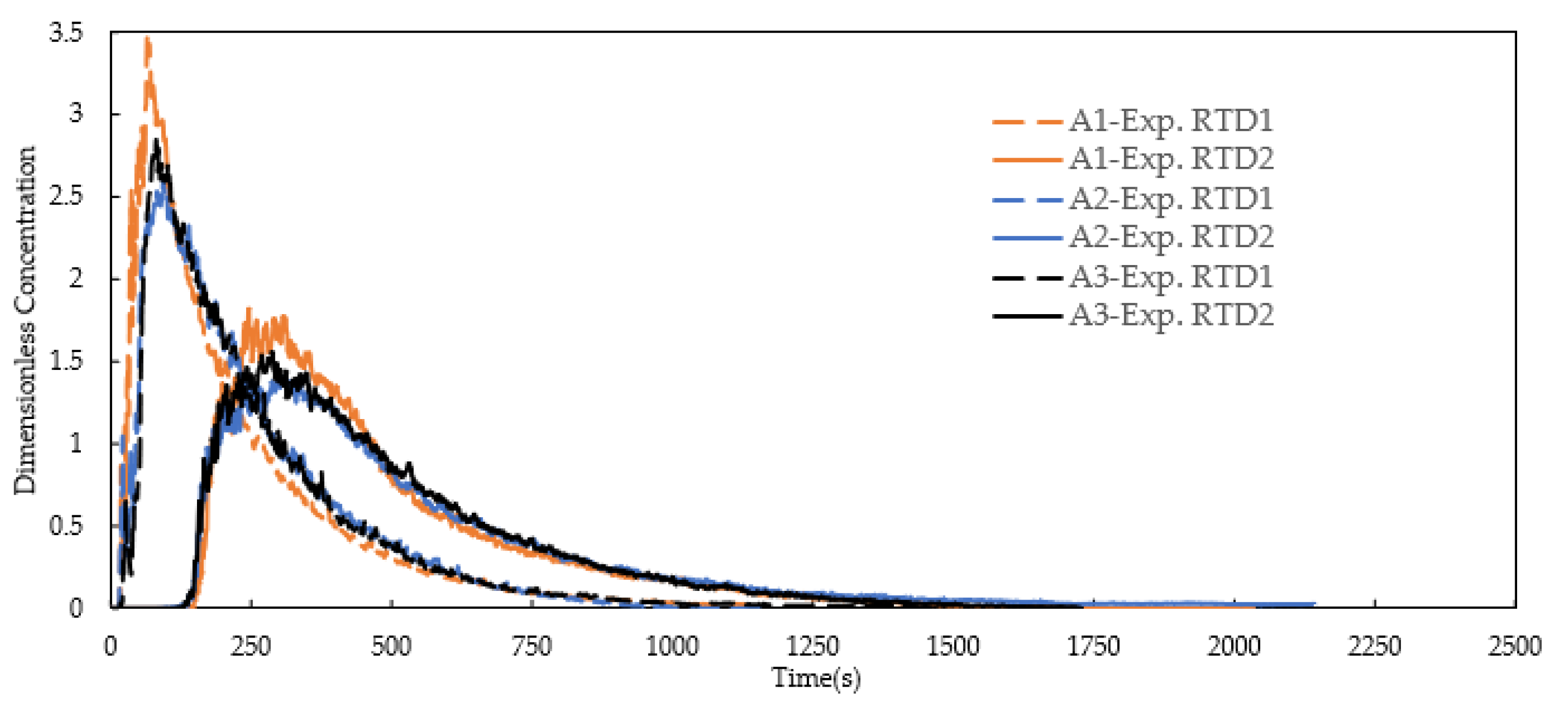
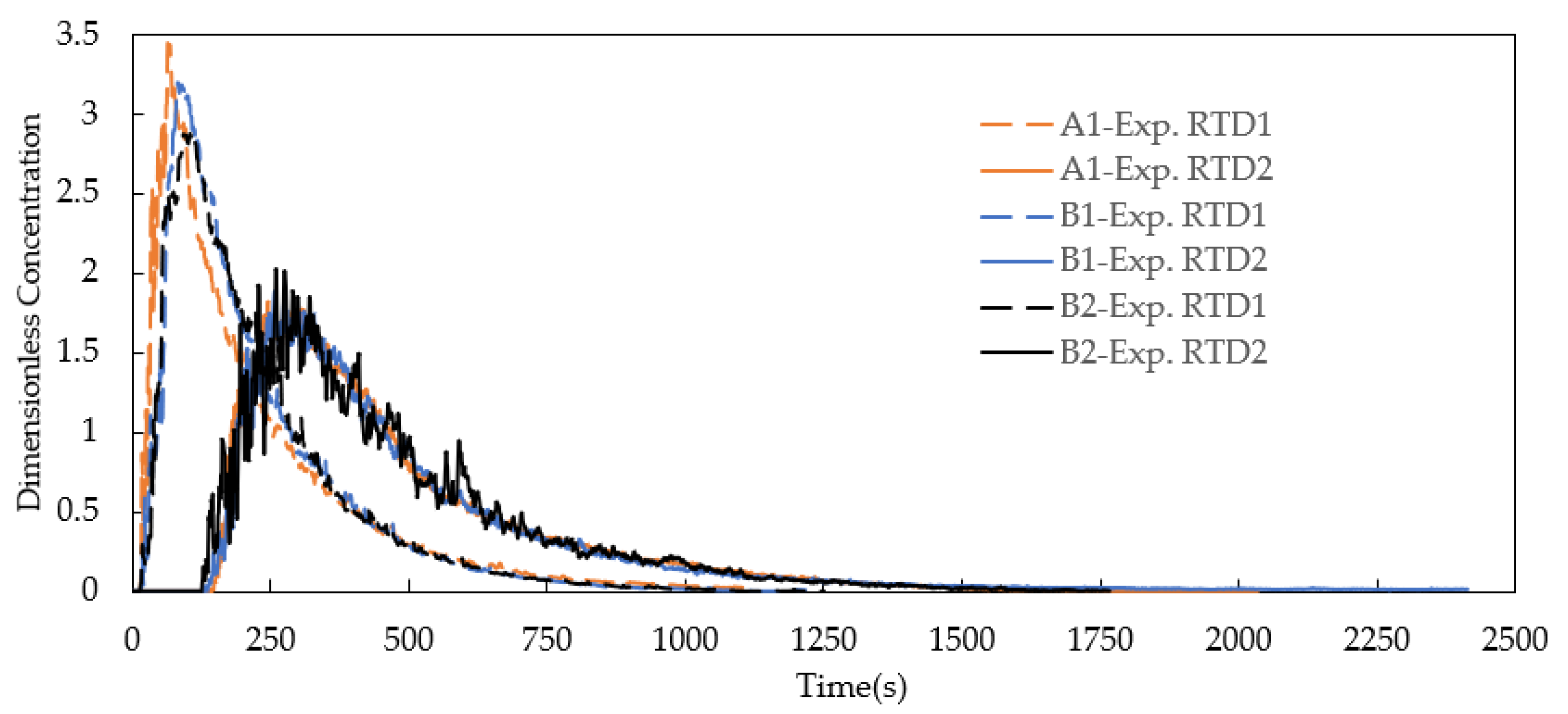
Figure 4 displays the measured RTD curves for Cases A1, A2 and A3. The experimental curves of inlet tank (RTD1) and entire tundish (RTD2) were measured below the weir and at the outlet of the tundish, respectively. RTD1 has a higher peak value compared with RTD2 for all the three cases. When comparing these cases, Case A1 gives the highest peak value of both RTD1 and RTD2 due to the shortest distance between the weir and inlet which results in the smallest volume of the inlet tank.

The analysis of RTD curves of Cases A1, A2 and A3 are shown in

Table 5. The water model experiment results of Cases A1, A2 and A3.

Case		A1 (S = 265 mm)	A2 (S = 315 mm)	A3 (S = 365 mm)
Inlet tank	Vp1/V1	0.048	0.078	0.082
	Vm1/V1	0.621	0.652	0.659
	Vd1/V1	0.331	0.270	0.259
Outlet tank Tundish	Vp2/V2	0.290	0.248	0.200
	Vm2/V2	0.413	0.494	0.484
	Vd2/V2	0.297	0.258	0.316
	Vp/V	0.215	0.186	0.161
	Vm/V	0.477	0.552	0.542
	Vd/V	0.308	0.262	0.293
	Mean(θ)	0.692	0.732	0.703

, including the data of volume fractions of plug flow, mixed flow and dead zone of inlet tank, outlet tank and entire tundish separately. The results convey that the inlet tank contains mostly the mixed flow (V_m1/V₁) while the volume fraction of plug flow (V_p1/V₁) is very small. Plug flow is mainly concentrated in the outlet tank. The volume fraction of plug flow in the outlet tank (V_p2/V₂) decreases with the increment of the distance between weir and inlet. Case A2 has the lowest dead volume fraction of the entire tundish (V_d/V).

The ratio between plug flow volume and mixed flow volume is listed in

Table 6. Ratio between mixed flow and plug flow and inclusion removal rate of Cases A1, A2 and A3.

Case		A1 (S = 265 mm)	A2 (S = 315 mm)	A3 (S = 365 mm)
Inlet tank (Vm1/Vp1)		12.90	8.33	8.04
Outlet tank (Vp2/Vm2)		0.70	0.50	0.41
Entire tundish (Vp/Vm)		0.45	0.34	0.30
η/%	84–101 (μm)	92.03	91.73	90.39
	60–84 (μm)	77.48	76.52	74.12
	50–60 (μm)	60.07	57.18	53.71

. Increasing the distance between weir and inlet, V_m1/V_p1 (the ratio of mixed flow volume to plug flow volume of the inlet tank) and V_p2/V_m2 (the ratio of plug flow volume to mixed flow volume of outlet tank) decreases gradually. V_p/V_m (the ratio of plug flow volume to mixed flow volume of entire tundish) decreases as well. These values were applied to assess the inclusion removal rate. The floating beads were collected from the outlet of the tundish after drying and weighing. Table 6 gives the measured inclusion removal rate of three different size ranges of inclusions (84–101 μm, 60–84 μm and 50–60 μm), calculated by Equation (25).

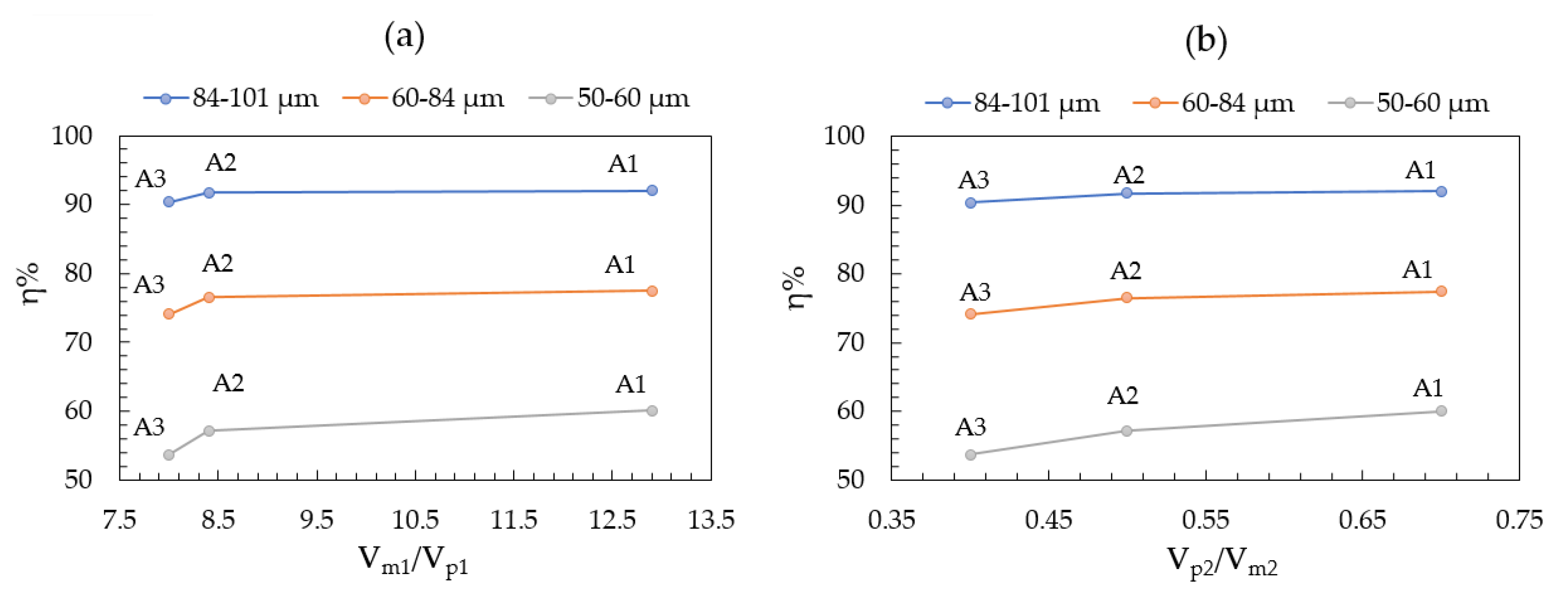
Figure 5 displays the relationship between V_m1/V_p1 in the inlet tank, V_p2/V_m2 in the outlet tank and inclusion removal rate for Cases A1, A2 and A3. Both V_m1/V_p1 (inlet tank) and V_p2/V_m2 (outlet tank) show the behavior of “larger-is-better” with regard to the inclusion removal rate. The larger ratio of V_m1/V_p1 in the inlet tank means an effective release of turbulent kinetic energy of the entering flow, leading to a stable flow in the outlet tank. Consequently, the larger ratio of V_p2/V_m2 in the outlet tank increases the inclusion floatation removal due to the stable horizontal flow pattern near the steel/slag interface. The optimized distance between weir and inlet is 265 mm (Case A1). The removal of small inclusions is more sensitive to the variation of weir location than that of big inclusions, for example, the removal of small inclusions (50–60 μm) in Case A1 is 6.4% higher than that in Case A3. The removal of big inclusions (84–101 μm) in Case A1 is only 1.6% higher than that in Case A3.

3.1.2. Effect of Height of Weir

Figure 6 illustrates the measured RTD curves for Cases A1, B1 and B2 (variation of depth of weir). The breakthrough time of RTD curves is quite similar. Case A1 shows the highest peak value of the three RTD1 curves. The RTD curves of the entire tundish (RTD2) for the three cases are quite similar. Case B2 displays a high fluctuation of RTD2, which might be caused by the increased local turbulence flow when the depth of the weir increases.

The experimental data of measured RTD curves and inclusion removal of Cases A1, B1 and B2 are listed in

Table 7. Water model experiment results of Cases B1, A1 and B2.

Case		B1 (H = 330 mm)	A1 (H = 360 mm)	B2 (H = 390 mm)
Inlet Tank	Vp1/V1	0.087	0.048	0.082
	Vm1/V1	0.672	0.621	0.691
	Vd1/V1	0.241	0.331	0.227
Outlet Tank	Vp2/V2	0.258	0.290	0.249
	Vm2/V2	0.413	0.413	0.445
	Vd2/V2	0.330	0.297	0.307
Entire Tundish	Vp/V	0.208	0.215	0.200
	Vm/V	0.488	0.477	0.516
	Vd/V	0.304	0.308	0.284
	Mean(θ)	0.696	0.692	0.716

, including the data of volume fractions of plug flow, mixed flow and dead zone of inlet tank, outlet tank and entire tundish separately. It is found that the dimensionless mean residence time first slightly decreases and then increases, varying the depth of weir from 330 mm to 390 mm. The volume fraction of dead zone in the entire tundish is 30.4% (Case B1), 30.8% (Case A1) and 28.4% (Case B2), respectively. The values of V_d/V of Cases B1 and A1 are quite close to each other, therefore, it is difficult to compare them if only based on a criterion of dead volume fraction.

Applying the tanks-in-series model, the RTDs in inlet tank and outlet tank were analyzed separately (

Table 8. Ratio between mixed flow and plug flow and inclusion removal rate of Cases B1, A1 and B2.

Case		B1 (H = 330 mm)	A1 (H = 360 mm)	B2 (H = 390 mm)
Inlet tank (Vm1/Vp1)		7.72	12.90	8.43
Outlet tank (Vp2/Vm2)		0.62	0.70	0.56
Entire tundish (Vp/Vm)		0.43	0.45	0.39
η/%	84–101 (μm)	90.03	92.03	91.24
	60–84 (μm)	73.25	77.48	75.69
	50–60 (μm)	55.16	60.07	57.26

). As the height of weir increases, V_m1/V_p1 increases from 7.72 to 12.90, then decreases to 8.43, while V_p2/V_m2 increases from 0.62 to 0.70, then decreases to 0.56. This indicates that Case A1 gives the best performance of the inclusion remove rate by using the criteria: “larger-is-better” for V_m1/V_p1 and V_p2/V_m2. Compared with Table 6, it indicates that the variation of weir location has a more significant effect on inclusion removal rate than the variation of height of weir, especially for the small inclusions (50–60 μm).

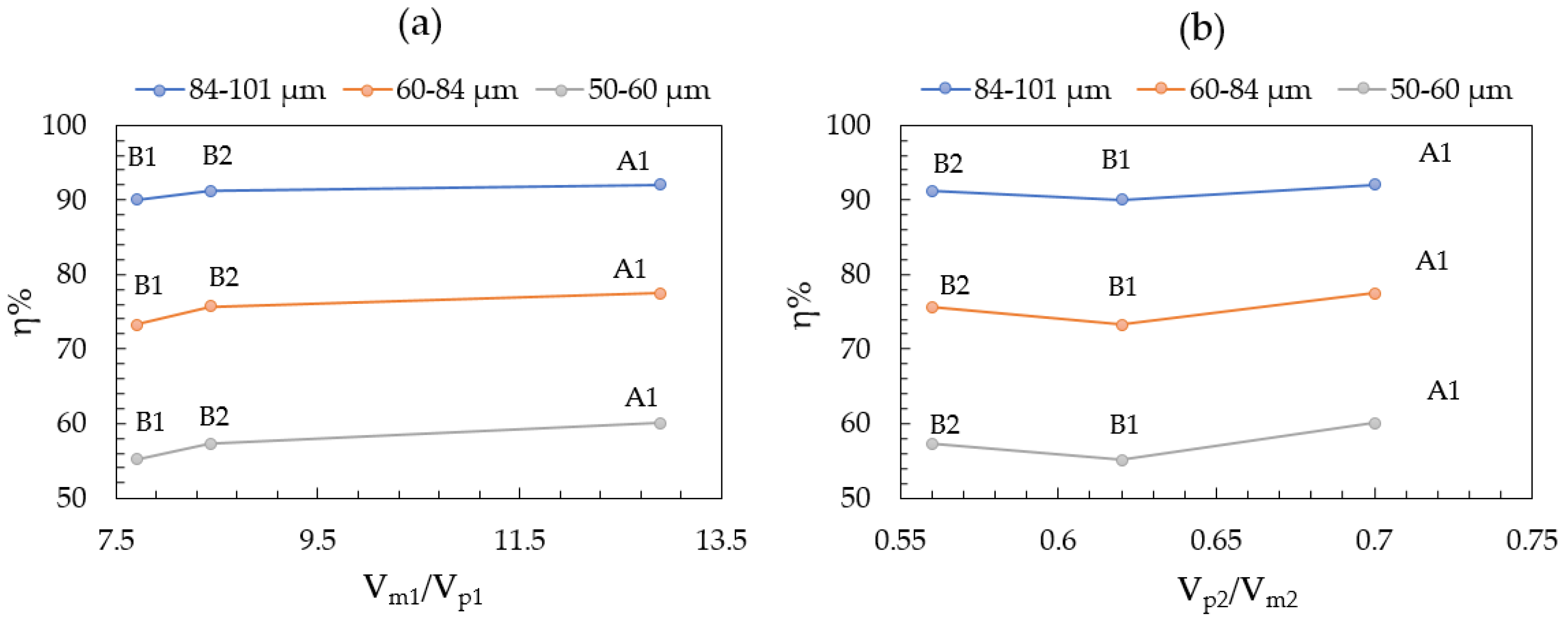
Table 8 lists the inclusion removal rate for Cases B1, A1 and B2 (variation of depth of weir) with three different size ranges of inclusions (84–101 μm, 60–84 μm and 50–60 μm). Figure 7a exhibits the relationship between V_m1/V_p1 (inlet tank) and inclusion removal rate for Cases B1, A1 and B2. V_m1/V_p1 (inlet tank) show the behavior of “larger-is-better” with regard to the inclusion removal rate. This result is consistent with result in the previous section.

However, it can be seen from Figure 7b that the inclusion removal rate slightly decreases with the increase of V_p2/V_m2 (outlet tank) for Cases B1 and B2. This is mainly due to the fact that Cases B1 and B2 have similar plug flow volume fractions (V_p2/V₂) in the outlet tank, which are 0.258 and 0.249 respectively. Therefore, dead volume fraction (V_d2/V₂) has a more obvious effect on inclusion removal under such condition. V_d2/V₂ of Cases B1 and B2 are 0.330 and 0.307, indicating better inclusion removal rate for Case B2. Similarly, the removal of small inclusions (50–60 μm) is more sensitive to the variation of height of the weir in comparison with the removal of big inclusions (84–101 μm).

3.2. Theoretical Model

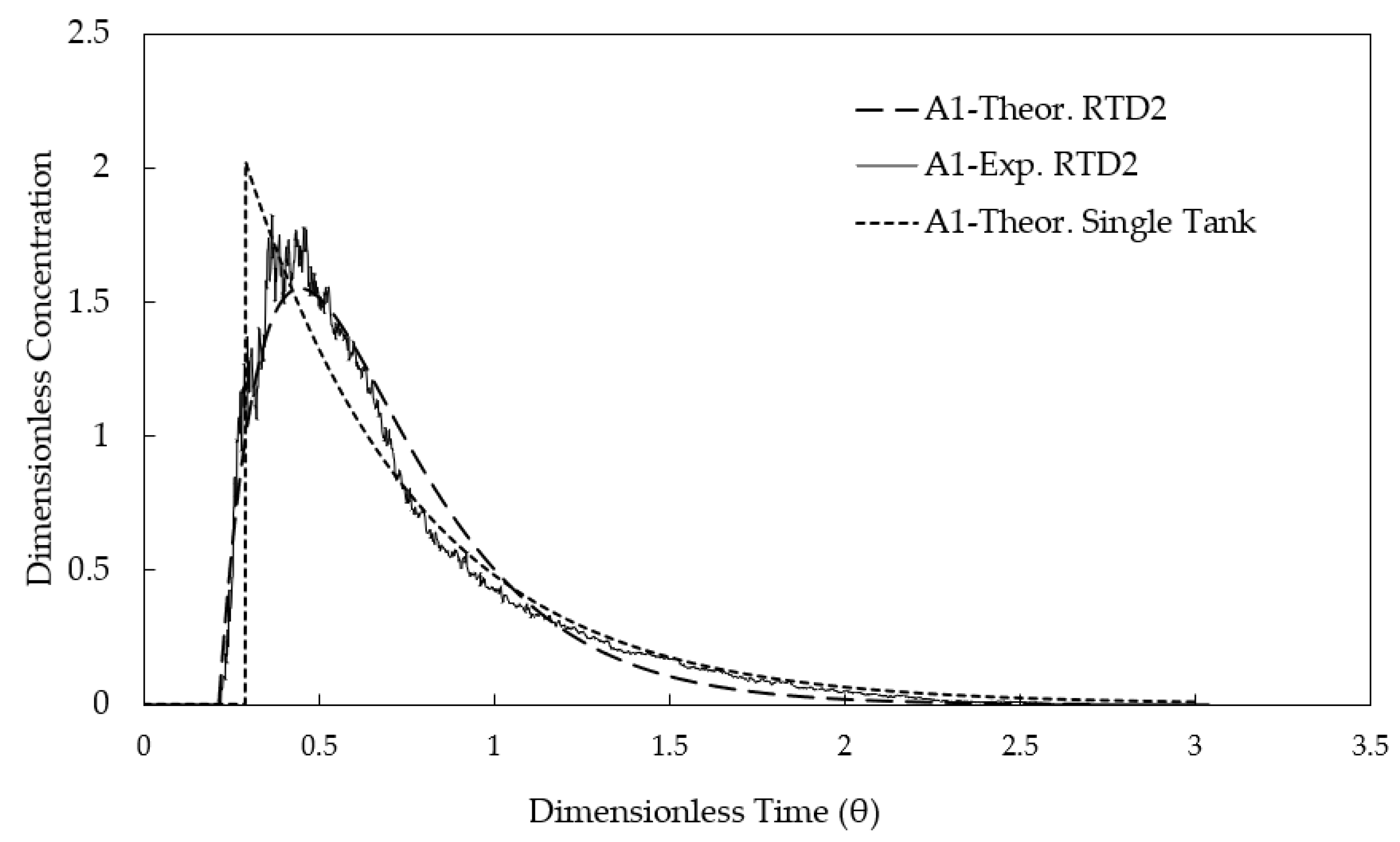
Figure 8 shows the comparison of experimental RTD curve and theoretical calculated RTD curves by using the single-tank model given by Equation (5) and tanks-in-series model given by Equation (16). It is obvious that the tanks-in-series model provides a better fitting function compared with single-tank model, indicating that the derived Equation (16) is suitable to describe the RTD curve of the entire tundish.

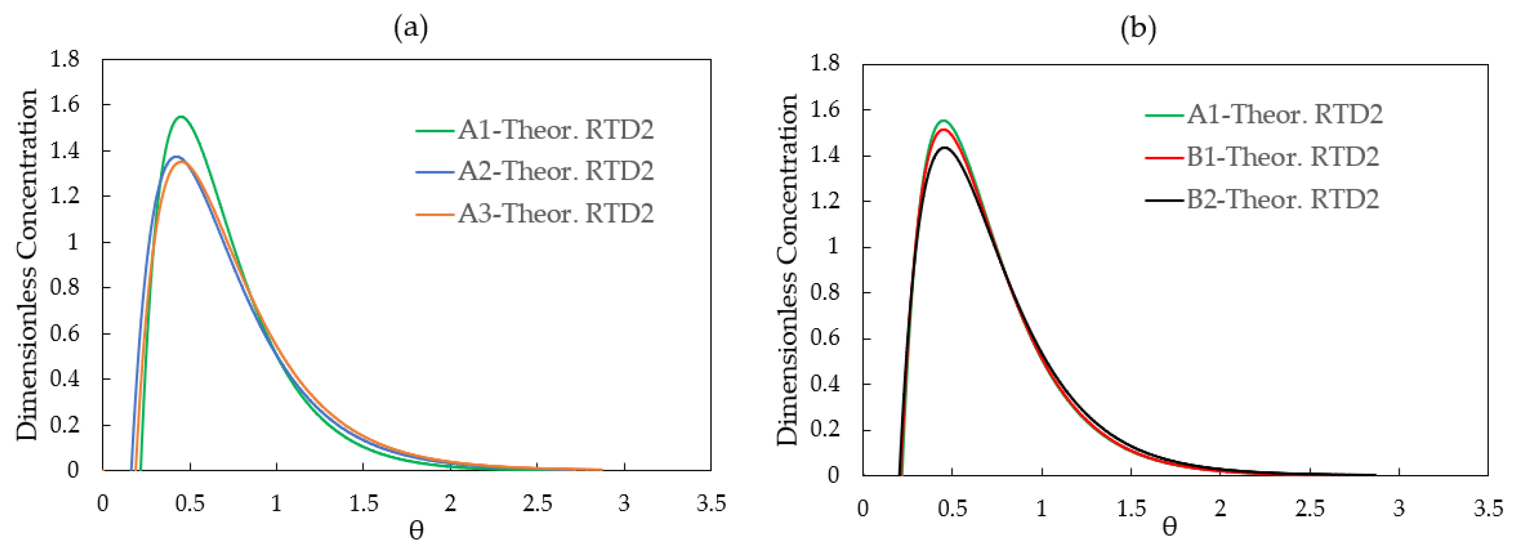
Figure 9 displays the theoretical fitted curves for the two experimental groups with geometric variation on the weir location and the height of the weir: (1) Cases A1, A2 and A3 for weir location; (2) Cases B1, A1 and B2 for weir height. They are in good agreement with measured RTD curves in Figure 4 and Figure 6. The difference between the compared cases becomes more visible because the fluctuation of the measured data was filtered out. As indicated in Figure 9a, the three cases have a difference in the breakthrough time and peak time, which indicates the difference in plug flow in the tundish due to variation of the weir location. Case A1 shows the largest value of the peak time. In group 2 (Cases B1, B2 and A1), the three cases have almost the same breakthrough time and peak time, indicating that the depth of the weir has a minor effect on plug flow volume fraction in the tundish.

3.3. CFD Model

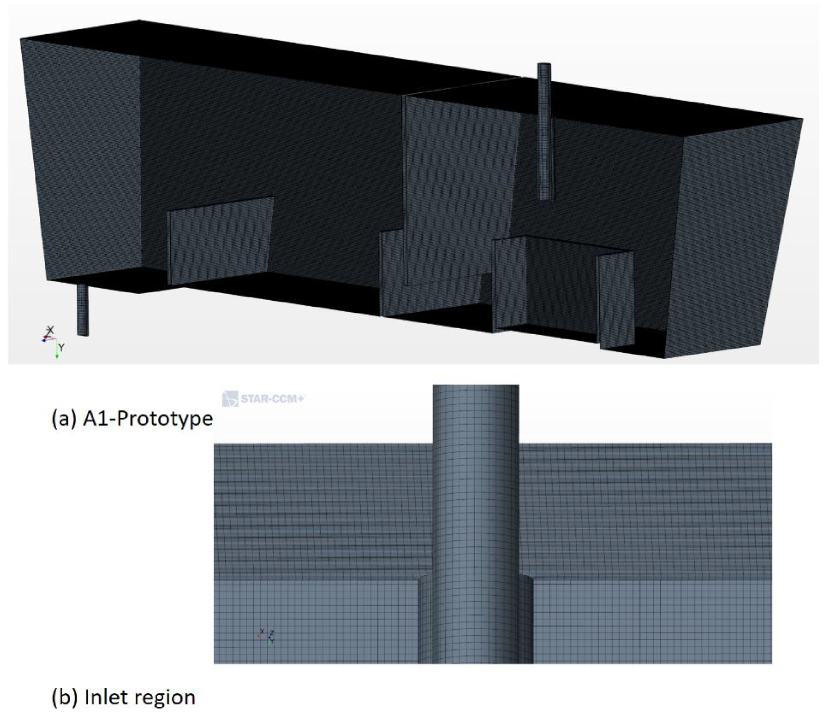
The purpose of the CFD modelling was to confirm the conclusion drawn from water model experiments and theoretical analysis. Two selected CFD simulation cases, A1-prototype and A3-prototype, were created for the simulation of the full-scale tundish. The selection of cases is based on the observation of experimental data and theoretical analysis that the variation of distance between weir and inlet has a significant effect on the volume of different flow patterns. The plant operating conditions of tundish (listed in Table 2 and Table 3) were applied to simulate the liquid steel flow, RTD and inclusion removal rate. Figure 10 shows the trimmer CFD mesh in the computing domain of the tundish (Figure 10a) and near the inlet region (Figure 10b, zoom-in view). The validation of the tundish CFD model including mesh dependency study (RTD and inclusions) and comparison with the experimental data (RTD) can be found in previous works [40,41].

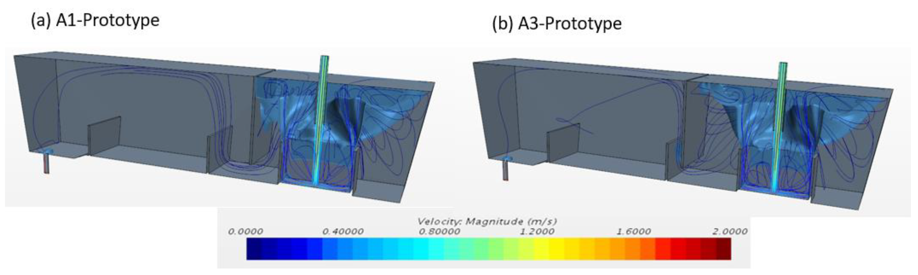
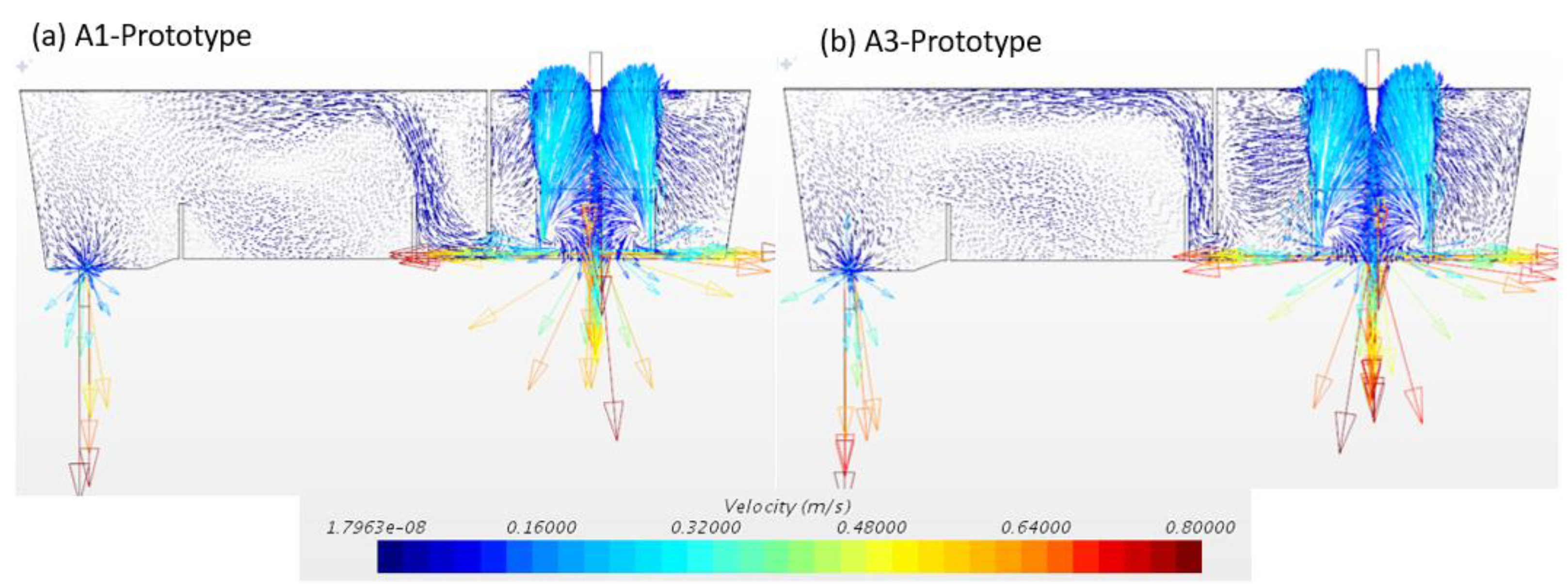
Figure 11 displays the predicated three-dimensional isosurface of turbulent kinetic energy (k = 0.00045 J/kg) and flow streamlines through CFD modelling. Figure 12 displays the predicated velocity in the central plane of the tundish. The weir reveals the function of confining the turbulence flow within the inlet tank. In the outlet tank, the plug flow provides favorable conditions for the inclusion removal. The Case A1-prototype gives a larger volume fraction of high turbulence region in the inlet tank which indicates a strong mixed flow. The dam reorients the flow after the weir in the outlet tank. The combination of weir and dam in the Case A1-prototype can form a suitable release angle for the main stream of liquid steel. For the Case A3-prototype, the short distance between weir and dam drives the liquid steel flows upwards, leading to a rapid increase in vertical momentum and a decrease in horizontal momentum in the outlet tank. The Case A1-prototype shows a larger zone with high horizontal velocities near the top surface in the outlet tank, which creates a better opportunity for inclusion removal.

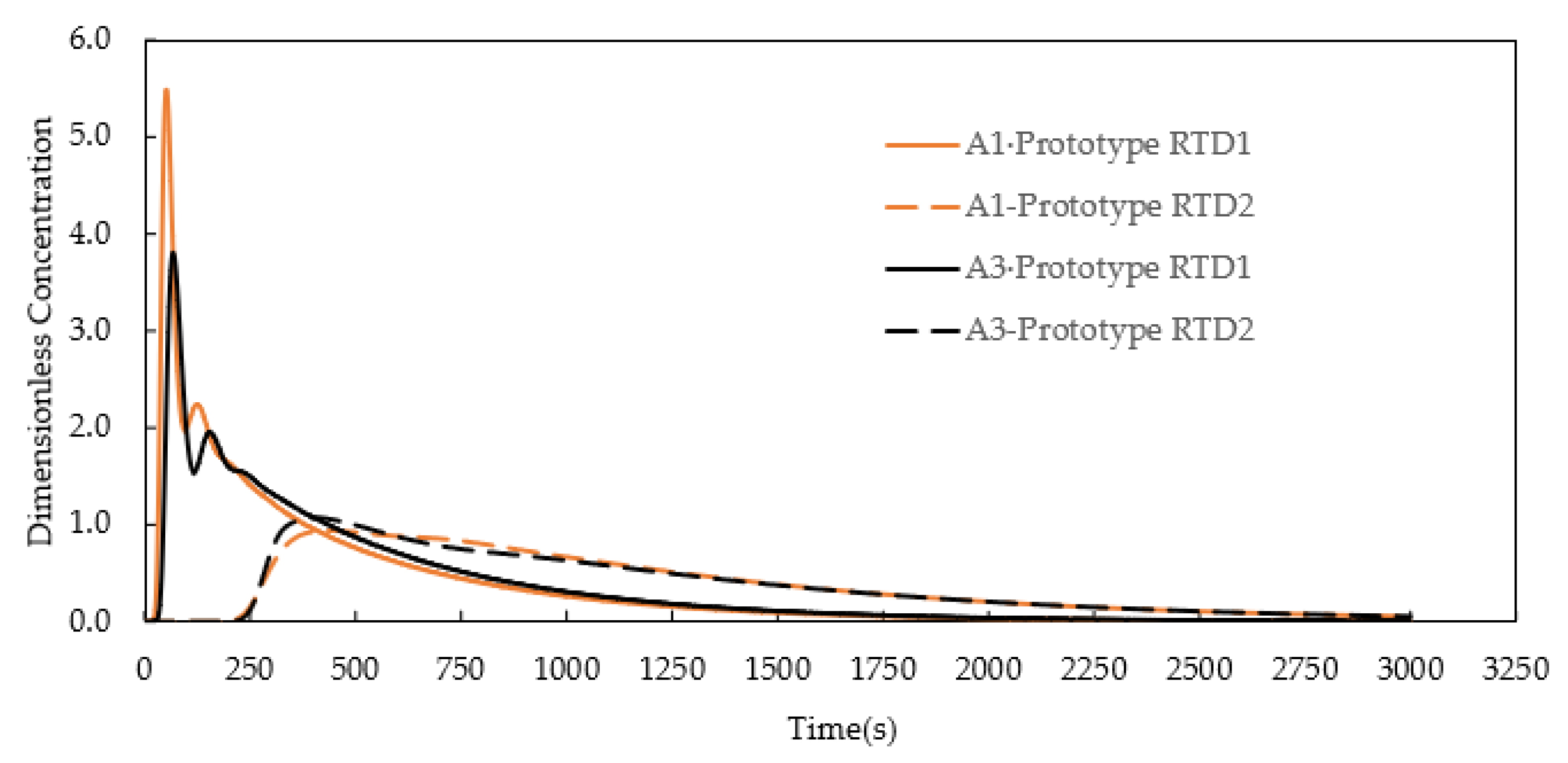
Figure 13 exhibits the calculated RTD curves by CFD modelling for the Cases A1-prototype and A3-prototype with different weir locations. The calculated RTD1curves were obtained below the weir by using the average value on a plane. RTD2 were obtained at the outlet of the tundish. RTD1 has a higher concentration peak comparing with RTD2 for both cases. The Case A1-prototype displays the higher peak value in RTD1 curves due to a shorter distance between weir and inlet. The RTD curves imply the non-ideal behavior of liquid steel flow in the tundish.

The data analysis of calculated RTD curves by CFD modelling are presented in

Table 9. Data analysis of RTD curves in real tundish (CFD prediction).

Case	Variable	A1-Prototype (S = 662 mm)	A3-Prototype (S = 912 mm)
Inlet tank	Vp1/V1	0.11	0.13
	Vm1/V1	0.58	0.62
	Vd1/V1	0.31	0.25
Outlet tank	Vp2/V2	0.38	0.36
	Vm2/V2	0.55	0.54
	Vd2/V2	0.07	0.10
Tundish	Vp/V	0.30	0.28
	Vm/V	0.56	0.57
	Vd/V	0.14	0.15
	Mean(t), second	959	948

. In the inlet tank, it contains mostly mixed flow. The values of V_m1/V₁ are 58% for the Case A1-prototype and 62% for Case A3-prototype. The volume fraction of plug flow is small (V_p1/V₁). The dead volume fractions in the inlet tank of the two cases are high, 31% and 25% respectively. This means that further design improvement of the inlet tank can enhance the tundish performance, for instance, and optimize inlet nozzle and turbulence inhibitor. Plug flow is concentrated in the outlet tank. The volume fraction of plug flow in the outlet tank (V_p2/V₂) slightly decreases from 38% to 36% when increasing the distance between weir and inlet. For the entire tundish analysis, the Case A1-prototype shows a slightly lower dead volume fraction and a higher plug flow volume fraction when compared with the Case A3-prototype.

The RTD in the inlet tank and outlet tank were analyzed separately for the Cases A1-prototype and A3-prototype of the real tundish system. Increasing the distance between weir and inlet, V_m1/V_p1 decreases from 5.27 to 4.77 and V_p2/V_m2 decreases from 0.71 to 0.67, as listed in

Table 10. Ratio between mixed flow volume and plug flow volume and inclusion removal rate (CFD prediction).

Case		A1-Prototype	A3-Prototype
Inlet tank (Vm1/Vp1)		5.27	4.77
Outlet tank (Vp2/Vm2)		0.71	0.67
Entire tundish (Vp/Vm)		0.54	0.49
η/%	84–101 (μm)	90.09	88.65
	60–84 (μm)	77.66	73.92
	50–60 (μm)	72.34	66.89

. This indicates that Cases A1-prototype provides better performance when applying the criteria—“larger-is-better” for V_m1/V_p1 and V_p2/V_m2.

Table 10 presents the inclusion removal rates with different inclusion sizes for the Cases A1-prototype and A3-prototype. Three groups of inclusions were modelled (84–101 μm, 60–84 μm and 50–60 μm). The mean particle diameters of each group (92 μm, 72 μm and 55 μm) were used for the CFD modelling. Independent of the arrangement of weir position, the increase of inclusion size has more effect on the inclusion removal. For the Case A1-prototype, the inclusion removal rate ranges from 72% (50–60 µm) to 90% (84–101 µm). For Case A3-prototype, the inclusion removal rate ranges from 67% (50–60 µm) to 89% (84–101 µm). High removal of larger inclusions is mainly due to the buoyancy force, affected by the inertial forces from the liquid steel. The Case A1-prototype presents a better inclusion removal rate than the Case A3-prototype, especially for the inclusions with a size of 50–60 µm. The removal of small inclusions (50–60 µm) is more sensitive to the locations of the weir in comparison with the big inclusions (84–101 μm).

In Table 10, the relationship between V_m1/V_p1 (inlet tank), V_p2/V_m2 (outlet tank) and inclusion removal rate reveals the behavior of “larger-is-better”. This means that CFD modelling result can confirm the observation of water model experiments, which indicates that two interacting tanks in series model can be applied to reasonably predict the tundish performance in terms of inclusion removal rate.

4. Conclusions

A new tanks-in-series model for analyzing the non-ideal flow regimes in a single-strand tundish was proposed in this study. Water model experiment, theoretical model analysis and CFD model simulation were carried out to have a detailed investigation of inclusion removal in the tundish. The following conclusions can be drawn from the results:

• In the tanks-in-series model, the ratio between plug flow volume and mixed flow volume of divided tanks is proposed as a new criterion to evaluate the tundish performance related to inclusion removal rate. A strong mixed flow in the inlet tank promotes the mixing and inclusion collision growth. A strong plug flow in the outlet tanks promotes the floating removal of inclusions.
• The analysis of water model data shows that Case A1 (distance between weir and dam is 260 mm and depth of weir is 360 mm) gives the best performance of the tundish with regard to the inclusion removal rate. The variation of weir location has a more significant effect on the inclusion removal rate in comparison with the variation of height of weir, especially for the inclusions with a size of 50–60 µm.
• The derived equation using tanks-in-series model provides a better fitting function to the experimental data compared with the equation using the single-tank model. It indicates that the developed tanks-in-series model is suitable to describe the tundish flow patterns.
• The CFD modelling result confirms the observation of the water model experiments and theoretical analysis. The results can provide useful insight into the kinetics of inclusion flotation in tundish systems. The removal of relatively larger size inclusions from the tundish can be assessed qualitatively from the corresponding RTD curves of the tanks-in-series model.

Finally, it should be mentioned that the results from the water model experiment might not be scaled up to a full-scale tundish on a one-to-one basis. Therefore, the validation of the developed model by comparison with the corresponding plant trial data is highly desirable, for example the model validation by using tracer experiments on production heat. The transient behavior during ladle change and the flow patterns under non-isothermal conditions need to be considered in future work. If the model predications agree reasonably well with the plant trial data, there is a great potential to extend the application area of tanks-in-series model. For instance, to study the flow patterns of a multi-strand tundish, each outlet strand can be treated as a separate tank. The flow patterns in the multi-strand tundish can be investigated in the interconnected multiple tanks by using the proposed tanks-in-series model.

References

- MacMullin, R.B.; Weber, M. The theory of short-circuiting in continuous-flow mixing vessels in series and kinetics of chemical reactions in such systems. Trans. Am. Inst. Chem. Eng. 1935, 31, 409–458. [Google Scholar]
- Danckwerts, P.V. Continuous flow systems. Distribution of residence times. Chem. Eng. Sci. 1953, 2, 1–13. [Google Scholar] [CrossRef]
- Rodrigues, A.E. Residence time distribution (RTD) revisited. Chem. Eng. Sci. 2021, 230, 116188. [Google Scholar] [CrossRef] [PubMed]
- Szekely, J.; Ilegbusi, O.J. The Physical and Mathematical Modeling of Tundish Operations; Springer Science and Business Media LLC: New York, NY, USA, 1989. [Google Scholar]
- Mazumdar, D.; Guthrie, R.I.L. The Physical and Mathematical Modelling of Continuous Casting Tundish System. ISIJ Int. 1999, 39, 524–547. [Google Scholar] [CrossRef]
- Chattopadhyay, K.; Isac, M.; Guthrie, R.I.L. Physical and Mathematical Modelling of Steelmaking Tundish Operations: A Review of the Last Decade (1999–2009). ISIJ Int. 2010, 50, 331–348. [Google Scholar] [CrossRef] [Green Version]
- Kemeny, F.; Harris, D.J.; McLean, A.; Meadowcroft, T.R.; Young, D.J. Fluid flow studies in the tundish of a slab caster. In Proceedings of the 2nd Process Technol Conference on Continuous Casting of Steel, Chicago, IL, USA, 23–25 February 1981; pp. 232–245. [Google Scholar]
- Sahai, Y.; Ahuja, R. Fluid-flow and mixing of melt in steelmaking tundishes. Ironmak. Steelmak. 1986, 13, 241–247. [Google Scholar]
- Sahai, Y.; Emi, T. Melt flow characterization in continuous casting tundishes. ISIJ Int. 1996, 36, 667–672. [Google Scholar] [CrossRef]
- Sheng, D.Y. Design Optimization of a Single-Strand Tundish Based on CFD-Taguchi-Grey Relational Analysis Combined Method. Metals 2020, 10, 1539. [Google Scholar] [CrossRef]
- López-Ramírez, S.; Palafox-Ramos, J.; Morales, R.D.; Barrón-Meza, M.A.; Toledo, M.V. Effects of tundish size, tundish design and casting flow rate on fluid flow phenomena of liquid steel. Steel Res. 1998, 69, 423–428. [Google Scholar]
- Craig, K.J.; Kock, D.D.; Makgata, K.W.; Wet, G.J.D. Design Optimization of a Single-strand Continuous Caster Tundish Using Residence Time Distribution Data. ISIJ Int. 2001, 41, 1194–1200. [Google Scholar] [CrossRef]
- Jha, P.K.; Dash, S.K. Employment of different turbulence models to the design of optimum steel flows in a tundish. Int. J. Numer. Methods Heat Fluid Flow 2004, 14, 953–979. [Google Scholar] [CrossRef]
- Vargas-Zamora, A.; Palafox-Ramos, J.; Morales, R.D.; Díaz-Cruz, M.; Barreto-Sandoval, J.D.J. Inertial and buoyancy driven water flows under gas bubbling and thermal stratification conditions in a tundish model. Metall. Mater. Trans. B 2004, 35, 247–257. [Google Scholar] [CrossRef]
- Zhong, L.C.; Li, L.Y.; Wang, B.; Zhang, L.; Zhu, L.X.; Zhang, Q.F. Fluid flow behaviour in slab continuous casting tundish with different configurations of gas bubbling curtain. Ironmak. Steelmak. 2008, 35, 436–440. [Google Scholar] [CrossRef]
- Kumar, A.; Mazumdar, D.; Koria, S.C. Modeling of Fluid Flow and Residence Time Distribution in a Four-strand Tundish for Enhancing Inclusion Removal. ISIJ Int. 2008, 48, 38–47. [Google Scholar] [CrossRef] [Green Version]
- Bensouici, M.; Bellaouar, A.; Talbi, K. Numerical investigation of the fluid flow in continuous casting tundish using analysis of RTD curves. J. Iron Steel Res. Int. 2009, 16, 22–29. [Google Scholar] [CrossRef]
- Yang, S.; Zhang, L.; Li, J.; Peaslee, K. Structure Optimization of Horizontal Continuous Casting Tundishes Using Mathematical Modeling and Water Modeling. ISIJ Int. 2009, 49, 1551–1560. [Google Scholar] [CrossRef] [Green Version]
- Cwudziński, A. Numerical Simulation of Liquid Steel Flow in Wedge-type One-strand Slab Tundish with a Subflux Turbulence Controller and an Argon Injection System. Steel Res. Int. 2010, 81, 123–131. [Google Scholar] [CrossRef]
- Zheng, M.J.; Gu, H.Z.; Ao, H.; Zhang, H.X.; Deng, C.J. Numerical simulation and industrial practice of inclusion removal from molten steel by gas bottom blowing in continuous casting tundish. J. Min. Metall. Sec. B Metall. 2011, 47, 137–147. [Google Scholar]
- Tripathi, A. Numerical Investigation of Electro-Magnetic Flow Control Phenomenon in a Tundish. ISIJ Int. 2012, 52, 447–456. [Google Scholar] [CrossRef] [Green Version]
- Chen, D.F.; Xie, X.; Long, M.J.; Zhang, M.; Zhang, L.L.; Liao, Q. Hydraulics and mathematics simulation on the weir and gas curtain in tundish of ultrathick slab continuous casting. Metall. Mater. Trans. B 2014, 45, 392–398. [Google Scholar] [CrossRef]
- Chen, C.; Jonsson, L.T.I.; Tilliander, A.; Cheng, G.G.; Jönsson, P.G. A mathematical modeling study of tracer mixing in a continuous casting tundish. Metall. Mater. Trans. B 2015, 46, 169–190. [Google Scholar] [CrossRef]
- Chang, S.; Zhong, L.; Zou, Z. Simulation of flow and heat fields in a seven-strand tundish with gas curtain for molten steel continuous-casting. ISIJ Int. 2015, 55, 837–844. [Google Scholar] [CrossRef] [Green Version]
- Devi, S.; Singh, R.; Paul, A. Role of tundish argon diffuser in steelmaking tundish to improve inclusion flotation with CFD and water modelling studies. Int. J. Eng. Res. Technol. 2015, 4, 213–218. [Google Scholar]
- He, F.; Zhang, L.Y.; Xu, Q.Y. Optimization of flow control devices for a T-type five-strand billet caster tundish: Water modeling and numerical simulation. China Foundry 2016, 13, 166–175. [Google Scholar] [CrossRef]
- Neves, L.; Tavares, R.P. Analysis of the mathematical model of the gas bubbling curtain injection on the bottom and the walls of a continuous casting tundish. Ironmak. Steelmak. 2017, 44, 559–567. [Google Scholar] [CrossRef]
- Aguilar-Rodriguez, C.E.; Ramos-Banderas, J.A.; Torres-Alonso, E.; Solorio-Diaz, G.; Hernández-Bocanegra, C.A. Flow characterization and inclusions removal in a slab tundish equipped with bottom argon gas feeding. Metallurgist 2018, 61, 1055–1066. [Google Scholar] [CrossRef]
- Yang, B.; Lei, H.; Zhao, Y.; Xing, G.; Zhang, H. Quasi-symmetric transfer behavior in an asymmetric two-strand tundish with different turbulence inhibitor. Metals 2019, 9, 855. [Google Scholar] [CrossRef] [Green Version]
- Wang, Q.; Liu, Y.; Huang, A.; Yan, W.; Gu, H.; Li, G. CFD Investigation of effect of multi-hole ceramic filter on inclusion removal in a two-strand tundish. Metall. Mater. Trans. B 2020, 51, 276–292. [Google Scholar] [CrossRef]
- Tkadlečková, M.; Walek, J.; Michalek, K.; Huczala, T. Numerical Analysis of RTD Curves and Inclusions Removal in a Multi-Strand Asymmetric Tundish with Different Configuration of Impact Pad. Metals 2020, 10, 849. [Google Scholar] [CrossRef]
- Spalding, D.B. A note on mean residence-times in steady flows of arbitrary complexity. Chem. Eng. Sci. 1958, 9, 74–77. [Google Scholar] [CrossRef]
- Levenspiel, O. Tracer Technology: Modeling the Flow of Fluids; Springer-Verlag: New York, NY, USA, 2013. [Google Scholar]
- Levenspiel, O. Chemical Reaction Engineering, 3rd ed.; Wiley: New York, NY, USA, 1999; pp. 283–335. [Google Scholar]
- Ping, C. The Characterization and Evaluation of Fluid Flows in the Tundish of Steel Continuous Casting. PhD Thesis, The Northeastern University, Shenyang, China, 9 February 2015. [Google Scholar]
- Miki, Y.; Shimada, Y.; Thomas, B.G.; Denissov, A. Model of inclusion removal during RH degassing of steel. Iron Steelmak. 1997, 24, 31–38. [Google Scholar]
- Siemens, P.L.M. STAR-CCM + User Guide Version 13.04; Siemens PLM Software Inc: Munich, Germany, 2019. [Google Scholar]
- Patankar, S.V. Numerical Heat Transfer and Fluid Flow; Hemisphere Publishing Corporation: New York, NY, USA, 1980. [Google Scholar]
- Shih, T.H.; Liou, W.W.; Shabbir, A.; Yang, Z.; Zhu, J. A New k-ε eddy viscosity model for high reynolds number turbulent flows-model development and validation. Comput. Fluids 1994, 24, 227–238. [Google Scholar] [CrossRef]
- Sheng, D.Y.; Yue, Q. Modeling of Fluid Flow and Residence-Time Distribution in a Five-strand Tundish. Metals 2020, 10, 1084. [Google Scholar] [CrossRef]
- Sheng, D.Y. Mathematical Modelling of Multiphase Flow and Inclusion Behavior in a Single-Strand Tundish. Metals 2020, 10, 1213. [Google Scholar] [CrossRef]
Figure 1.
Residence-time distribution (RTD) function under three conditions of (a) plug flow, (b) mixed flow and (c) arbitrary flow.
Figure 2.
Theoretical models of tundish: (a) single-tank model; (b) tanks-in-series model; (c) schematic illustration.
Figure 3.
Geometry of water model: (a) front view (b) top view (unit: mm).
Figure 4.
Measured RTD curves of Cases A1, A2 and A3.
Figure 5.
The relationship between (a) Vm1/Vp1 in inlet tank and inclusion removal rate; (b) Vp2/Vm2 in outlet tank and inclusion removal rate for Cases A1, A2 and A3.
Figure 6.
Measured RTD curves of Cases A1, B1 and B2.
Figure 7.
The relationship between (a) Vm1/Vp1 in inlet tank and inclusion removal rate, and (b) Vp2/Vm2 in outlet tank and inclusion removal rate for Case B1, B2 and A1.
Figure 8.
Comparison of experimental and theoretical RTD curves in the entire tundish.
Figure 9.
Calculated RTD curves using tanks-in-series model (a) Group 1—variation of distance between weir and inlet (b) Group 2—variation of depth of weir.
Figure 10.
Computational domain and CFD mesh of single-strand tundish (a) A1-Prototype; (b) inlet region (zoom-in view).
Figure 11.
Calculated streamline and isosurface of turbulence kinetic energy (k = 0.0045 J kg−1) by CFD modelling for two cases: (a) A1-Prototype; (b) A3-Prototype.
Figure 12.
Calculated velocity in the central plane of tundish by CFD modelling for two cases: (a) A1-Prototype; (b) A3-Prototype.
Figure 13.
Calculated RTD curves by CFD modelling of Cases A1-Prototype and A3-Prototype.